Self-Organizing Topological Multilayer Perceptron: A Hybrid Method to Improve the Forecasting of Extreme Pollution Values

Abstract

Forecasting air pollutant levels is essential in regulatory plans focused on controlling and mitigating air pollutants, such as particulate matter. Focusing the forecast on air pollution peaks is challenging and complex since the pollutant time series behavior is not regular and is affected by several environmental and urban factors. In this study, we propose a new hybrid method based on artificial neural networks to forecast daily extreme events of PM${}_{2.5}$ pollution concentration. The hybrid method combines self-organizing maps to identify temporal patterns of excessive daily pollution found at different monitoring stations, with a set of multilayer perceptron to forecast extreme values of PM${}_{2.5}$ for each cluster. The proposed model was applied to analyze five-year pollution data obtained from nine weather stations in the metropolitan area of Santiago, Chile. Simulation results show that the hybrid method improves performance metrics when forecasting daily extreme values of PM${}_{2.5}$.

1. Introduction

Air quality monitoring is important for the sustainable growth of cities, mitigating the risks that may affect human health. According to the American Environmental Protection Agency [1], particle pollution includes inhalable particles of 2.5 (PM${}_{2.5}$) and 10 (PM${}_{10}$) microns or smaller, the source of which could be construction sites, unpaved roads, and forest fires, to name a few. When inhaled, these particles may cause serious health problems [2,3,4]. There is a correlation between air pollution exposure and severe health concerns such as the incidence of respiratory and cardio-respiratory diseases [5] and even deaths. Thus, PM${}_{2.5}$ concentrations are measured constantly in the main cities to determine whether they are under the national permissible limit [6,7,8]. To be prepared for the next extreme event, it is essential to forecast the intensity of the pollution levels, since air pollutant concentrations are influenced by emission levels, meteorological conditions, and geography.

Accurately predicting the level of pollution is of great importance. However, it is also challenging because the time series of PM${}_{2.5}$ exhibit non-linear time-varying behavior with sudden events [9]. Therefore, different approaches have been used to address this challenge, such as statistical methods [10,11], machine learning algorithms [12], artificial neural networks (ANNs) [13,14,15], deep learning algorithms in general [16,17], and other hybrid methods [18,19,20]. In particular, ANNs have had great influence and wide applicability as a non-linear tool in the forecasting of time series [21,22], where different architectures have been used: a feed-forward neural network (FFNN) [23], an Elman neural network [24], a recursive neural network [25], and adaptive neuro-fuzzy inference systems [26]. These methods successfully model PM${}_{2.5}$ and other pollution levels, generating accurate forecasts given their non-linear mapping and learning capabilities. Deep learning methods have been successfully applied to predict PM${}_{2.5}$ concentrations [27]. For instance, attention-based LSTM [17] and convolutional neural network (CNN)–LSTM models [16,28] have been used for improving the performance of PM${}_{2.5}$ forecasting using data from multiple monitoring locations. Even though predicting the average PM${}_{2.5}$ concentrations is a problem reasonably addressed in the literature with various techniques, approaches that can also address the forecasting of pollution peaks are still challenging.

We consider extreme events as those observations in a sample that are unusually high or low and are, therefore, considered to occur in the tails of a probability distribution. To address problems such as forecasting and identifying trends in extreme levels of air pollution, understanding environmental extremes and forecasting extreme values is challenging and has paramount importance in weather and climate [29]. Although extreme values can be momentary in time, they have the potential to recirculate within an urban area and, therefore, move around and affect other nearby locations, having significant adverse health implications [30]. Extreme value data may often exhibit excess kurtosis and/or prominent right tails. Therefore, their exposure impact increases and is much more difficult to predict.

Several authors have proposed statistical methods to analyze and forecast environmental extremes. For instance, Zhang et al. [31] analyzed the 95th percentile of historical data to study the relationship between the extreme concentration of ozone and PM${}_{2.5}$ events, together with meteorological variables, such as the maximum daily temperature, the minimum relative humidity, and minimum wind speed. Bougoudis et al. [32] presented a low-cost, rapid forecasting hybrid system that makes it possible to predict extreme values of atmospheric pollutants. Mijić et al. [33] studied the daily average pollutant concentrations by fitting an exponential distribution. Zhou et al. [4] applied the extreme value theory using the generalized Pareto distribution to model the return pollution levels at different periods, where the authors used the GPD to fit the PM${}_{10}$, NO${}_2$, and SO${}_2$ in Changsha, China. Zhou et al. [4] and Ercelebi et al. [34] reported that the distribution might vary at different stations due to specific factors and conditions.

In this work, we propose a new hybrid method based on machine learning to predict extreme daily events of PM${}_{2.5}$ pollution concentration. Without loss of generality, in this study, we consider extreme events to be the highest daily levels, particularly in the 75th and 90th percentiles. Predicting these excessive daily levels is complex because their behavior is not regular, and they are prone to environmental and urban factors. The proposed hybrid method combines the unsupervised learning self-organizing maps (SOM) [35,36] with the supervised Multilayer Perceptron (MLP) [37] for time series forecasting. For this reason, the hybrid method is called Self-Organizing Topological Multilayer Perceptron (SOM-MLP). The main idea behind the model is to identify temporal patterns of extreme daily pollution found at different monitoring stations. First, a self-organizing map is applied to cluster time series segments that present similar behaviors to accomplish this task. Second, a non-linear auto-regressive model is constructed using a multilayer perceptron for each cluster. The method is used for predicting the daily extreme values of PM${}_{2.5}$ concentration depending on the pattern of the historical time series data obtained from several monitoring stations in the metropolitan area of Santiago, Chile. Lastly, a gate function is applied to aggregate the predictions of each model.

The paper is structured as follows. In Section 2, we describe the theoretical framework of the multilayer perceptron and self-organizing map artificial neural networks. We introduce our proposed hybrid model in Section 3. In Section 4 and Section 5, we show the simulation results and comparative analysis. Discussion is presented in Section 6, and in Section 7, we offer concluding remarks and some future challenges.

2. Theoretical Framework

2.1. Time Series Forecasting

A time series is a sequence of observed values $x_t$ recorded at specific times t [38]. It represents the evolution of a stochastic process, which is a sequence of random variables indexed by time $X_t:t\in \mathbb{Z}$. A time series model provides a specification of the joint distributions of these random variables $X_t$, capturing the underlying patterns and dependencies in the data.

Although many traditional models for analyzing and forecasting time series require the series to be stationary, non-stationary time series are commonly encountered in real-world data. Non-stationarity arises when the statistical properties of the series change over time, such as trends, seasonality, or shifts in mean and variance. Dealing with non-stationary time series poses challenges as standard techniques assume stationarity.

To handle non-stationary time series, various methods have been developed. One approach is to transform the series to achieve stationarity, such as differencing to remove trends or applying logarithmic or power transformations to stabilize the variance. Another approach is to explicitly model and account for non-stationarity, such as incorporating trend or seasonal components into the models.

In recent years, advanced techniques have been proposed to handle non-stationary time series effectively. These include proposals, adaptations, transformations, and generalizations of classical parametric and non-parametric methods, and modern machine and deep learning approaches. Neural networks, including multilayer perceptron (MLP) and self-organizing maps (SOM), have been applied with success because they can capture complex patterns and dependencies in non-stationary data, offering promising results.

In time series forecasting, MLPs can be trained to predict future values based on past observations. The network takes into account the temporal dependencies present in the data and learns to approximate the underlying mapping between input sequences and output forecasts. Various training algorithms, such as backpropagation, can be used to optimize the network’s weights and biases. Similarly, SOMs can be employed to discover patterns and structure within time series data. By projecting high-dimensional time series onto a 2D grid, SOMs reveal clusters and similarities between different sequences. This can assist in identifying distinct patterns, understanding data dynamics, and providing insights for further analysis.

Both MLPs and SOMs offer valuable tools for time series analysis, with MLPs focused on prediction and forecasting tasks, while SOMs excel in visualization and clustering. Their application in time series analysis depends on the specific problem, dataset characteristics, and objectives of the analysis. In the next subsections, we briefly describe both MLP and SOM neural networks.

2.2. Artificial Neural Networks

Artificial Neural Networks have received significant attention in engineering and science. Inspired by the study of brain architecture, ANN represents a class of non-linear models capable of learning from data [39]. Some of the most popular models are the multilayer perceptron and the self-organizing maps. The essential features of an ANN are the basic processing elements referred to as neurons or nodes, the network architecture describing the connections between nodes, and the training algorithm used to estimate values of the network parameters. Researchers see ANNs as either highly parameterized models or semiparametric structures [39]. ANNs can be considered as hypotheses of the parametric form $h(·;\mathbf{w})$, where hypothesis h is indexed by the vector of parameters $\mathbf{w}$. The learning process consists of estimating the value of the vector of parameters $\mathbf{w}$ to adapt learner h to perform a particular task.

2.2.1. Multilayer Perceptron

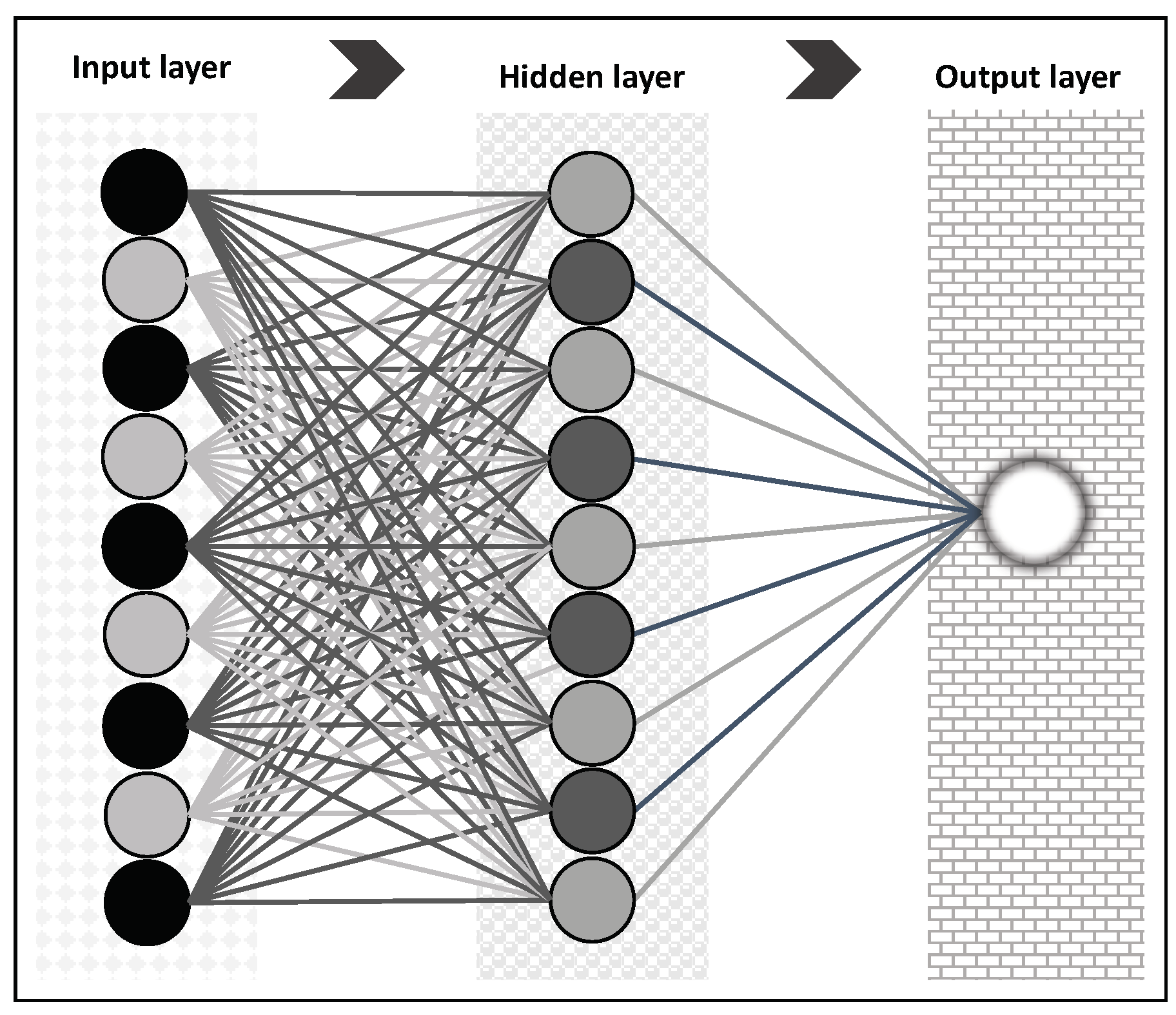
The multilayer perceptron (MLP) model consists of a set of elementary processing elements called neurons [23,40,41,42,43]. These units are organized in architecture with three layers: the input, the hidden, and the output layers. The neurons corresponding to one layer are linked to the neurons of the subsequent layer. Figure 1 illustrates the architecture of this artificial neural network with one hidden layer. The non-linear function $\mathbf{g}(\mathbf{x},\mathbf{w})$ represents the output of the model, where $\mathbf{x}$ is the input signal and $\mathbf{w}$ is its parameter vector. For a three-layer ANN (one hidden layer), the kth output computation is given by the following equation:

$$g_k(\mathbf{x},\mathbf{w})=f_2\left(\sum _{j=1}^{\lambda }{w}_{kj}^{\left[2\right]}{f}_1\left(\sum _{i=1}^d{w}_{ji}^{\left[1\right]}{x}_i+w_{j0}^{\left[1\right]}\right)+w_{k0}^{\left[2\right]}\right),$$

(1)

where $\lambda$ is the number of hidden neurons. An important factor in the specification of neural network models is the choice of the activation function (one of the most used functions is the sigmoid). These can be non-linear functions as long as they are continuous, bounded, and differentiable. The transfer function of hidden neurons $f_1(·)$ should be nonlinear, while for the output neurons, function $f_2(·)$ could be a linear or a nonlinear function.

The MLP operates as follows. The input layer neurons receive the input signal. These neurons propagate the signal to the first hidden layer and do not conduct any processing. The first hidden layer processes the signal and transfers it to the subsequent layer; the second hidden layer propagates the signal to the third, and so on. When the output layer receives and processes the signal, it generates a response. The MLP learns the mapping between input space $\mathcal{X}$ and output space $\mathcal{Y}$ by adjusting the connection strengths between neurons $\mathbf{w}=\{w_1,...,w_d\}$ called weights. Several techniques have been created to estimate the weights, the most popular being the backpropagation learning algorithm.

2.2.2. Self-Organizing Maps

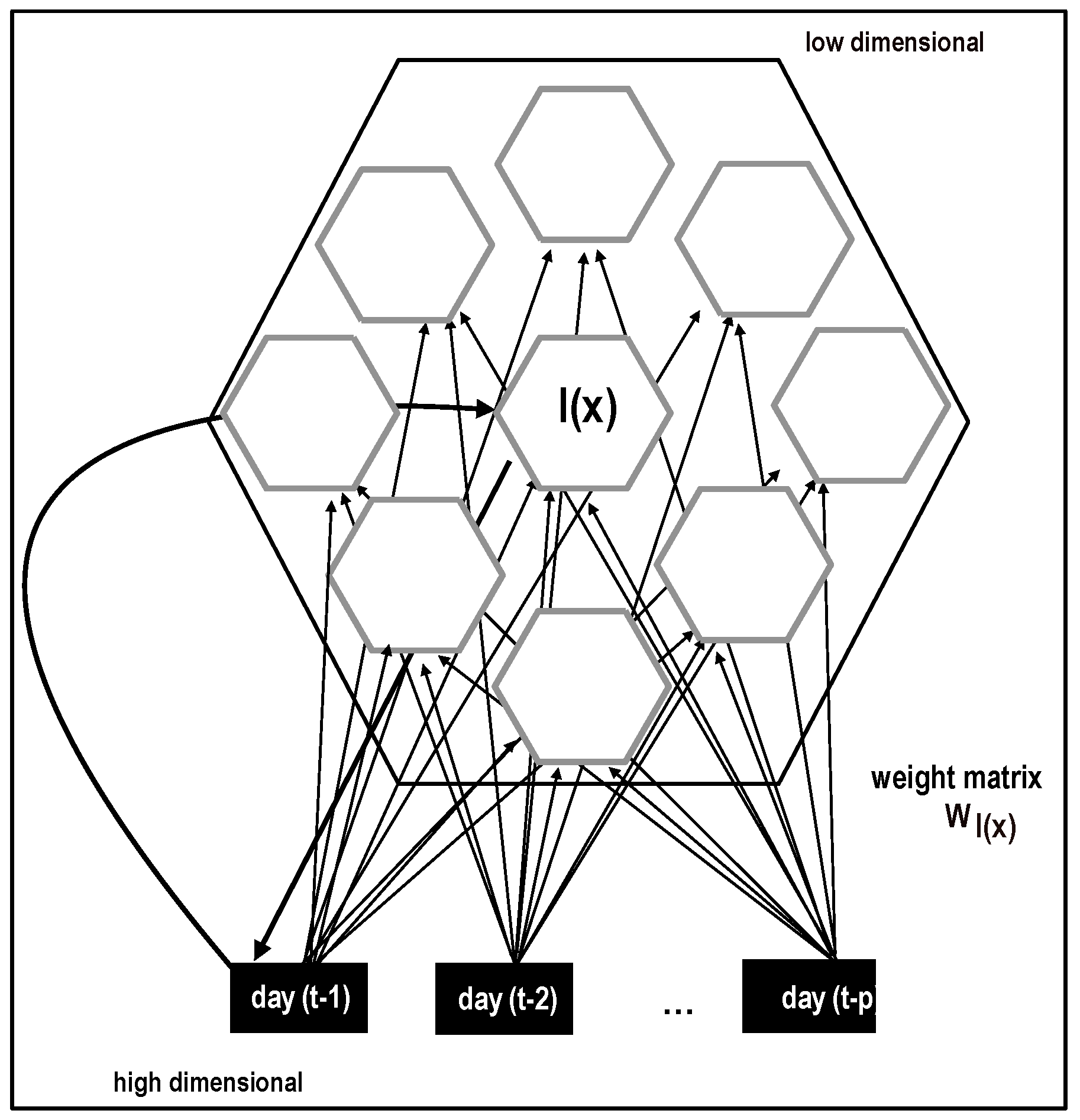
The SOM, introduced by T. Kohonen [35], is an artificial neural network with unsupervised learning. The model projects the topology mapping from the high-dimensional input space into a low-dimensional display (see Figure 2). This model and its variants have been successfully applied in several areas [44].

Map $\mathcal{M}$ consists of an ordered set of M prototypes ${\mathbf{w}}_k\in \mathcal{W}\subseteq {\mathbb{R}}^D$, $k=1\dots M$, with a neighborhood relation between these units forming a grid, where k indexes the location of the prototype in the grid. The most commonly used lattices are the linear, the rectangular, and the hexagonal arrays of cells. In this work, we consider the hexagonal grid where $\kappa \left({\mathbf{w}}_k\right)$ is the vectorial location of the unit ${\mathbf{w}}_k$ in the grid. When the data vector $\mathbf{x}\in {\mathbb{R}}^D$ is presented to model $\mathcal{M}$, it is projected to a neuron position of the low dimensional grid by searching the best matching unit ($bmu$), i.e., the prototype that is closest to the input and is obtained as follows:

$$c\left(\mathbf{x}\right)=arg\underset{{\mathbf{w}}_k\in \mathcal{M}}{min}\left\{d(\mathbf{x},{\mathbf{w}}_k)\right\},$$

(2)

where $d(·,·)$ is some user-defined distance metric (e.g., the Euclidean distance).

This model’s learning process consists of moving the reference vectors toward the current input by adjusting the prototype’s location in the input space. The winning unit and its neighbors adapt to represent the input by applying the following learning rule iteratively:

$${\mathbf{w}}_k(t+1)={\mathbf{w}}_k\left(t\right)+\alpha \left(t\right){\eta }_{c\left({\mathbf{x}}_i\right)}(k,t)[{\mathbf{x}}_i-{\mathbf{w}}_k\left(t\right)]\mathrm{for} \mathrm{all}{\mathbf{w}}_k\in \mathcal{M} \mathrm{and} i=1,...,n,$$

(3)

where the size of the learning step of the units is controlled by both learning rate parameter $0<\alpha \left(t\right)<1$ and neighborhood kernel ${\eta }_{c\left(\mathbf{x}\right)}(k,t)$. Learning rate parameter function $\alpha \left(t\right)$ is a monotonically decreasing function with respect to time. For example, this function could be linear, $\alpha \left(t\right)={\alpha }_0+({\alpha }_f-{\alpha }_0)t/t_{\alpha }$, or exponential, $\alpha \left(t\right)={\alpha }_0{({\alpha }_f/{\alpha }_0)}^{t/t_{\alpha }}$, where ${\alpha }_0$ is the initial learning rate (<1.0), ${\alpha }_f$ is the final rate (≈0.01), and $t_{\alpha }$ is the maximum number of iteration steps to arrive to ${\alpha }_f$. The neighborhood kernel is defined as a decreasing function of the distance between unit ${\mathbf{w}}_k$ and $bmu$ ${\mathbf{w}}_{c\left(\mathbf{x}\right)}$ on the map lattice at time t. A Gaussian function usually produces the kernel.

In practice, the neighborhood kernel is chosen to be wide at the beginning of the learning process to guarantee the global ordering of the map, and both their width and height decrease slowly during learning. Repeated presentations of the training data thus lead to topological order. We can start from an initial state of complete disorder, and the SOM algorithm gradually leads to an organized representation of activation patterns drawn from the input space [45]. In the recent years, there have been some improvements to this model; for example, Salas et al. [46] added flexibility and robustness to the SOM; also, Salas et al. [47] proposed a combination of SOM models.

3. A Self-Organizing Topological Multilayer Perceptron for Extreme Value Forecasting

The proposed model can capture the essential information from the topological structure of the time series, where the best-matching unit of the SOM clusters together similar regimes of the time series. The MLPs as non-linear autoregressive models are expected to improve their combined prediction. Moreover, fewer units learn about the extreme events, and their respective MLPs are specialized in these types of episodes.

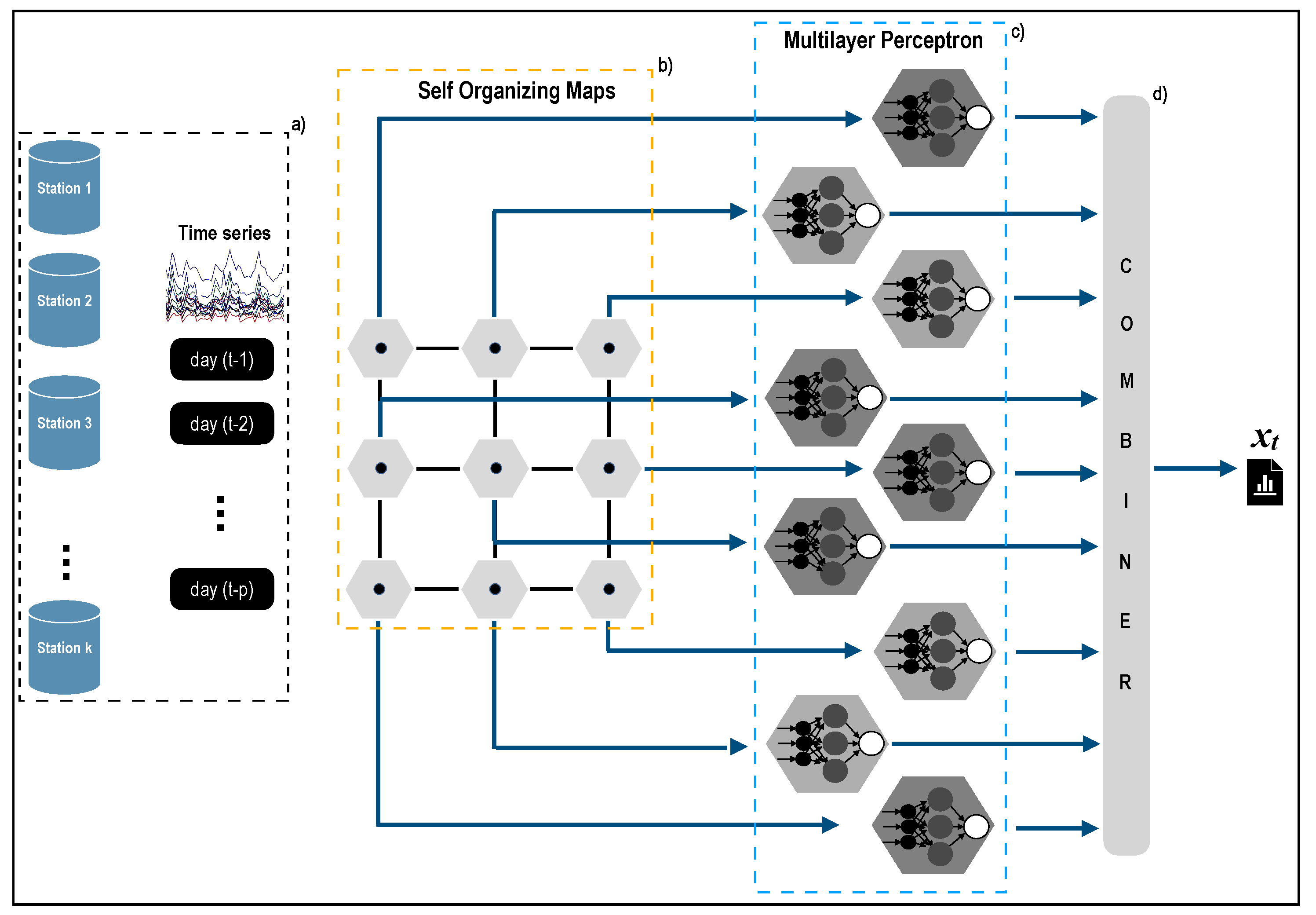
The scheme of the architecture of the SOM-MLP hybrid model is shown in Figure 3. The framework of the SOM-MLP hybrid model consists of four stages. The data are pre-processed and structured in time segments in the first stage. In the second stage, the SOM projects the time segments to their units. The MLP obtains the extreme value forecasting in the third stage. Finally, the outputs are combined with a gating unit to obtain the final response in the fourth stage.

• Stage 1. The monitoring station data are combined into one large data set. Then, we proceed to normalize all the records in the range of $[0,1]$:

  $$X_t=\frac{x_t-min\left\{x_t\right\}}{max\left\{x_t\right\}-min\left\{x_t\right\}}.$$

  (4)
  This article’s data consist of observations collected hourly, for which 24 samples are available daily. The day vector is defined as ${\mathbf{X}}_{t,s}=[X_{t,s}^1,...,X_{t,s}^{24}]$, where $X_{t,s}^l$ is the sample of day t at the lth hour for station s. On one hand, target $y_{t+1,s}$ is built by obtaining a defined percentile of the next day, i.e., $y_{t+1,s}=Percenti{l}_{\gamma }(X_{t+1,s}^1,...,X_{t+1,s}^{24})$. For example, this work considers the 75th and 90th percentiles ($\gamma$ is 75 and 90, respectively). On the other hand, input vector ${\mathbf{X}}_{t,s}$ is constructed as time segments of the selected day-lags. For instance, if we select a lag of p days, i.e., ${\mathbf{X}}_{t,s}=[X_{t,s}^1,...,X_{t,s}^{24}]$, ${\mathbf{X}}_{t-1,s}=[X_{t-1,s}^1,...,X_{t-1,s}^{24}]$ up to ${\mathbf{X}}_{t-p,s}=[X_{t-p,s}^1,...,X_{t-p,s}^{24}]$, then the time segment is built as the concatenation of these day samples as follows:

  $${\mathbb{X}}_{t,s}=[{\mathbf{X}}_{t-p,s},...,{\mathbf{X}}_{t-1,s},{\mathbf{X}}_{t,s}]=[X_{t-p,s}^1,...,X_{t-p,s}^{24},...,X_{t-1,s}^1,...,X_{t-1,s}^{24},X_{t,s}^1,...,X_{t,s}^{24}].$$

  (5)
• Stage 2. This stage aims to recognize topological similarities in the time segments using the SOM network. The SOM model is built with K units corresponding to the optimal number of clusters to group vectors ${\mathbf{X}}_{t,s}$ for each station s. These daily segments are then used to forecast the value for the following day. In this sense, the SOM clusters these segments ${\mathbf{X}}_{t,s}$ with similar contamination patterns for each monitoring station. The nodes are expected to learn contamination patterns; therefore, some of these nodes could have associated high-pollution episodes. The SOM network receives 24 h vectors from each station and associates it with one of the nodes with a similar pollution pattern, which could be low, intermediate, or high-pollution episodes. These episodes can be found on any of the stations. For this reason, SOM is performed for each station independently.
  The SOM model is constructed with K units in a hexagonal lattice. To define the number of units, K, the elbow method, the Calinski–Harabasz index, or the Gap statistic can be used. The Within Cluster Sum of Squares (WCSS) value measures the average squared distance of all the points within a cluster to the cluster centroid. The elbow method graphs the WCSS as a function of the number of clusters, where the bend of the curve offers information on the minimum number of units required by SOM [48,49]. The Calinski–Harabasz index is based on assessing the relationship between variance within clusters and between clusters [50], where the optimal number of clusters maximizes this index [51]. The Gap statistic compares the within-cluster dispersion to its expectation under an appropriate null reference distribution [52].
• Stage 3. The SOM network provides time segments ${\mathbb{X}}_t$ into the best matching unit, $bmu$, i.e., the node with the most similar contamination pattern is associated with the 24-h vector as follows:

  $$c\left({\mathbb{X}}_t\right)=arg\underset{{\mathbf{w}}_k\in \mathcal{M}}{min}\left\{\left|\right|{\mathbb{X}}_t-{\mathbf{w}}_k\left|\right|\right\},$$

  (6)

  where $\left|\right|{\mathbb{X}}_t-{\mathbf{w}}_k\left|\right|$ is the $l^2$-norm.
  For each node of SOM, an MLP is trained to predict the next day’s extreme values $y_{t+1}$ based on inputs ${\mathbb{X}}_t$ associated by the $bmu$. The MLP contains an input layer with D neurons, one hidden layer with $\lambda$ neurons, and an output layer with one neuron. D is the length of time segment input vector ${\mathbb{X}}_t$, and number $\lambda$ is user defined.
• Stage 4. The individual outputs of the MLPs are combined using a combiner operator to generate the final output. We denote the output of the kth MLP as $g^{\left(k\right)}$, $k=1,...,K$, and it corresponds to the kth unit of SOM. In this article, we test the following combining operators that we call the gate:

  (a)

  Best Matching Unit Gate: this gate lets through only the signal from the MLP model corresponding to the best matching unit.

  $$G_{BMU}=\left\{g^{\left(c\right)}|c=arg\underset{{\mathbf{w}}_k\in \mathcal{M}}{min}\left\{d(\mathbf{x},{\mathbf{w}}_k)\right\}\right\}.$$

  (7)

  (b)

  Mean Gate: this gate obtains the average of the MLPs’ outputs:

  $$G_{mean}=\frac{1}{K}\sum _{k=1}^k{g}^{\left(k\right)}.$$

  (8)

  (c)

  Softmax Gate: this gate computes the mean of the softmax of MLPs’ outputs:

  $$G_{softmax}=\frac{1}{K}\sum _{k=1}^{K}softmax\left(g^{\left(1\right)},g^{\left(2\right)},...,g^{\left(K\right)}\right)=\frac{1}{K}\sum _{k=1}^K\frac{exp\left(g^{\left(k\right)}\right)}{{\sum }_{j=1}^{K}exp\left(g^{\left(j\right)}\right)}.$$

  (9)

  (d)

  Maximum Gate: this gate computes the maximum of the outputs of MLPs.

  $$G_{max}=\underset{k\in K}{max}\left\{g^{\left(k\right)}\right\}.$$

  (10)

  (e)

  BMU-MAX Gate (GATE_BM): this gate combines the Best Matching Unit Gate and the Maximum Gate. The gate is controlled by an on–off parameter depending on either the moment of the year or the variability of pollution level.

  $$G_{BM}=\left\{\begin{array}{cc}{G}_{BMU}\hfill & if{V}_x<\theta \hfill \\ Gmax\hfill & \mathrm{otherwise}\hfill \end{array}\right.,$$

  (11)

  where $V_x$ is the variability of the input data, and $\theta$ is a user-defined threshold.

3.1. Data Understanding

Santiago de Chile (SCL) is located at 33.4° S, 70.6° W, with more than six million inhabitants. The metropolitan area of Santiago is one of the most polluted locations in South America, with unfavorable conditions for pollutant dispersion due mainly to the Mediterranean climate and its topography. This condition worsens during the cold season [53], when high concentrations of PM${}_{2.5}$ are observed, mainly due to the fuels used in the industry and transportation, in addition to the prevailing topographic and meteorological conditions [54].

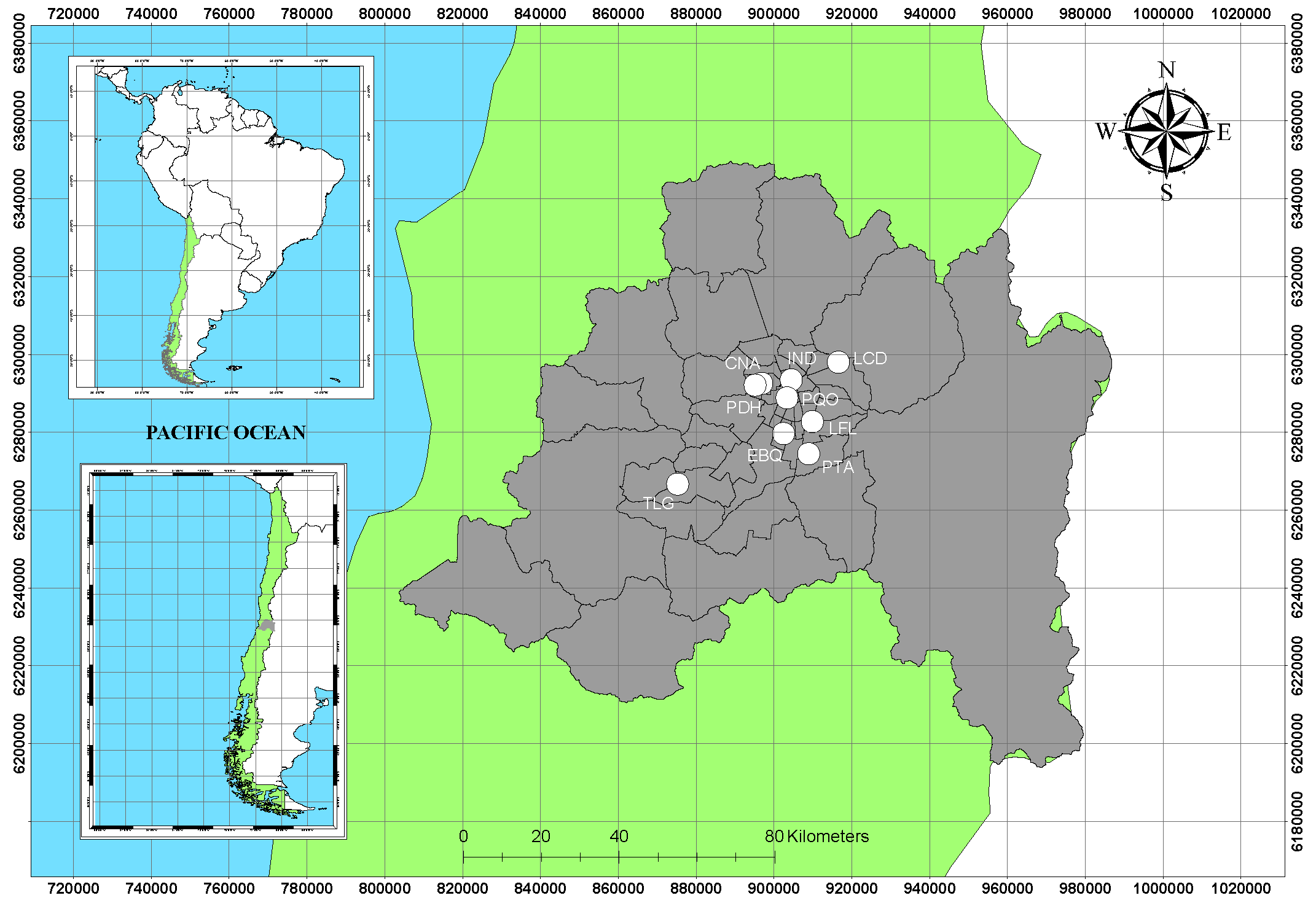
Nine stations belonging to the National Air Quality Information System (SINCA) are located in different locations throughout the metropolitan area of Santiago. These stations constantly monitor pollution contaminants and meteorological conditions of the air. Based on the concentration level of PM${}_{2.5}$ measured by m${}^3$ of air, air quality is classified into five levels as shown in

Table 1. Levels of PM${}_{2.5}$ according to international regulations.

Labels	Levels
1-Good	<50 $\mathsf{\mu }$g/m${}^3$
2-Fair	Between 50 and 80 $\mathsf{\mu }$g/m${}^3$
3-Bad	Between 80 and 110 $\mathsf{\mu }$g/m${}^3$
4-Critical	Between 110 and 170 $\mathsf{\mu }$g/m${}^3$
5-Emergency	>170 $\mathsf{\mu }$g/m${}^3$

. Regulations assert that when the average concentrations during the last 24 hours are classified at Level 3 or higher, restrictions to emissions must be applied immediately. The map of Santiago, Chile shown in Figure 4 contains the locations of the monitoring stations; it was obtained by using the Arcgis 10.4.1 software (https://n9.cl/arcgis-chile), accessed on 21 October 2023, using shapefiles from South America, including the Pacific Ocean, and other countries.

3.2. Performance Metrics

Analysis of the forecasting performance involves calculating the accuracy measures that evaluate the distance between the observed and forecast values. The following indicators were used to evaluate the performance of the proposed method: root mean squared error (RMSE), mean absolute error (MAE), mean squared error (MSE), mean absolute percentage error (MAPE), Spearman correlation index, Pearson coefficient, and coefficient of determination.

• Root of the Mean Squared Error (RMSE):

  $$\mathrm{RMSE}=\sqrt{\frac{1}{n}{\sum }_{i=1}^n{\left(P_i-O_i\right)}^2};$$

  (12)
• Mean Absolute Error (MAE):

  $$\mathrm{MAE}=\frac{1}{n}\sum _{i=1}^n\left|P_i-O_i\right|;$$

  (13)
• Mean Absolute Percentage Error (MAPE):

  $$\mathrm{MAPE}=\frac{1}{n}\sum _{i=1}^n\frac{\left|P_i-O_i\right|}{O_i};$$

  (14)
• Spearman Correlation Index:

  $$S=1-\frac{6{\sum }_{i=1}^n{d}_i^2}{n\left(n^2-1\right)};$$

  (15)
• Pearson coefficient:

  $$\rho =\frac{{\sum }_{i=1}^n\left(P_i-\overline{P}\right)·\left(O_i-\overline{O}\right)}{\sqrt{{\sum }_{i=1}^n{\left(P_i-\overline{P}\right)}^2·{\left(O_i-\overline{O}\right)}^2}};$$

  (16)
• Coefficient of determination:

  $$R^2=1-\left(\frac{{\sum }_{i=1}^n\left({\left(O_i-P_i\right)}^2\right)}{{\sum }_{i=1}^n\left({\left(P_i-\overline{O}\right)}^2\right)}\right);$$

  (17)

  where $O_i$ and $P_i$ are the observed and predicted forecast values, respectively, n is the number of observations, $\overline{P}$ and $\overline{O}$ are the averages for the predicted and observed values, respectively, and $d_i$ is the difference between each pair of values in P and O.

4. Results

4.1. Exploratory Data Analysis

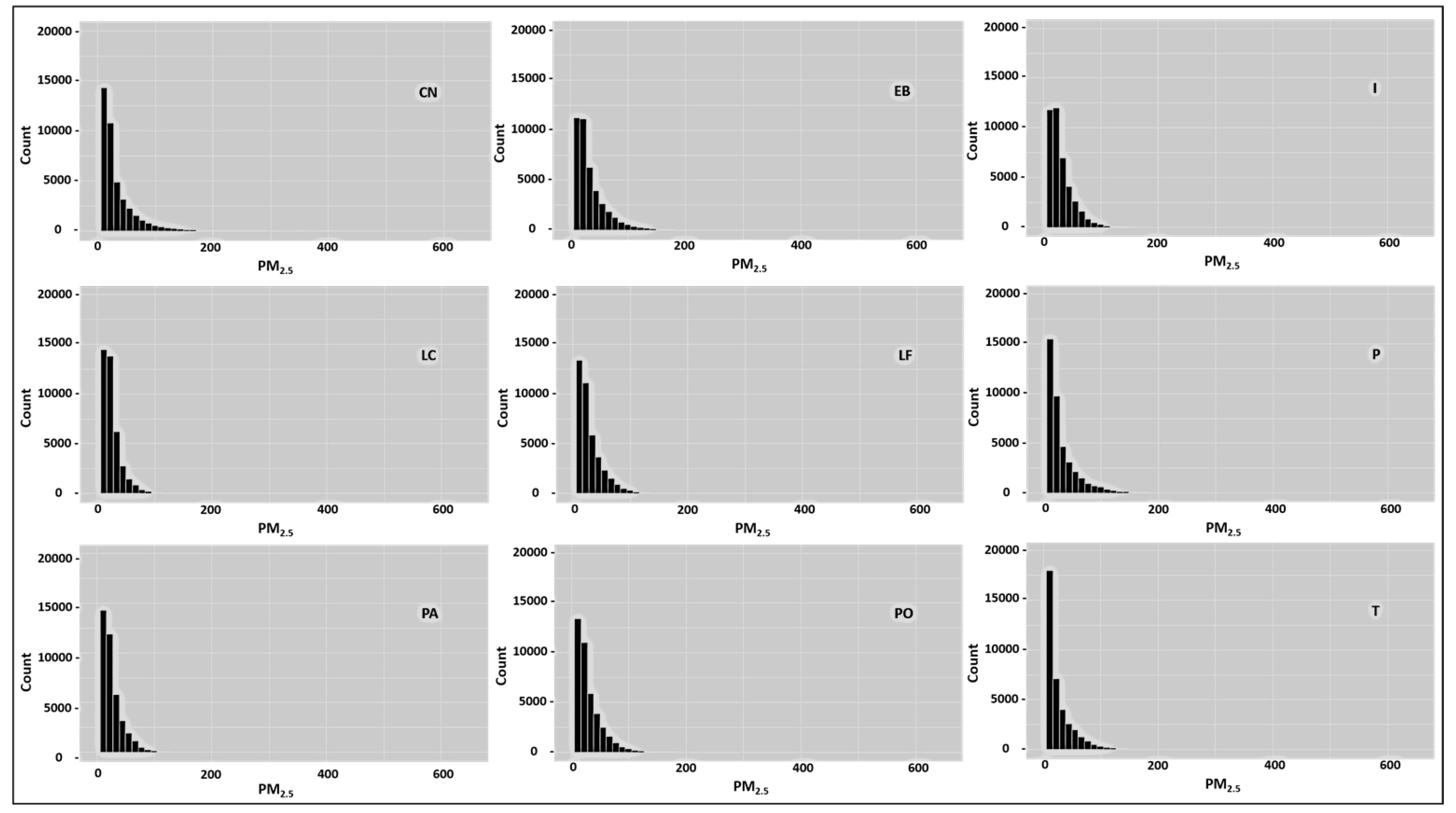
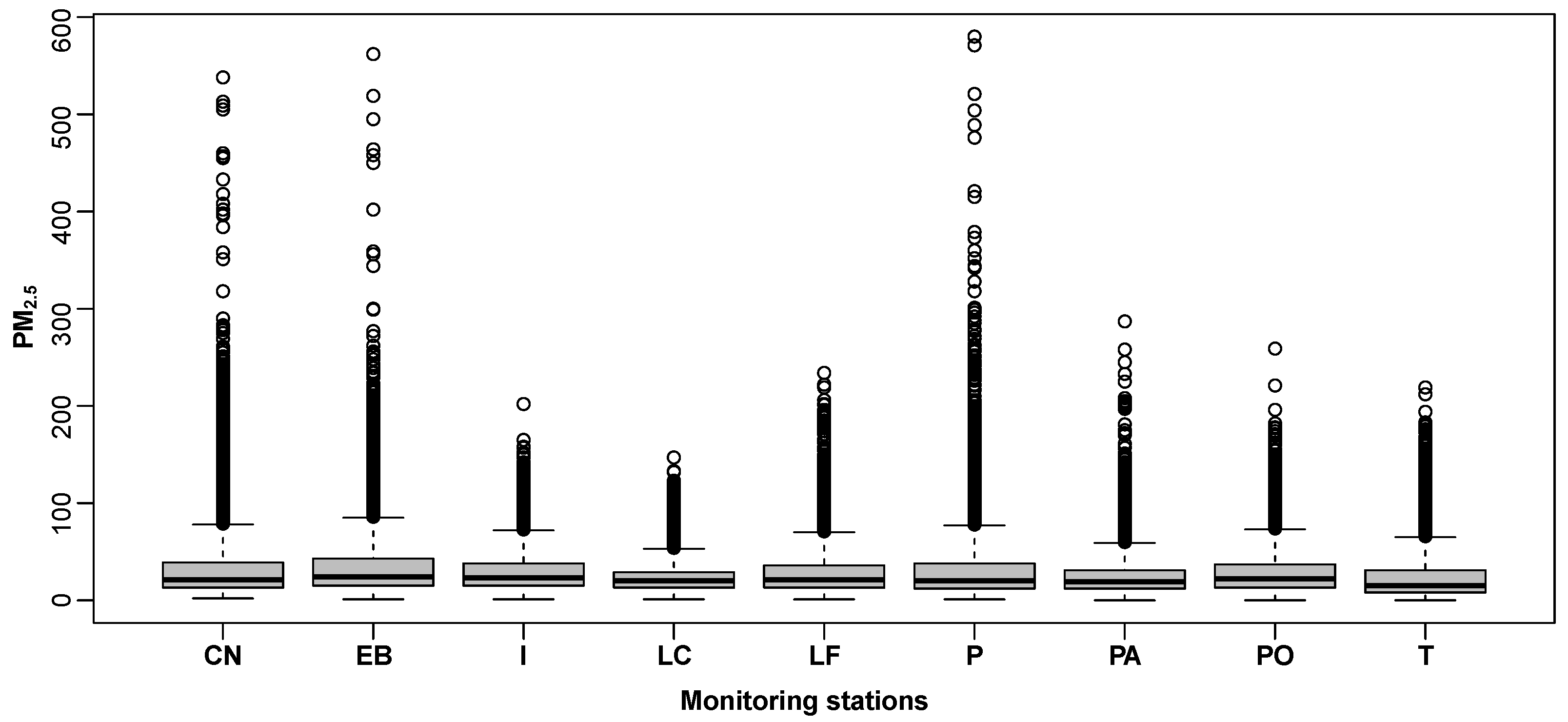
The behavior of the contaminant for each monitoring station is summarized in the histograms and boxplots of Figure 5 and Figure 6, respectively. In general, as can be seen in these figures, they present a probability distribution with a heavy tail, which is evidenced by the appearance of high-contamination episodes. The average PM${}_{2.5}$ in CNA is 31.49 ± 30.22 $\mathsf{\mu }$g/m${}^3$ (

Table 2. Summary statistics of PM${}_{2.5}$ for each monitoring station.

MS	Minimum	1st Q.	Median	Mean ± SD	3rd Q.	Maximum	Variance	Skewness	Kurtosis
CNA	2.00	13.00	21.00	31.49 ± 30.22	39.00	538.00	913.25	3.29	22.39
EBQ	1.00	15.00	24.00	33.25 ± 27.93	43.00	562.00	780.08	2.92	21.22
IND	1.00	15.00	23.00	28.88 ± 19.60	38.00	202.00	384.16	1.48	2.72
LCD	1.00	13.00	20.00	23.42 ± 15.43	29.00	147.00	238.08	1.69	4.03
LFL	1.00	13.00	21.00	27.75 ± 21.33	36.00	234.00	454.97	1.82	5.15
PDH	1.00	12.00	20.00	29.91 ± 29.38	38.00	580.00	863.18	3.52	28.82
PTA	0.00	12.00	19.00	24.51 ± 18.44	31.00	287.00	340.03	2.12	9.60
POH	0.00	13.00	22.00	28.18 ± 21.06	37.00	259.00	443.52	1.65	3.76
TLG	0.00	8.00	15.00	23.68 ± 22.93	31.00	219.00	525.78	2.00	4.96

), which indicates a certain decrease in contamination compared to the results in the study carried out in [55] during the years of 2010–2012.

4.2. Determining the Number of Nodes

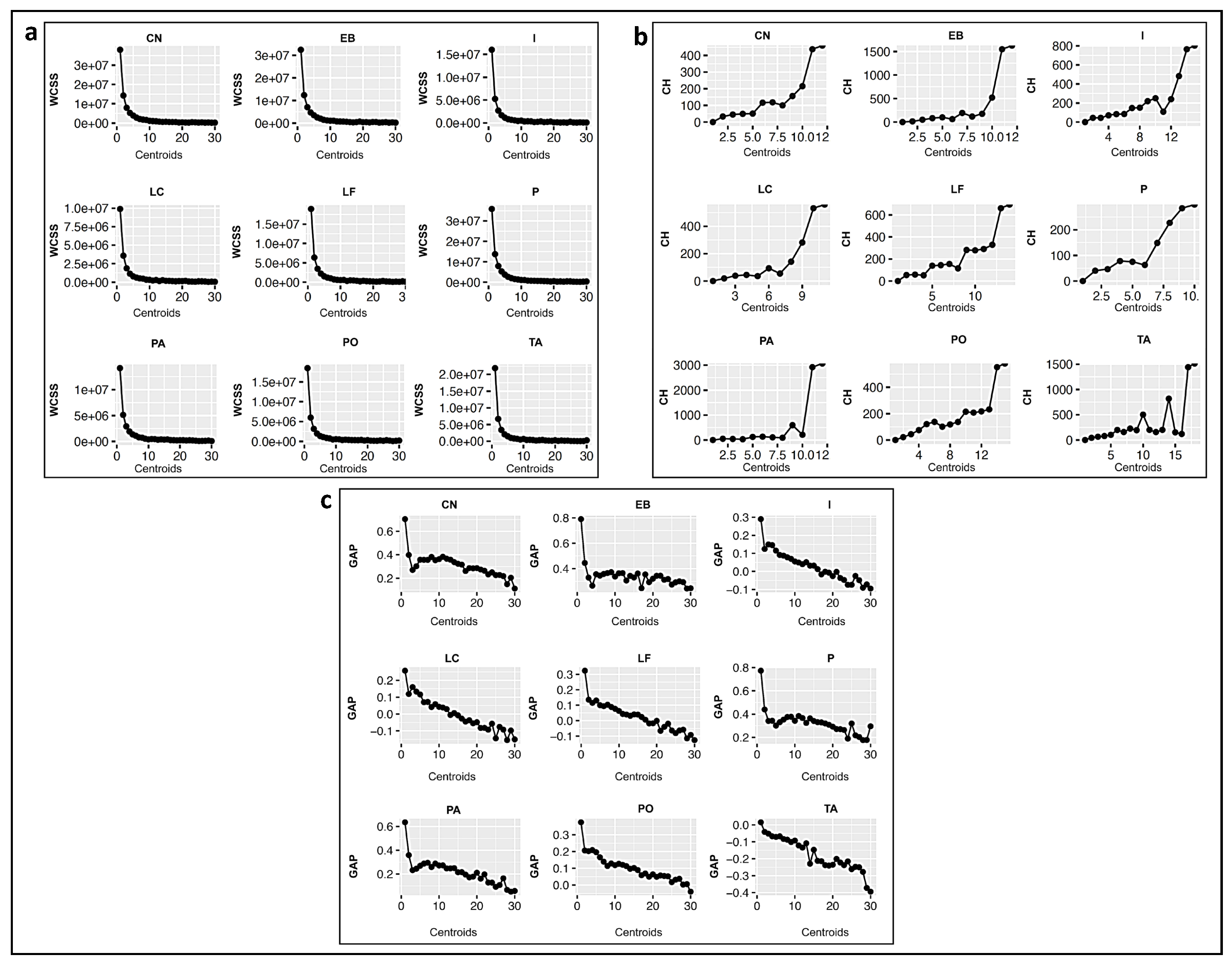
Figure 7 shows the graphs of (a) the Elbow Method, (b) the Calinski–Harabasz index, and (c) the Gap method used to find the optimal number of clusters. First, the Within Cluster Sum of Squares (WCSS) is computed for each cluster for the elbow method. The WCSS is the sum of squares of the distances of each data point in all clusters to their respective centroids. Figure 7a shows that the WCSS measure begins to decrease with a higher number of centroids, where with $K=9$, the WCSS seems to converge. In the application of the Calinski–Harabasz criterion (Figure 7b), we find that in seven of the nine stations, the index obtained begins to grow from $k=9$, showing that after a k greater than 12, the index value seems to stabilize. In this case, we face a scenario in which there is no global maximum, but it can be considered that the optimal value is $K=9$. In Figure 7c, the results of the Gap Statistics method are presented. From the resulting similarities of the nodes analyzed by this criterion, its structure is better defined as a large and single cluster. In many stations, the optimal values for k are between 4 and 12. These methods suggest that $K=9$ is the optimal number of clusters.

5. Performance Results

In this section, an evaluation of the performance of the proposed model SOM-MLP is carried out by comparing it with a global neural network (MLP-Global) and with neural networks obtained for each monitoring station (MLP-Station). The proposed model is applied to predict the next days’ extreme values $y_{t+1}$ given by the percentile 75 and 90 of that day, $Percenti{l}_{\gamma }(X_{t+1}^1,...,X_{t+1}^{24})$. The input vector is time segment ${\mathbb{X}}_t$ constructed with day lags ${\mathbf{X}}_t,{\mathbf{X}}_{t-1}$ and ${\mathbf{X}}_{t-7}$. In this case, 72 neurons are used for the input layer, 96 neurons for the hidden layer, and one neuron for the output layer of the MLP models.

The data used in this study correspond to the concentrations of the PM${}_{2.5}$ pollutant obtained on an hourly scale collected from 1 January 2015 to 30 September 2019. The data are obtained from the SINCA, where a total of nine monitoring stations are considered: Cerro Navia (CNA), Independencia (IND), Las Condes (LCD), Pudahuel (PDH), Parque O’Higgins (POH), La Florida (LFL), El Bosque (EBQ), Puente Alto (PTA) and Talagante (TLG) (see Figure 4).

The data set is divided into training (80%) and test (20%) sets, where the latter has the last 365 days. The training set is used to find the parameters of the neural network models, and the test set is used to evaluate the prediction performance capabilities of the models. The three approaches and the evaluation of the SOM-MLP model performance are implemented through a hold-out validation scheme using 1360 days for training and 365 days for testing.

Table 3. Performance of each model (Mean ± SD): global MLP model, MLP constructed for each station, and the SOM-MLP hybrid model with 4, 9, and 25 neurons.

Metrics	MLP-Global	MLP-Station	SOM-MLP(4)	SOM-MLP(9)	SOM-MLP(25)
MSE	147.860 ± 3.410	127.655 ± 2.609	122.003 ± 9.877	102.293 ± 3.348	101.677 ± 2.792
MAE	7.850 ± 0.121	7.650 ± 0.064	7.266 ± 0.156	6.944 ± 0.069	7.141 ± 0.187
RMSE	12.159 ± 0.141	11.298 ± 0.116	11.037 ± 0.457	10.113 ± 0.164	10.083 ± 0.138
MAPE	24.807 ± 0.247	24.274 ± 0.181	24.050 ± 0.245	22.967 ± 0.176	24.572 ± 1.695

shows the performance of the global MLP method (MLP-Global) and the MLP constructed for each Station (MLP-Station) compared to our proposed hybrid method SOM-MLP with 4, 9 and 25 neurons. The SOM-MLP shows a good compromise between complexity and performance and outperforms the MLP-Global and MLP-Station alternatives.

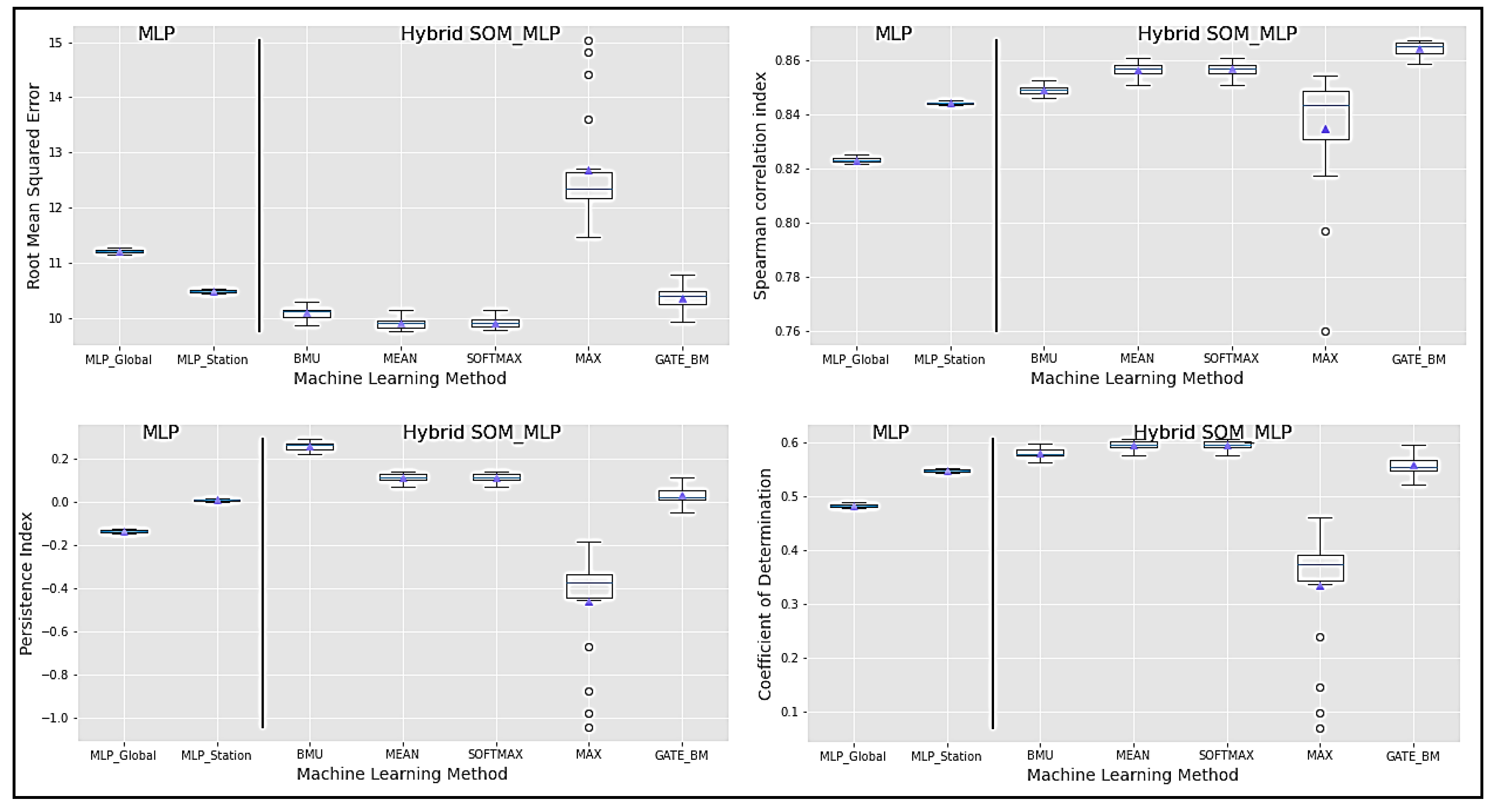
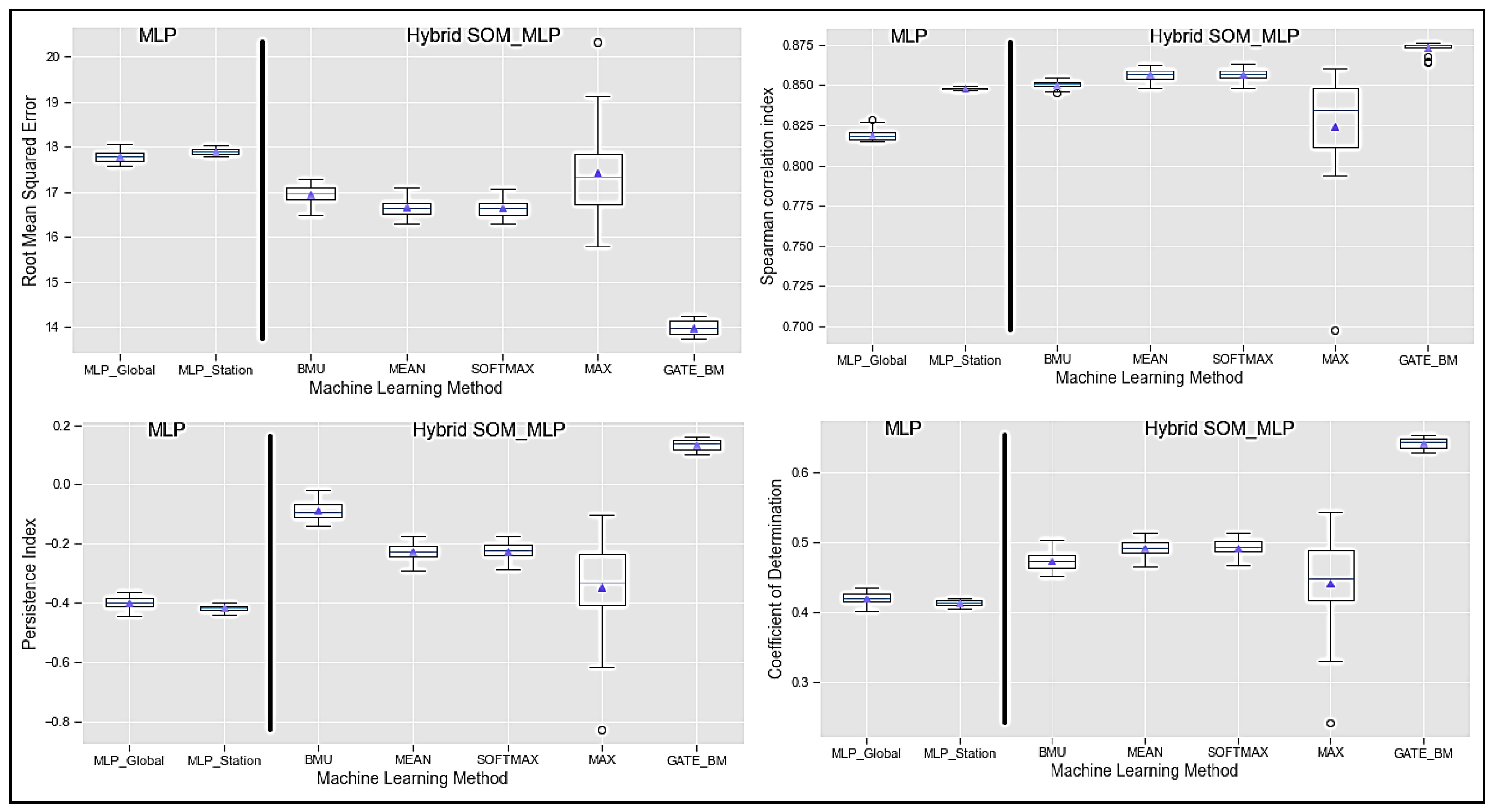
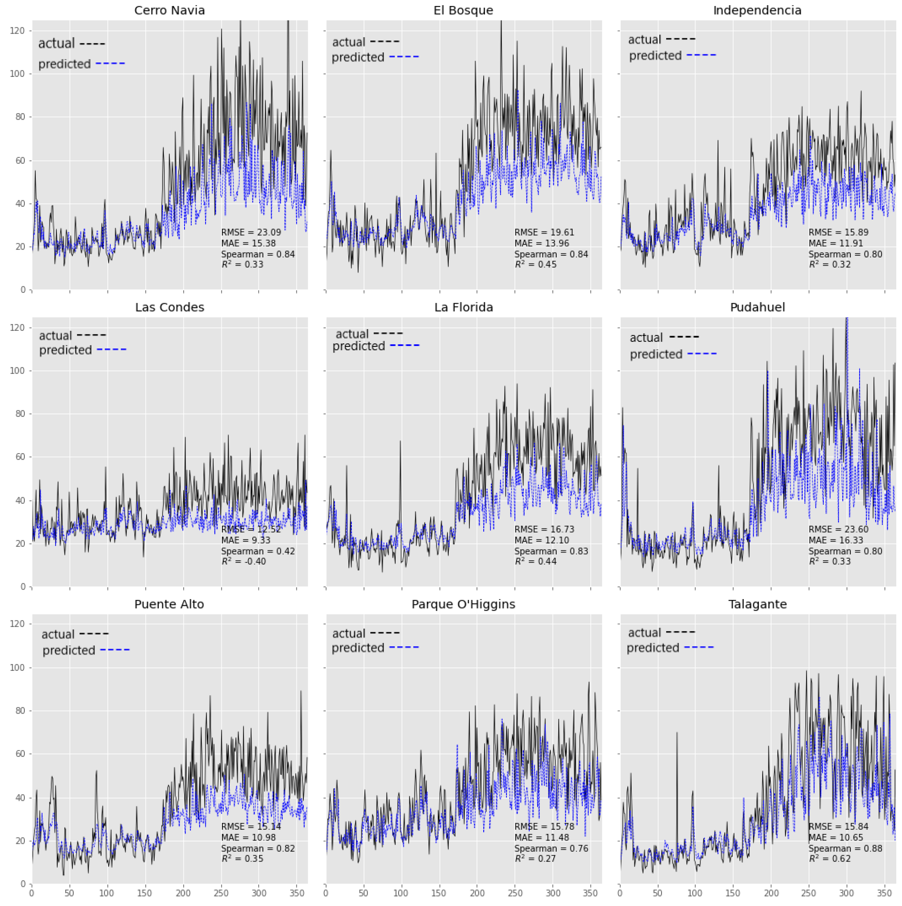
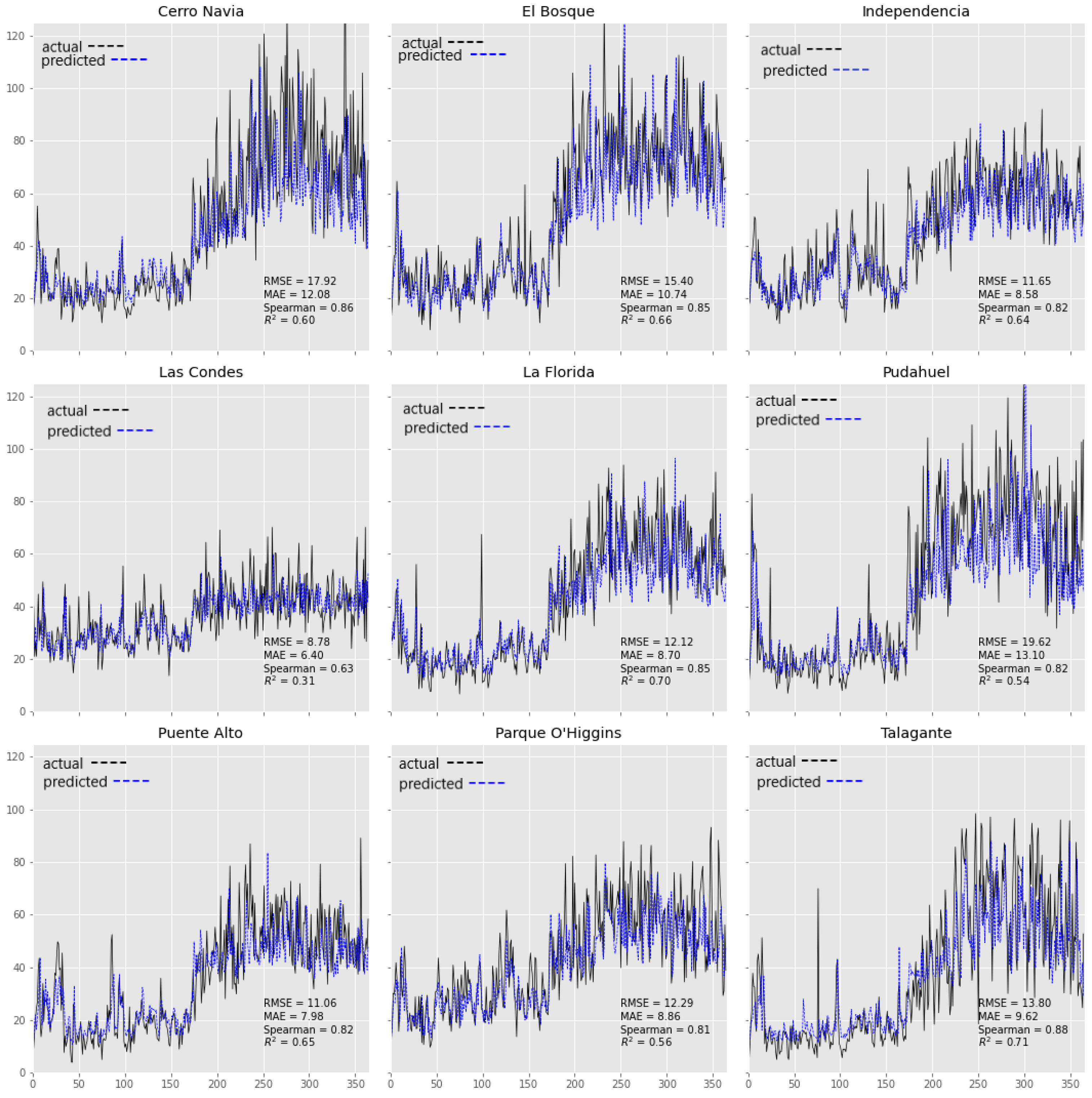
Figure 8 and Figure 9 show the boxplots of the performance metric for each gate for the 75th and 90th percentiles, respectively. Among these are the RMSE, the Spearman correlation index, and the coefficient of determination. For the 90th percentile, it is observed that the GATE_BM is the one with the best performance. It is highlighted that, in extreme values, it is convenient to use the GATE_BM, which does not happen for the 75th percentile since other operators such as BMU, mean, and softmax are suitable in this scenario.

Table 4. Performance metrics obtained with different combiner operators for the 75th percentile. The reported results are the average and standard deviation of 20 runs.

Metrics	BMU	MEAN	SOFTMAX	MAX	GATE_BM
MAE	$6.95\pm 0.060$	$7.33\pm 0.132$	$7.34\pm 0.132$	$10.43\pm 1.065$	$7.10\pm 0.129$
RMSE	$10.10\pm 0.110$	$9.92\pm 0.105$	$9.92\pm 0.104$	$12.68\pm 1.003$	$10.37\pm 0.221$
MAPE	$22.64\pm 0.122$	$28.58\pm 1.051$	$28.64\pm 1.055$	$50.66\pm 7.091$	$24.17\pm 0.452$
Pearson	$0.78\pm 0.005$	$0.78\pm 0.004$	$0.78\pm 0.004$	$0.73\pm 0.025$	$0.80\pm 0.003$
Spearman	$0.85\pm 0.002$	$0.86\pm 0.002$	$0.86\pm 0.002$	$0.84\pm 0.022$	$0.86\pm 0.003$
R${}^2$	$0.58\pm 0.009$	$0.60\pm 0.009$	$0.60\pm 0.009$	$0.33\pm 0.110$	$0.56\pm 0.019$

,

Table 5. Performance metrics obtained with the models for the 75th percentile, for the global MLP model, the MLP constructed for each station, and the SOM-MLP hybrid model. The model with the best performance is the SOM-MLP hybrid model with the GATE_BMU.

Metrics	MLP	MLP Stations	SOM-MLP (BMU)
MAE	$7.75\pm 0.021$	$7.24\pm 0.016$	$6.95\pm 0.060$
RMSE	$11.22\pm 0.035$	$10.48\pm 0.028$	$10.10\pm 0.110$
MAPE	$24.63\pm 0.086$	$23.00\pm 0.042$	$22.64\pm 0.122$
Pearson	$0.73\pm 0.002$	$0.77\pm 0.001$	$0.78\pm 0.005$
Spearman	$0.82\pm 0.001$	$0.84\pm 0.001$	$0.85\pm 0.002$
R${}^2$	$0.48\pm 0.003$	$0.55\pm 0.002$	$0.58\pm 0.009$

,

Table 6. Performance metrics obtained with different combiner operators for the 90th percentile. The reported results are the average and standard deviation of 20 runs.

Metrics	BMU	MEAN	SOFTMAX	MAX	GATE_BM
MAE	$11.60\pm 0.143$	$12.25\pm 0.203$	$12.24\pm 0.204$	$14.31\pm 1.161$	$9.53\pm 0.091$
RMSE	$16.95\pm 0.234$	$16.66\pm 0.205$	$16.65\pm 0.204$	$17.42\pm 1.114$	$13.98\pm 0.159$
MAPE	$25.82\pm 0.198$	$33.56\pm 1.224$	$33.63\pm 1.236$	$54.00\pm 6.651$	$23.64\pm 0.187$
Pearson	$0.77\pm 0.007$	$0.77\pm 0.007$	$0.77\pm 0.007$	$0.70\pm 0.031$	$0.81\pm 0.003$
Spearman	$0.85\pm 0.002$	$0.86\pm 0.004$	$0.86\pm 0.004$	$0.82\pm 0.036$	$0.87\pm 0.004$
R${}^2$	$0.47\pm 0.014$	$0.49\pm 0.013$	$0.49\pm 0.012$	$0.44\pm 0.073$	$0.64\pm 0.008$

and

Table 7. Performance metrics obtained with the models for the 90th percentile, for the global MLP model, MLP constructed for each station, and the SOM-MLP hybrid model. The one that reports the best performance is the SOM-MLP hybrid model with GATE_BM.

Metrics	MLP	MLP Stations	SOM-MLP (GATE_BM)
MAE	$12.23\pm 0.078$	$12.40\pm 0.039$	$9.53\pm 0.091$
RMSE	$17.79\pm 0.127$	$17.90\pm 0.060$	$13.98\pm 0.159$
MAPE	$27.18\pm 0.132$	$26.84\pm 0.060$	$23.64\pm 0.187$
Pearson	$0.72\pm 0.006$	$0.77\pm 0.001$	$0.81\pm 0.003$
Spearman	$0.82\pm 0.004$	$0.85\pm 0.001$	$0.87\pm 0.004$
R${}^2$	$0.42\pm 0.008$	$0.41\pm 0.004$	$0.64\pm 0.008$

report the performances of the models. Furthermore, Figure 10 and Figure 11 show the behavior of the MLP-Station and the hybrid model for each monitoring station, respectively. The highest $R^2$ values of the model fit are observed at the El Bosque, La Florida and Talagante monitoring stations.

6. Discussion

Extreme events in time series refer to episodes with unusually high values that can infrequently, sporadically, or frequently occur [56]. Predicting such extreme events remains a significant challenge [57] due to factors like limited available data, dependence on exogenous variables, or long memory dependence. Qi et al. [57] emphasized the need for neural networks to exhibit adaptive skills in diverse statistical regimes beyond the training dataset.

To address this challenge, we propose a SOM-MLP hybrid model that segments time series into clusters of similar temporal patterns for each station. The MLP acts as a non-linear autoregressive model adapted to these patterns. Our hybrid method demonstrates improved prediction performance, as shown in Table 3, with the SOM-MLP model consisting of nine nodes achieving the best results compared to the MLP-Global and MLP-Station models, exhibiting lower MAE and MAPE metrics.

We utilize aggregating operators for the SOM-MLP model with nine nodes to enhance computational efficiency for both the 75th and 90th percentiles. The best matching unit (BMU) operator performs well for the 75th percentile (see Table 4 and Table 5), while the BMU-MAX gate yields the best results for the 90th percentile (see Table 6 and Table 7). These operators significantly improve the prediction of extreme values, especially during periods of high magnitude and volatility.

The proposed hybrid method, SOM-MLP, effectively captures local similarities in hourly series, enhancing the next day’s 75th or 90th percentile forecasting. While estimating peak values remains challenging, particularly in volatile time series, our approach successfully captures trends and behaviors in each node’s segmented series. This highlights the potential of our proposal for improving extreme value predictions in various time series applications.

7. Conclusions

In this study, we propose a strategy to capture the essential information regarding the topological structure of PM${}_{2.5}$ time series. Our hybrid model demonstrates improved forecasting capabilities, particularly for extreme values. To the best of our knowledge, this is the first paper to employ this approach for predicting extreme air quality time-series events in Santiago, Chile. We observe that recognizing patterns in unique or clustered time series is essential for defining the hybrid model. The comparison of the evaluated models’ performance indicates the potential for improvement through a combined optimization of operators.

Our results demonstrate that the proposed hybrid method outperforms the application of the MLP method per station, which, in turn, exhibits superior performance compared to the Global method. Consequently, these results pave the way for future stages where optimization processes can be implemented within the MLP network structure. Additionally, it is worth exploring the use of alternative neural networks or other methods of interest to enhance the hybrid method further.

This proposal serves as a sophisticated tool for assessing air quality and formulating protective policies for the population. Moreover, the proposed model can be extended to other pollutants, with a specific emphasis on capturing their extreme values and multivariate analysis for seasons, which are often neglected. For instance, in [58], the authors mention their developed model’s inability to predict extreme ozone values. Our proposed model can be applied to analyze this pollutant in future work. Similarly, in [10], a visualization approach for PM${}_{10}$ is proposed, which can be complemented by applying our hybrid method for predictive purposes. Furthermore, this study’s framework can be extrapolated to investigate PM${}_{10}$ in the city of Lima, Peru using neural networks [14].

It is important to highlight that the proposed methodology has some limitations. First, the technique is developed to analyze environmental pollution data based on univariate time series from various sources. Further studies are required for its validation in other contexts (for example, in data related to air quality [59,60,61], solid waste [62], also in academic performance data [63], data related to digital marketing [64] or those based on energy efficiency [65,66]). One of the methodology’s significant limitations is that it does not preserve the time series structure since it assumes an auto-regressive model with a pre-defined lag size.

The proposed approach can also be extended to support the analysis of behaviors in other pollutants in multidimensional cases. Further studies are needed to evaluate the proposed methodology when the time series is decomposed into trend, seasonal, and long-term components, which can be imputed to the model by themselves or together after removing the noise, besides considering incorporating regularization techniques such as Dropout [67] and other strategies to avoid over-parameterization. Moreover, the models can be further improved by introducing geospatial information.

References

1. EPA. Particulate Matter (PM) Basics; Technical Report; United States Environmental Protection Agency: Washington, DC, USA, 2021.
2. Liang, B.; Li, X.L.; Ma, K.; Liang, S.X. Pollution characteristics of metal pollutants in PM2.5 and comparison of risk on human health in heating and non-heating seasons in Baoding, China. Ecotoxicol. Environ. Saf. 2019, 170, 166–171. [Google Scholar] [CrossRef] [PubMed]
3. Gautam, S.; Brema, J. Spatio-temporal variation in the concentration of atmospheric particulate matter: A study in fourth largest urban agglomeration in India. Environ. Technol. Innov. 2020, 17, 100546. [Google Scholar] [CrossRef]
4. Zhou, S.M.; Deng, Q.H.; Liu, W.W. Extreme air pollution events: Modeling and prediction. J. Cent. South Univ. 2012, 19, 1668–1672. [Google Scholar] [CrossRef]
5. Pino-Cortés, E.; Díaz-Robles, L.; Campos, V.; Vallejo, F.; Cubillos, F.; Gómez, J.; Cereceda-Balic, F.; Fu, J.; Carrasco, S.; Figueroa, J. Effect of socioeconomic status on the relationship between short-term exposure to PM2.5 and cardiorespiratory mortality and morbidity in a megacity: The case of Santiago de Chile. Air Qual. Atmos. Health 2020, 13, 509–517. [Google Scholar] [CrossRef]
6. Gautam, S.; Prasad, N.; Patra, A.K.; Prusty, B.K.; Singh, P.; Pipal, A.S.; Saini, R. Characterization of PM2.5 generated from opencast coal mining operations: A case study of Sonepur Bazari Opencast Project of India. Environ. Technol. Innov. 2016, 6, 1–10. [Google Scholar] [CrossRef]
7. Lopez-Restrepo, S.; Yarce, A.; Pinel, N.; Quintero, O.; Segers, A.; Heemink, A. Forecasting PM10 and PM2.5 in the Aburrá Valley (Medellín, Colombia) via EnKF based data assimilation. Atmos. Environ. 2020, 232, 117507. [Google Scholar] [CrossRef]
8. Gualtieri, G.; Carotenuto, F.; Finardi, S.; Tartaglia, M.; Toscano, P.; Gioli, B. Forecasting PM10 hourly concentrations in northern Italy: Insights on models performance and PM10 drivers through self-organizing maps. Atmos. Pollut. Res. 2018, 9, 1204–1213. [Google Scholar] [CrossRef]
9. Liou, N.C.; Luo, C.H.; Mahajan, S.; Chen, L.J. Why is Short-Time PM2.5 Forecast Difficult? The Effects of Sudden Events. IEEE Access 2019, 8, 12662–12674. [Google Scholar] [CrossRef]
10. Encalada-Malca, A.A.; Cochachi-Bustamante, J.D.; Rodrigues, P.C.; Salas, R.; López-Gonzales, J.L. A Spatio-Temporal Visualization Approach of PM10 Concentration Data in Metropolitan Lima. Atmosphere 2021, 12, 609. [Google Scholar] [CrossRef]
11. Solci, C.C.; Reisen, V.A.; Rodrigues, P.C. Robust local bootstrap for weakly stationary time series in the presence of additive outliers. Stoch. Environ. Res. Risk Assess. 2023, 37, 2977–2992. [Google Scholar] [CrossRef]
12. Zhu, S.; Lian, X.; Wei, L.; Che, J.; Shen, X.; Yang, L.; Qiu, X.; Liu, X.; Gao, W.; Ren, X.; et al. PM2.5 forecasting using SVR with PSOGSA algorithm based on CEEMD, GRNN and GCA considering meteorological factors. Atmos. Environ. 2018, 183, 20–32. [Google Scholar] [CrossRef]
13. Feng, X.; Li, Q.; Zhu, Y.; Hou, J.; Jin, L.; Wang, J. Artificial neural networks forecasting of PM2.5 pollution using air mass trajectory based geographic model and wavelet transformation. Atmos. Environ. 2015, 107, 118–128. [Google Scholar] [CrossRef]
14. Cordova, C.H.; Portocarrero, M.N.L.; Salas, R.; Torres, R.; Rodrigues, P.C.; López-Gonzales, J.L. Air quality assessment and pollution forecasting using artificial neural networks in Metropolitan Lima-Peru. Sci. Rep. 2021, 11, 24232. [Google Scholar] [CrossRef]
15. Salas, R.; Bustos, A. Constructing a NARX model for the prediction of the PM10 air pollutant concentration. In Proceedings of the Encuentro Chileno de Computación, Jornada Chilena de Ciencias de la Computación, Valdivia, Chile, 12 November 2005; pp. 7–12. [Google Scholar]
16. Li, S.; Xie, G.; Ren, J.; Guo, L.; Yang, Y.; Xu, X. Urban PM2.5 Concentration Prediction via Attention-Based CNN–LSTM. Appl. Sci. 2020, 10, 1953. [Google Scholar] [CrossRef]
17. Liu, D.R.; Lee, S.J.; Huang, Y.; Chiu, C.J. Air pollution forecasting based on attention-based LSTM neural network and ensemble learning. Expert Syst. 2020, 37, e12511. [Google Scholar] [CrossRef]
18. Russo, A.; Soares, A.O. Hybrid model for urban air pollution forecasting: A stochastic spatio-temporal approach. Math. Geosci. 2014, 46, 75–93. [Google Scholar] [CrossRef]
19. Liu, D.j.; Li, L. Application study of comprehensive forecasting model based on entropy weighting method on trend of PM2.5 concentration in Guangzhou, China. Int. J. Environ. Res. Public Health 2015, 12, 7085–7099. [Google Scholar] [CrossRef]
20. Wang, P.; Zhang, H.; Qin, Z.; Zhang, G. A novel hybrid-Garch model based on ARIMA and SVM for PM2.5 concentrations forecasting. Atmos. Pollut. Res. 2017, 8, 850–860. [Google Scholar] [CrossRef]
21. Paliwal, M.; Kumar, U.A. Neural networks and statistical techniques: A review of applications. Expert Syst. Appl. 2009, 36, 2–17. [Google Scholar] [CrossRef]
22. Kourentzes, N.; Barrow, D.K.; Crone, S.F. Neural network ensemble operators for time series forecasting. Expert Syst. Appl. 2014, 41, 4235–4244. [Google Scholar] [CrossRef]
23. Fu, M.; Wang, W.; Le, Z.; Khorram, M.S. Prediction of particular matter concentrations by developed feed-forward neural network with rolling mechanism and gray model. Neural Comput. Appl. 2015, 26, 1789–1797. [Google Scholar] [CrossRef]
24. Wu, S.; Feng, Q.; Du, Y.; Li, X. Artificial neural network models for daily PM10 air pollution index prediction in the urban area of Wuhan, China. Environ. Eng. Sci. 2011, 28, 357–363. [Google Scholar] [CrossRef]
25. Biancofiore, F.; Busilacchio, M.; Verdecchia, M.; Tomassetti, B.; Aruffo, E.; Bianco, S.; Di Tommaso, S.; Colangeli, C.; Rosatelli, G.; Di Carlo, P. Recursive neural network model for analysis and forecast of PM10 and PM2.5. Atmos. Pollut. Res. 2017, 8, 652–659. [Google Scholar] [CrossRef]
26. Yeganeh, B.; Hewson, M.G.; Clifford, S.; Tavassoli, A.; Knibbs, L.D.; Morawska, L. Estimating the spatiotemporal variation of NO2 concentration using an adaptive neuro-fuzzy inference system. Environ. Model. Softw. 2018, 100, 222–235. [Google Scholar] [CrossRef]
27. Yuan, Q.; Shen, H.; Li, T.; Li, Z.; Li, S.; Jiang, Y.; Xu, H.; Tan, W.; Yang, Q.; Wang, J.; et al. Deep learning in environmental remote sensing: Achievements and challenges. Remote. Sens. Environ. 2020, 241, 111716. [Google Scholar] [CrossRef]
28. Qin, D.; Yu, J.; Zou, G.; Yong, R.; Zhao, Q.; Zhang, B. A novel combined prediction scheme based on CNN and LSTM for urban PM2.5 concentration. IEEE Access 2019, 7, 20050–20059. [Google Scholar] [CrossRef]
29. Sillmann, J.; Thorarinsdottir, T.; Keenlyside, N.; Schaller, N.; Alexander, L.V.; Hegerl, G.; Seneviratne, S.I.; Vautard, R.; Zhang, X.; Zwiers, F.W. Understanding, modeling and predicting weather and climate extremes: Challenges and opportunities. Weather. Clim. Extrem. 2017, 18, 65–74. [Google Scholar] [CrossRef]
30. Miskell, G.; Pattinson, W.; Weissert, L.; Williams, D. Forecasting short-term peak concentrations from a network of air quality instruments measuring PM2.5 using boosted gradient machine models. J. Environ. Manag. 2019, 242, 56–64. [Google Scholar] [CrossRef]
31. Zhang, H.; Wang, Y.; Park, T.W.; Deng, Y. Quantifying the relationship between extreme air pollution events and extreme weather events. Atmos. Res. 2017, 188, 64–79. [Google Scholar] [CrossRef]
32. Bougoudis, I.; Demertzis, K.; Iliadis, L. Fast and low cost prediction of extreme air pollution values with hybrid unsupervised learning. Integr. Comput. Aided Eng. 2016, 23, 115–127. [Google Scholar] [CrossRef]
33. Mijić, Z.; Tasić, M.; Rajšić, S.; Novaković, V. The statistical characters of PM10 in Belgrade area. Atmos. Res. 2009, 92, 420–426. [Google Scholar] [CrossRef]
34. Ercelebi, S.G.; Toros, H. Extreme value analysis of Istanbul air pollution data. Clean-Soil Air Water 2009, 37, 122–131. [Google Scholar] [CrossRef]
35. Kohonen, T. Self-organized formation of topologically correct feature maps. Biol. Cybern. 1982, 43, 59–69. [Google Scholar] [CrossRef]
36. Kohonen, T. The self-organizing map. Proc. IEEE 1990, 78, 1464–1480. [Google Scholar] [CrossRef]
37. Rumelhart, D.E.; Durbin, R.; Golden, R.; Chauvin, Y. Backpropagation: The basic theory. In Backpropagation: Theory, Architectures and Applications; Springer: New York, NY, USA, 1995; pp. 1–34. [Google Scholar]
38. Brockwell, P.; Davis, R.; Davis, R. Introduction to Time Series and Forecasting; Number v. 1-2 in Introduction to Time Series and Forecasting; Springer: Berlin/Heidelberg, Germany, 2002. [Google Scholar]
39. Allende, H.; Moraga, C.; Salas, R. Artificial neural networks in time series forecasting: A comparative analysis. Kybernetika 2002, 38, 685–707. [Google Scholar]
40. Bebis, G.; Georgiopoulos, M. Feed-forward neural networks. IEEE Potentials 1994, 13, 27–31. [Google Scholar] [CrossRef]
41. Hornik, K.; Stinchcombe, M.; White, H. Multilayer feedforward networks are universal approximators. Neural Net. 1989, 2, 359–366. [Google Scholar] [CrossRef]
42. Svozil, D.; Kvasnicka, V.; Pospichal, J. Introduction to multi-layer feed-forward neural networks. Chemom. Intell. Lab. Syst. 1997, 39, 43–62. [Google Scholar] [CrossRef]
43. Elbayoumi, M.; Ramli, N.A.; Yusof, N.F.F.M. Development and comparison of regression models and feedforward backpropagation neural network models to predict seasonal indoor PM2.5–10 and PM2.5 concentrations in naturally ventilated schools. Atmos. Pollut. Res. 2015, 6, 1013–1023. [Google Scholar] [CrossRef]
44. Kohonen, T. Self-Organizing Maps, 3rd ed.; Springer Series in Information Sciences; Springer: Berlin/Heidelberg, Germany, 2001; Volume 30. [Google Scholar]
45. Köküer, M.; Naguib, R.N.; Jančovič, P.; Younghusband, H.B.; Green, R. Chapter 12—Towards Automatic Risk Analysis for Hereditary Non-Polyposis Colorectal Cancer Based on Pedigree Data. In Outcome Prediction in Cancer; Taktak, A.F., Fisher, A.C., Eds.; Elsevier: Amsterdam, The Netherlands, 2007; pp. 319–337. [Google Scholar] [CrossRef]
46. Salas, R.; Moreno, S.; Allende, H.; Moraga, C. A robust and flexible model of hierarchical self-organizing maps for non-stationary environments. Neurocomputing 2007, 70, 2744–2757. [Google Scholar] [CrossRef]
47. Salas, R.; Saavedra, C.; Allende, H.; Moraga, C. Machine fusion to enhance the topology preservation of vector quantization artificial neural networks. Pattern Recognit. Lett. 2011, 32, 962–972. [Google Scholar] [CrossRef]
48. Bholowalia, P.; Kumar, A. EBK-means: A clustering technique based on elbow method and k-means in WSN. Int. J. Comput. Appl. 2014, 105, 17–24. [Google Scholar] [CrossRef]
49. Marutho, D.; Handaka, S.H.; Wijaya, E. The determination of cluster number at k-mean using elbow method and purity evaluation on headline news. In Proceedings of the 2018 International Seminar on Application for Technology of Information and Communication, Semarang, Indonesia, 21–22 September 2018; pp. 533–538. [Google Scholar] [CrossRef]
50. Caliński, T.; Harabasz, J. A dendrite method for cluster analysis. Commun. Stat. Theory Methods 1974, 3, 1–27. [Google Scholar] [CrossRef]
51. Bonaccorso, G. Machine Learning Algorithms; Packt Publishing Ltd.: Birmingham, UK, 2017. [Google Scholar]
52. Tibshirani, R.; Walther, G.; Hastie, T. Estimating the number of clusters in a data set via the gap statistic. J. R. Stat. Soc. Ser. 2001, 63, 411–423. [Google Scholar] [CrossRef]
53. Muñoz, R.C.; Corral, M.J. Surface Indices of Wind, Stability, and Turbulence at a Highly Polluted Urban Site in Santiago, Chile, and their Relationship with Nocturnal Particulate Matter Concentrations. Aerosol Air Qual. Res. 2017, 17, 2780–2790. [Google Scholar] [CrossRef]
54. Perez, P.; Menares, C. Forecasting of hourly PM2.5 in south-west zone in Santiago de Chile. Aerosol Air Qual. Res. 2018, 18, 2666–2679. [Google Scholar] [CrossRef]
55. Perez, P.; Gramsch, E. Forecasting hourly PM2.5 in Santiago de Chile with emphasis on night episodes. Atmos. Environ. 2016, 124, 22–27. [Google Scholar] [CrossRef]
56. Guth, S.; Sapsis, T.P. Machine Learning Predictors of Extreme Events Occurring in Complex Dynamical Systems. Entropy 2019, 21, 925. [Google Scholar] [CrossRef]
57. Qi, D.; Majda, A.J. Using machine learning to predict extreme events in complex systems. Proc. Natl. Acad. Sci. USA 2020, 117, 52–59. [Google Scholar] [CrossRef]
58. Mishra, D.; Goyal, P. Neuro-Fuzzy approach to forecasting Ozone Episodes over the urban area of Delhi, India. Environ. Technol. Innov. 2016, 5, 83–94. [Google Scholar] [CrossRef]
59. da Silva, K.L.S.; López-Gonzales, J.L.; Turpo-Chaparro, J.E.; Tocto-Cano, E.; Rodrigues, P.C. Spatio-temporal visualization and forecasting of PM 10 in the Brazilian state of Minas Gerais. Sci. Rep. 2023, 13, 3269. [Google Scholar] [CrossRef]
60. de la Cruz, A.R.H.; Ayuque, R.F.O.; de la Cruz, R.W.H.; López-Gonzales, J.L.; Gioda, A. Air quality biomonitoring of trace elements in the metropolitan area of Huancayo, Peru using transplanted Tillandsia capillaris as a biomonitor. An. Acad. Bras. Cienc. 2020, 92, 1. [Google Scholar] [CrossRef]
61. Cabello-Torres, R.J.; Estela, M.A.P.; Sánchez-Ccoyllo, O.; Romero-Cabello, E.A.; García Ávila, F.F.; Castañeda-Olivera, C.A.; Valdiviezo-Gonzales, L.; Eulogio, C.E.Q.; De La Cruz, A.R.H.; López-Gonzales, J.L. Statistical modeling approach for PM10 prediction before and during confinement by COVID-19 in South Lima, Perú. Sci. Rep. 2022, 12, 1. [Google Scholar] [CrossRef]
62. Quispe, K.; Martínez, M.; da Costa, K.; Romero Giron, H.; Via y Rada Vittes, J.F.; Mantari Mincami, L.D.; Hadi Mohamed, M.M.; Huamán De La Cruz, A.R.; López-Gonzales, J.L. Solid Waste Management in Peru’s Cities: A Clustering Approach for an Andean District. Appl. Sci. 2023, 13, 1646. [Google Scholar] [CrossRef]
63. Orrego Granados, D.; Ugalde, J.; Salas, R.; Torres, R.; López-Gonzales, J.L. Visual-Predictive Data Analysis Approach for the Academic Performance of Students from a Peruvian University. Appl. Sci. 2022, 12, 11251. [Google Scholar] [CrossRef]
64. Sánchez-Garcés, J.J.; Soria, J.; Turpo-Chaparro, J.E.; Avila-George, H.; López-Gonzales, J.L. Implementing the RECONAC Marketing Strategy for the Interaction and Brand Adoption of Peruvian University Students. Appl. Sci. 2021, 11, 2131. [Google Scholar] [CrossRef]
65. Gonzales, J.; Calili, R.; Souza, R.; Coelho da Silva, F. Simulation of the energy efficiency auction prices in Brazil. Renew. Energy Power Qual. J. 2016, 1, 574–579. [Google Scholar] [CrossRef]
66. López-Gonzales, J.L.; Castro Souza, R.; Leite Coelho da Silva, F.; Carbo-Bustinza, N.; Ibacache-Pulgar, G.; Calili, R.F. Simulation of the Energy Efficiency Auction Prices via the Markov Chain Monte Carlo Method. Energies 2020, 13, 4544. [Google Scholar] [CrossRef]
67. Srivastava, N.; Hinton, G.; Krizhevsky, A.; Sutskever, I.; Salakhutdinov, R. Dropout: A simple way to prevent neural networks from overfitting. J. Mach. Learn. Res. 2014, 15, 1929–1958. [Google Scholar]
Figure 1. Schematic of the architecture of the MLP. The figure shows three layers of neurons: input, hidden and output layers.
Stats 06 00077 g001
Figure 2. Scheme of the architecture of self-organizing maps. This model consists of a single layer of neurons in a discrete lattice called a map. The SOM projects the high-dimensional data into a discrete low-dimensional map.
Stats 06 00077 g002
Figure 3. Proposed self-organized topological multilayer percepton. In the first stage (a), time series are collected from the monitoring stations. In the second stage (b), the self-organizing maps find similar topologies in each monitoring station (complemented by other clustering methods, such as elbow, Calinski–Harabasz, and gap). In the third stage (c), the SOM projects the time segments, and this generates the formation of clusters. An MLP is trained to predict each unit’s extreme values for the next day. In the fourth stage (d), a combiner of the best results of the previous stage is evaluated.
Stats 06 00077 g003
Figure 4. Map with the Metropolitan area of Santiago, Chile (SCL), together with the location of the nine pollutant and weather monitoring stations that belong to SINCA.
Stats 06 00077 g004
Figure 5. Histograms of PM 2.5 for each monitoring station.
Stats 06 00077 g005
Figure 6. Boxplot of PM 2.5 for each monitoring station.
Stats 06 00077 g006
Figure 7. (a) Elbow method, (b) Calinski-Harabasz index and (c) Gap method to determine the optimal number of clusters. It is observed that the three methods converge in determining that the optimal number of centroids is nine.
Stats 06 00077 g007
Figure 8. Performance of the models to forecast the 75th percentile. The SOFTMAX gate shows the best performance.
Stats 06 00077 g008
Figure 9. Performance of the models to forecast the 90th percentile. The BMU-MAX gate shows the best performance.
Stats 06 00077 g009
Figure 10. Forecasting results obtained by the MLP-Station for each station.
Stats 06 00077 g010
Figure 11. Forecasting results obtained by the SOM-MLP with the BMU-MAX gate for each monitoring station.
Stats 06 00077 g011