
Modeling Realized Variance with Realized Quarticity

Abstract
:1. Introduction
2. Related Literature
3. Realized Variance Model
3.1. Model Specification
3.2. Variable Transformations
3.3. Maximum Likelihood Estimation
3.4. Model Evaluation by Pseudo Out-of-Sample Forecasting
4. Empirical Application
4.1. Preliminary Analysis
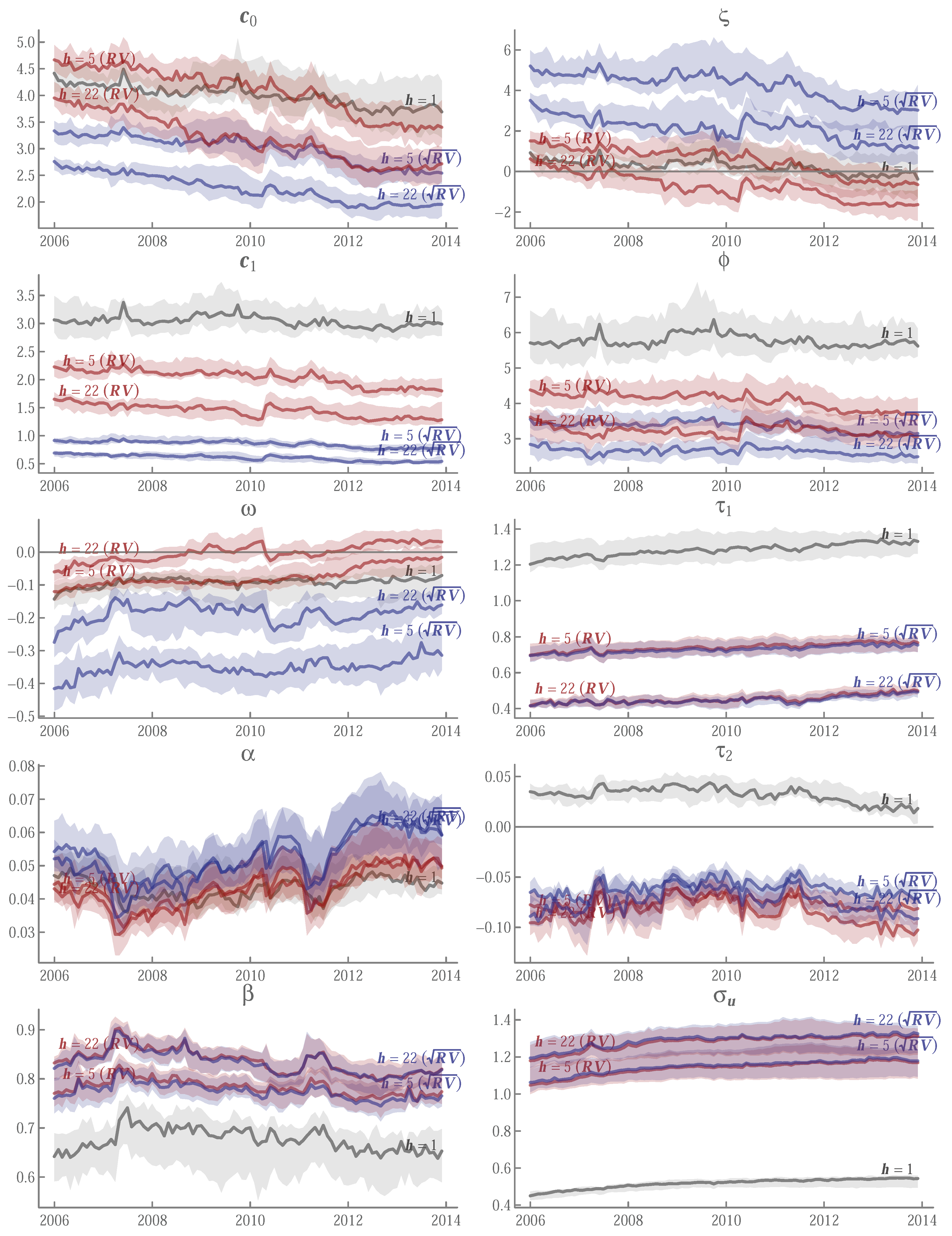
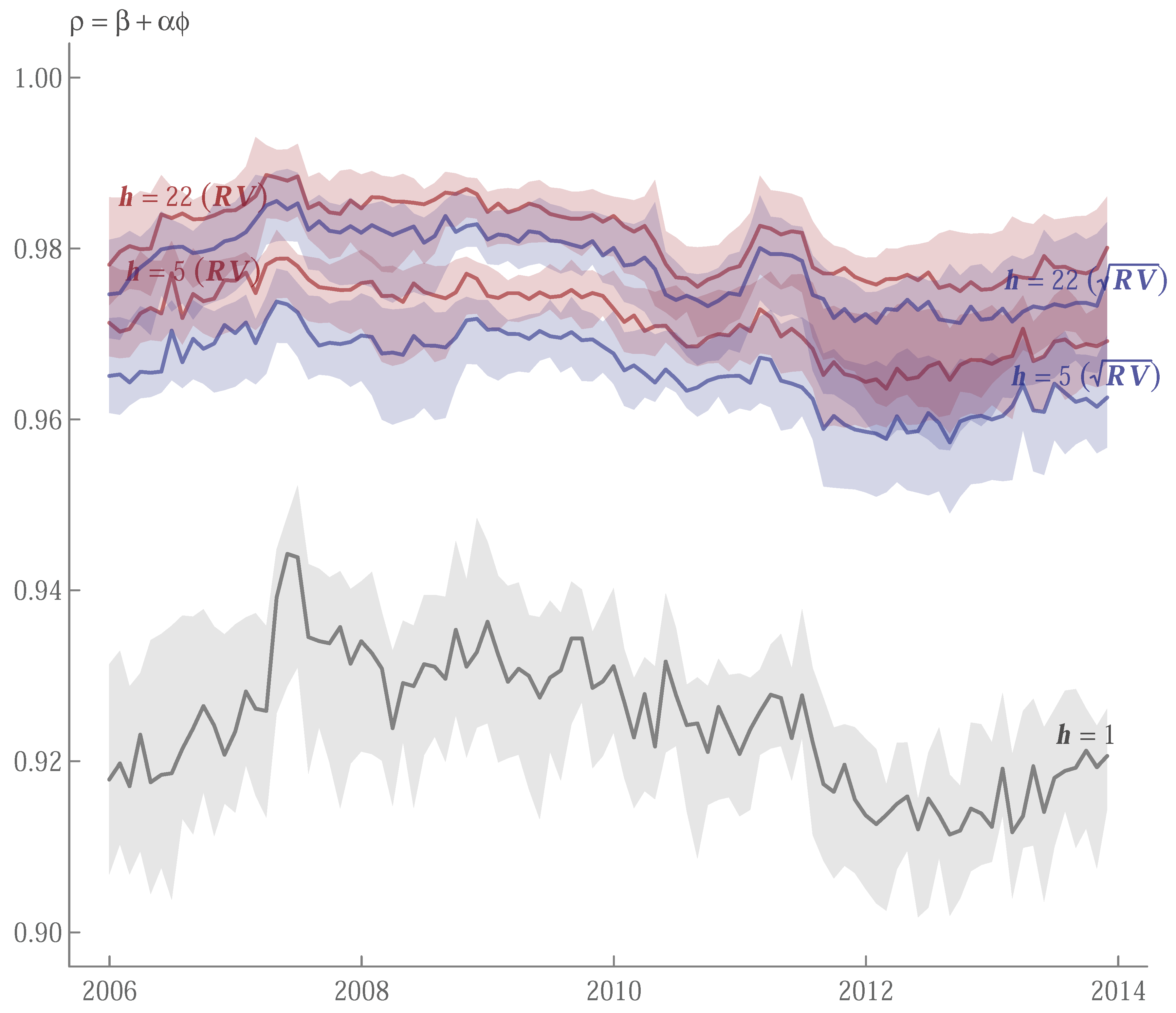
4.2. In-Sample Estimates
4.3. Pseudo Out-of-Sample Forecasts
5. Concluding Remarks
Funding
Conflicts of Interest
Appendix A
Appendix A.1. Summary of Asymptotic Distributions of Realized Variances
Appendix A.2. Derivatives of Log-Likelihood
Appendix A.3. Ticker Symbols

| Symbol | Exchange | Company |
|---|---|---|
| AXP | NYSE | American Express Company |
| BA | NYSE | Boeing Company |
| CAT | NYSE | Caterpillar Inc. |
| CSCO | NASDAQ | Cisco Systems, Inc. |
| CVX | NYSE | Chevron Corporation |
| DD | NYSE | DuPont de Nemours, Inc. |
| DIS | NYSE | Walt Disney Company |
| GE | NYSE | General Electric Company |
| HD | NYSE | Home Depot |
| IBM | NYSE | International Business Machine Corporation |
| INTC | NASDAQ | Intel Corporation |
| JNJ | NYSE | Johnson & Johnson |
| JPM | NYSE | JPMorgan Chase & Co. |
| KO | NYSE | Coca-Cola Company |
| MCD | NYSE | McDonald’s Corporation |
| MMM | NYSE | 3M Company |
| MRK | NYSE | Merck & Co., Inc. |
| MSFT | NASDAQ | Microsoft Corporation |
| NKE | NYSE | Nike, Inc. |
| PFE | NYSE | Pfizer Inc. |
| PG | NYSE | Procter & Gamble Company |
| TRV | NYSE | Travelers Companies, Inc. |
| UNH | NYSE | UnitedHealth Group Incorporated |
| UTX | NYSE | United Technologies Corporation |
| VZ | NYSE | Verizon Communications Inc. |
| WMT | NYSE | Walmart Inc. |
| XOM | NYSE | ExxonMobil Corporation |
| AXP | 11.59 | 262.02 | 2.74 | 17.68 | 0.34 | 2.95 | [0.53] |
| BA | 6.57 | 76.69 | 2.21 | 12.35 | 0.34 | 3.19 | [0.01] |
| CAT | 7.42 | 110.65 | 2.33 | 13.47 | 0.39 | 3.32 | [0.00] |
| CSCO | 4.63 | 36.34 | 1.95 | 8.61 | 0.43 | 2.90 | [0.17] |
| CVX | 15.71 | 400.32 | 3.87 | 35.70 | 0.49 | 4.15 | [0.00] |
| DD | 5.82 | 64.82 | 1.90 | 10.01 | 0.22 | 2.88 | [0.12] |
| DIS | 7.95 | 130.39 | 2.13 | 12.20 | 0.37 | 2.78 | [0.00] |
| GE | 9.79 | 153.91 | 3.26 | 21.52 | 0.53 | 3.52 | [0.00] |
| HD | 7.83 | 121.54 | 2.32 | 13.24 | 0.44 | 3.07 | [0.39] |
| IBM | 6.63 | 78.68 | 2.22 | 11.72 | 0.45 | 2.91 | [0.25] |
| INTC | 4.13 | 31.95 | 1.75 | 7.42 | 0.41 | 2.82 | [0.02] |
| JNJ | 8.23 | 123.38 | 2.25 | 13.72 | 0.27 | 2.82 | [0.02] |
| JPM | 9.63 | 150.45 | 2.99 | 18.91 | 0.44 | 3.20 | [0.01] |
| KO | 6.55 | 83.30 | 2.07 | 11.00 | 0.34 | 2.90 | [0.18] |
| MCD | 12.52 | 283.70 | 2.46 | 18.66 | 0.11 | 2.86 | [0.06] |
| MMM | 13.84 | 348.47 | 2.95 | 23.13 | 0.45 | 3.38 | [0.00] |
| MRK | 21.02 | 774.03 | 3.70 | 36.26 | 0.51 | 3.89 | [0.00] |
| MSFT | 4.69 | 40.03 | 1.82 | 8.40 | 0.37 | 2.82 | [0.02] |
| NKE | 5.28 | 55.88 | 1.82 | 8.77 | 0.35 | 2.71 | [0.00] |
| PFE | 5.39 | 55.00 | 1.97 | 9.89 | 0.38 | 3.01 | [0.91] |
| PG | 9.63 | 171.20 | 2.55 | 16.20 | 0.46 | 3.01 | [0.94] |
| TRV | 15.45 | 401.55 | 3.35 | 26.92 | 0.54 | 3.16 | [0.03] |
| UNH | 8.32 | 126.42 | 2.78 | 16.56 | 0.61 | 3.55 | [0.00] |
| UTX | 7.65 | 106.79 | 2.40 | 13.99 | 0.43 | 3.21 | [0.00] |
| VZ | 7.49 | 114.79 | 2.23 | 12.43 | 0.41 | 3.00 | [0.98] |
| WMT | 8.83 | 176.11 | 1.99 | 11.48 | 0.33 | 2.59 | [0.00] |
| XOM | 13.52 | 322.34 | 3.26 | 26.45 | 0.39 | 3.63 | [0.00] |
| Level | log | |||||||
|---|---|---|---|---|---|---|---|---|
| AXP | 262.02 | −11.84 | −6.52 | −4.04 | 2.95 | 1.23 | 1.12 | −0.39 |
| BA | 76.69 | −4.65 | −3.67 | −3.33 | 3.19 | 0.48 | −0.69 | −0.76 |
| CAT | 110.65 | −6.40 | −2.85 | −2.70 | 3.32 | 0.69 | 0.25 | 0.31 |
| CSCO | 36.34 | −4.15 | −3.54 | −4.33 | 2.90 | 2.65 | 1.71 | 0.61 |
| CVX | 400.32 | −5.57 | −1.81 | −2.12 | 4.15 | 1.76 | 0.91 | 0.96 |
| DD | 64.82 | −5.78 | −3.01 | −3.54 | 2.88 | 0.97 | 0.26 | −0.02 |
| DIS | 130.39 | −3.90 | −5.44 | −4.60 | 2.78 | −0.08 | −0.33 | −0.74 |
| GE | 153.91 | −5.61 | −4.79 | −2.42 | 3.52 | 2.29 | 0.77 | −0.27 |
| HD | 121.54 | −6.96 | −6.33 | −4.83 | 3.07 | 0.05 | −0.22 | −0.34 |
| IBM | 78.68 | −2.68 | −5.52 | −5.31 | 2.91 | 3.42 | 0.68 | 0.58 |
| INTC | 31.95 | −8.25 | −3.40 | −3.97 | 2.82 | 1.73 | 0.91 | 1.08 |
| JNJ | 123.38 | −4.02 | −5.29 | −4.05 | 2.82 | 2.34 | 0.54 | 0.37 |
| JPM | 150.45 | −5.92 | −7.57 | −5.83 | 3.20 | 2.47 | 1.26 | 0.11 |
| KO | 83.30 | −9.07 | −6.21 | −1.32 | 2.90 | 0.16 | 0.45 | 0.24 |
| MCD | 283.70 | −3.78 | −3.10 | −3.35 | 2.86 | −2.05 | −1.78 | −2.16 |
| MMM | 348.47 | −9.81 | −6.43 | −5.93 | 3.38 | 1.33 | 0.83 | 1.31 |
| MRK | 774.03 | −4.70 | −5.44 | −5.44 | 3.89 | −0.17 | −0.42 | −0.73 |
| MSFT | 40.03 | −4.28 | −5.22 | −2.21 | 2.82 | 2.68 | 1.49 | 0.70 |
| NKE | 55.88 | −5.78 | −4.20 | −4.11 | 2.71 | −0.53 | −0.80 | −0.11 |
| PFE | 55.00 | −6.08 | −5.86 | −5.53 | 3.01 | −2.11 | −1.20 | −1.13 |
| PG | 171.20 | −4.68 | −5.68 | −4.26 | 3.01 | 0.76 | 0.09 | 0.31 |
| TRV | 401.55 | −4.15 | −3.98 | −3.38 | 3.16 | 0.98 | 0.84 | 0.54 |
| UNH | 126.42 | −3.38 | −3.32 | −2.21 | 3.55 | 0.37 | 0.43 | 1.23 |
| UTX | 106.79 | −3.06 | −4.61 | −3.57 | 3.21 | 1.73 | 0.66 | 1.25 |
| VZ | 114.79 | −4.63 | −4.75 | −3.99 | 3.00 | −0.79 | −0.19 | 0.73 |
| WMT | 176.11 | −4.98 | −7.64 | −7.70 | 2.59 | 1.69 | 0.92 | −0.27 |
| XOM | 322.34 | −6.14 | −2.92 | −2.88 | 3.63 | 2.07 | 0.86 | 0.64 |
| AXP | 13 October 2008 | 13 October 2008 | 30 September 2008 |
| CAT | 8 October 2008 | 13 October 2008 | |
| 13 October 2008 | |||
| CVX | 13 October 2008 | 13 October 2008 | 16 July 2008 |
| DD | 25 July 2007 | ||
| GE | 17 September 2008 | 17 September 2008 | 17 September 2008 |
| 22 September 2008 | 22 September 2008 | 19 September 2008 | |
| 22 September 2008 | |||
| INTC | 13 October 2008 | 13 October 2008 | 13 October 2008 |
| JNJ | 7 May 2010 | 7 May 2010 | 13 October 2008 |
| 7 May 2010 | |||
| JPM | 31 December 2013 | 13 October 2008 | 13 October 2008 |
| KO | 22 September 2008 | 22 September 2008 | 22 September 2008 |
| MMM | 13 October 2008 | 13 October 2008 | 7 May 2010 |
| 7 May 2010 | 7 May 2010 | ||
| MRK | 28 January 2008 | 28 January 2008 | 28 January 2008 |
| NKE | 7 May 2010 | 7 May 2010 | 7 May 2010 |
| TRV | 19 September 2008 | 23 April 2007 | 23 April 2007 |
| 22 September 2008 | 19 September 2008 | 19 September 2008 | |
| 22 September 2008 | 22 September 2008 | ||
| 13 October 2008 | 26 September 2008 | ||
| UNH | 22 September 2008 | 22 September 2008 | |
| WMT | 9 October 2008 | 9 October 2008 | 9 October 2008 |
| 13 October 2008 | 13 October 2008 | 13 October 2008 | |
| XOM | 13 October 2008 | 13 October 2008 |
| Ticker | ||||||
|---|---|---|---|---|---|---|
| AXP | [0.000] | |||||
| BA | [0.000] | |||||
| CAT | [0.000] | |||||
| CSCO | [0.000] | |||||
| CVX | [0.035] | |||||
| DD | [0.000] | |||||
| DIS | [0.000] | |||||
| GE | [0.000] | |||||
| HD | [0.000] | |||||
| IBM | [0.000] | |||||
| INTC | [0.000] | |||||
| JNJ | [0.000] | |||||
| JPM | [0.000] | |||||
| KO | [0.000] | |||||
| MCD | [0.000] | |||||
| MMM | [0.000] | |||||
| MRK | [0.000] | |||||
| MSFT | [0.000] | |||||
| NKE | [0.000] | |||||
| PFE | [0.000] | |||||
| PG | [0.000] | |||||
| TRV | [0.009] | |||||
| UNH | [0.000] | |||||
| UTX | [0.007] | |||||
| VZ | [0.000] | |||||
| WMT | [0.000] | |||||
| XOM | [0.000] |
Appendix A.4. Forecast Error Diagnostics

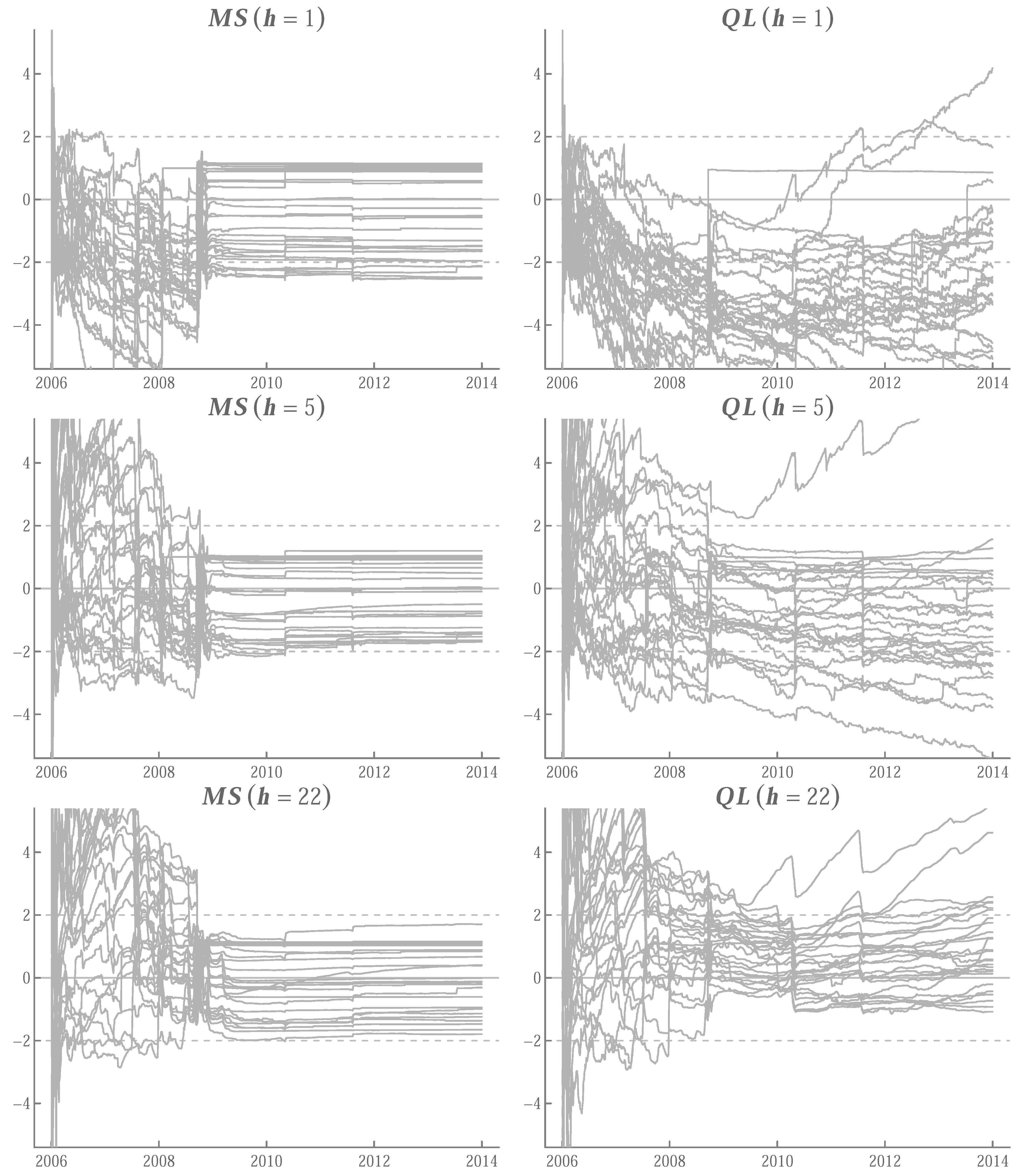
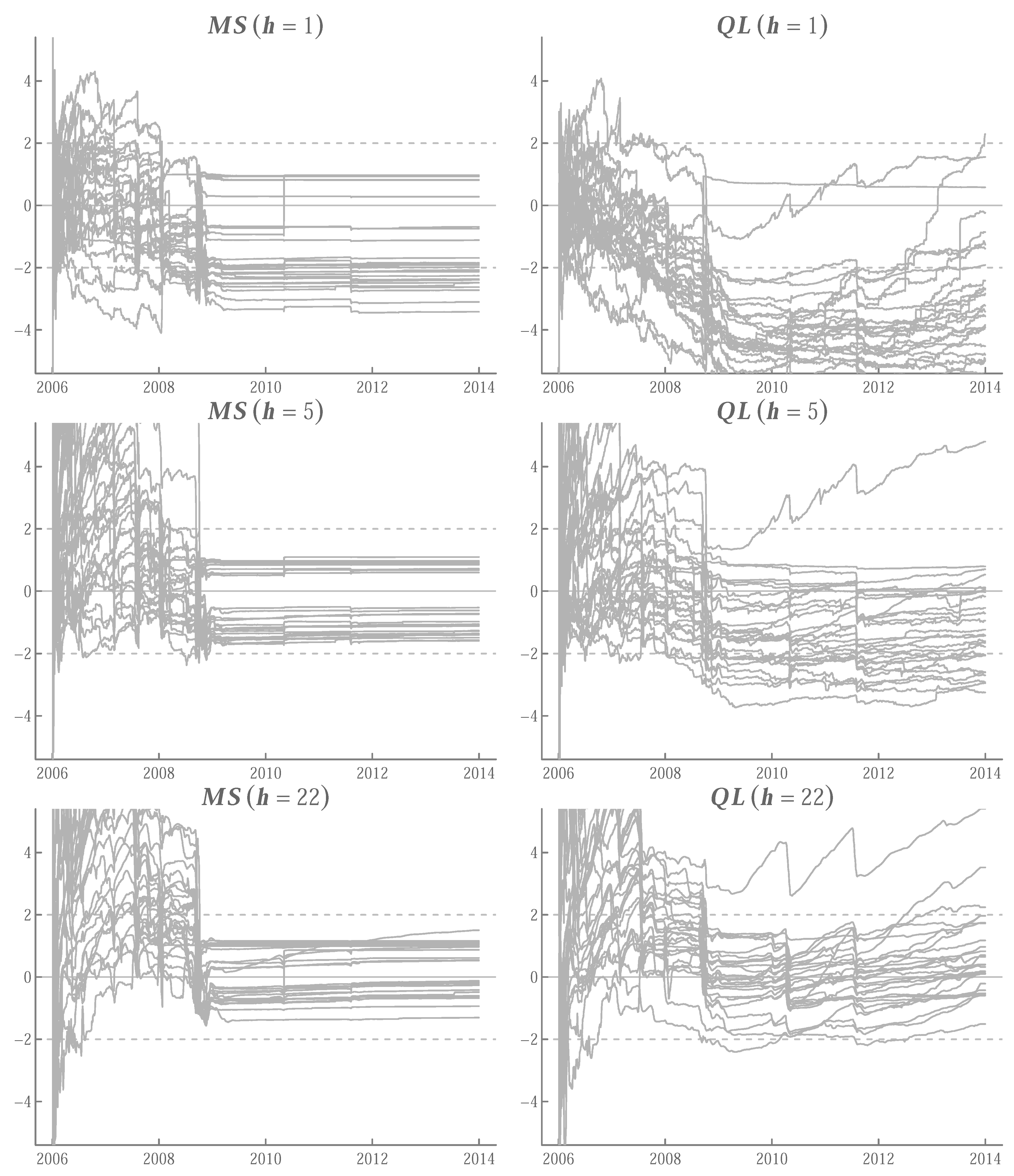
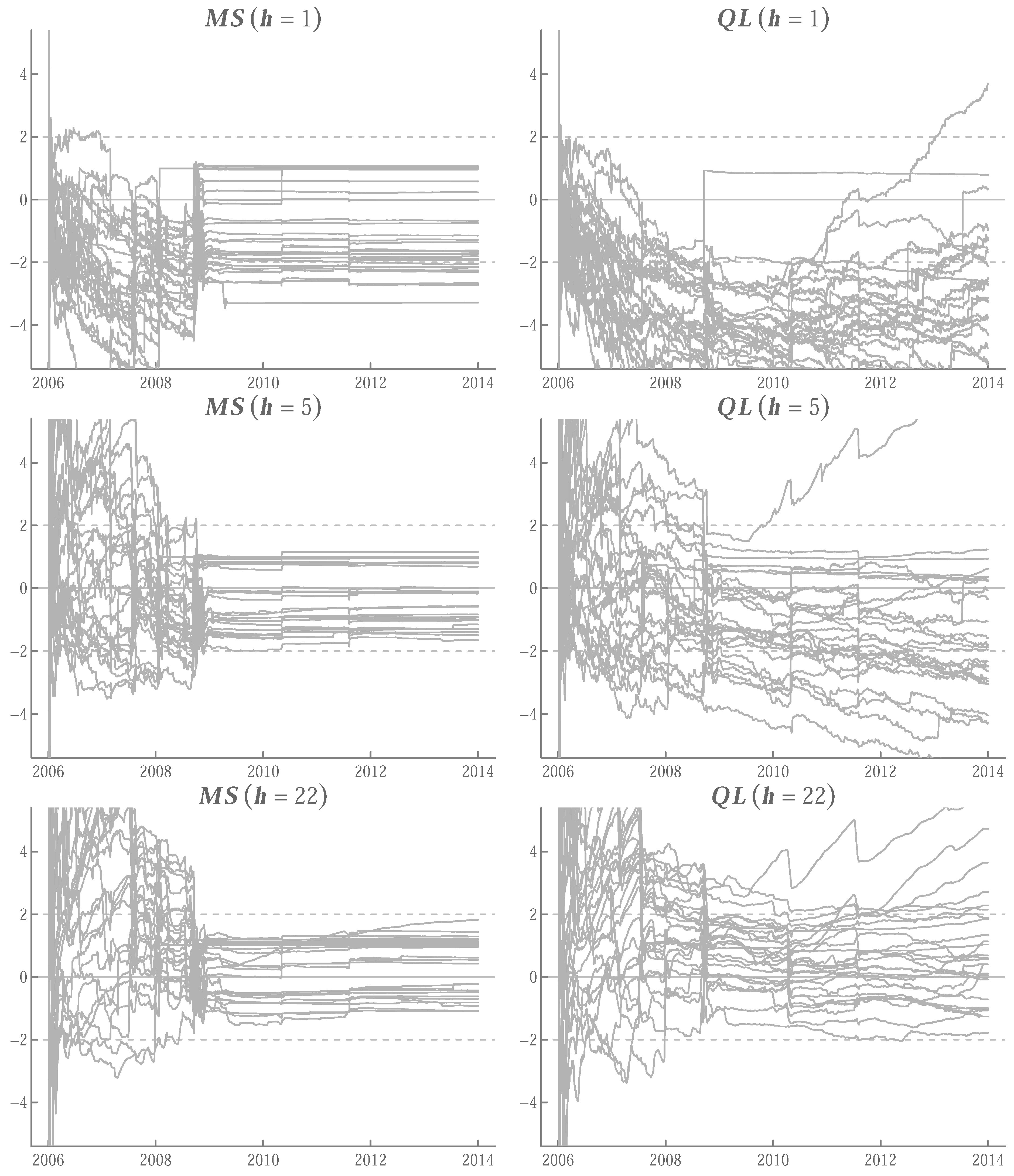
Appendix A.5. Running t-Ratios
References
- Corsi, F. A Simple Approximate Long-Memory Model of Realized Volatility. J. Financ. Econom. 2009, 7, 174–196. [Google Scholar] [CrossRef]
- Rockinger, M.; Jondeau, E. Entropy densities with an application to autoregressive conditional skewness and kurtosis. J. Econom. 2002, 106, 119–142. [Google Scholar] [CrossRef]
- Jondeau, E.; Rockinger, M. Conditional volatility, skewness, and kurtosis: Existence, persistence, and comovements. J. Econ. Dyn. Control 2003, 27, 1699–1737. [Google Scholar] [CrossRef]
- Bali, T.G.; Mo, H.; Tang, Y. The role of autoregressive conditional skewness and kurtosis in the estimation of conditional VaR. J. Bank. Financ. 2008, 32, 269–282. [Google Scholar] [CrossRef]
- Ding, Z.; Granger, C.W.; Engle, R.F. A long memory property of stock market returns and a new model. J. Empir. Financ. 1993, 1, 83–106. [Google Scholar] [CrossRef]
- Comte, F.; Renault, E. Long memory in continuous-time stochastic volatility models. Math. Financ. 1998, 8, 291–323. [Google Scholar] [CrossRef]
- Comte, F.; Coutin, L.; Renault, E. Affine fractional stochastic volatility models. Ann. Financ. 2012, 8, 337–378. [Google Scholar] [CrossRef]
- Gatheral, J.; Jaisson, T.; Rosenbaum, M. Volatility is rough. Quant. Financ. 2018, 18, 933–939. [Google Scholar] [CrossRef]
- Huang, D.; Schlag, C.; Shaliastovich, I.; Thimme, J. Volatility-of-Volatility Risk. J. Financ. Quant. Anal. 2019, 54, 2423–2452. [Google Scholar] [CrossRef]
- Da Fonseca, J.; Zhang, W. Volatility of volatility is (also) rough. J. Futur. Mark. 2019, 39, 600–611. [Google Scholar] [CrossRef]
- Hansen, P.R.; Huang, Z.; Shek, H.H. Realized GARCH: A joint model for returns and realized measures of volatility. J. Appl. Econom. 2012, 27, 877–906. [Google Scholar] [CrossRef]
- Bollerslev, T.; Patton, A.J.; Quaedvlieg, R. Exploiting the errors: A simple approach for improved volatility forecasting. J. Econom. 2016, 192, 1–18. [Google Scholar] [CrossRef]
- Buccheri, G.; Corsi, F. HARK the SHARK: Realized Volatility Modeling with Measurement Errors and Nonlinear Dependencies. J. Financ. Econom. 2021, 19, 614–649. [Google Scholar] [CrossRef]
- Creal, D.; Koopman, S.J.; Lucas, A. Generalized Autoregressive Score Models with Applications. J. Appl. Econom. 2013, 28, 777–795. [Google Scholar] [CrossRef]
- Ding, Y.D. A simple joint model for returns, volatility and volatility of volatility. J. Econom. 2021; in press. [Google Scholar] [CrossRef]
- Ghysels, E.; Santa-Clara, P.; Valkanov, R. There is Risk-Return Trade-off After all. J. Financ. Econ. 2005, 76, 509–548. [Google Scholar] [CrossRef]
- Corsi, F.; Mittnik, S.; Pigorsch, C.; Pigorsch, U. The Volatility of Realized Volatility. Econom. Rev. 2008, 27, 46–78. [Google Scholar] [CrossRef]
- Andersen, T.G.; Bollerslev, T.; Diebold, F.X.; Labys, P. Modeling and Forecasting Realized Volatility. Econometrica 2003, 71, 529–626. [Google Scholar] [CrossRef]
- Geweke, J.; Porter-Hudak, S. The Estimation and Application of Long Memory Time Series Model. J. Time Ser. Anal. 1983, 4, 221–238. [Google Scholar] [CrossRef]
- Hansen, P.R.; Huang, Z. Exponential GARCH Modeling With Realized Measures of Volatility. J. Bus. Econ. Stat. 2016, 34, 269–287. [Google Scholar] [CrossRef]
- Engle, R.F.; Lilien, D.M.; Robins, R.P. Estimating Time Varying Risk Premia in the Term Structure: The ARCH-M Model. Econometrica 1987, 55, 391–407. [Google Scholar] [CrossRef]
- Nelson, D.B. Conditional Heteroskedasticity in Asset Returns: A New Approach. Econometrica 1991, 59, 347–370. [Google Scholar] [CrossRef]
- Barndorff-Nielsen, O.E.; Shephard, N. How Accurate is the Asymptotic Approximation to the Distribution of Realised Variance? In Identification and Inference for Econometric Models; Andrews, D.W.K., Stock, J.H., Eds.; Cambridge University Press: Cambridge, UK, 2005; Chapter 13; pp. 306–331. [Google Scholar]
- Patton, A.J. Volatility forecast comparison using imperfect volatility proxies. J. Econom. 2011, 160, 246–256. [Google Scholar] [CrossRef]
- Duan, N. Smearing Estimate: A Nonparametric Retransformation Method. J. Am. Stat. Assoc. 1983, 78, 605–610. [Google Scholar] [CrossRef]
- Wooldridge, J.M. Introductory Econometrics: A Modern Approach, 7th ed.; Cengage Learning: Boston, MA, USA, 2020. [Google Scholar]
- Diebold, F.X.; Mariano, R.S. Comparing Predictive Accuracy. J. Bus. Econ. Stat. 1995, 13, 253–263. [Google Scholar]
- Barndorff-Nielsen, O.E.; Hansen, P.R.; Lunde, A.; Shephard, N. Designing Realized Kernels to Measure the ex post Variation of Equity Prices in the Presence of Noise. Econometrica 2008, 76, 1481–1536. [Google Scholar]
- Bickel, P.J.; Li, B.; Tsybakov, A.B.; van de Geer, S.A.; Yu, B.; Valdés, T.; Rivero, C.; Fan, J.; van der Vaart, A. Regularization in statistics. Test 2006, 15, 271–344. [Google Scholar] [CrossRef]
- Hastie, T. Ridge Regularization: An Essential Concept in Data Science. Technometrics 2020, 62, 426–433. [Google Scholar] [CrossRef]
- Barndorff-Nielsen, O.E.; Shephard, N. Econometric analysis of realized volatility and its use in estimating stochastic volatility models. J. R. Stat. Soc. Ser. B 2002, 64, 253–280. [Google Scholar] [CrossRef]
- Barndorff-Nielsen, O.E.; Shephard, N. Estimating Quadratic Variation Using Realised Variance. J. Appl. Econom. 2002, 17, 457–477. [Google Scholar] [CrossRef]
- Barndorff-Nielsen, O.E.; Shephard, N. Power and Bipower Variation with Stochastic Volatility and Jumps. J. Financ. Econom. 2004, 2, 1–37. [Google Scholar] [CrossRef]
- Barndorff-Nielsen, O.E.; Shephard, N.; Winkel, M. Limit theorems for multipower variation in the presence of jumps. Stoch. Process. Appl. 2006, 116, 796–806. [Google Scholar] [CrossRef] [Green Version]
- Andersen, T.G.; Bollerslev, T.; Diebold, F.X. Roughing it up: Including jump components in the measurement, modeling and forecasting of return volatility. Rev. Econ. Stat. 2007, 89, 701–720. [Google Scholar] [CrossRef]
| AXP | 1 | 1 | 1 | ||||||
| BA | 0 | 0 | 0 | ||||||
| CAT | 2 | 1 | 0 | ||||||
| CSCO | 0 | 0 | 0 | ||||||
| CVX | 1 | 1 | 1 | ||||||
| DD | 0 | 0 | 1 | ||||||
| DIS | 0 | 0 | 0 | ||||||
| GE | 2 | 2 | 3 | ||||||
| HD | 0 | 0 | 0 | ||||||
| IBM | 0 | 0 | 0 | ||||||
| INTC | 1 | 1 | 1 | ||||||
| JNJ | 1 | 1 | 2 | ||||||
| JPM | 1 | 1 | 1 | ||||||
| KO | 1 | 1 | 1 | ||||||
| MCD | 0 | 0 | 0 | ||||||
| MMM | 2 | 2 | 1 | ||||||
| MRK | 1 | 1 | 1 | ||||||
| MSFT | 0 | 0 | 0 | ||||||
| NKE | 1 | 1 | 1 | ||||||
| PFE | 0 | 0 | 0 | ||||||
| PG | 0 | 0 | 0 | ||||||
| TRV | 2 | 4 | 4 | ||||||
| UNH | 1 | 1 | 0 | ||||||
| UTX | 0 | 0 | 0 | ||||||
| VZ | 0 | 0 | 0 | ||||||
| WMT | 2 | 2 | 2 | ||||||
| XOM | 1 | 1 | 0 | ||||||
| [0.63] | [0.85] | [0.56] | [0.52] | [0.67] | [0.56] | [0.56] | [0.22] | [0.48] | |
| [0.19] | [0.59] | [0.00] | [0.37] | [0.00] | [0.00] | ||||
| [0.37] | [0.15] | [0.48] | [0.33] | [0.44] | [0.78] | ||||
| [0.00] | [0.04] | [0.00] | [0.04] | [0.00] | [0.26] | ||||
Publisher’s Note: MDPI stays neutral with regard to jurisdictional claims in published maps and institutional affiliations. |
© 2022 by the author. Licensee MDPI, Basel, Switzerland. This article is an open access article distributed under the terms and conditions of the Creative Commons Attribution (CC BY) license (https://creativecommons.org/licenses/by/4.0/).
Share and Cite
Kawakatsu, H. Modeling Realized Variance with Realized Quarticity. Stats 2022, 5, 856-880. https://doi.org/10.3390/stats5030050
Kawakatsu H. Modeling Realized Variance with Realized Quarticity. Stats. 2022; 5(3):856-880. https://doi.org/10.3390/stats5030050
Chicago/Turabian StyleKawakatsu, Hiroyuki. 2022. "Modeling Realized Variance with Realized Quarticity" Stats 5, no. 3: 856-880. https://doi.org/10.3390/stats5030050
APA StyleKawakatsu, H. (2022). Modeling Realized Variance with Realized Quarticity. Stats, 5(3), 856-880. https://doi.org/10.3390/stats5030050