Article

Bootstrap Prediction Intervals of Temporal Disaggregation

Department of Mathematics and Statistics, Loyola University Maryland, 4501 N. Charles Street, Baltimore, MD 21210, USA
Stats 2022, 5(1), 190-202; https://doi.org/10.3390/stats5010013
Submission received: 30 December 2021 / Revised: 5 February 2022 / Accepted: 15 February 2022 / Published: 18 February 2022
(This article belongs to the Special Issue Modern Time Series Analysis)

Abstract

:
In this article, we propose an interval estimation method to trace an unknown disaggregate series within certain bandwidths. First, we consider two model-based disaggregation methods called the GLS disaggregation and the ARIMA disaggregation. Then, we develop iterative steps to construct AR-sieve bootstrap prediction intervals for model-based temporal disaggregation. As an illustration, we analyze the quarterly total balances of U.S. international trade in goods and services between the first quarter of 1992 and the fourth quarter of 2020.

1. Introduction

Temporally aggregated data with calendrical periods, e.g., weekly, monthly, quarterly, or annually, have been widely used in various fields because the aggregation technique is simple and convenient for summarizing long sequential measurements and reducing their data lengths. However, it is inevitable that temporal aggregation causes a significant loss of information as a time series of relatively high frequency is compressed into periodic totals of relatively low frequency (see [1,2,3]). Thus, when decompressing the totals, restoring the original information remains a considerable challenge in time series analysis, and numerous solutions for temporal disaggregation have been proposed in modern statistical and econometric literature.
Refs. [4,5,6,7,8] solved disaggregation problems by using additional information obtained from related indicators observed at a desired high frequency. Refs. [9,10] estimated unknown consecutive observations in a disaggregate series based on the model structure of a given aggregate series. In addition, as discussed in [11,12,13], most of recent publications on disaggregation problems focus on exploring point estimation approaches. In other words, there has been, as yet, no systematic examination of interval estimation for temporal disaggregation. The aim of this study is therefore to propose an interval estimation method and to broaden our understanding of temporal disaggregation.
Refs. [14,15,16] introduced an AR-sieve bootstrap procedure to construct nonparametric prediction intervals for linear time series models such as stationary and invertible autoregressive integrated moving-average (ARIMA) processes. AR-sieve bootstrap interval estimation provides a theoretical basis for solving the model-based disaggregation problems of [9,10]. This article is organized as follows. Section 2 presents two model-based disaggregation methods—(1) the generalized least squares (GLS) disaggregation and (2) the ARIMA disaggregation, developed by [9,10], respectively. In Section 3, we propose a modified procedure for finding AR-sieve bootstrap prediction intervals of temporal disaggregation. In Section 4, we analyze a real time series, U.S. international trade balances in goods and services from 1992 to 2020, using the proposed approach. Moreover, some further remarks are given in Section 5.

2. Model-Based Temporal Disaggregation

2.1. The GLS Disaggregation

Suppose that x t is a finite time series for t = 1 , 2 , , n , and the dth differenced series
u t = 1 B d x t = i = 0 d δ i B d i x t
is covariance stationary with mean zero and autocovariance γ u ( j ) for lag j Z , where B is the backshift operator of B j x t = x t j , δ i is the ith coefficient of B + 1 d = i = 0 d δ i B d i , and Z is the set of integers. The m-periodic temporal aggregate (or, simply, m-aggregate) series X T is defined as the nonoverlapping sum of the m sequential observations, x m ( T 1 ) + 1 , x m ( T 1 ) + 2 , , x m T , i.e.,
X T = t = m ( T 1 ) + 1 m T x t = 1 + j = 1 m 1 B j x m T
for T = 1 , 2 , , N and n = m N , and the dth differenced series of X T is given by
V T = 1 B d X T = i = 0 d δ i B d i X t
with autocovariance γ V ( j ) for lag j Z , where B = B m is the backshift operator of B j X T = X T j . Let x = ( x 1 , x 2 , , x n ) , u = ( u d + 1 , u d + 2 , , u n ) , X = ( X 1 , X 2 , , X N ) , and V = ( V d + 1 , V d + 2 , , V N ) . The two expressions (1) and (3) can be rewritten as matrix forms, u = Δ n x and V = Δ N X , where
Δ j = δ 0 δ 1 δ d 0 0 0 δ 0 δ 1 δ d 0 0 0 0 δ 0 δ 1 δ d ( j d ) × j .
In addition, u and V are linearly associated, i.e., V = Ω u with
Ω = w 0 ( N d 1 ) m 0 m w 0 ( N d 2 ) m 0 2 m w 0 ( N d 3 ) m 0 ( N d 1 ) m w ( N d ) × ( n d ) ,
0 k = ( 0 , , 0 ) of size k, and w = ( w 0 , w 1 , , w ( m 1 ) ( d + 1 ) ) , where w i is the ith coefficient of 1 + B + + B m 1 d + 1 = i = 0 ( m 1 ) ( d + 1 ) w i B i and w i = w ( m 1 ) ( d + 1 ) i .
Then, the GLS disaggregation estimates of x and u are given by
x ^ = Δ n 0 d × ( n m d ) | I d 1 m 1 Σ u Ω Σ V 1 Δ N 0 d × ( N d ) | I d X
and
u ^ = Σ u Ω Σ V 1 V ,
respectively, where Σ u and Σ V are the covariance matrices of u t and V T , 0 i × j is the zero matrix of dimension i × j , 1 m = ( 1 , , 1 ) m is the all-ones vector of size m, and I d is the identity matrix of dimension d × d . The symbol ⊗ denotes the Kronecker product, and the vertical and horizontal lines indicate partitioned matrices in (6). (For a more detailed discussion, see [9].) However, the solutions of either (6) or (7) cannot be directly derived unless the covariance matrix Σ u is known. In the following subsection, a model-based solution for the unknown covariance matrix Σ u is discussed.

2.2. Disaggregate ARIMA Models

Ref. [17] showed a linear relationship between the autocovariances of u t and V T such that
γ V ( j ) = 1 + B + + B m 1 2 ( d + 1 ) γ u ( m j + ( m 1 ) ( d + 1 ) )
for j = 0 , 1 , , k and k Z , or equivalently,
Γ V ( k ) = A Γ u ( m k + ( m 1 ) ( d + 1 ) ) ,
where Γ u ( m k + ( m 1 ) ( d + 1 ) ) = ( γ u ( 0 ) , γ u ( 1 ) , , γ u ( m k + ( m 1 ) ( d + 1 ) ) ) , Γ V ( k ) = ( γ V ( 0 ) , γ V ( 1 ) , , γ V ( k ) ) , and A is a resultant coefficient matrix of dimension ( k + 1 ) × ( m k + ( m 1 ) ( d + 1 ) + 1 ) called the aggregation transformation matrix.
Ref. [10] pointed out that (9) is not necessarily a one-to-one mapping, and they solved the disaggregation problem under some reasonable assumptions on ARIMA models. Suppose that an ARIMA ( p , d , q ) model of x t ,
1 i = 1 p ϕ i B i 1 B d x t = 1 j = 1 q θ j B j e t
is a disaggregation solution for an ARIMA ( p , d , r ) model of X T ,
1 i = 1 p Φ i B i 1 B d X T = 1 j = 1 r Θ j B j E T
with r p + d + 1 , where e t and E T are Gaussian white noise with mean zero and constant variances σ e 2 and σ E 2 , respectively. It is also assumed that the AR and MA polynomials of (10), 1 i = 1 p ϕ i B i and 1 j = 1 q θ j B j , share no common factors. The same condition of no common factors is assumed for the model polynomials in (11), 1 i = 1 p Φ i B i and 1 j = 1 r Θ j B j .
Under the condition of no hidden periodicity for aggregation order m (see [18], pp. 512–513), the model parameters ϕ i and θ j in (10) can be solved as follows [10]:
1
The AR part:
  • When m is odd and the AR polynomial of the aggregate model is factorized as
    1 i = 1 p Φ i B i = i = 1 p 1 Ψ i B ,
    the disaggregate AR parameters ϕ i are given by
    1 i = 1 p ϕ i B i = i = 1 p 1 Ψ i 1 / m B .
  • Otherwise, a disaggregate model cannot be uniquely determined.
2
The MA part:
Ref. [19] showed that the m-aggregate model for ARIMA ( p , d , q ) with q p + d + 1 is ARIMA ( p , d , r ) with r p + d + 1 . Thus, it is reasonable to assume that the maximum MA order of the disaggregate model is q = p + d + 1 .
Consider k = p + d + 1 in (9). Because γ V ( j ) for j > d + 1 depends only on γ u ( i ) for i > d + 1 , the aggregation transformation matrix A in (9) can be partitioned as
A = P 11 P 12 0 p × ( d + 2 ) P 22 ,
where P 11 is a square matrix of size d + 2 , such as Γ V ( d + 1 ) = P 11 Γ u ( d + 1 ) , and P 12 and P 22 are block matrices of dimensions ( d + 2 ) × ( ( l + 1 ) ( d + 2 ) ) and p × ( ( l + 1 ) ( d + 2 ) ) , respectively, with l = m ( p + d + 1 ) + ( m 1 ) ( d + 1 ) .
Using the approaches given in Theorem 1 of [10], Equation (9) is rewritten as
Γ V ( p + d + 1 ) = P 11 P 12 H 0 p × ( d + 2 ) P 22 H Γ u ( p + d + 1 ) ,
where H is a coefficient matrix of dimension ( ( l + 1 ) ( d + 2 ) ) × p , relating γ u ( i ) to itself for d + 2 i p + d + 1 and γ u ( i ) to γ u ( d + 2 ) , γ u ( d + 3 ) , , γ u ( p + d + 1 ) for i > p + d + 1 . In other words, if the matrix in (15) is not singular, we have
Γ u ( p + d + 1 ) = P 11 P 12 H 0 p × ( d + 2 ) P 22 H 1 Γ V ( p + d + 1 ) .
As discussed in [10], the inverse matrix in (16) exists under the condition of no hidden periodicity for order m. Then, we can derive the disaggregate MA parameters θ j from the autocovariances γ u ( 0 ) , γ u ( 1 ) , , γ u ( p + d + 1 ) included in Γ u ( p + d + 1 ) .
Two special cases of the ARIMA disaggregation are illustrated below.
Example 1.
Consider an m-aggregate series X T written as the ARIMA ( 1 , 1 , 0 ) model
1 Φ B 1 B X T = E T
with aggregation order m = 3 . We remark that the ARIMA ( 1 , 1 , 3 ) model
1 ϕ B 1 B x t = 1 θ 1 B θ 2 B 2 θ 3 B 3 e t
is a possible solution for the unknown disaggregate series x t , under the conditions of p = 1 and q p + d + 1 = 3 . We find the model parameters of (18) as follows.
  • The disaggregate AR parameter:
    From Equations (12) and (13), it is clear that ϕ = Φ 1 / 3 .
  • The disaggregate MA parameters:
    Let V T = 1 B X T and u t = 1 B x t . From (8) and (9), we find the linear relationship γ V ( j ) = 1 + B + B 2 4 γ u ( 3 j + 4 ) for j = 0 , 1 , 2 , 3 , and so
    Γ V ( 3 ) = P 11 P 12 0 1 × 3 P 22 Γ u ( 13 ) ,
    where
    P 11 = 19 32 20 4 11 16 0 0 1 , P 12 = 8 2 0 0 0 0 0 0 0 0 0 19 16 10 4 1 0 0 0 0 0 0 4 10 16 19 16 10 4 1 0 0 0 ,
    and P 22 = ( 0 , 0 , 1 , 4 , 10 , 16 , 19 , 16 , 10 , 4 , 1 ) . Moreover, since the AR ( 1 ) component implies γ u ( k ) = ϕ γ u ( k 1 ) = Φ 1 / 3 γ u ( k 1 ) for k > 3 , Γ u ( 13 ) can be rewritten as
    Γ u ( 13 ) = I 3 0 3 × 1 0 11 × 3 H Γ u ( 3 ) ,
    where H = ( 1 , Φ 1 / 3 , Φ 2 / 3 , , Φ 10 / 3 ) . We therefore obtain
    Γ V ( 3 ) = 19 32 20 8 + 2 Φ 1 / 3 4 11 16 19 + 16 Φ 1 / 3 + 10 Φ 2 / 3 + 4 Φ + Φ 4 / 3 0 0 1 4 + 10 Φ 1 / 3 + 16 Φ 2 / 3 + 19 Φ + 16 Φ 4 / 3 + 10 Φ 5 / 3 + 4 Φ 2 + Φ 7 / 3 0 0 0 Φ 2 / 3 + 4 Φ + 10 Φ 4 / 3 + 16 Φ 5 / 3 + 19 Φ 2 + 16 Φ 7 / 3 + 10 Φ 8 / 3 + 4 Φ 3 + Φ 10 / 3 Γ u ( 3 ) .
    When the matrix in (21) is not a singular matrix, the autocovariances γ u ( 0 ) , γ u ( 1 ) , γ u ( 2 ) , and γ u ( 3 ) can be solved. Consider w t = 1 Φ 1 / 3 B u t , which is MA ( 3 ) from (18). The autocovariances of w t are expressed as
    γ w ( 0 ) = 1 + Φ 2 / 3 γ u ( 0 ) 2 Φ 1 / 3 γ u ( 1 ) = 1 + θ 1 2 + θ 2 2 + θ 3 2 σ e 2 , γ w ( 1 ) = Φ 1 / 3 γ u ( 0 ) + 1 + Φ 2 / 3 γ u ( 1 ) Φ 1 / 3 γ u ( 2 ) = θ 1 + θ 1 θ 2 + θ 2 θ 3 σ e 2 , γ w ( 2 ) = Φ 1 / 3 γ u ( 1 ) + 1 + Φ 2 / 3 γ u ( 2 ) Φ 1 / 3 γ u ( 3 ) = θ 2 + θ 1 θ 3 σ e 2 , γ w ( 3 ) = Φ 1 / 3 γ u ( 2 ) + 1 + Φ 2 / 3 γ u ( 3 ) Φ 1 / 3 γ u ( 4 ) = θ 3 σ e 2 .
    Here, we can derive the MA parameters θ 1 , θ 2 , and θ 3 from the above autocovariance equations, including the fixed values of Φ 1 / 3 , γ u ( 0 ) , γ u ( 1 ) , γ u ( 2 ) , and γ u ( 3 ) .
Example 2.
Consider an m-aggregate series X T expressed as the ARIMA ( 0 , 1 , 1 ) model
1 B X T = 1 Θ B E T ,
with m = 3 . Based on the model conditions of p = 0 and q p + d + 1 = 2 , we suppose that the ARIMA ( 0 , 1 , 2 ) model
1 B x t = 1 θ 1 B θ 2 B 2 e t
is a possible solution for the unknown disaggregate series x t . The MA parameters of (24) are calculated as follows.
Let V T = 1 B X T and u t = 1 B x t . From (8) and (9), we find the linear relationship γ V ( j ) = 1 + B + B 2 4 γ u ( 3 j + 4 ) for j = 0 , 1 , 2 , and so
Γ V ( 2 ) = P 11 P 12 Γ u ( 10 ) ,
where
P 11 = 19 32 20 4 11 16 0 0 1 and P 12 = 8 2 0 0 0 0 0 0 19 16 10 4 1 0 0 0 4 10 16 19 16 10 4 1 .
Furthermore, since γ u ( 3 ) = = γ u ( 10 ) = 0 , we can rewrite (25) as Γ V ( 2 ) = P 11 Γ u ( 2 ) . Thus, we obtain
Γ u ( 2 ) = P 11 1 Γ V ( 2 ) = 11 / 81 32 / 81 292 / 81 4 / 81 19 / 81 224 / 81 0 0 1 Γ V ( 2 ) .
That is, γ u ( 0 ) = 11 81 γ V ( 0 ) 32 81 γ V ( 1 ) , γ u ( 1 ) = 4 81 γ V ( 0 ) + 19 81 γ V ( 1 ) , and γ u ( 2 ) = γ V ( 2 ) = 0 . These autocovariances imply that x t reduces to the ARIMA ( 0 , 1 , 1 ) of 1 B x t = 1 θ B e t . We now solve the following equation and find the MA parameter θ,
γ u ( 0 ) γ u ( 1 ) = 11 γ V ( 0 ) 32 γ V ( 1 ) 4 γ V ( 0 ) + 19 γ V ( 1 ) = 1 + θ 2 θ .

3. AR-Sieve Bootstrap Prediction Intervals of Temporal Disaggregation

In this section, we extend the framework of temporal disaggregation to interval estimation. The traditional parametric approaches of finding prediction intervals are not applicable to this disaggregation problem because the true distributions of realizations are unknown at disaggregate time points. Thus, we alternatively consider a nonparametric method for ( 1 α ) % AR-sieve bootstrap prediction intervals, developed by [14,15,16]. Based on the bootstrap approach, we present a modified procedure for constructing bootstrap prediction intervals of temporal disaggregation.
Step 1:
Using the disaggregation method introduced in Section 2.2, we identify an ARIMA ( p , d , q ) expression for the unknown disaggregate series x t and find the autocovariance estimates, γ ^ u ( 0 ) , γ ^ u ( 1 ) , , γ ^ u ( p + d + 1 ) , and the coefficient estimates, ϕ ^ 1 , , ϕ ^ p and θ ^ 1 , , θ ^ q , of the disaggregate model. Then, we derive an estimated time series x ^ t from the GLS disaggregation shown in Section 2.1.
Step 2:
The dth differenced series u t = 1 B d x t is assumed to be stationary and invertible in (10). The invertibility admits an AR ( ) representation for u t such that
1 i = 1 π i B i u t = e t ,
and the ith coefficient estimate π ^ i is derived from the numerical association
1 i = 1 π ^ i B i = 1 i = 1 p ϕ ^ i B i 1 j = 1 q θ ^ j B j .
Furthermore, we decide an appropriate AR approximation of order s under the condition of π ^ s + h < τ for h = 1 , 2 , , where τ is a predetermined positive value close to zero.
Step 3:
We compute the centered residuals of the AR ( s ) approximation, defined as
e ˜ t = e ^ t 1 n s t = s + 1 n e ^ t
for t = s + 1 , , n , where
e ^ t = 1 i = 1 s π ^ i B i u ^ t .
In addition, we obtain the empirical distribution function of the centered residuals,
F ^ n ( e ˜ t ) = 1 n s t = s + 1 n 1 e ˜ t z ,
where the indicator 1 e ˜ t z = 1 if e ˜ t z or 0 elsewhere.
Step 4:
We generate a bootstrap resample of i.i.d. observations e t * , t = 1 , , n from F ^ n ( e ˜ t ) in (32).
Step 5:
We derive a pseudo time series u t * from the forward model
u t * = π ^ 1 u t 1 * + + π ^ s u t s * + e t *
for t = s + 1 , , n , assuming u 1 * = = u s * = 0 . Then, we replace the first s observations with the backward values
u t * = π ^ 1 u t + 1 * + + π ^ s u t + s * + e t *
for t = s , s 1 , , 1 (see [20], pp. 205–206).
Step 6:
For the pseudo series u t * , t = 1 , , n , we obtain the AR coefficient estimates, π ^ 1 * , , π ^ s * , through Yule–Walker estimation (see [21], pp. 239–240).
Step 7:
We calculate the predicted bootstrap observations, x ^ t * = u ^ t * + x ^ t 1 * , using u ^ t * defined as
u ^ t * = π ^ 1 * u t 1 * + + π ^ s * u t s * + e t *
for t = s + 1 , , n , and
u ^ t * = π ^ 1 * u ^ t + 1 * + + π ^ s * u ^ t + s * + e t *
for t = s , s 1 , , 1 , and assuming x ^ 0 * = 1 n t = 1 n x t .
Step 8:
We repeat Steps 4–7 many times and find the bootstrap distribution function of x ^ t * , denoted by F n ( x ^ t * ) . Finally, we construct the ( 1 α ) % prediction interval for the unknown disaggregate observation x t , given by
Q * α 2 , Q * 1 α 2 ,
where Q * ( k ) is the kth percentile of F n ( x ^ t * ) .
When the original procedure proposed by [14,15,16] and our modified version are compared, two main differences exist. First, the AIC (Akaike information criterion) or BIC (Bayesian information criterion) model identification is replaced with the GLS and ARIMA disaggregations in Step 1. From this perspective, the unknown disaggregate model can be directly selected from the structure of the known aggregate series without extra information about the model criteria of the disaggregate series. Next, while the h-step ahead forecasting is used in the original procedure for h > 0 , we sequentially estimate the unknown disaggregate series with the one-step forward predictions for t = s + 1 , , n and the one-step backward predictions for t = s , s 1 , , 1 in Step 7. Since the one-step ahead forecast limit is narrower than the h-step ahead forecast limit in general, the modification can prevent the prediction intervals from being unreasonably wide or unbounded.
Furthermore, we conduct a simulation study to analyze the properties of the AR-sieve bootstrap resamples of Step 4. Suppose that a finite disaggregate series x t , t = 1 , 2 , , 5000 , follows an ARIMA ( 1 , 1 , 1 ) model of ( 1 ϕ B ) ( 1 B ) x t = ( 1 θ ) e t , where e t is Gaussian white noise with mean 0 and standard deviation σ e = 3 . We generate 12 different time series for all the coefficient pairs of ϕ and θ { 0.75 , 0.35 , 0.35 , 0.75 } and ϕ θ . Through Steps 2–4, we obtain the centered residuals e ˜ t and an AR-sieve bootstrap resample of size 5000 for each case. For all 12 pairs, the probability density plots of the bootstrapped e ˜ t are drawn in Figure 1, and their mean values, standard deviations, and the Shapiro–Wilk test results including the W-statistics and p-values are reported in Table 1. It is clear from these results that each bootstrap resample has a bell-shaped distribution analogous to the assumption of mean 0 and σ e = 3 1.73205 , and its normality is not rejected at significance level α = 0.05 .

4. Real Data Analysis: The U.S. International Trade in Goods and Services

The U.S. Census Bureau and the U.S. Bureau of Economic Analysis periodically publish the total balance, defined as the difference between exports and imports, of U.S. international trade in goods and services. The trade balance data, as one of the main economic indicators, play an important role in explaining the U.S. economy (see [22]). To demonstrate the applicability of the bootstrap interval estimation proposed in Section 3, we investigate the quarterly balances of U.S. international trade in goods and services from the first quarter of 1992 to the fourth quarter of 2020, collected from [23,24].
Let X T be the quarterly total balance of U.S. international trade in goods and services at time T = 1 , 2 , , 116 . Since the augmented Dickey–Fuller test for X T provides strong evidence (i.e., test statistic: 2.1213 and p-value: 0.5262 ) of a unit-root, the lag one differenced series V T = X T X T 1 is now considered. In addition, the BIC values of the fitted ARMA ( p , q ) models of V T , for p and q = 0 , 1 , , 10 , are computed with maximum likelihood (ML) estimation. Since the smallest BIC value 2439.75 is found at p = 0 and q = 1 as listed in Table 2, it is believed that the MA ( 1 ) model of V T or, equivalently, the IMA ( 1 , 1 ) model of X t given below
V T = ( 1 B ) X T = ( 1 0.5324342 ( s . e . 0.09197772 ) B ) E T
is the most appropriate fit for the data. Here, γ ^ V ( 0 ) = 112841784 , γ ^ V ( 1 ) = 46810651 , and σ ^ E 2 = 87918193 .
Assume that X T is an m-aggregate series of m = 3 and the monthly trade balance series x t , t = 1 , 2 , , 348 , is unknown and needs to be estimated. From (26) in Example 2, we obtain γ ^ u ( 0 ) = 11 81 γ ^ V ( 0 ) 32 81 γ ^ V ( 1 ) = 33817290 and γ ^ u ( 1 ) = 4 81 γ ^ V ( 0 ) + 19 81 γ ^ V ( 1 ) = 16552710 . As described in (27), we solve the quadratic equation
γ ^ u ( 0 ) γ ^ u ( 1 ) = 2.043006 = 1 + θ ^ 2 θ ^
and so find θ ^ 0.8130118 or 1.2299944 . However, due to the invertibility condition | θ | < 1 , we only retain the IMA ( 1 , 1 ) model of x t ,
1 B x t = 1 0.8130118 B e t
with σ ^ e 2 = γ ^ u ( 0 ) / ( 1 + θ ^ 2 ) = γ ^ u ( 1 ) / θ ^ 2 = 20359741 .
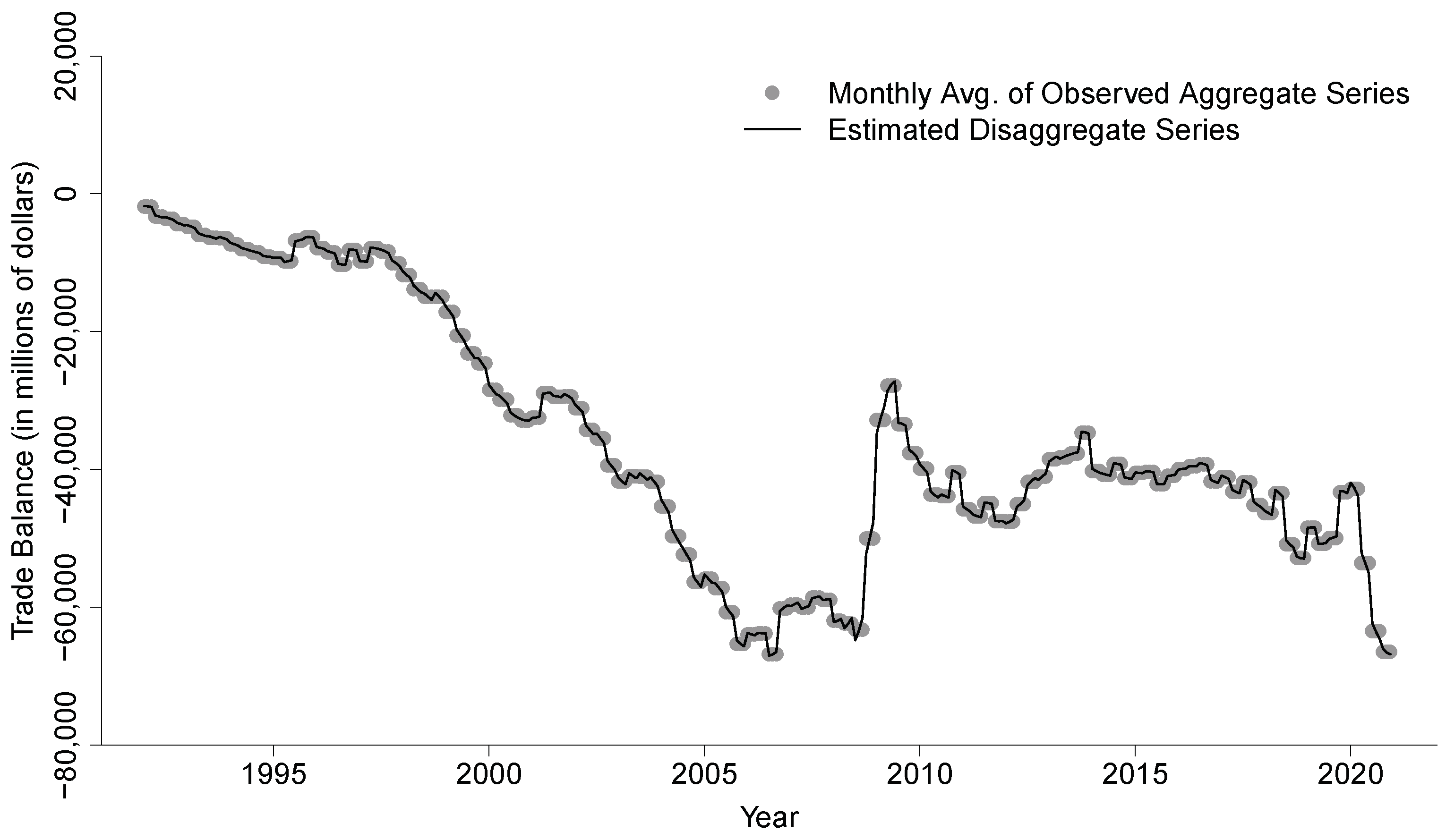
Furthermore, we calculate x ^ t , t = 1 , 2 , , 348 , using the GLS disaggregation formula of (6). The monthly disaggregate estimates x ^ t and the monthly averages of the observed aggregate series, i.e., X T / 3 , are compared in Figure 2. As illustrated in the lined graph of Figure 2, it seems obvious that x ^ t is well interpolated into the gaps between the monthly averages X T / 3 and sufficiently explains the unknown monthly pattern.
Next, we construct 95% AR-sieve bootstrap prediction intervals for the unknown monthly trade balances x t . From Steps 1 and 2 in Section 3, assuming τ = 0.001 , we select the AR ( 33 ) approximation for u ^ t = x ^ t u ^ t 1 , including the coefficient estimates
π ^ 1 = 0.81301 , π ^ 2 = 0.66099 , π ^ 3 = 0.53739 , π ^ 4 = 0.43691 , π ^ 5 = 0.35521 , π ^ 6 = 0.28879 , π ^ 7 = 0.23479 , π ^ 8 = 0.19089 , π ^ 9 = 0.15519 , π ^ 10 = 0.12617 , π ^ 11 = 0.10258 , π ^ 12 = 0.08340 , π ^ 13 = 0.06780 , π ^ 14 = 0.05513 , π ^ 15 = 0.04482 , π ^ 16 = 0.03644 , π ^ 17 = 0.02962 , π ^ 18 = 0.02408 , π ^ 19 = 0.01958 , π ^ 20 = 0.01592 , π ^ 21 = 0.01294 , π ^ 22 = 0.01052 , π ^ 23 = 0.00856 , π ^ 24 = 0.00696 , π ^ 25 = 0.00565 , π ^ 26 = 0.00460 , π ^ 27 = 0.00374 , π ^ 28 = 0.00304 , π ^ 29 = 0.00247 , π ^ 30 = 0.00201 , π ^ 31 = 0.00163 , π ^ 32 = 0.00133 , π ^ 33 = 0.00108 .
Using the AR-sieve technique presented in Step 3, we compute the empirical distribution function F ^ n ( e ˜ t ) of the centered residuals e ˜ t . The S-like shape of F ^ n ( e ˜ t ) in Figure 3 is the typical pattern of zero-mean Gaussian white noise. We remark that other AR approximation conditions, τ = 0.1 , 0.01 , and 0.0001 , are also investigated. The centered residuals for τ = 0.0001 depict a similar pattern to τ = 0.001 , while the two other conditions do not. Thus, we only consider τ = 0.001 as a predetermined positive value close to zero.
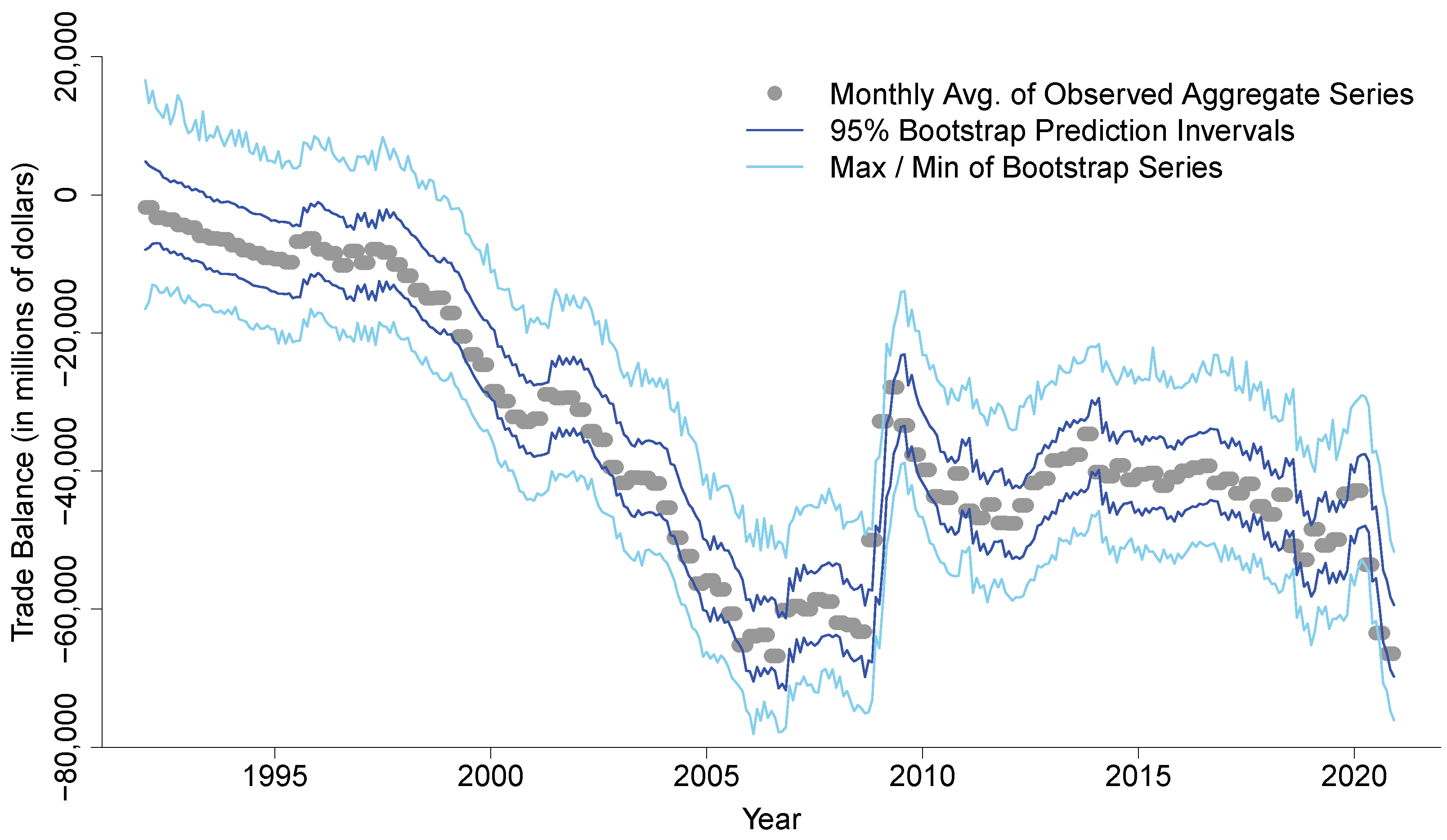
Through a large number (e.g., 25000 in our study) of consecutive iterations of Steps 4–7, we obtain the bootstrap distribution function F n ( x ^ t * ) for each bootstrap prediction x ^ t * , and we construct 95% AR-sieve bootstrap prediction intervals for all unknown x t , t = 1 , , 348 , in the form of (37). The 95% bootstrap prediction intervals of x t and the maximum and minimum x ^ t * values of F n ( x ^ t * ) for t = 1 , , 348 are drawn in Figure 4. We notice that the prediction intervals completely surround the sequence of the monthly averages X T / 3 over the indexed time and capture the exact pattern of the monthly averages. Therefore, we can conclude from Figure 4 that the AR-sieve bootstrap prediction intervals can provide reasonable bandwidths for estimation of the unknown monthly trade balances x t .

5. Concluding Remarks

In this research, we have developed a modified procedure for constructing AR-sieve bootstrap prediction intervals of an unknown disaggregate series x t . As demonstrated in Section 4, when the upper and lower limits of the prediction intervals are linked over the indexed time, we can visually outline the sequential pattern of unknown disaggregate observations within certain bandwidths. Therefore, the proposed prediction intervals can provide a measure of reliability for temporal disaggregation and account for the uncertainty in estimating x t .
In addition, the proposed method is composed of the model-based point estimation introduced in Section 2 and the nonparametric bootstrap interval estimation described in Section 3. That is, the iterative procedure of bootstrap resampling generates empirical probability distributions for unknown disaggregate observations, while a disaggregate ARIMA model is established under the assumption of Gaussian innovations. From this perspective, the proposed method can be interpreted as a semiparametric approach to estimating and predicting unknown x t values.
Our underlying assumption is that the white noise distribution is Gaussian. However, non-Gaussian time series are also frequently found in real life. For example, if a set of measurements is a time series that contains whole numbered counts, they can be modeled with a Poisson count process. Refs. [25,26,27,28] developed the generalized AR models and related estimation methods for the Poisson scenarios. In future work, as an extension of the AR-sieve method to non-Gaussian models, we will explore a wide range of possibilities of the Poisson AR-sieve bootstrap prediction intervals of temporal disaggregation. Moreover, since the current GLS and ARIMA disaggregations do not meet the non-Gaussian conditions, we will examine other model-based disaggregation methods, for example, [8,29].

Funding

This research received no external funding.

Institutional Review Board Statement

Not applicable.

Informed Consent Statement

Not applicable.

Data Availability Statement

The quarterly balances of U.S. international trade in goods and services from the first quarter of 1992 to the fourth quarter of 2020. See [23,24].

Acknowledgments

We wish to thank the Special Issue editors and reviewers for their helpful comments, which have improved the presentation of this article.

Conflicts of Interest

The author declares no conflict of interest.

References

  1. Lee, B.H.; Wei, W.W.S. The use of temporally aggregated data on detecting a mean change of a time series process. Commun. Stat. Theory Methods 2017, 46, 5851–5871. [Google Scholar] [CrossRef]
  2. Lee, B.H.; Park, J. A spectral measure for the information loss of temporal aggregation. J. Stat. Theory Pract. 2020, 14, 1–23. [Google Scholar] [CrossRef]
  3. Lee, B.H.; Wei, W.W.S. The use of temporally aggregated data in modeling and testing a variance change in a time series. Commun. Stat. Simul. Comput. 2021. Forthcoming. [Google Scholar] [CrossRef]
  4. Chow, G.C.; Lin, A. Best linear unbiased interpolation, distribution and extrapolation of time series by related series. Rev. Econ. Stat. 1971, 53, 372–375. [Google Scholar] [CrossRef]
  5. Denton, F.T. Adjustment of monthly or quarterly series to annuals totals: An approach based on quadratic minimization. J. Am. Stat. Assoc. 1971, 66, 99–102. [Google Scholar] [CrossRef]
  6. Fernández, R.B. A methodological note on the estimation of time series. Rev. Econ. Stat. 1981, 63, 471–476. [Google Scholar] [CrossRef]
  7. Litterman, R.B. A random walk, Markov model for the distribution of time series. J. Bus. Econ. Stat. 1983, 1, 169–173. [Google Scholar]
  8. Guerrero, V.M. Temporal disaggregation of time series: An ARIMA based approach. Int. Stat. Rev. 1990, 58, 29–46. [Google Scholar] [CrossRef]
  9. Stram, D.O.; Wei, W.W.S. A methodological note on the disaggregation of time series totals. J. Time Ser. Anal. 1986, 7, 293–302. [Google Scholar] [CrossRef]
  10. Wei, W.W.S.; Stram, D.O. Disaggregation of time series models. J. R. Stat. Soc. Ser. Stat. Methodol. 1990, 52, 453–467. [Google Scholar] [CrossRef]
  11. Feijoó, S.R.; Caro, A.R.; Quintana, D.D. Methods for quarterly disaggregation without indicators: A comparative study using simulation. Comput. Stat. Data Anal. 2003, 43, 63–78. [Google Scholar] [CrossRef]
  12. Moauro, F.; Savio, G. Temporal disaggregation using multivariate structural time series models. Econom. J. 2005, 8, 214–234. [Google Scholar] [CrossRef] [Green Version]
  13. Sax, C.; Steiner, P. Temporal disaggregation of time series. R J. 2013, 5, 80–87. [Google Scholar] [CrossRef] [Green Version]
  14. Alonso, A.M.; Pẽna, D.; Romo, J. Forecasting time series with sieve bootstrap. J. Stat. Plan. Inference 2002, 100, 1–11. [Google Scholar] [CrossRef] [Green Version]
  15. Alonso, A.M.; Pẽna, D.; Romo, J. On sieve bootstrap prediction intervals. Stat. Probab. Lett. 2003, 65, 13–20. [Google Scholar] [CrossRef] [Green Version]
  16. Alonso, A.M.; Sipols, A.E. A time series bootstrap procedure for interpolation intervals. Comput. Stat. Data Anal. 2008, 52, 1792–1805. [Google Scholar] [CrossRef]
  17. Stram, D.O.; Wei, W.W.S. Temporal aggregation in the ARIMA process. J. Time Ser. Anal. 1986, 7, 279–292. [Google Scholar] [CrossRef]
  18. Wei, W.W.S. Time Series Analysis: Univariate and Multivariate Methods, 2nd ed.; Addison Wesley: Boston, MA, USA, 2006. [Google Scholar]
  19. Wei, W.W.S. Seasonal Analysis of Economic Time Series; CHAPTER Some Consequences of Temporal Aggregation in Seasonal Time Series Models; U.S. Department of Commerce, Bureau of the Census: Washington, DC, USA, 1978; pp. 433–444.
  20. Box, G.E.P.; Jenkins, G.M.; Reinsel, G.C.; Ljung, G.M. Time Series Analysis: Forecasting and Control, 5th ed.; John Wiley & Sons: Hoboken, NJ, USA, 2016. [Google Scholar]
  21. Brockwell, P.J.; Davis, R.A. Time Series: Theory and Methods, 2nd ed.; Springer: New York, NY, USA, 2006. [Google Scholar]
  22. U.S. Census Bureau Economic Indicators. Available online: https://www.census.gov/economic-indicators (accessed on 28 February 2021).
  23. U.S. International Trade Data. Available online: https://www.census.gov/foreign-trade/data/index.html (accessed on 13 February 2021).
  24. International Trade in Goods and Services. Available online: https://www.bea.gov/data/intl-trade-investment/international-trade-goods-and-services (accessed on 13 February 2021).
  25. Freeland, R.K.; McCabe, B.P.M. Analysis of low count time series data by Poisson autoregression. J. Time Ser. Anal. 2004, 25, 701–722. [Google Scholar] [CrossRef]
  26. Fokianos, A.; Rahbek, A.; Tjøstheim, D. Poisson autoregression. J. Am. Stat. Assoc. 2009, 104, 1430–1439. [Google Scholar] [CrossRef] [Green Version]
  27. Zhu, F.; Wang, D. Estimation and testing for a Poisson autoregressive model. Metrika 2011, 73, 211–230. [Google Scholar] [CrossRef]
  28. Chen, C.W.S.; Lee, S. Generalized Poisson autoregressive models for time series of counts. Comput. Stat. Data Anal. 2016, 99, 51–67. [Google Scholar] [CrossRef]
  29. Hotta, L.K.; Vasconcellos, K.L. Aggregation and disaggregation of structural time series models. J. Time Ser. Anal. 1999, 20, 155–171. [Google Scholar] [CrossRef]
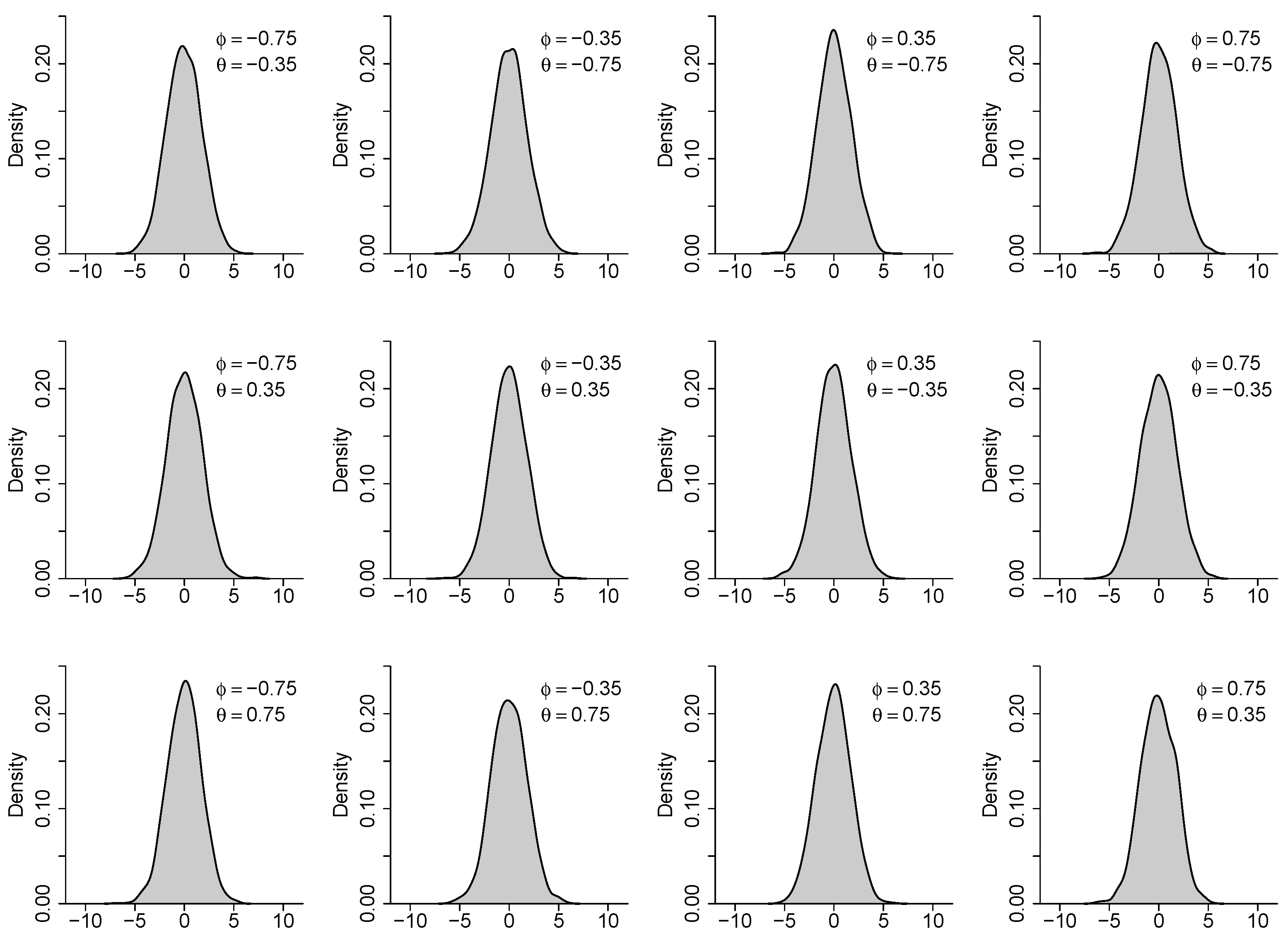
Figure 1. Density plots of bootstrap resamples of size 5000 for the centered residuals e ˜ t .
Stats 05 00013 g001
Figure 2. Monthly averages of the observed aggregate series vs. estimated disaggregate series.
Stats 05 00013 g002
Figure 3. Empirical cumulative distribution function of the centered residuals e ˜ t .
Stats 05 00013 g003
Figure 4. Bootstrap prediction intervals for the unknown monthly series x t .
Stats 05 00013 g004
Table 1. Mean values, standard deviations, and the Shapiro–Wilk test results for the bootstrap resamples drawn in Figure 1.
ϕ θ MeanSdW-Statisticp-Value
0.75 0.35 0.03279 1.73068 0.99247 0.61783
0.75 0.35 0.00814 1.78736 0.99271 0.64584
0.75 0.75 0.00993 1.67396 0.99321 0.70362
0.35 0.75 0.00597 1.80319 0.99254 0.62554
0.35 0.35 0.00768 1.73869 0.99416 0.80999
0.35 0.75 0.00223 1.75250 0.99419 0.81240
0.35 0.75 0.03641 1.68577 0.99342 0.72751
0.35 0.35 0.01750 1.74479 0.99294 0.67239
0.35 0.75 0.05127 1.69289 0.99169 0.53010
0.75 0.75 0.02573 1.76438 0.99207 0.57279
0.75 0.35 0.01051 1.79086 0.99271 0.64575
0.75 0.35 0.05146 1.71417 0.99310 0.69043
Table 2. The BIC values of the fitted ARMA ( p , q ) models of V T for p and q = 0 , 1 , , 10 .
p = 0 12345678910
q = 0 2458.10 2447.40 2447.39 2451.29 2449.77 2454.26 2458.19 2461.61 2466.23 2470.66 2475.38
1 2439.75 2443.08 2447.79 2452.52 2454.36 2457.65 2462.10 2466.14 2470.88 2475.40 2479.71
2 2443.21 2447.80 2452.57 2456.98 2458.48 2462.05 2467.14 2467.64 2475.63 2480.12 2480.09
3 2447.81 2452.51 2457.18 2457.58 2462.46 2466.70 2471.40 2471.63 2476.32 2480.10 2480.64
4 2452.25 2456.36 2458.65 2462.00 2466.64 2471.14 2475.81 2472.15 2476.98 2484.85 2484.58
5 2454.33 2459.07 2462.15 2466.71 2471.48 2473.01 2479.69 2476.58 2481.51 2484.40 2489.01
6 2459.07 2462.63 2466.64 2471.28 2475.10 2479.20 2482.06 2486.42 2489.60 2489.12 2493.61
7 2462.52 2466.53 2471.24 2475.55 2476.00 2482.14 2486.52 2485.05 2494.68 2500.22 2498.04
8 2466.27 2470.60 2473.06 2476.34 2480.72 2486.30 2487.91 2490.70 2497.10 2498.50 2503.03
9 2470.83 2475.26 2480.07 2480.91 2485.65 2490.12 2494.56 2495.01 2496.75 2505.48 2510.27
10 2474.49 2479.21 2483.43 2484.44 2488.40 2492.39 2497.26 2497.14 2501.86 2503.55 2509.34
Publisher’s Note: MDPI stays neutral with regard to jurisdictional claims in published maps and institutional affiliations.