Quantitative Trading through Random Perturbation Q-Network with Nonlinear Transaction Costs

Abstract

In recent years, reinforcement learning (RL) has seen increasing applications in the financial industry, especially in quantitative trading and portfolio optimization when the focus is on the long-term reward rather than short-term profit. Sequential decision making and Markov decision processes are rather suited for this type of application. Through trial and error based on historical data, an agent can learn the characteristics of the market and evolve an algorithm to maximize the cumulative returns. In this work, we propose a novel RL trading algorithm utilizing random perturbation of the Q-network and account for the more realistic nonlinear transaction costs. In summary, we first design a new near-quadratic transaction cost function considering the slippage. Next, we develop a convolutional deep Q-learning network (CDQN) with multiple price input based on this cost functions. We further propose a random perturbation (rp) method to modify the learning network to solve the instability issue intrinsic to the deep Q-learning network. Finally, we use this newly developed CDQN-rp algorithm to make trading decisions based on the daily stock prices of Apple (AAPL), Meta (FB), and Bitcoin (BTC) and demonstrate its strengths over other quantitative trading methods.

1. Introduction

Reinforcement learning (RL) is revolutionizing modern society in many areas including robotics [1], games [2], economics [3], science [4], healthcare [5], and everyday life, bringing the sci-fi notion of artificial intelligence (AI) to reality step by step. RL also started to see applications in quantitative trading algorithms for better trade decisions [6]. Traditionally, traders built mathematical models to monitor business news and trading activities in real-time to detect any factors that can force security prices to rise or fall. Such model comes with a predetermined set of instructions on various parameters including timing, price, quantity, and other factors, for placing trades automatically without the trader’s active involvement. Unlike human traders, quantitative trading can simultaneously analyze large volumes of data and make thousands of trades every day. RL learns the trading decisions from the reward and makes fast trading decisions, rendering superior performance over the market average.

As a unique frontier of machine learning, RL provides a framework for autonomous learning and decision-making for control problems. The agent in RL learns a policy concerned with how to take actions in an environment to maximize the cumulative reward (Sutton and Barto, 2018) [7]. In quantitative trading, Moody and Saffell (1998) [8] proposed the pioneering work using recurrent reinforcement learning to train the trading systems. The recurrent network that they used, however, is too simple to capture the market movement. In recent years, significant progress has been made by combining advances in deep learning with RL, resulting in the “Deep Q-network” (DQN) algorithm (Mnih et al., 2015) [9], capable of human level performance on tasks such as image processing. The ability to quickly search for hidden patterns and learn control policies from high-dimensional data (LeCun, Bengio and Hinton, 2015) [10] renders DQN widely applicable to many fields other than image processing.

In quantitative trading, transaction costs are important to investors because they are a key determinant of net returns. The average annual transaction cost for a mutual fund in the U.S. was estimated at 1.44% (Edelen, et al., 2013) [11]. The first part of these costs is brokerage commissions and taxes from when a fund manager buys or sells a stock. One possible way to pay less brokers’ fees is to invest in lower-turnover funds using the buy-and-hold strategy for actively managed fund (Edelen, et al., 2007) [12]. The second part of the costs is the slippage which primarily comes from the $\alpha$ decay and bid/ask spread. The spread cost can be greater if the securities have less liquidity or are traded across global exchanges. A large mutual fund may also incur market impact costs when the fund’s sizable purchase of stock drives the price higher artificially. These costs can be diminished by spreading the purchases over longer periods of time.

For the linear transaction cost model, nontrade region can be obtained using an augmented quadratic programming (Scherer, 2007) [13]. As mentioned by Lecesne and Roncoroni (2019) [14], unit transaction costs may be a linear function of the trading size according to the supply–demand curve. The linear term describes the price deviation from the intended price entailed by a trade quantity under liquidity frictions, implying that a trading model with quadratic transaction costs may be more appropriate. Due to the nonlinearity nature of the transaction cost function, the ordinary linear programming or quadratic programming techniques commonly used in portfolio optimization cannot be applied. Until recently, the mean–variance optimized portfolios with quadratic transaction costs are usually obtained using quadratic programming and the alternating direction method of multipliers (Chen, 2020) [15]. To date, other transaction cost functions have yet to be studied. Under the RL framework, however, it is possible to consider flexible transaction cost functions in quantitative trading.

In a real financial market, unpredictable stock prices and socioeconomic events often lead to noisy and nonstationary financial data, rendering the prediction of trading behaviors arduous. In quantitative trading, the most widely used method is technical analysis (Murphy 1999) [16] first introduced by Charles Dow as part of the Dow Theory in the late 1800s. It builds technical indicators using predominantly charts of Opening-High-Low-Closing prices (OHLC) and trading volumes, and identifies trading opportunities by analyzing statistical trends gathered from these trading activities. Technical analysts view past trading activity activities and price changes valuable indicators of a security’s future price movements, which can in turn be embedded into a current reinforcement learning framework for trading.

The remaining part of this paper is organized as follows. In Section 2, we introduce the basic RL framework and the reward function used in finance. In Section 3, we then propose the convolutional deep Q-network with random perturbation (CDQN-rp) associated with nonlinear transaction costs to address the aforementioned challenges. In particular, for the first challenge concerning all kinds of transaction costs, we establish our own near-quadratic model in Section 3.1 to include the effect of slippage, especially the bid/ask spread and market impact, as well as the fixed explicit costs. For the second challenge regarding integrating technical analysis to reinforcement learning, we first stack n consecutive prices as a single input, and then utilize the convolutional layers on top of the DQN, as introduced in Section 3.2 and Section 3.3. For the last challenge of instability and overoptimistic estimation issues behind training DQN, we develop the random perturbation policy network method in Section 3.4, which can also be embedded into the double Q-learning. In Section 4, we develop trading strategies for several stocks using the newly proposed RL method and compare its performance to other baseline trading strategies to demonstrate the strength of our new method in terms of higher cumulative wealth and Sharpe ratio.

2. Reinforcement Learning Structure

2.1. Markov Decision Process

The Markov decision processes (MDP) is a mathematically idealized form of the reinforcement learning (RL) problem for which interaction is used to achieve a goal. The decision maker, or the agent, and the environment interact at each of the discrete time steps, $t=0,1,2,3\dots$. At each time step t, there is a corresponding state $S_t$ representing the condition of the environment, and the agent selects an action $A_t$ accordingly. One time step later, based on the action selected, the agent immediately receives a reward $R_{t+1}$, and the environment moves to a new state $s_{t+1}$. The MDP and the agent together generates a sequence of trajectory:

$$S_0,A_0,R_1,S_1,A_1,R_1,S_2,A_2,R_3,\dots$$

The goal of the RL is to maximize the total amount of reward, namely the cumulative reward in the long run, the agent receives. In particular, the agent chooses $A_t$ to maximize the expected discounted reward (if $\gamma =1$, it means no discount):

$$G_t=R_{t+1}+\gamma R_{t+2}+{\gamma }^2{R}_{t+3}+...=\sum _{k=0}^{\infty }{\gamma }^k{R}_{t+k+1}$$

(1)

where $\gamma$ is the discount rate, ranging from 0 to 1.

2.2. Action–Value Functions and Q-Learning

In order to estimate “how good” a certain state–action pair (a given action in a given state) is, RL involves value functions to evaluate the state–action pair. An action–value function is defined with respect to a certain policy $\pi$, which is a mapping from the state–action pairs to their probabilities. Define the action–value function for policy $\pi$ of taking action a in state s by $q_{\pi }(s,a)$, as the expected return starting from s, taking action a, and, thereafter, following policy $\pi$:

$$q_{\pi }(s,a)={\mathbb{E}}_{\pi }[\sum _{k=0}^{\infty }{\gamma }^k{R}_{t+k+1}|S_t=s,A_t=a]$$

(2)

The optimal policies share the same optimal action–value function $q_{*}$:

$$q_{*}(s,a)=\underset{\pi }{max}{q}_{\pi }(s,a)$$

(3)

To estimate the true optimal value function, an early breakthrough in RL was the development of an off-policy temporal difference control algorithm known as the Q-learning algorithm (Watkins, 1989) [17] to iteratively update the estimation of $q_{*}$:

$$Q(S_t,A_t)\leftarrow (1-\alpha )Q(S_t,A_t)+\alpha [R_{t+1}+\gamma \underset{a}{max}Q(S_{t+1},a)]$$

(4)

where $Q(s,a)$ denotes the estimation of $q_{*}(s,a)$.

2.3. Additive Profits, Multiplicative Profits and Sharpe Ratio

There are mainly two types of profits: the additive profit and the multiplicative profit. The additive profit is appropriate to consider if each trade is for a fixed number of shares or contracts of security $s_t$. With the definitions $r_t=s_t-s_{t-1}$ and $r_t^f$ for the price returns of a risky (traded) asset and a risk-free asset (such as T-Bills), respectively, the additive profit accumulated over T time periods with trading position size $\mu >0$ is then defined as:

$$\begin{array}{cc}\hfill P_T=& P_0+\sum _{t=1}^T{R}_t\hfill \\ \hfill =& \hfill P_0+\mu \sum _{t=1}^T(r_t^f+A_{t-1}(r_t-r_t^f)-C_t)\hfill \end{array}$$

(5)

where $A_{t-1}$ is the position held at time $t-1$ and $C_t$ is the transaction costs at time t, with $P_0=0$ and typically $A_T=A_0=0$. Equation (1) holds for continuous quantities also. The wealth is defined as $W_T=W_0+P_T$.

The multiplicative profit is appropriate when a fixed fraction of accumulated wealth $\nu >0$ is invested in each long or short trade. Here, $r_t=\frac{s_t}{s_{t-1}}-1$. If no short sales are allowed and the leverage factor is set fixed at $\nu =1$, the wealth at time T is:

$$\begin{array}{cc}\hfill W_T=& W_0\prod _{t=1}^T(1+R_t)\hfill \\ \hfill =& \hfill W_0\prod _{t=1}^T(1+(1-A_{t-1})r_t^f+A_{t-1}{r}_t)(1-C_t)\hfill \end{array}$$

(6)

Instead of maximizing the profit alone, most hedge fund managers attempt to maximize the profit with risk adjusted. The Sharpe ratio is the most widely used measure of risk adjusted return. The Sharpe ratio $S{R}_t$ for period $t=\{1,2,\dots ,T\}$ with returns $R_t$ is defined as follows:

$$S{R}_t=\frac{\mathrm{Mean}\left(R_t\right)}{\mathrm{Standard}\mathrm{Deviation}\left(R_t\right)}$$

(7)

3. Methodology

3.1. Transaction Cost Model

Quantitative traders use transaction cost models to have reasonable expectations for the possible cost of an order which they will trade and adjust their trading strategies accordingly. There are four basic transaction cost models: flat, linear, piecewise linear, and quadratic. For theoretical quantitative methods utilizing stochastic processes and partial differential equations, transaction costs are often ignored. For most machine learning methods such as neural networks and especially those for time series data such as the long short term memory (LSTM), either fixed transaction costs or linear transaction costs are considered. In the framework of reinforcement learning (RL), the structure of the transaction costs can be flexible, rendering it feasible to use quadratic or even more complex functions, which are often more suitable and realistic.

In reality, transaction costs include not only the explicit costs, but also the slippage and opportunity cost which are harder to model. Some costs such as commissions, fees, and taxes are fixed, while other costs, such as slippage and opportunity cost, cannot be known precisely before a trade is completed. Slippage refers to situations in which a trader receives a different trade execution price than intended. Slippage can be caused by several factors, such as the volatility, the order size, or even abrupt change in the bid/ask spread. For small orders, slippage is primarily caused by bid/ask spread, while for large orders, slippage is often due to the market impact. Market impact can also be affected by many drivers, including the size of the order being executed and the liquidity of the instrument. One way to avoid unexpected slippage is to set the price limits or conditional execution strategies, which, in turn, may cause the opportunity cost. Unlike other factors of the transaction costs occurring when an order is executed, the opportunity cost refers to the potential loss from unexecuted shares.

Since we evaluate and adjust our position each trading day, our quantitative trading framework belongs to low frequency trading according to the daily strategy holding period. We use the following factor equation to model the slippage and market impact:

$$\mathrm{expected\; price\; =\; baseline\; price\; +/}-\left[f\right(spread)+g(size,volatility\left)\right]$$

where expected price refers to the actual realized price rather than the intended trading price if a trading is completed, “+/−” is determined by the side (“+” for buy side while “−” for sell side).

The baseline price used in our model is the $current$ $price$. The $spread$ cost is 4 basis points and the basic spread function is $f\left(spread\right)=0.5\times spread$. The last market impact term is set to be $g(size,volatility)\propto siz{e}^{\alpha }\times volatility$, where $\alpha$ is a constant close to but less than 1. Some possible choices of $\alpha$ are 0.88, 0.92, and 0.96 to satisfy the mathematical requirements of a fractional exponents. For simplicity, we currently do not consider the price limits; thus no opportunity cost is needed. Furthermore, to estimate the local volatility, we utilize the $volatility\propto current$ $price$ approximation. The expected price in our model is therefore:

$$\mathrm{expected\; price}=s_t+/-[0.5\times 0.0004+\delta \times siz{e}^{0.92}\times s_t]$$

where $\delta$ is a pre-determined scalar and $s_t$ is the current price.

Most work to date uses the linear transaction model in their quantitative trading setting. Considering different underlying factors such as slippage and market impact mentioned above, the transaction cost should behave nonlinearly in terms of the size, as the realized price itself is a function of size. Therefore, in our quantitative trading framework, we use a more realistic near-quadratic approximation to model the transaction cost $C_t$ at time t, with the size determined by the position change when unit share assumption holds:

$$\begin{array}{cc}\hfill C_t& =(\mathrm{expected}\mathrm{price}-s_t)\times size\hfill \\ \hfill & =+/-[0.0002\times size+\delta \times siz{e}^{1.92}\times s_t]\hfill \\ \hfill & =\delta {(A_t-A_{t-1})}^{1.92}{s}_t+(A_t-A_{t-1})\times 0.0002\hfill \end{array}$$

(8)

3.2. Stacked Prices State

At each time step t, we consider the price of a single security with price series $s_t$. Instead of using a single price $s_t$ as our state, we consider a tuple $S_t$: $S_t=(s_{t-n+1},s_{t-n+2},\dots ,s_{t-1},s_t)$ with consecutive n prices as our current state at time t. The reason behind stacking a few consecutive stock prices to represent a single state, lie in that the impact of uncertainty is cumulative and dependent upon the history of the process, and not merely its current value. A single price will not be enough for our network to fully understand the state of an environment. By looking at one single price without the historical trajectory, it is impossible to tell whether the price will rise or fall the next day. Moreover, one single price cannot reveal the “speed” of the price movement. If we set the n consecutive prices as the current state instead, the network will have a much better understanding of the current state of the environment.

One advantage of using stacked price states is that the historical information is automatically included when we input the state into the network for learning. Therefore, no recurrent layer is needed, and all layers can be feedforward, which reduces the computational complexity, as computational cost of a recurrent model grows with the number of time steps the model needs to go through [18].

The action space in our setting contains three values: −1, 0, 1, representing the three possible positions we hold for a particular security—short, neutral, or long position, respectively. The trader is assumed to take the position $A_t$ at a constant magnitude. To enable risk control, this assumption can be easily relaxed. The position $A_t$ is determined at time t and reassessed at time $t+1$. The reward $R_t$ is calculated using additive profits due to the constant magnitude assumption. The summary of our MDP formulation is as follows:

Markov Decision Process Setting: State space: $S_t=(s_{t-n+1},s_{t-n+2},\dots ,s_{t-1},s_t)$ Action space: $A_t\in \{-1,0,1\}$ (short, neutral, long); Discount rate: $\gamma =e^{-r^f\Delta t}$, which is the continuous discount factor; Rewards: $R_t=r_t^f+(s_t-s_{t-1}-r_t^f)A_{t-1}-\delta {(A_t-A_{t-1})}^{1.92}{s}_t-0.0002(A_t-A_{t-1})$.

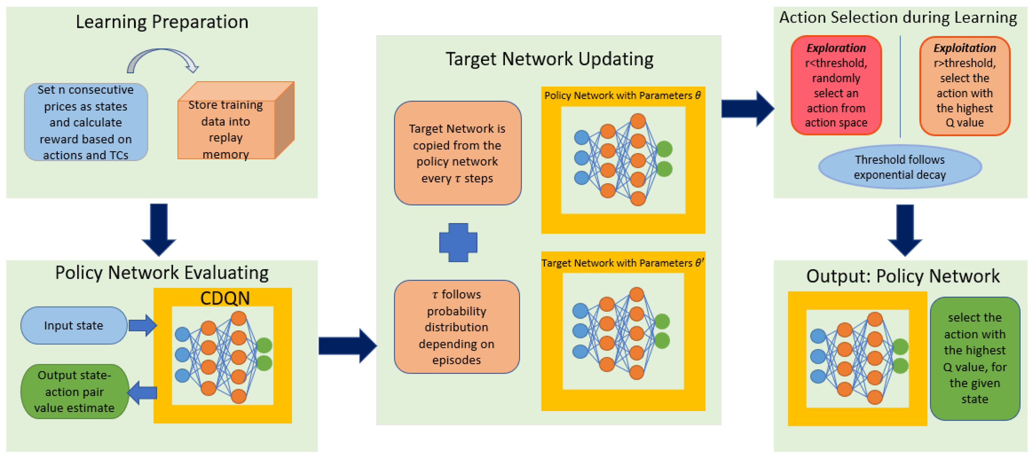
3.3. Convolutional Deep Q-Learning Network

DQN combines Q-learning with a flexible deep neural network with the potential for a low asymptotic approximation error, reducing noise in the environment significantly, and therefore producing the best-case scenario for Q-learning in some ways (Van Hasselt et al., 2016) [19]. The input of the network is the current state while the output vector is the action value estimate associated with the input state and all possible actions.

Convolutional neural networks (CNNs) are primarily used in the field of pattern recognition, such as image processing, because the convolutional layers are particularly designed for edge detection and impulse response filters (O’Shea, 2015) [20]. Besides fully connected layers, CNNs also include convolutional layers and pooling layers. Adding convolutional layers on top of DQN will produce the CDQN framework for RL. Through transformation, CDQNs can analyze the original input trajectory, layer by layer, using convolutional and down sampling techniques to detect the “trading signals” automatically, without applying technical analysis to build and extract signals manually.

The convolution output for one stacked price sequence in the convolutional layer is calculated according to the following equation:

$$y\left(h\right)=(x\ast w)\left[h\right]=\sum _{k}x\left(k\right)\times w(h-k)$$

(9)

where y is the convolution output in the next layer, x is the input stacked prices, w is the kernel matrix, and ∗ is the convolution operator.

Apart from the convolutional layers, pooling layers are always included in the CNNs. The aim of the pooling layer is to reduce the complexity cost through decreasing the dimensionality of the input gradually. In our CDQN framework, the max-pooling layers with kernels of a dimensionality of 2 × 2 are implemented. Another advantage of adding the pooling layer is to render the model invariant to some noises and thus capture the true trading signals.

3.4. Deep Q Networks with Random Perturbation

To train the network, the Bellman optimality equation is used to obtain the target Q-values:

$$Q^{target}(s,a)=R_{t+1}+\gamma \underset{a^{\prime }}{max}Q(s^{\prime },a^{\prime })$$

(10)

For the gradient in DQN, the loss between the output Q-values and the target Q-values needs to be calculated. The latter, target Q-values, require a second pass to the same DQN, known as the policy network, with the next state $s^{\prime }$ as input. The same weights used to update both the output Q-values and the target values will lead the optimization process to the “chasing tail” instability, as the output Q-values move closer to their targets while the targets move further away. One solution proposed by Mnih and colleagues (2015) is to obtain the target Q-values from a separate network, aptly named the target network.

The target network is a clone of the policy network. Its weights are frozen except for that, periodically, after every certain number of time steps $\tau$, the weights are copied from the policy network’s new weights. If we denote the policy network’s parameters by $\theta$, for a given state s, the DQN outputs a vector of action values $Q(s,·;\theta )$ using the policy network. The target Q-values calculated from the target network with parameters ${\theta }^{\prime }$ is then determined by:

$$Q^{target}=R_{t+1}+\gamma \underset{a^{\prime }}{max}Q(S_{t+1},a^{\prime };{\theta }_t^{\prime })$$

(11)

where ${\theta }_t^{\prime }={\theta }_{t+1}^{\prime }=\dots ={\theta }_{t+\tau -1}^{\prime }={\theta }_t$ and ${\theta }_{t+\tau }^{\prime }={\theta }_{t+\tau +1}^{\prime }=\dots ={\theta }_{t+2\tau -1}^{\prime }={\theta }_{t+\tau }$, as shown in Figure 1.

The choice of predetermined $\tau$ can influence the speed of the convergence, i.e., the number of episodes needed to reach the optimal value. If $\tau$ is large, which means that the weights of the target network ${\theta }^{\prime }$ are fixed for many steps, then the selection process $\underset{a^{\prime }}{argmax}Q(s_{t+1},a^{\prime };{\theta }^{\prime })$ may not be up-to-date, especially at the beginning of the learning. If $\tau$ is small, however, indicating that the weights of the target network ${\theta }^{\prime }$ are changed frequently, then the instability issue may appear again. Even though cross-validation can be applied to tune a single “best” $\tau$ in a specific situation, the value of $\tau$ should behave differently at different learning phases, not to mention the complexity cost of the tuning process.

We now consider a random variable $\tau$ instead of a deterministic $\tau$, and let $\tau \left(i\right)$ be a function of learning episodes. In general, $\tau \left(i\right)$ follows a stochastic process $D\left(i\right)$ with discrete probability distributions. Define the values which $\tau \left(i\right)$ can take by $V_i=\{v_{i_1},v_{i_2},\dots ,v_{i_{n\left(i\right)}}\}$ with $v_{i_1}<v_{i_2}<\dots <v_{i_{n\left(i\right)}}$. At the beginning of the learning phase, i.e., when i is relatively small, $\tau \left(i\right)$ should, to some extent, take small values as the weights change significantly at the start, so that $P(\tau \left(i\right)=v_{i_1})>P(\tau \left(i\right)=v_{i_2})>\dots >P(\tau \left(i\right)=v_{i_{n\left(i\right)}})$. When the learning is near the end, i.e., when t is relatively large, $\tau \left(i\right)$ should take large values instead as the weights become more and more stable, so that $P(\tau \left(i\right)=v_{i_1})<P(\tau \left(i\right)=v_{i_2})<\dots <P(\tau \left(i\right)=v_{i_{n\left(i\right)}})$. During the middle part of learning, $\tau \left(i\right)$ can take uniform distribution so $P(\tau \left(i\right)=v_{i_1})=P(\tau \left(i\right)=v_{i_2})=\dots =P(\tau \left(i\right)=v_{i_{n\left(i\right)}})$. Some advantages of a random $\tau \left(i\right)$ are: (i) the network will not stuck at the local optimum compared to a fixed $\tau$, (ii) no tuning process is needed, which saves the computational cost. Under this setting, the new target network behaves like a random perturbation of the original policy network. Figure 2 shows our proposed CDQN-rp algorithm of applying the CDQN with random perturbation (rp) method in quantitative trading. Below is the detailed algorithm for updating ${\theta }^{\prime }$ based on the random perturbation policy network.

We assume the total number of episodes for learning is N and the total time step for one episode is T. For a specific episode i, do the following steps:

• Step 1: initialize ${\theta }_0$, and set ${\theta }_0^{\prime }={\theta }_0$ and $t_{cum}=0$;
• Step 2: generate $\tau =\tau \left(i\right)$ according to the following probability mass function, where the constant $c(c\ge 1)$ controls the “tendency” of uniform weights, as all $v_{i_k}$s have the same weights when $c\stackrel{}{\to }\infty$, while $v_1$ or $v_{n\left(i\right)}$ (depending on i) will have the weight close to 1 when $c\stackrel{}{\to }1$:

  $$\begin{array}{cc}\hfill P(\tau =v_{i_k})& =\frac{exp(v_{n\left(i\right)-k+1}/c)}{{\displaystyle \sum _{j=1}^{n\left(i\right)}}exp(v_{i_j}/c)},\mathrm{if}i\le \lfloor \frac{N}{3}\rfloor ;\hfill \\ P(\tau =v_{i_k})\hfill & =\frac{1}{n\left(i\right)},\mathrm{if}\lfloor \frac{N}{3}\rfloor \le i\le \lfloor \frac{2N}{3}\rfloor ;\hfill \\ P(\tau =v_{i_k})\hfill & =\frac{exp(v_{i_k}/c)}{{\displaystyle \sum _{j=1}^{n\left(i\right)}}exp(v_{i_j}/c)},\mathrm{if}i>\lfloor \frac{2N}{3}\rfloor .\hfill \end{array}$$
• Step 3: update ${\theta }_t$ via deep Q network while keep ${\theta }_t^{\prime }={\theta }_{t_{cum}}$ for all $t_{cum}<t<max\{\tau +t_{cum},NT+1\}$;
• Step 4: update $t_{cum}=t_{cum}+\tau$ and set ${\theta }_t^{\prime }={\theta }_{t_{cum}}$ when $t=t_{cum}$
• Step 5: repeat Step 2 to Step 4 until $t_{cum}\ge NT$.

The max operator in standard Q-learning and DQN uses the same weights to select and to evaluate a given action, resulting in overestimated values, as pointed out by van Hasselt and colleagues (2016). Double Q-learning using two value functions with two sets of weights, $\theta$ and ${\theta }^{double}$, is proposed to prevent the overoptimistic value estimates. The experiences are randomly assigned to update one of the two sets of weights. One set of weights $\theta$ is used to select the greedy action while the other set of weights ${\theta }^{double}$ is used to evaluate the value. For a clear comparison, the target Q-values in DQN can be rewritten as:

$$Q^{target}=R_{t+1}+\gamma Q(S_{t+1},\underset{a^{\prime }}{argmax}Q(S_{t+1},a^{\prime };\theta );\theta )$$

(12)

The target Q-values in Double DQN can be written as:

$$Q^{double}=R_{t+1}+\gamma Q(S_{t+1},\underset{a^{\prime }}{argmax}Q(S_{t+1},a^{\prime };\theta );{\theta }^{double})$$

(13)

Similar to the random perturbation policy network, ${\theta }^{double}$ can take the same values as ${\theta }^{\prime }$ defined above without sacrificing part of the data to build a different network. Therefore, the random perturbation result can be directly applied to double Q-learning as well.

4. Experimental Results

4.1. General Context

A long/short trading system is trained using various trading strategies including the newly proposed CDQNn-rp (convolutional deep Q-network with random perturbation) algorithm, and based on the daily prices of stocks and cryptocurrency—AAPL (Apple Inc.), FB (Meta Platforms, Inc.), and BTC (Bitcoin) from January 2017 to December 2021 while utilizing the 4- week Treasury Bill data to help maximize the cumulative rewards. The Treasury Bill is served as the risk-free asset. If we do not hold a long position on the risky asset, we invest our money in the risk-free asset. The prediction results are compared using different trading strategies for the year 2021. All data were downloaded freely from Google Finance (https://www.google.com/finance/?hl=en, accessed on 17 March 2022) and the Min-max normalization is used to preprocess the data. The real data experiments are divided into two parts. The first is to compare the total cumulative wealth and the Sharpe ratio using different trading strategies, based on a single stock or cryptocurrency. The second part is to demonstrate that our new random perturbation technique can indeed improve the learning results in terms of both cumulative wealth and Sharpe ratio. The hyper-parameters used in the experiments are shown in Appendix A 

Table A1. The hyper-parameters used in CDQNrp and LSTM in real data experiments.

Hyper-Parameters	Value
batch size	64
replay memory size	100,000
target network update frequency $\tau$	5000, 8000, 10,000, 20,000
uniform tendency c	5000
learning rate	0.00025
initial exploration	1
final exploration	0.01
decay rate	0.00025
number of episodes	1000
LSTM forecast	one-step ahead
LSTM input units	50

.

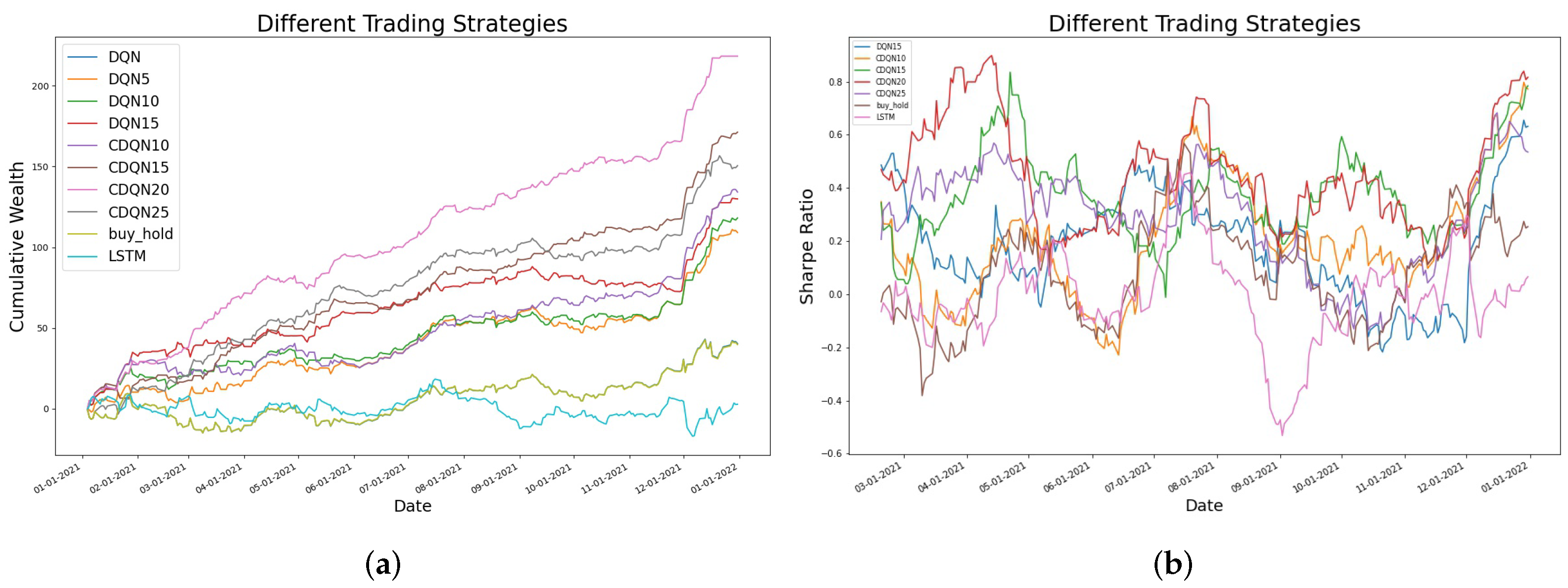
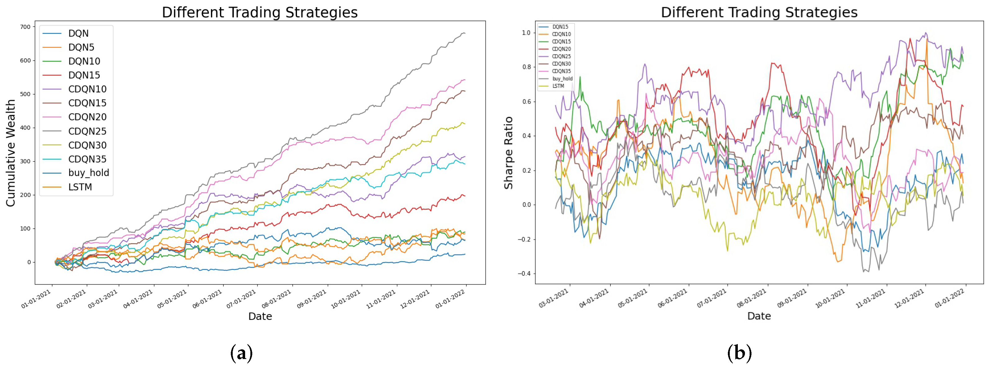
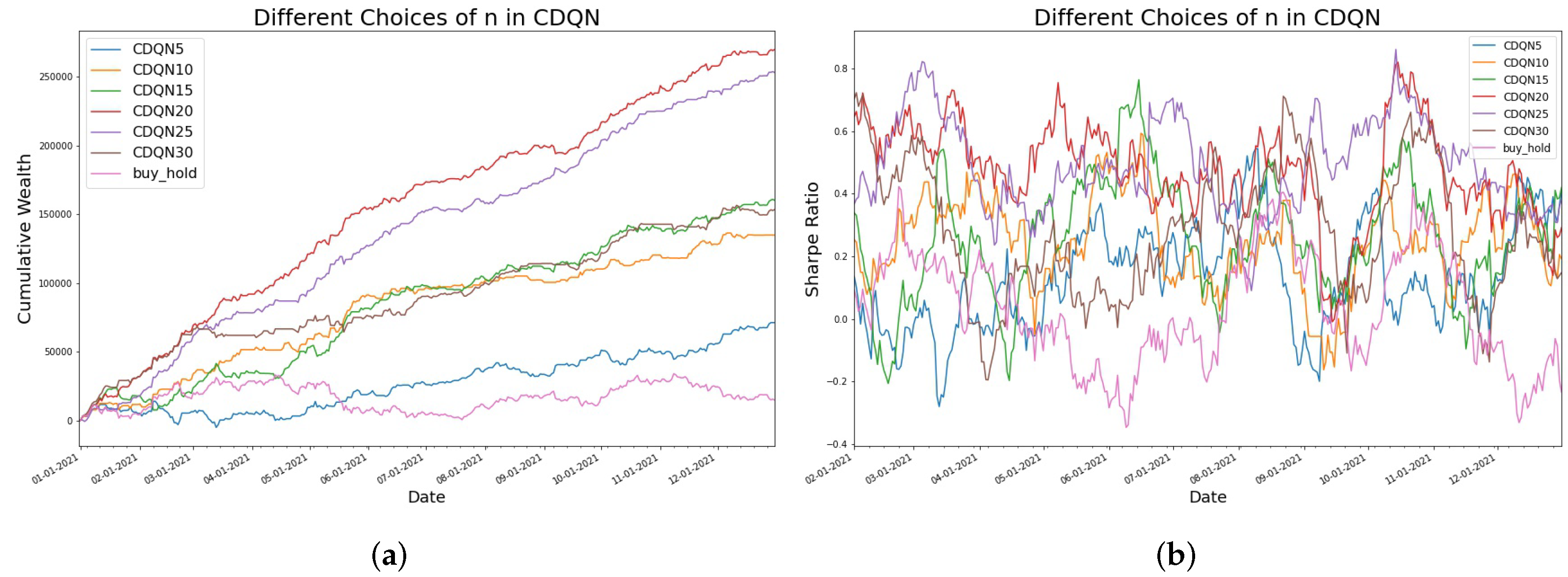
4.2. Different Trading Strategies in Cumulative Wealth and Sharpe Ratio

The following trading strategies are compared:

Buy and Hold: traditional buy and hold strategy LSTM: trading based on LSTM predictions DQN: naive deep Q-network with single stock price DQNn: deep Q-network with n consecutive daily prices CDQNn: convolutional deep Q-network with n consecutive daily prices CDQNn_rp: convolutional deep Q-network with n consecutive daily prices, trained with random perturbation target network

For reinforcement learning (RL) based strategies, namely, DQN, DQNn, CDQNn and CDQNn-rp, the cumulative reward is compared directly. For the trading strategy using the nueral network LSTM, we first use LSTM to train the model and then predict the daily prices in 2021 (252 daily prices). Next, based on the predicted prices, we can calculate the rewards of different action choices. For a given action, if the net profit after subtracting the transaction cost is positive, we then select such action to calculate the cumulative rewards.

Figure 3, Figure 4 and Figure 5 show the cumulative rewards curves and the Sharpe ratio based on different trading strategies corresponding to AAPL, FB, and Bitcoin respectively. For AAPL and FB, LSTM performs the worst, getting little profit at the end of the period. The naive DQN produces the same result exactly as the buy and hold strategy for AAPL. The reason is that from a single daily price, the system cannot learn the overall trend and thus cannot distinguish the differences between the input. Subsequently, all positions are long positions in naive DQN, making it identical to the buy and hold strategy. While for FB, the naive DQN generates nearly flat cumulative reward with most of the profits coming from the risk-free asset, which means the naive DQN completely fails in this case. For DQN5 for AAPL, using 5 consecutive past prices improves the final cumulative reward as the final reward for DQN5 is 109.08, over twice that of the naive DQN reward at 40.34. If we increase the number of consecutive days to 10, namely DQN10, the final reward is 118.11, only slightly better than that from DQN5. If we further increase n to 15, the final reward increases to 129.90 and the DQN15 curve lies above those of DQN5 and DQN10 most of the time, indicating that DQN15 is a better choice compared to DQN5 or DQN10. If we add the convolutional layers, the CDQN outperforms other methods drastically, as the final reward goes up to 243.83 in CDQN20 which is the best scenario among all CDQNs. The convolutional and pooling layers can indeed recognize the “trading signals” automatically and thus improve the trading results. For FB, the best scenario for cumulative wealth happens when $n=25$, after which the cumulative wealth will decrease. While for Bitcoin, the largest cumulative wealth corresponds to $n=20$. All AAPL, FB and Bitcoin show the same pattern that the cumulative wealth will increase first and then decrease when we increase the parameter n. Detailed cumulative rewards are summarized in

Table 1. Cumulative Wealth for Different Datasets.

Methods	AAPL	FB	BTC
DQN	40.34	23.37
DQN10	118.11	89.26
CDQN10	134.13	313.58	134,939
CDQN15	171.20	508.15	160,155
CDQN20	218.26	541.91	269,967
CDQN25	150.47	680.13	258,032
CDQN30		411.05	153,604
Buy and Hold	39.74	64.06	14,861

.

In terms of the Sharpe ratio, the situation is similar. The Sharpe ratio is calculated using the past 30 daily returns. The best case for AAPL, FB, and Bitcoin is $n=20$, $n=25$ and $n=25$ respectively, slightly different from the cumulative wealth situation. However, the overall trend for n is the same and we can conclude that CDQN outperforms DQN, the buy and hold strategy, and LSTM. One potential issue of the RL trading strategies is that most RL methods do not involve risk measure in quantitative trading. Indeed the magnitude of Sharpe ratio is not satisfactory compared to that of the cumulative wealth, which maybe partly due to the impact of the COVID-19 pandemic to the financial market. How to improve the current trading strategies rendering them more resistant to risk shall be our future work.

The reason that LSTM performs poorly is partly due to the lag effect, as the price change cannot be captured in time, leading the position prediction inaccurate. Another reason coms from the transaction costs. Although LSTM can sometimes predict the trend of the stock, the magnitude of change in price is not always captured. The mean squared error (MSE) for LSTM using one day ahead forecast is 2.54. Consequently, LSTM may lose many trading opportunities because the predicted change in price cannot cover the transaction costs. From these results, we find that the supervised machine learning methods may not learn the process as efficient as the RL methods. The strategies built from the DQN, especially CDQN can also easily outperform the traditional buy and hold strategy. Furthermore, the technique of using stacked prices as input can greatly improve the cumulative reward due to the fact that the price of a security is path-dependent.

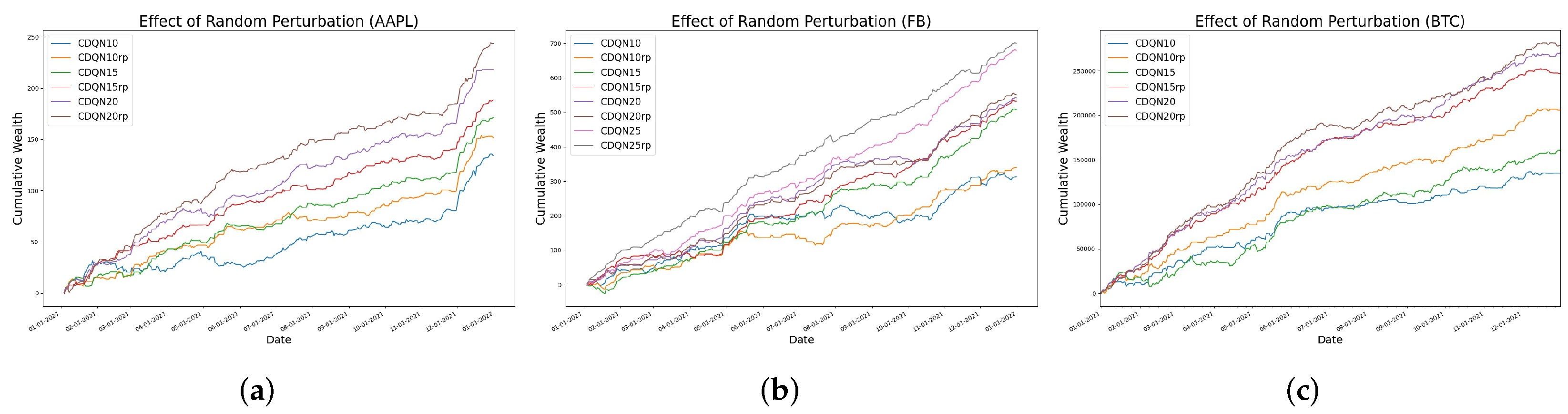
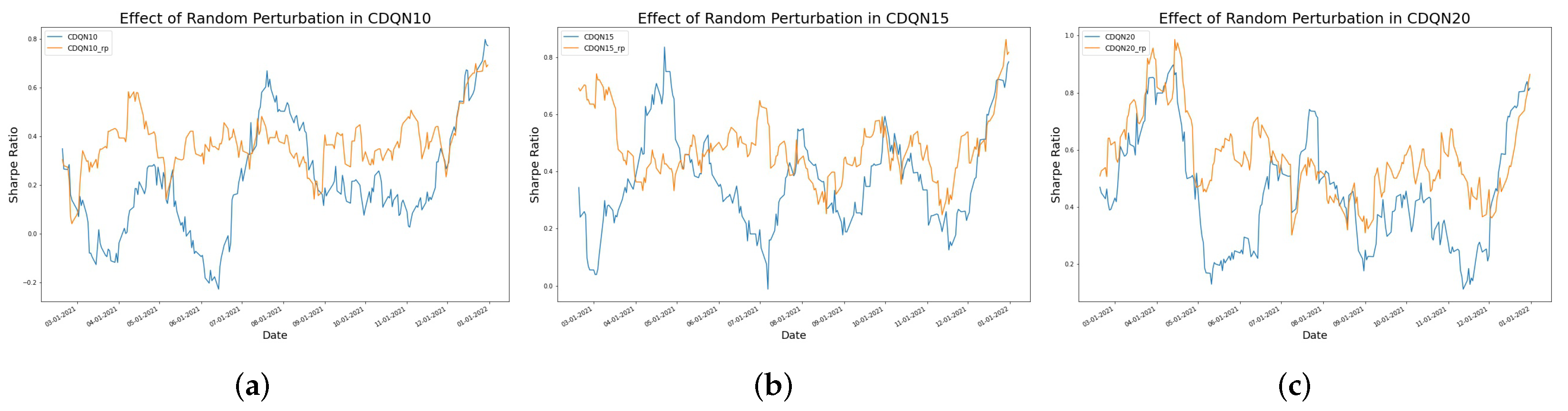
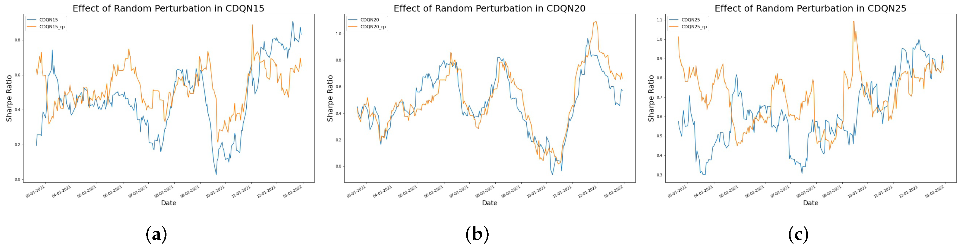
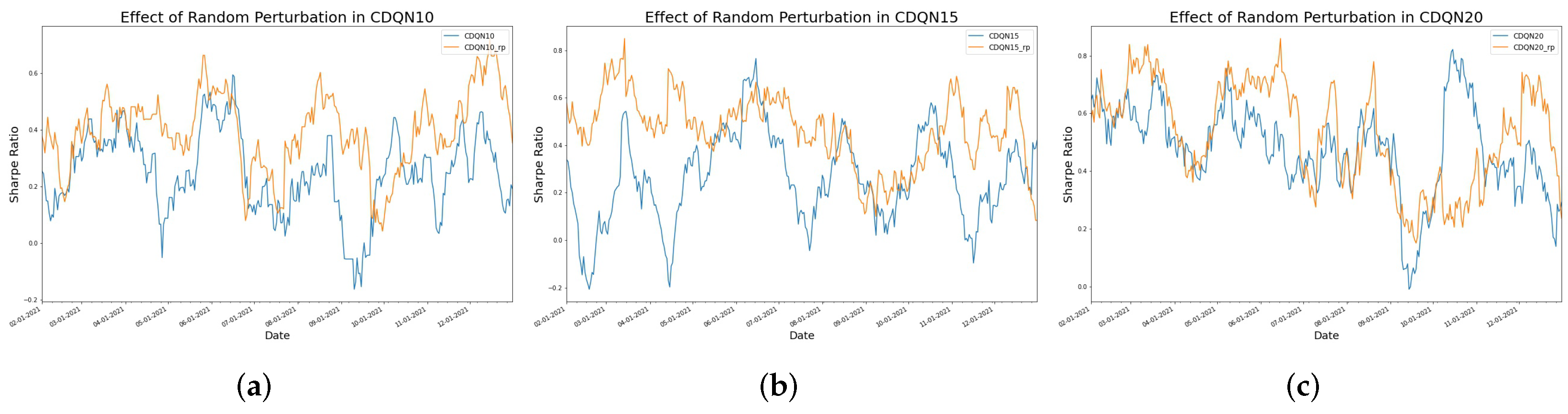
4.3. The Effect of Random Perturbation

The objective of this section is to compare the cumulative wealth and the Sharpe Ratio between the fixed step target network and random perturbation target network. As shown in Figure 6, for all three datasets, the random perturbation can improve the learning result in terms of the cumulative wealth, with detailed results summarized in

Table 2. Random Perturbation Effect on Cumulative Wealth for Different Datasets. The term “rp” in the parenthesis denotes the random perturbation technique.

Methods	AAPL	AAPL(rp)	FB	FB(rp)	BTC	BTC(rp)
CDQN10	134.13	151.77	313.58	340.12	134,939	205,791
CDQN15	171.20	188.49	508.15	531.92	160,155	247,023
CDQN20	218.26	243.83	541.91	551.52	269,967	278,092

. The figure shows the comparison between the cumulative wealth with or without the random perturbation target network. Clearly, for all cases, CDQN10, CDQN15, and CDQN20 (also CDQN25 for FB as the best scenario is $n=25$ for FB), the application of random perturbation can lead to higher cumulative wealth. Figure 7, Figure 8 and Figure 9 show that the random perturbation improves the Sharpe ratio as well, in all three cases, based on AAPL, FB, and Bitcoin respectively. Another advantage of the random perturbation is that the Sharpe ratio curve trained with random perturbation becomes more stable compared to that trained with the fixed step target network, especially for AAPL.

5. Discussion

Problems for which reinforcement learning (RL) is applicable usually involve a long-term reward that needs to be optimized and a sequence of decisions that needs to be learned. Quantitative trading is such a problem. In this section, we first recap the new RL method for quantitative trading that we have proposed in this work, and proceed to summarize our conclusions, limitations, and future research directions.

To recap, we first proposed the near-quadratic transaction cost model based on several key factors, such as market impact and bid/ask spread, which is often neglected by most papers work on quantitative trading. We then developed the convolutional deep Q-network (CDQN) with stacked prices strategy for trading. We addressed the connection between the convolution in deep learning and the technical analysis in traditional finance. Our analysis focused on selecting different number of historical prices, adding the convolutional and the pooling layers, and subsequently comparing these strategies to both the traditional buy and hold strategy and the modern LSTM stock prediction method.

We tested our methods by devloping RL trade strategies based on AAPL, FB, and BTC daily prices in 2021, and the results demonstrated that CDQN outperforms other commonly used trading strategies when transaction cost is included. In terms of the Sharpe ratio measurement, our CDQN method fluctuates a lot, indicating that our method cannot recognize all some sudden change points in the time series. This is especially pronounced for Bitcoin (BTC) as the cryptocurrency market can be especially volatile. To improve the trading stability and be more resistant to risk events has be one of our research foci. To solve the instability issue lying behind training a DQN, we have also designed the random perturbation method which randomized the step used to update the target network. This method can also be embedded on top of the double Q-networks without training a completely different network. We have demonstrated that our new random perturbation method can help the agent learn the environment faster than the typical fixed step DQN. In addition, for future studies, apart from the historical prices, other covariates such as socioeconomic variables, both domestic and international, will be added to capture the market information and to account for more exogeneous influences.

At present, one single asset is traded in our work—further research is needed to establish and to adjust the optimal portfolio weights. Furthermore, we will consider extending the action space from discrete to continuous to have better real-world applications. In this work, our focus was on methodology development, and we could run our algorithms on a personal computer in a span of hours. A related issue to be addressed, with a portfolio of equities and with continuous action space, will be the computational cost and efficiencies. Finally, in the future, we would also like to investigate different reward functions for our RL trading algorithms. Many reward functions in the quantitative trading field do not include risk measures, while in practice, an investor often prioritizes the risk over the net return.

References

1. Kober, J.; Bagnell, J.A.; Peters, J. Reinforcement learning in robotics: A survey. Int. J. Robot. Res. 2013, 32, 1238–1274. [Google Scholar] [CrossRef] [Green Version]
2. Kaiser, L.; Babaeizadeh, M.; Milos, P.; Osinski, B.; Campbell, R.H.; Czechowski, K.; Erhan, D.; Finn, C.; Kozakowski, P.; Levine, S.; et al. Model-based reinforcement learning for atari. arXiv 2019, arXiv:1903.00374. [Google Scholar]
3. Mosavi, A.; Faghan, Y.; Ghamisi, P.; Duan, P.; Ardabili, S.F.; Salwana, E.; Band, S.S. Comprehensive review of deep reinforcement learning methods and applications in economics. Mathematics 2020, 8, 1640. [Google Scholar] [CrossRef]
4. Collins, A.G.E. Reinforcement learning: Bringing together computation and cognition. Curr. Opin. Behav. Sci. 2019, 29, 63–68. [Google Scholar] [CrossRef]
5. Zhong, Y.; Wang, C.; Wang, L. Survival Augmented Patient Preference Incorporated Reinforcement Learning to Evaluate Tailoring Variables for Personalized Healthcare. Stats 2021, 4, 776–792. [Google Scholar] [CrossRef]
6. Sun, S.; Wang, R.; An, B. Reinforcement Learning for Quantitative Trading. arXiv 2021, arXiv:2109.13851. [Google Scholar]
7. Sutton, R.S.; Barto, A.G. Reinforcement Learning: An Introduction; MIT Press: Cambridge, MA, USA, 2018. [Google Scholar]
8. Moody, J.; Saffell, M. Reinforcement learning for trading. Adv. Neural Inf. Process. Syst. 1998, 11, 918–923. [Google Scholar]
9. Mnih, V.; Kavukcuoglu, K.; Silver, D.; Rusu, A.A.; Veness, J.; Bellemare, M.G.; Graves, A.; Riedmiller, M.; Fidjeland, A.K.; Ostrovski, G.; et al. Human-level control through deep reinforcement learning. Nature 2015, 518, 529–533. [Google Scholar] [CrossRef] [PubMed]
10. LeCun, Y.; Bengio, Y.; Hinton, G. Deep learning. Nature 2015, 521, 436–444. [Google Scholar] [CrossRef] [PubMed]
11. Edelen, R.; Evans, R.; Kadlec, G. Shedding light on “invisible” costs: Trading costs and mutual fund performance. Financ. Anal. J. 2013, 69, 33–44. [Google Scholar] [CrossRef]
12. Edelen, R.M.; Evans, R.B.; Kadlec, G.B. Scale Effects in Mutual Fund Performance: The Role of Trading Costs. 17 March 2007. Available online: https://ssrn.com/abstract=951367 (accessed on 1 May 2022). [CrossRef] [Green Version]
13. Scherer, B.; Martin, R.D. Modern Portfolio Optimization with NuOPTTM, S-PLUS®, and S+ BayesTM; Springer Science & Business Media: Berlin/Heidelberg, Germany, 2007. [Google Scholar]
14. Lecesne, L.; Roncoroni, A. Optimal allocation in the S&P 600 under size-driven illiquidity. In ESSEC Working Paper; Amundi Institute: Paris, France, 2019. [Google Scholar]
15. Chen, P.; Lezmi, E.; Roncalli, T.; Xu, J. A note on portfolio optimization with quadratic transaction costs. arXiv 2020, arXiv:2001.01612. [Google Scholar] [CrossRef]
16. Murphy, J.J. Technical Analysis of the Financial Markets: A Comprehensive Guide to Trading Methods and Applications; Penguin: New York, NY, USA, 1999. [Google Scholar]
17. Watkins, C.J.; Dayan, P. Q-learning. Mach. Learn. 1992, 8, 279–292. [Google Scholar] [CrossRef]
18. Spoerer, C.J.; Kietzmann, T.C.; Mehrer, J.; Charest, I.; Kriegeskorte, N. Recurrent neural networks can explain flexible trading of speed and accuracy in biological vision. PLoS Comput. Biol. 2020, 16, e1008215. [Google Scholar] [CrossRef] [PubMed]
19. Van Hasselt, H.; Guez, A.; Silver, D. Deep reinforcement learning with double q-learning. In Proceedings of the AAAI Conference on Artificial Intelligence, Phoenix, AZ, USA, 12–17 February 2016; Volume 30. [Google Scholar]
20. O’Shea, K.; Nash, R. An introduction to convolutional neural networks. arXiv 2015, arXiv:1511.08458. [Google Scholar]
Figure 1. Convolutional deep Q-network diagram for quantitative trading. (a) The left policy network with parameters θ shows the first pass with the current state S t = ( s t n + 1 , s t n + 2 , , s t ) as input to the network, and the network produces the Q values associated with short, neutral and long actions, respectively. (b) The right target network with parameters θ shows the second pass with the next state S t = ( s t n + 2 , s t n + 3 , , s t + 1 ) as input, and the network outputs the state-action paired values Q ( S t + 1 , A t + 1 ) associated with the next state. The maximum value among Q ( S t + 1 , A t + 1 ) s is used to calculate the target Q values associated with the current state via the Q-learning algorithm.
Stats 05 00033 g001
Figure 2. The proposed convolutional deep Q-network (CDQN) with random perturbation (rp), that is, CDQN-rp algorithm for quantitative trading. First we store the (current state, next state, action, reward) tuples into the replay memory. The reward is then calculated based on the transaction costs (TCs) that we have modeled. Next, a sample from the replay memory is used to train the CDQN. During the training process, we apply the rp technique to update the target network. The action selected during the learning is based on both exploration and exploitation with the exploration rate following exponential decay. For decision making, we, or rather the agent, would select the action with the highest Q value for a given state.
Stats 05 00033 g002
Figure 3. Different trading strategies for AAPL (Apple Inc.). (a) The left figure shows the cumulative wealth curves in 2021 using different trading algorithms including DQNn ( n { 1 , 5 , 10 , 15 } ), CDQNn ( n { 10 , 15 , 20 , 25 } ), Buy and Hold, and LSTM. (b) The right figure shows the Sharpe ratio curves in 2021 using DQN15, CDQNn ( n { 10 , 15 , 20 , 25 } ), Buy and Hold, and LSTM.
Stats 05 00033 g003
Figure 4. Different trading strategies for FB (Meta Platforms, Inc.). (a) The left figure shows the cumulative wealth curves in 2021 using different trading algorithms including DQNn ( n { 1 , 5 , 10 , 15 } ), CDQNn ( n { 10 , 15 , 20 , 25 , 30 , 35 } ), Buy and Hold, and LSTM. (b) The right figure shows the Sharpe ratio curves in 2021 using DQN15, CDQNn ( n { 10 , 15 , 20 , 25 , 30 , 35 } ), Buy and Hold, and LSTM.
Stats 05 00033 g004
Figure 5. Different trading strategies for BTC (Bitcoin). (a) The left figure shows the cumulative wealth curves in 2021 using different trading strategies including CDQNn ( n { 5 , 10 , 15 , 20 , 25 , 30 } ) and Buy and Hold. (b) The right figure shows the Sharpe ratio curves in 2021 using CDQNn ( n { 5 , 10 , 15 , 20 , 25 , 30 } ) and Buy and Hold.
Stats 05 00033 g005
Figure 6. The effect of random perturbation measured by cumulative wealth. (a) The left figure shows the comparison between the cumulative wealth curves with or without the random perturbation technique in CDQN10, CDQN15, and CDQN20 for AAPL. (b) The middle figure shows the comparison between the cumulative wealth curves with or without the random perturbation technique in CDQN10, CDQN15, CDQN20, and CDQN 25 for FB. (c) The right figure shows the comparison between the cumulative wealth curves with or without the random perturbation technique in CDQN10, CDQN15, and CDQN20 for BTC.
Stats 05 00033 g006
Figure 7. The effect of random perturbation measured by Sharpe ratio for AAPL. (a) The left figure shows the comparison between the Sharpe ratio curves with or without the random perturbation technique in CDQN10. (b) The middle figure shows the comparison between the Sharpe ratio curves with or without the random perturbation technique in CDQN15. (c) The right figure shows the comparison between the Sharpe ratio curves with or without the random perturbation technique in CDQN20.
Stats 05 00033 g007
Figure 8. The effect of random perturbation measured by Sharpe ratio for FB. (a) The left figure shows the comparison between the Sharpe ratio curves with or without the random perturbation technique in CDQN15. (b) The middle figure shows the comparison between the Sharpe ratio curves with or without the random perturbation technique in CDQN20. (c) The right figure shows the comparison between the Sharpe ratio curves with or without the random perturbation technique in CDQN25.
Stats 05 00033 g008
Figure 9. The effect of random perturbation measured by Sharpe ratio for BTC. (a) The left figure shows the comparison between the Sharpe ratio curves with or without the random perturbation technique in CDQN10. (b) The middle figure shows the comparison between the Sharpe ratio curves with or without the random perturbation technique in CDQN15. (c) The right figure shows the comparison between the Sharpe ratio curves with or without the random perturbation technique in CDQN20.
Stats 05 00033 g009