Partially Linear Generalized Single Index Models for Functional Data (PLGSIMF)

Abstract

Single-index models are potentially important tools for multivariate non-parametric regression analysis. They generalize linear regression models by replacing the linear combination ${\alpha }_0^{\top }X$ with a non-parametric component ${\eta }_0\left({\alpha }_0^{\top }X\right)$, where ${\eta }_0(·)$ is an unknown univariate link function. In this article, we generalize these models to have a functional component, replacing the generalized partially linear single index models ${\displaystyle {\eta }_0\left({\alpha }_0^{\top }X\right)+{\beta }_0^{\top }Z}$, where $\alpha$ is a vector in ${\mathrm{I}\mathrm{R}}^d$, ${\eta }_0(·)$ and ${\beta }_0(·)$ are unknown functions that are to be estimated. We propose estimates of the unknown parameter ${\alpha }_0$, the unknown functions ${\beta }_0(·)$ and ${\eta }_0(·)$ and establish their asymptotic distributions, and furthermore, a simulation study is carried out to evaluate the models and the effectiveness of the proposed estimation methodology.

1. Introduction

Generalized linear models are proposed by Nelder and Wedderburn [1], $g\left(\mu \left(X\right)\right)={\beta }^{\top }X$; for a detail review, we refer the readers to McCullagh and Nelder [2]; it consists of a random component and systematic component. GLMs assume the responses come from the exponential dispersion model family. They extend linear models to allow the relationship between the predictors and the function of the mean of continuous or discrete response through a canonical link function. These models encounter problems such as the canonical link function is sometimes unknown, the link between response and predictors can be complex as well as the plague of dimension reduction. To address these problems, several approaches have been developed. Hastie and Tibshirani [3] propose the GAMs models, in which the linear predictor depends linearly on smooth of predictor variables, one of the criticisms of these models is that they do not take into consideration the interactions between covariates. The manuscripts of Wood [4] and Dunn, Peter, Smyth, Gordon [5] are the latest references dealing with these two models.

The single index model had been employed to reduce the dimensionality of data, and avoid the “curse of dimensionality” while maintaining the advantages of non-parametric smoothing in multivariate regression cases over the last few decades, see for example the work of Lai et al. [6].

The single index ${\alpha }^{\top }X$ aggregates the influence of the observed values $X=(X_1,\dots ,X_d)$ of the explanatory variables into one number.

Examples of economic index include the following: a stock index, inflation index, cost-of-living index, and price index.

Furthermore, this idea had first been extended to the functional setting by Ferraty, Vieu et al. [7] for functional regression problems, which led to the functional single index regression model (FSIRM). The functional index acts as a filter permitting the extraction of the part of explaining the scalar response Y, and plays an important role in a such model.

The predictor is not generally linear, but is complex, which prompted Caroll et al. [8] to propose their model GPLSIM by applying the local-quasi-likelihood function and the kernel type of smoothing by approximating the function ${\eta }_0$ using local linear methods $g\left(\mu (X,Z)\right)={\eta }_0\left({\alpha }_0^{\top }X\right)+{\beta }_0^{\top }Z$. A GPLSIM was proposed by Chin-Shang Li et al. [9], in which the unknown smooth function of single index was approximated by a spline function that can be expressed as a linear combination of B-spline basis function considered as follows $g\left(\mu (X,Z)\right)={\beta }^{\top }X+\phi \left({\alpha }^{\top }Z\right)$ using a modified Fisher-scoring method. Moreover, Wang and Cao [10], have studied the GPLSIM model by applying the quasi-likelihood and polynomial spline smoothing $g\left(\mu (X,Z)\right)={\eta }_0\left({\alpha }_0^{\top }X\right)+{\beta }_0^{\top }Z$.

In recent years, the analysis of functional data has made considerable progress in several areas, including image processing, biomedical studies, environmental sciences, public health, etc. Several researchers have focused their efforts on studying this type of data. We mention the work of Aneiros-Pérez and Vieu [11], and for more details, we refer to the books of Horváth Kokoszka [12], Ferraty and Vieu [7], Aneiros-Pérez and Vieu [13], and Ramsay and Silverman [14]. Yu, Du and Zhang [15] have proposed the SIPFLM model combining the single-index model (SIM) and the FLM model by optimizing the sum of the least squares using the B-Spline basis $Y=g\left({\alpha }^{\top }X\right)+{\int }_T\beta \left(t\right)Z\left(t\right)dt$. Jiang Du et al. [16] proposed the GFPLM model using the functional principal component analysis $g\left(\mu (X,Z)\right)={\alpha }^{\top }X+{\int }_T\beta \left(t\right)Z\left(t\right)dt$. Rachdi, Alahiane, Ouassou and Vieu presented a book chapter on the generalization of the GPLSIM model in the Iwfos 2020 conference, see Rachdi et al. [17]. Our objective is to combine the GPLSIM with the SIPFLM and consider the following generalized partially functional single-index model called PLGSIMF using B-Spline expansion and the quasi-likelihood function ${\displaystyle g\left(\mu (X,Z)\right)={\eta }_0\left({\alpha }^{\top }X\right)+{\int }_0^1\beta \left(t\right)Z\left(t\right)dt}$ in order to remedy the interaction effects, the dimension scourge and to take into account the functional random variables.

The paper is organized as follows. In Section 1 and Section 2, we localize our model in the literature, and we present the Fisher-scoring update algorithm used to estimate our single-index vector, the parametric function and the slope function. In Section 3, we investigate an asymptotic study of the estimators presented in the paper. Numerical simulation in the Gaussian case as in the logistic case is presented in Section 4. The proofs of the results are developed in Section 6 and in the Appendix A for the different technical lemmas necessary to develop our asymptotic study both for the non-parametric function, for the single-index vector and for the slope function.

Let H be a separable Hilbert space, which is endowed with the scalar product $<·,·{>}_H$ and the norm $\left|\right|·{\left|\right|}_H$. Let Y be a scalar response variable and $(X,Z)\in {\mathrm{I}\mathrm{R}}^d\times H$ be the predictor vector where $X=(X_1,\dots ,X_d)$ and Z to be a functional random variable that is valued in H. For a fixed $(x,z)\in {\mathrm{I}\mathrm{R}}^d\times H$, we assume that the conditional density function of the response Y given $(X,Z)=(x,z)$ belongs to the following canonical exponential family:

$$f_{Y|X=x,Z=z}\left(y\right)=exp\left(y\xi (x,z)-B\left(\xi \right(x,z\left)\right)+C\left(y\right)\right),$$

(1)

where B and C are two known functions that are defined from $\mathrm{I}\mathrm{R}$ into $\mathrm{I}\mathrm{R}$, and $\xi :{\mathrm{I}\mathrm{R}}^d\times H⟶\mathrm{I}\mathrm{R}$ is the parameter in the generalized parametric linear model, which is linked to the dependent variable

$$\mu (x,z)=\mathbb{E}\left[Y|X=x,Z=z\right]=B^{\prime }\left(\xi (x,z)\right),$$

(2)

where $B^{\prime }$ denotes the first derivative of the function B. In what follows, we consider the function $g\left(\mu \right(x,z\left)\right)$ as a generalized single-index partially functional linear model:

$$g\left(\mu (x,z)\right)={\eta }_0\left({\alpha }^{\top }x\right)+{\int }_0^1\beta \left(t\right)z\left(t\right)dt,$$

(3)

where $\alpha =\left({\alpha }_1,{\alpha }_2,\dots ,{\alpha }_d\right)\in {\mathrm{I}\mathrm{R}}^d$ is the d-dimensional single-index coefficient vector, $\beta$ is the coefficient function in the functional component, and ${\eta }_0$ is the unknown single-index link function which will be assumed to be sufficiently smooth.

If the conditional variance $Var\left(Y\right|X=x,Z=z)={\sigma }^{2}V\left(\mu (x,z)\right)$, where V is an unknown positive function, then the estimation of the mean function $g\left(\mu \right)$ may be obtained by replacing the log-likelihood $f_{Y|X=x,Z=z}$ given by (1), by the quasi-likelihood $Q(u,v)$ given by

$$\frac{\partial Q(u,v)}{\partial u}=\frac{v-u}{{\sigma }^{2}V\left(u\right)},$$

for any real numbers u and v, which may be written as ${\displaystyle Q(u,v)={\int }_v^u\frac{v-t}{{\sigma }^{2}V\left(t\right)}\mathrm{d}t}$.

2. Estimation Methodology

Let ${\left(X_i,Y_i,Z_i\right)}_{i=1,\dots ,n}$ be a sequence of independent and identically distributed (i.i.d.) as $(X,Y,Z)$ and, for each $i=1,\dots ,n$,

$$g\left(\mu \left(X_i,Z_i\right)\right)={\eta }_0\left({\alpha }^{\top }{X}_i\right)+{\int }_0^1\beta \left(t\right)Z_i\left(t\right)dt.$$

(4)

We assume that the function ${\eta }_0$ is supported within the interval $[a,b]$ where $a=inf\left({\alpha }^{\top }X\right)$ and $b=sup\left({\alpha }^{\top }X\right)$.

We introduce a sequence of knots $\left(k_m\right)$ in the interval $[a,b]$, with J interior knots, such that $k_{-r+1}=\cdots =k_{-1}=k_0=a<k_1<\cdots <k_J=k_{J+1}=\cdots =k_{J+r}$, where $J:=J_n$ is a sequence of integers which increases with the sample size n. Now, let $N_n=J_n+r$ be the number of knots, ${\left(B_j\left(u\right)\right)}_{j=1,\dots ,N_n}$ be the B-spline basis functions of order r, and $h=(b-a)/(J_n+1)$ be the distance between the neighbors knots.

Let ${\mathcal{S}}_n$ be the space of polynomial splines on $[a,b]$ of order $r\ge 1$. By De Boor [18], we can approximate ${\eta }_0,$ assumed in $\mathcal{H}\left(p\right)$ (which will be defined in Section 3) by a function $\tilde{\eta }\in {\mathcal{S}}_n$. So, we can write $\tilde{\eta }\left(u\right)={\tilde{\gamma }}^{\top }B\left(u\right)$ where $B\left(u\right)$ is the spline basis and $\tilde{\gamma }\in {\mathrm{I}\mathrm{R}}^{N_n}$ is the spline coefficient vector.

We introduce a new knots sequence $0=t_0<t_1<\cdots <t_{k+1}=1$ of $[0,1]$. Then, there exists $N^{\prime }=k+r+1$ functions in the B-splines basis which are normalized and of order r, such that

$$\beta (·)\approx {\delta }^{\top }{B}_2(.)\mathrm{where}{B}_2(.)={\left(B_{21}(.),B_{22}(.),\dots ,B_{2N^{\prime }}(.)\right)}^{\top }\mathrm{and}\delta \in {\mathrm{I}\mathrm{R}}^{N^{\prime }}.$$

By setting

$$W=\left({\int }_0^{1}Z\left(t\right)B_{21}\left(t\right)dt,\dots ,{\int }_0^{1}Z\left(t\right)B_{2N^{\prime }}\left(t\right)dt\right),$$

(5)

and w and $W_i$ are defined accordingly to (5), the mean function estimator $\widehat{\mu }\left(x,z\right)$ is then given by the evaluation of the parameter $\theta ={\left({\alpha }^{\top },{\gamma }^{\top },{\delta }^{\top }\right)}^{\top }$ and by inverting the following equation $g\left(\widehat{\mu }\left(x,z\right)\right)={\widehat{\gamma }}^{\top }{B}_1\left({\widehat{\alpha }}^{\top }x\right)+{\widehat{\delta }}^{\top }w.$ Notice that the parameter $\theta ={\left({\alpha }^{\top },{\gamma }^{\top },{\delta }^{\top }\right)}^{\top }$ is determined by maximizing the following quasi-likelihood rule

$$\begin{array}{c}\hfill \widehat{\theta }={\left({\widehat{\alpha }}^{\top },{\widehat{\gamma }}^{\top },{\widehat{\delta }}^{\top }\right)}^{\top }=\underset{\theta =(\alpha ,\gamma ,\delta )\in {\mathrm{I}\mathrm{R}}^d\times {\mathrm{I}\mathrm{R}}^{N_n}\times {\mathrm{I}\mathrm{R}}^{N^{\prime }}}{argmax}l\left(\theta \right),\end{array}$$

where $l\left(\theta \right):=l(\alpha ,\gamma ,\delta )=\frac{1}{n}{\sum }_{i=1}^{n}Q\left(g^{-1}\left(m_i\right),Y_i\right)$, with

$$m\left(x,z\right)={\gamma }^{\top }{B}_1\left({\alpha }^{\top }x\right)+{\delta }^{\top }\omega ,$$

$$m_i:={\gamma }^{\top }{B}_1\left({\alpha }^{\top }{X}_i\right)+{\delta }^{\top }{W}_i\mathrm{and}{m}_{0i}={\gamma }_0^{\top }{B}_1\left(U_{0i}\right)+{\delta }_0^{\top }{W}_i,$$

where $U_{0i}={\alpha }_0^{\top }{X}_i$ with ${\alpha }_0$, ${\gamma }_0$, ${\delta }_0$, ${\eta }_0$, ${\beta }_0$ denoting the true values, respectively, of $\alpha$, $\gamma$, $\delta$, $\eta$ and $\beta$.

To overcome the constraint $\parallel \alpha \parallel =1$ and ${\alpha }_1>0$ of the d-dimensional index $\alpha$, we proceed by a re-parameterization, which is similar to Yu and Ruppert [19]

$$\alpha \left(\tau \right)={\left(\sqrt{1-{\parallel \tau \parallel }^2},{\tau }^{\top }\right)}^{\top }\mathrm{for}\tau \in {\mathrm{I}\mathrm{R}}^{d-1}.$$

The true value ${\tau }_0$ of $\tau$, must satisfy $∥{\tau }_0∥\le 1$. Then, we assume that $∥{\tau }_0∥<1$. The jacobian matrix of $\alpha :\tau \to \alpha \left(\tau \right)$ of dimension $d\times (d-1)$ is $J\left(\tau \right)$. Notice that $\tau$ is unconstrained and is one dimension lower than $\alpha$.

Finally, let

$$R\left(\tau \right)=\left(\begin{array}{cc}J\left(\tau \right)& 0\\ 0& I_{N^{\prime }\times N^{\prime }}\end{array}\right)$$

the jacobian matrix of ${\left(\alpha {\left(\tau \right)}^{\top },{\delta }^{\top }\right)}^{\top }$, which is of dimension $\left(d+N^{\prime }\right)\times \left(d+N^{\prime }-1\right)$. Let

$${\displaystyle (\tilde{\alpha },\tilde{\delta })=\underset{(\alpha ,\delta )\in {\mathrm{I}\mathrm{R}}^d\times {\mathrm{I}\mathrm{R}}^{N^{\prime }},\tau \in {\mathrm{I}\mathrm{R}}^{d-1}}{argmax}{\displaystyle \frac{1}{n}}\sum _{i=1}^{n}Q\left(g^{-1}\left\{\tilde{\eta }\left({\alpha }^{\top }\left(\tau \right)X_i\right)+{\delta }^{\top }{W}_i\right\},Y_i\right)\mathrm{and}{T}_i={\left(X_i^{\top },W_i^{\top }\right)}^{\top },}$$

Denote

$$\begin{array}{ccc}\hfill m_i& =& {\gamma }^{\top }{B}_1\left({\alpha }^{\top }{X}_i\right)+{\delta }^{\top }{W}_i,T_i={\left(X_i^{\top },W_i^{\top }\right)}^{\top },\hfill \\ \hfill m_{0i}& =& m_{0i}\left(X_i,W_i\right)={\gamma }_0^{\top }{B}_1\left({\alpha }_0^{\top }{X}_i\right)+{\delta }_0^{\top }{W}_i={\gamma }_0^{\top }{B}_1\left(U_{0i}\right)+{\delta }_0^{\top }{W}_i\mathrm{with}{U}_{0i}={\alpha }_0^{\top }{X}_i,\hfill \\ \hfill m_0\left(T\right)& =& {\gamma }_0^{\top }{B}_1\left({\alpha }_0^{\top }X\right)+{\delta }_0^{\top }W={\gamma }_0^{\top }{B}_1\left(U_0\right)+{\delta }_0^{\top }W\mathrm{with}{U}_0={\alpha }_0^{\top }X.\hfill \end{array}$$

and $(\tilde{\tau },\tilde{\delta })=\underset{\tau ,\delta }{argmax}\tilde{l}(\tau ,\delta )$ where $\tilde{l}(\tau ,\delta )=\frac{1}{n}{\sum }_{i=1}^{n}Q\left(g^{-1}\left\{\tilde{\eta }\left(\alpha {\left(\tau \right)}^{\top }{X}_i\right)+{\delta }^{\top }{W}_i\right\},Y_i\right)$. Note that ${\theta }_{\tau }={\left({\tau }^{\top },{\gamma }^{\top },{\delta }^{\top }\right)}^{\top }$ is a $(d-1)\times N_n\times N^{\prime }$-dimensional parameter, while $\theta$ is a $d\times N_n\times N^{\prime }$-dimensional one. Let

$${\rho }_l\left(m\right)=\frac{1}{{\sigma }^{2}V\left(g^{-1}\left(m\right)\right)}{\left[\frac{d}{dm}\left(g^{-1}\left(m\right)\right)\right]}^l$$

and denote

$$q_l(m,y)=\frac{{\partial }^l}{\partial m^l}Q\left(g^{-1}\left(m\right),y\right),\mathrm{for}l=1,2.$$

Then,

$$q_1(m,y)=\left(y-g^{-1}\left(m\right)\right){\rho }_1\left(m\right)\mathrm{and}{q}_2(m,y)=\left(y-g^{-1}\left(m\right)\right){\rho }_1^{\prime }\left(m\right)-{\rho }_2\left(m\right).$$

So, $l\left({\theta }_{\tau }\right)$ becomes

$$l\left({\theta }_{\tau }\right)=\frac{1}{n}\sum _{i=1}^{n}Q\left(g^{-1}\left\{{\gamma }^{\top }{B}_1\left({\alpha }^{\top }\left(\tau \right)X_i\right)+{\delta }^{\top }{W}_i\right\},Y_i\right)=\frac{1}{n}\sum _{i=1}^{n}Q\left(g^{-1}\left\{m_i\right\},Y_i\right)$$

The score vector is then

$$S\left({\theta }_{\tau }\right)=\frac{\partial l}{\partial {\theta }_{\tau }}\left({\theta }_{\tau }\right)=\frac{1}{n}\sum _{i=1}^n{q}_1\left(m_i,Y_i\right){\xi }_i(\tau ,\gamma ,\delta ),$$

where

$${\xi }_i(\tau ,\gamma ,\delta )=\left(\begin{array}{c}{\gamma }^{\top }{B}_1^{\prime }\left({\alpha }^{\top }\left(\tau \right)X_i\right)J^{\top }\left(\tau \right)X_i\\ B_1\left({\alpha }^{\top }\left(\tau \right)X_i\right)\\ W_i\end{array}\right).$$

The expectation of the Hessian matrix is

$$\begin{array}{ccc}\hfill H\left({\theta }_{\tau }\right)& =& \mathbb{E}\left[\frac{{\partial }^2}{\partial {\theta }_{\tau }^{\top }\partial {\theta }_{\tau }}S\left({\theta }_{\tau }\right)\right]\hfill \\ & =& -\frac{1}{n}\sum _{i=1}^n{\rho }_2\left(m_i\right){\xi }_i(\tau ,\gamma ,\delta ){\xi }_i^{\top }(\tau ,\gamma ,\delta ),\hfill \end{array}$$

The Fisher Scoring update equations ${\displaystyle {\theta }_{\tau }^{(k+1)}={\theta }_{\tau }^{\left(k\right)}-{\left[H\left({\theta }_{\tau }^{\left(k\right)}\right)\right]}^{-1}S\left({\theta }_{\tau }^{\left(k\right)}\right)}$, becomes

$$\begin{array}{ccc}\hfill {\theta }_{\tau }^{(k+1)}& =& {\theta }_{\tau }^{\left(k\right)}+{\left[\sum _{i=1}^n{\rho }_2\left(m_i^{\left(k\right)}\right){\xi }_i\left({\tau }^{\left(k\right)},{\gamma }^{\left(k\right)},{\delta }^{\left(k\right)}\right){\xi }_i^{\top }\left({\tau }^{\left(k\right)},{\gamma }^{\left(k\right)},{\delta }^{\left(k\right)}\right)\right]}^{-1}\hfill \\ & & \times \left[\sum _{i=1}^n\left(Y_i-{\mu }_i^{\left(k\right)}\right){\rho }_1\left(m_i^{\left(k\right)}\right){\xi }_i\left({\tau }^{\left(k\right)},{\gamma }^{\left(k\right)},{\delta }^{\left(k\right)}\right)\right],\hfill \end{array}$$

where $m_i^{\left(k\right)}={\gamma }^{\left(k\right)\top }{B}_1\left({\alpha }^{\left(k\right)\top }\left({\tau }^{\left(k\right)}\right)X_i\right)+{\delta }^{\left(k\right)\top }{W}_i$, for $1\le i\le n$ and ${\mu }_i^{\left(k\right)}=g^{-1}\left(m_i^{\left(k\right)}\right)$.

It follows that

$$\begin{array}{ccc}\hfill \widehat{\beta }\left(t\right)& =& {\widehat{\delta }}^{\top }{B}_2\left(t\right)={\delta }^{\left(k\right)\top }{B}_2\left(t\right),\widehat{\eta }\left(t\right)={\widehat{\gamma }}^{\top }{B}_1\left(t\right)={\gamma }^{\left(k\right)\top }{B}_1\left(t\right),\hfill \\ \hfill {\widehat{m}}_i& =& {\widehat{\gamma }}^{\top }{B}_1\left({\alpha }^{\top }\left(\widehat{\tau }\right)X_i\right)+{\widehat{\delta }}^{\top }{W}_i={\gamma }^{\left(k\right)\top }{B}_1\left({\alpha }^{\top }\left({\tau }^k\right)\right)X_i+{\delta }^{\left(k\right)\top }{W}_i,\hfill \end{array}$$

where ${\widehat{\mu }}_i=g^{-1}\left({\widehat{m}}_i\right)$, and $\widehat{\alpha }=\alpha \left({\tau }^{\left(k\right)}\right)$ is the estimator of the single-index coefficient vector of the PLGSIMF model.

3. Some Asymptotics

We present asymptotic properties of the estimators for the non-parametric components, the functional component, the single-index coefficient vector and the slope function of the PLGSIMF model. For this aim, we will need some assumptions.

3.1. Some Additional Notions and Assumptions

Let $\phi$, ${\phi }_1$ and ${\phi }_2$ be measurable functions on $[a,b]$. We define the empirical inner product ${〈{\phi }_1,{\phi }_2〉}_n$ and its corresponding norm ${\parallel \phi \parallel }_n$ as follows

$${\displaystyle {〈{\phi }_1,{\phi }_2〉}_n={\displaystyle \frac{1}{n}}\sum _{i=1}^n{\phi }_1\left(U_i\right){\phi }_2\left(U_i\right)\mathrm{and}{\parallel \phi \parallel }_n^2={\displaystyle \frac{1}{n}}\sum _{i=1}^n{\phi }^2\left(U_i\right)\mathrm{where}{U}_i={\alpha }^{\top }{X}_i.}$$

If $\phi$, ${\phi }_1$ and ${\phi }_2$ are $L^2$-integrable, we define the theoretical inner product and its corresponding norm as follows

$$〈{\phi }_1,{\phi }_2〉=\mathbb{E}\left[{\phi }_1\left(U\right){\phi }_2\left(U\right)\right]\mathrm{and}{\parallel \phi \parallel }_2^2=\mathbb{E}\left[{\phi }^2\left(U\right)\right]={\int }_a^b{\phi }^2\left(u\right)f\left(u\right)du.$$

Let $v\in {\mathbb{N}}^{*}$ and $e\in (0,1]$ such that $p=v+e>1.5$. We denote by $\mathcal{H}\left(p\right)$ the collection of functions g, which are defined on $[a,b]$ whose v-th order derivative, $g^{\left(v\right)}$, exists and satisfies the following e-th order Lipschitz condition

$$\left|g^{\left(v\right)}\left(m^{\prime }\right)-g^{\left(v\right)}\left(m\right)\right|\le C{\left|m^{\prime }-m\right|}^e,\mathrm{for}\mathrm{all}a\le m,m^{\prime }\le b.$$

Let $\epsilon =Y-g^{-1}\left(m_0\left(T\right)\right)$ where $T={\left(X^{\top },W^{\top }\right)}^{\top }$.

(C1) The single-index link function ${\eta }_0\in \mathcal{H}\left(p\right)$, where $\mathcal{H}\left(p\right)$ is defined as above.

(C2) For all $m\in \mathrm{I}\mathrm{R}$ and for all y in the range of the response variable Y, the function $q_2(m,y)$ is strictly negative, and for $k=1,2$, there exist some positive constants $c_q$ and $C_q$ such that $c_q<\left|q_2^k(m,y)\right|<C_q.$

(C3) The marginal density function of ${\alpha }^{\top }X$ is continuous and bounded away from zero and is infinite on its support $[a,b]$. The v-th order partial derivatives of the joint density function of X satisfy the Lipschitz condition of order $\alpha$ ($\alpha \in (0,1]$).

(C4) For any vector $\tau$, there exist positive constants $c_{\tau }$ and $C_{\tau }$, such that

$$c_{\tau }{I}_{t\times t}\le \mathbb{E}\left[\left(\begin{array}{c}1\hfill \\ T\hfill \end{array}\right){\left(\begin{array}{c}1\hfill \\ T\hfill \end{array}\right)}^{\top }|{\alpha }^{\top }\left(\tau \right)X={\alpha }^{\top }\left(\tau \right)x\right]\le C_{\tau }{I}_{t\times t},$$

where $t=1+N_n+N^{\prime }$ and $T={\left(X^{\top },W^{\top }\right)}^{\top }$.

(C5) The number of knots $N_n$ satisfy $n^{\frac{1}{2(p+1)}}\ll N_n\ll n^{\frac{1}{8}}$, for $p>3$.

(C6) The fourth order moment of the random variable Z is finite, i.e., ${\mathbb{E}\parallel Z(.)\parallel }^4\le C$, where C denotes a generic positive constant.

(C7) The covariance function $K(t,s)=Cov\left(Z\right(t),Z(s\left)\right)$ is positive definite.

(C8) The slope function $\beta$ is a r-th order continuously differentiable function, i.e., $\beta \in {\mathcal{C}}^r\left([0,1]\right).$

(C9) For some finite positive constants $C_{\rho }$, $C_{\rho }^{*}$ and $M_0$

$$\left|{\rho }_1\left(m_0\right)\right|\le C_{\rho }\mathrm{and}\left|{\rho }_1\left(m\right)-{\rho }_1\left(m_0\right)\right|\le C_{\rho }^{*}\left|m-m_0\right|\mathrm{for}\mathrm{all}\left|m-m_0\right|\le M_0.$$

(C10) For some finite positive constants $C_g$, $C_g^{*}$ and $M_1$, the link function g, in the model (3), satisfies: ${\displaystyle \left|\frac{d}{dm}g\left(m\right){|}_{m=m_0}\right|\le C_g}$ and, for all $\left|m-m_0\right|\le M_1$,

$$\left|\frac{d}{dm}{g}^{-1}\left(m\right)-\frac{d}{dm}{g}^{-1}\left(m\right){|}_{m=m_0}\right|\le C_g^{*}\left|m-m_0\right|.$$

(C11) It exists a positive constant $C_0$, such that $\mathbb{E}\left({ϵ}^2\right|U_{\tau ,0})\le C_0,\mathrm{where}ϵ=Y-g^{-1}\left(m_0\left(T\right)\right)$.

3.2. Estimators Consistencies

Next we formulate several assertions on the considered estimators.

3.3. Estimation of the Nonparametric Component

The following theorem states the convergence, with rates, of the estimator $\widehat{\eta }.$

Theorem 1.

Under assumptions $\left(C_6\right)-\left(C_8\right)$, we have

$${∥\widehat{\eta }-{\eta }_0∥}_2={\mathcal{O}}_{\mathrm{I}\mathrm{P}}\left\{\sqrt{N_n}\left(\frac{1}{\sqrt{n}h}+h^p\right)\right\}\mathrm{and}{∥\widehat{\eta }-{\eta }_0∥}_n={\mathcal{O}}_{\mathrm{I}\mathrm{P}}\left\{\sqrt{N_n}\left(\frac{1}{\sqrt{n}h}+h^p\right)\right\},$$

where ${\mathcal{O}}_{\mathrm{I}\mathrm{P}}$ denotes a “grand O of Landau” in probability.

Proof of Theorem 1.

The proof of the previous theorem is given in the Appendix A. □

3.4. Estimation of the Slope Function

Theorem 2.

Under assumptions $\left(C_1\right)-\left(C_8\right)$, and $k\sim n^{1/(2r+1)}$, we have

$$\parallel \widehat{\beta }(·)-{\beta }_0{(·)\parallel }^2={\mathcal{O}}_{\mathrm{I}\mathrm{P}}\left(N_n^2{\left(h^p+\frac{1}{\sqrt{nh}}\right)}^2\right)+{\mathcal{O}}_{\mathrm{I}\mathrm{P}}\left(n^{-2r/(2r+1)}\right).$$

Proof of Theorem 2.

The proof of the previous theorem is given in the Appendix A. □

3.5. Estimation of the Parametric Components

The next theorem shows that the maximum quasi-likelihood estimator is root-n consistent and is asymptotically normal, although the convergence rate of the non-parametric component $\widehat{\eta }$ is slower than root-n. Before enouncing the theorem, let us denote

$$\begin{array}{ccc}\hfill {\rm Y}\left(u_{\tau ,0}\right)=\frac{\mathbb{E}\left[X{\rho }_2\left(m_0\left(T\right)\right)|U_{\tau ,0}=u_{\tau ,0}\right]}{\mathbb{E}\left[{\rho }_2\left(m_0\left(T\right)\right)|U_{\tau ,0}=u_{\tau ,0}\right]}& ,& \Gamma \left(u_{\tau ,0}\right)=\frac{\mathbb{E}\left[W{\rho }_2\left(m_0\left(T\right)\right)|U_{\tau ,0}=u_{\tau ,0}\right]}{\mathbb{E}\left[{\rho }_2\left(m_0\left(T\right)\right)|U_{\tau ,0}=u_{\tau ,0}\right]},\hfill \\ \hfill \Phi \left(x\right)=\Phi \left(U_{\tau ,0},x\right)=x-{\rm Y}\left(u_{\tau ,0}\right)& \mathrm{and}& \Psi \left(w\right)=\Psi \left(U_{\tau ,0},w\right)=w-\Gamma \left(u_{\tau ,0}\right).\hfill \end{array}$$

Theorem 3.

Under assumptions $\left(C_1\right)-\left(C_{11}\right)$, the constrained quasi-likelihood estimators $\widehat{\alpha }$ and $\widehat{\delta }$ with $\parallel \widehat{\alpha }{\parallel }_d=1$ are jointly asymptotically normally distributed, i.e.,

$$\sqrt{n}\left(\begin{array}{c}\widehat{\alpha }-{\alpha }_0\\ \widehat{\delta }-{\delta }_0\end{array}\right)\stackrel{\mathcal{D}}{⟶}\mathcal{N}\left(0,R\left({\tau }_0\right)D^{-1}{R}^{\top }\left({\tau }_0\right)\right),$$

where $\stackrel{\mathcal{D}}{\to }$ denotes the convergence in distribution, and

$$D=\mathbb{E}\left[{\rho }_2\left(m_0\left(T\right)\right)\left(\begin{array}{c}{\eta }_0^{\prime }\left(U_{\tau ,0}\right)J^{\top }\left({\tau }_0\right)\Phi \left(X\right)\\ \Psi \left(W\right)\end{array}\right){\left(\begin{array}{c}{\eta }_0^{\prime }\left(U_{\tau ,0}\right)J^{\top }\left({\tau }_0\right)\Phi \left(X\right)\\ \Psi \left(W\right)\end{array}\right)}^{\top }\right],$$

and

$$R\left(\tau \right)=\left(\begin{array}{cc}J\left(\tau \right)& 0\\ 0& I_{N^{\prime }\times N^{\prime }}\end{array}\right).$$

Proof of Theorem 3.

The proof of the previous theorem is given in the Appendix A. □

Comments on the Assumptions

The smoothness condition in (C1) describes that the single-index function ${\eta }_0(·)$ can be approximated by functions in the B-spline space with a normalized basis. On the other hand, the condition (C2) ensures the uniqueness of the solution, where the condition (C3) is a smoothness condition on the joint and marginal density functions of ${\alpha }^{\top }X$ and X. The condition (C5) allows to obtain the rate of growth of the dimension of the spline spaces relative to the sample size. Conditions (C6) and(C7) are required for covariates function Z, and (C8) is a smoothness condition for slope function. Conditions, (C4) and (C9)–(C11) are technical lemmas that will be used to prove the cited theorems in this article.

Then, in this paper, we introduce a new generalized functional partially linear single-index model based on a combination of polynomial smoothing. The asymptotic properties of the resulting estimators under certain regularity asymptions are established for this model and hence the non-parametric component $\eta$ and the slope function $\beta$ are evaluated by the B-spline functions. Finally, we give some simulations to illustrate our results.

4. A Numerical Study

We conduct a simulation study in order to show our results’ effectiveness. We will treat two main cases of link functions: the identity and the logit link functions.

Recall that if the density of Y given $X=x$ and $Z=z$ is

$$f_{Y|X=x,Z=z}\left(y\right)=exp\left(y\xi (x,z)-B\left(\xi \right(x,z\left)\right)+C\left(y\right)\right),$$

then the link fuction

$$g\left(\mu (x,z)\right)=\mathbb{E}\left[Y|X=x,Z=z\right]=B^{\prime }\left(\xi (x,z)\right)\mathrm{and}V\left(\mu (x,z)\right)=\frac{B^{\prime \prime }\left(\xi (x,z)\right)}{{\sigma }^2}.$$

4.1. Case 1: Identity Link Function

We consider the case where the link function is the identity and the model

$$Y_i=sin\left\{\frac{\pi \left({\alpha }^{\top }{X}_i-A\right)}{B-A}\right\}+{\int }_0^1\beta \left(t\right)Z_i\left(t\right)dt+{\epsilon }_i\mathrm{for}i=1,\dots ,n.$$

(6)

The responses $Y_i$ are simulated according to the Equation (6), $X_i$ are taken uniformly over the interval $[-0.5,0.5]$, whereas the errors are normally distributed with mean 0 and variance $0.01$, ${\epsilon }_i\sim \mathcal{N}(0,0.01)$. Moreover, we take the following coefficients

$$\alpha =\frac{1}{\sqrt{3}}{(1,1,1)}^{\top },A=\frac{\sqrt{3}}{2}-\frac{1.645}{\sqrt{12}}\mathrm{and}B=\frac{\sqrt{3}}{2}+\frac{1.645}{\sqrt{12}}.$$

The function $\beta (·)$ and $Z_i(·)$ are given by

$${\displaystyle \beta \left(t\right)=\sqrt{2}sin\left(\frac{\pi t}{2}\right)+3\sqrt{2}sin\left(\frac{3\pi t}{2}\right)\mathrm{and}{Z}_i\left(t\right)=\sum _{j=1}^{50}{\xi }_j{v}_j\left(t\right)}$$

where $v_j\left(t\right)=\sqrt{2}sin\left((j-0.5)\pi t\right)$, ${\xi }_j=\mathcal{N}\left(0,{\lambda }_j\right)$ and ${\lambda }_j={\left((j-0.5)\pi \right)}^{-2}$.

The knots are selected according to the formula $C{n}^{\frac{1}{2r}}log\left(n\right)$ where $C\in [0.3,1]$ (Like in Wang and Cao [10]). We chose $C=0.6$ and we made 300 replications with samples of sizes $n=500$ and $n=1000$.

Computations of the bias, the standard deviation (SD) and the Mean Squared Error (MSE) with respect to (i) the parameter $\tau$, (ii) the parameter $\gamma$ and (iii) the parameter $\delta$ are summarized, for $n=500$ (respectively, $n=1000$), in the following

Table 1. Bias, SD and MSE according to the parameter $\tau$ for PLGSIMF with the identity link function and $n=500$.

	${\mathit{\tau }}_1$	${\mathit{\tau }}_2$
Bias	0.004	−0.0009
SD	0.0031	0.0025
MSE	2.6565 × 10${}^{-5}$	7.1819 × 10${}^{-6}$

,

Table 2. Bias, SD and MSE evolutions with respect to the parameter $\gamma$ variation for PLGSIMF with the identity link function and $n=500$.

	${\mathit{\gamma }}_1$	${\mathit{\gamma }}_2$	${\mathit{\gamma }}_3$	${\mathit{\gamma }}_4$	${\mathit{\gamma }}_5$	${\mathit{\gamma }}_6$	${\mathit{\gamma }}_7$	${\mathit{\gamma }}_8$	${\mathit{\gamma }}_9$
Bias	−0.0256	−0.0575	0.0526	0.1230	0.0471	−0.0015	−0.0148	0.0241	0.0005
SD	0.1834	0.2430	0.3037	0.3621	0.2049	0.3756	0.3101	0.2281	0.1710
MSE	0.0343	0.0624	0.0950	0.1463	0.0442	0.1411	0.0964	0.0526	0.0292

and

Table 3. Bias, SD and MSE evolutions with respect to the parameter $\delta$ variation for PLGSIMF with the identity link function and $n=500$.

	${\mathit{\delta }}_1$	${\mathit{\delta }}_2$	${\mathit{\delta }}_3$	${\mathit{\delta }}_4$	${\mathit{\delta }}_5$	${\mathit{\delta }}_6$	${\mathit{\delta }}_7$
Bias	−0.3444	−0.5969	−0.2527	0.0696	0.1093	0.0746	0.2909
SD	0.9457	0.5569	0.2565	0.0916	0.1059	0.1150	0.1669
MSE	1.0131	0.6664	0.1296	0.0132	0.0231	0.0188	0.1125

(respectively, in the

Table 4. Bias, SD and MSE according to the parameter $\tau$ for PLGSIMF with the identity link function and $n=1000$.

	${\mathit{\tau }}_1$	${\mathit{\tau }}_2$
Bias	0.0054	0.0021
SD	0.0023	0.0021
MSE	3.5152 × 10${}^{-5}$	9.5050 × 10${}^{-6}$

,

Table 5. Bias, SD and MSE evolutions with respect to the parameter $\gamma$ variation for PLGSIMF with the identity link function and $n=1000$.

	${\mathit{\gamma }}_1$	${\mathit{\gamma }}_2$	${\mathit{\gamma }}_3$	${\mathit{\gamma }}_4$	${\mathit{\gamma }}_5$	${\mathit{\gamma }}_6$	${\mathit{\gamma }}_7$	${\mathit{\gamma }}_8$	${\mathit{\gamma }}_9$
Bias	−0.0969	−0.2220	−0.1260	−0.0815	−0.0806	−0.0135	0.2509	0.2234	0.1636
SD	0.1583	0.2194	0.2478	0.3041	0.2098	0.3092	0.2509	0.2234	0.1636
MSE	0.0344	0.0974	0.0773	0.0991	0.0505	0.0958	0.1259	0.0998	0.0535

and

Table 6. Bias, SD and MSE evolutions with respect to the parameter $\delta$ variation for PLGSIMF with the identity link function and $n=1000$.

	${\mathit{\delta }}_1$	${\mathit{\delta }}_2$	${\mathit{\delta }}_3$	${\mathit{\delta }}_4$	${\mathit{\delta }}_5$	${\mathit{\delta }}_6$	${\mathit{\delta }}_7$
Bias	−0.2189	0.0665	−0.0113	−0.0025	−0.0171	−0.0006	−0.0231
SD	1.1558	0.3477	0.1447	0.0644	0.0712	0.0716	0.1296
MSE	1.3839	0.1253	0.0210	0.0041	0.0053	0.0051	0.0173

).

4.2. Case 2: Logit Link Function

By taking a logit link function, data are generated from the model

$$\mathrm{logit}\left\{P[Y_i=1|X_i,Z_i]\right\}=sin\left\{\frac{\pi \left({\alpha }^{\top }{X}_i-A\right)}{B-A}\right\}+{\int }_0^1\beta \left(t\right)Z_i\left(t\right)dt+{\epsilon }_i,i=1,\dots ,n.$$

for which we have kept the same parameters and the variables as for the identity link function. Then, similarly to the identity link function case, computations of the bias, SD and the MSE with respect to the parameters $\tau$, $\gamma$ and then $\delta$ are summarized, for $n=500$ (respectively, $n=1000$), in the

Table 7. Bias, SD and MSE evolutions with respect to the parameter $\tau$ variation for PLGSIMF with the logit link function and $n=500$.

	${\mathit{\tau }}_1$	${\mathit{\tau }}_2$
Bias	−0.0094	0.0059
SD	0.0102	0.0107
MSE	0.0002	0.0001

,

Table 8. Bias, SD and MSE evolutions with respect to the parameter $\gamma$ variation for PLGSIMF with the logit link function and $n=500$.

	${\mathit{\gamma }}_1$	${\mathit{\gamma }}_2$	${\mathit{\gamma }}_3$	${\mathit{\gamma }}_4$	${\mathit{\gamma }}_5$	${\mathit{\gamma }}_6$	${\mathit{\gamma }}_7$	${\mathit{\gamma }}_8$	${\mathit{\gamma }}_9$
Bias	0.6075	−0.1033	0.2749	0.1901	0.1506	0.1697	0.6662	0.5948	0.4662
SD	0.2720	0.1529	0.1832	0.1055	0.0850	0.1266	0.4510	0.3224	0.4455
MSE	0.4431	0.0340	0.1092	0.0473	0.0299	0.0448	0.6472	0.4577	0.4159

and

Table 9. Bias, SD and MSE evolutions with respect to the parameter $\delta$ variation for PLGSIMF with the logit link function and $n=500$.

	${\mathit{\delta }}_1$	${\mathit{\delta }}_2$	${\mathit{\delta }}_3$	${\mathit{\delta }}_4$	${\mathit{\delta }}_5$	${\mathit{\delta }}_6$	${\mathit{\delta }}_7$
Bias	−0.2977	0.7625	−0.3420	−0.2347	−0.0243	0.1246	0.0325
SD	0.9025	0.2310	0.5342	0.2008	0.2160	0.2149	0.3286
MSE	0.9031	0.6348	0.4024	0.0954	0.0472	0.0617	0.1090

(respectively, in the

Table 10. Bias, SD and MSE evolutions with respect to the parameter $\tau$ variation for PLGSIMF with the logit link function and $n=1000$.

	${\mathit{\tau }}_1$	${\mathit{\tau }}_2$
Bias	0.0054	0.0021
SD	0.0023	0.0021
MSE	3.5152 × 10${}^{-5}$	9.5050 × 10${}^{-6}$

,

Table 11. Bias, SD and MSE evolutions with respect to the parameter $\gamma$ variation for PLGSIMF with the logit link function and $n=1000$.

	${\mathit{\gamma }}_1$	${\mathit{\gamma }}_2$	${\mathit{\gamma }}_3$	${\mathit{\gamma }}_4$	${\mathit{\gamma }}_5$	${\mathit{\gamma }}_6$	${\mathit{\gamma }}_7$	${\mathit{\gamma }}_8$	${\mathit{\gamma }}_9$
Bias	−0.0969	−0.2220	−0.1260	−0.0815	−0.0806	−0.0135	0.2509	0.2234	0.1636
SD	0.1583	0.2194	0.2478	0.3041	0.2098	0.3092	0.2509	0.2234	0.1636
MSE	0.0344	0.0974	0.0773	0.0991	0.0505	0.0958	0.1259	0.0998	0.0535

and

Table 12. Bias, SD and MSE evolutions with respect to the parameter $\delta$ variation for PLGSIMF with the logit link function and $n=1000$.

	${\mathit{\delta }}_1$	${\mathit{\delta }}_2$	${\mathit{\delta }}_3$	${\mathit{\delta }}_4$	${\mathit{\delta }}_5$	${\mathit{\delta }}_6$	${\mathit{\delta }}_7$
Bias	−0.2189	0.0665	−0.0113	−0.0025	−0.0171	−0.0006	−0.0231
SD	1.1558	0.3477	0.1447	0.0644	0.0712	0.0716	0.1296
MSE	1.3839	0.1253	0.0210	0.0041	0.0053	0.0051	0.0173

).

It is obviously seen that the quality of the estimators are illustrated via simulations. The method performs quite well. The Bias, SD and MSE are reasonably small in general. The parametric and nonparametric components, the single-index and also the slope function are computed by the procedure given in this paper.

Both tables correspondingly indicate the consistency of $\widehat{\alpha }$ and $\widehat{\delta }$ as the bias, SD and MSE decrease as the sample size increasing. The knots selection with formula $C{n}^{\frac{1}{2r}}log\left(n\right)$ by using $C\in [0.3,1]$ like in Li Wang and Guanqun CAO [10], we have chosen $C=0.6$.

We developed our algorithm in both cases: the identity link function and the logistic link function. Simulations show that the PLGSIMF algorithm works well in both cases.

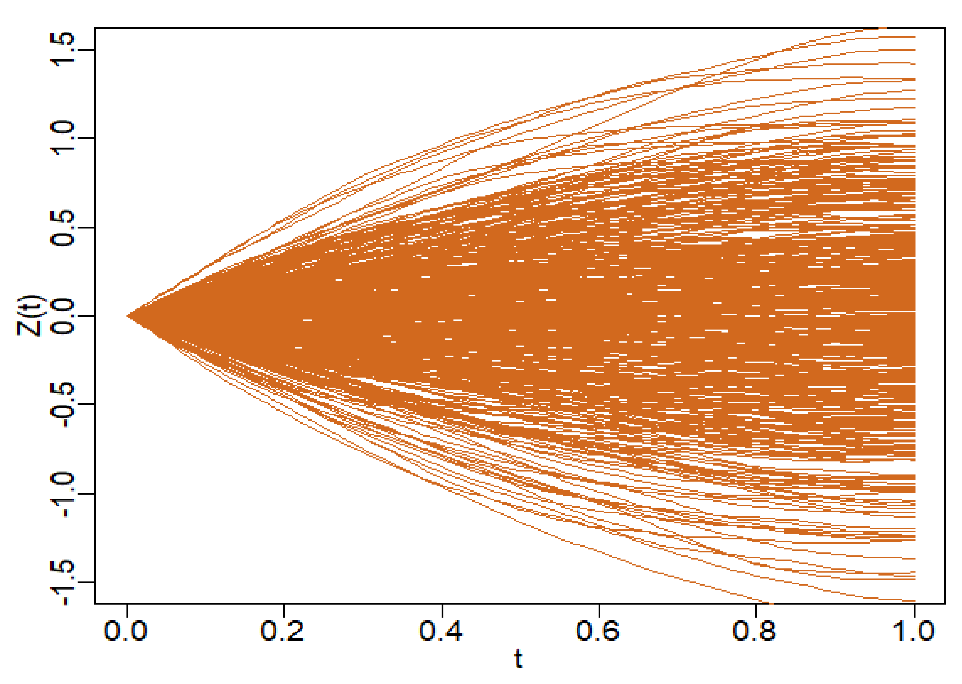
In the figure below (Figure 1), we illustrate 500 realizations of the functional random variable Z.

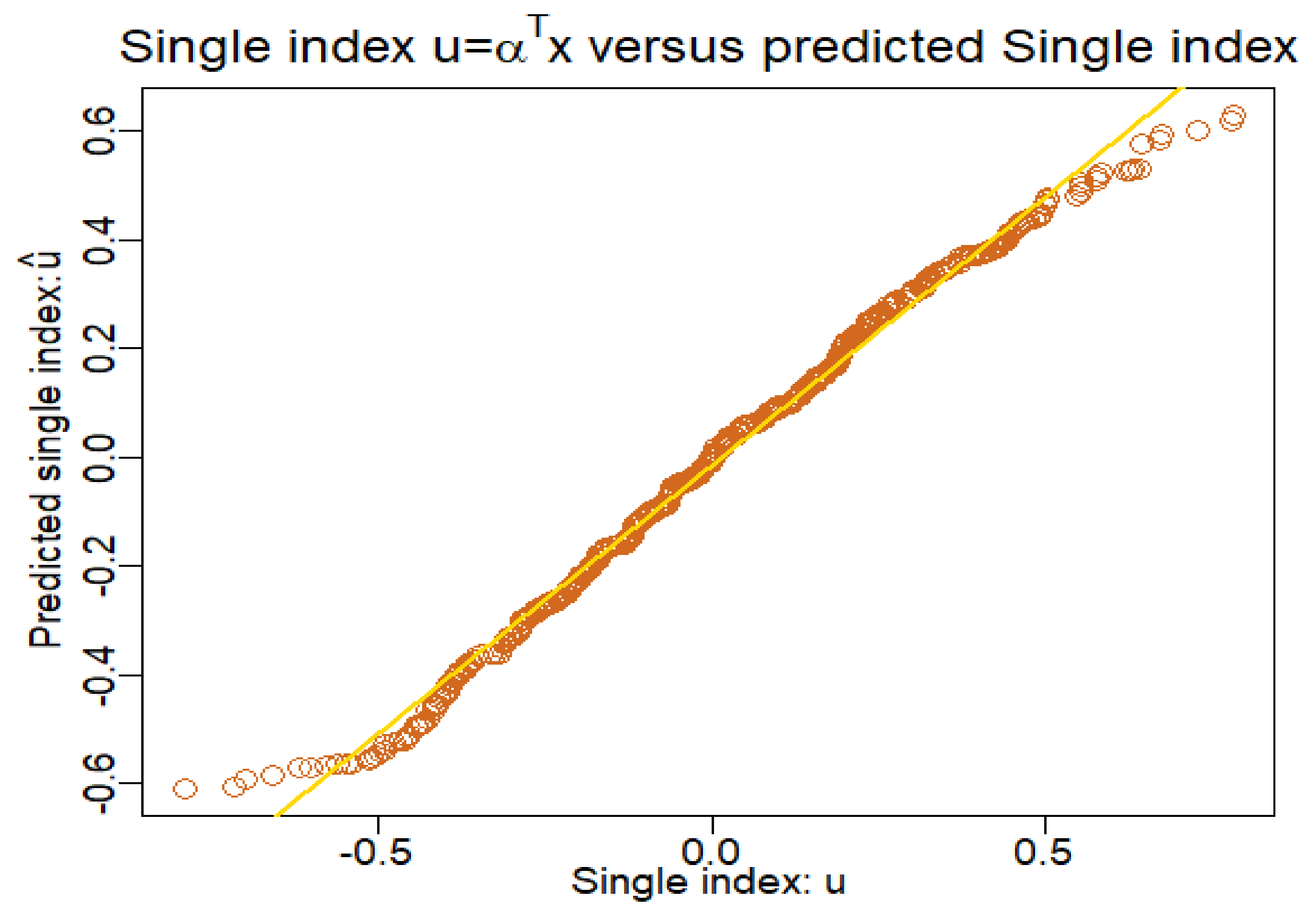
In the following figure (Figure 2), we observe the almost linearity of the single-index $u={\alpha }^{\top }\left(\tau \right)X$ and its estimate $\widehat{u}={\widehat{\alpha }}^{\top }\left(\widehat{\tau }\right)X.$

In the figure below (Figure 3), we plot the slope function $\beta (.)$ and its estimator $\widehat{\beta }(.)$

Our model approximates well the slope function $\beta (.)$.

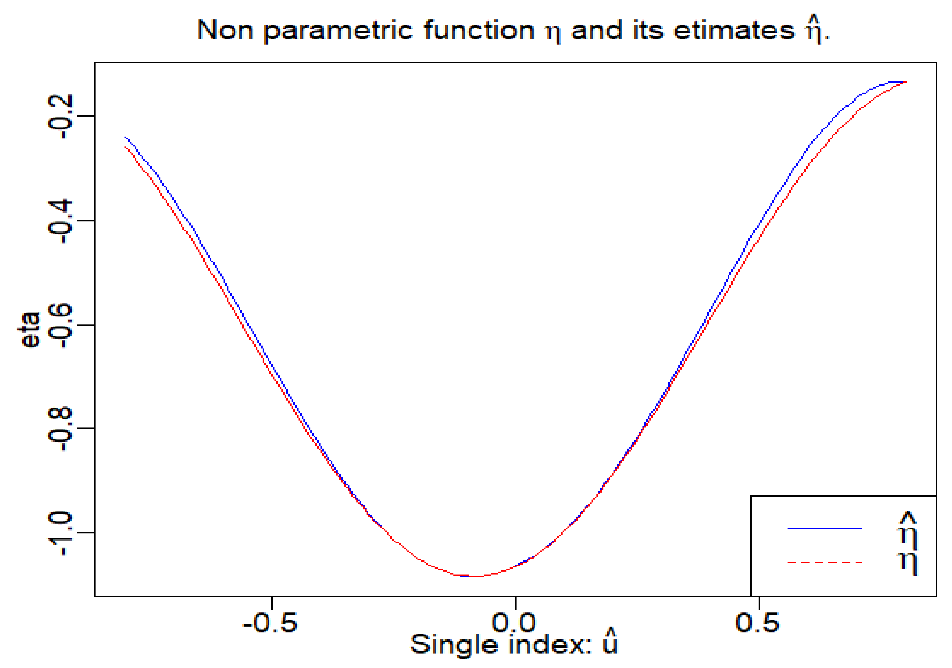
The following figure (Figure 4) shows us the comparison between the non-parametric function $\eta (.)$ and its estimator $\widehat{\eta }(.).$

We consider that our model approximated to the best the non-parametric function $\eta (.).$

To study the performance of our estimation for non-parametric function $\eta (.)$ and slope function, respectively, we will use the square root of average square errors criterion (RASE, see Peng et al. [20]):

$${\displaystyle {\mathrm{RASE}}_1={\left(\frac{1}{n}\sum _{i=1}^n{\left(\widehat{\eta }\left(u_i\right)-\eta \left(u_i\right)\right)}^2\right)}^{1/2}}$$

$${\displaystyle {\mathrm{RASE}}_2={\left(\frac{1}{n}\sum _{i=1}^n{\left(\widehat{\beta }\left(t_i\right)-\beta \left(t_i\right)\right)}^2\right)}^{1/2}}$$

The following tables (Table 13 amd Table 14) summarize the sample means, medians and variances of the RASE${}_i$ ($i=1,2$) with different sample sizes in the Gaussian case.

For the case $n=500$, we get

Table 13. The RASE criterion with the non-parametric function $\eta (.)$ and slope function $\beta (.)$ for the case $n=500$.

Gaussian Cases	Mean	Median	Var
RASE${}_1$	0.039	0.038	0.003
RASE${}_2$	0.123	0.122	0.020

Table 13. The RASE criterion with the non-parametric function $\eta (.)$ and slope function $\beta (.)$ for the case $n=500$.

Gaussian Cases	Mean	Median	Var
RASE${}_1$	0.039	0.038	0.003
RASE${}_2$	0.123	0.122	0.020

For the case $n=1000$, we get

Table 14. The RASE criterion with the non-parametric function $\eta (.)$ and slope function $\beta (.)$ for the case $n=1000$.

Gaussian Cases	Mean	Median	Var
RASE${}_1$	0.016	0.016	0.001
RASE${}_2$	0.027	0.125	0.006

Table 14. The RASE criterion with the non-parametric function $\eta (.)$ and slope function $\beta (.)$ for the case $n=1000$.

Gaussian Cases	Mean	Median	Var
RASE${}_1$	0.016	0.016	0.001
RASE${}_2$	0.027	0.125	0.006

The following tables (Table 15 and Table 16) summarize the sample means, medians and variances of the RASE${}_i$ ($i=1,2$) with different sample sizes in the Logistic case.

For the case $n=500$, we get

Table 15. The RASE criterion with the non-parametric function $\eta (.)$ and slope function $\beta (.)$ for the case $n=500$.

Logistic Cases	Mean	Median	Var
RASE${}_1$	0.045	0.044	0.023
RASE${}_2$	0.133	0.103	0.0120

Table 15. The RASE criterion with the non-parametric function $\eta (.)$ and slope function $\beta (.)$ for the case $n=500$.

Logistic Cases	Mean	Median	Var
RASE${}_1$	0.045	0.044	0.023
RASE${}_2$	0.133	0.103	0.0120

For the case where $n=1000$, we get

Table 16. The RASE criterion with the nonparametric function $\eta (.)$ and slope function $\beta (.)$ for the case where $n=1000$.

Logistic Cases	Mean	Median	Var
RASE${}_1$	0.028	0.026	0.014
RASE${}_2$	0.124	0.121	0.002

Table 16. The RASE criterion with the nonparametric function $\eta (.)$ and slope function $\beta (.)$ for the case where $n=1000$.

Logistic Cases	Mean	Median	Var
RASE${}_1$	0.028	0.026	0.014
RASE${}_2$	0.124	0.121	0.002

We conclude that as the sample size n increases from 500 to 1000, the sample mean, median and variance of RASE${}_i$ (i = 1, 2) decrease.

5. Application to Tecator Data

In this paragraph, we will apply the PLGSIMF model for Tecator data, popularly known in the functional data analysis. This data can be downloaded from the following link http://lib.stat.cmu.edu/datasets/tecator (accessed on 1 August 2021). For more details, see Ferraty and Vieu [7].

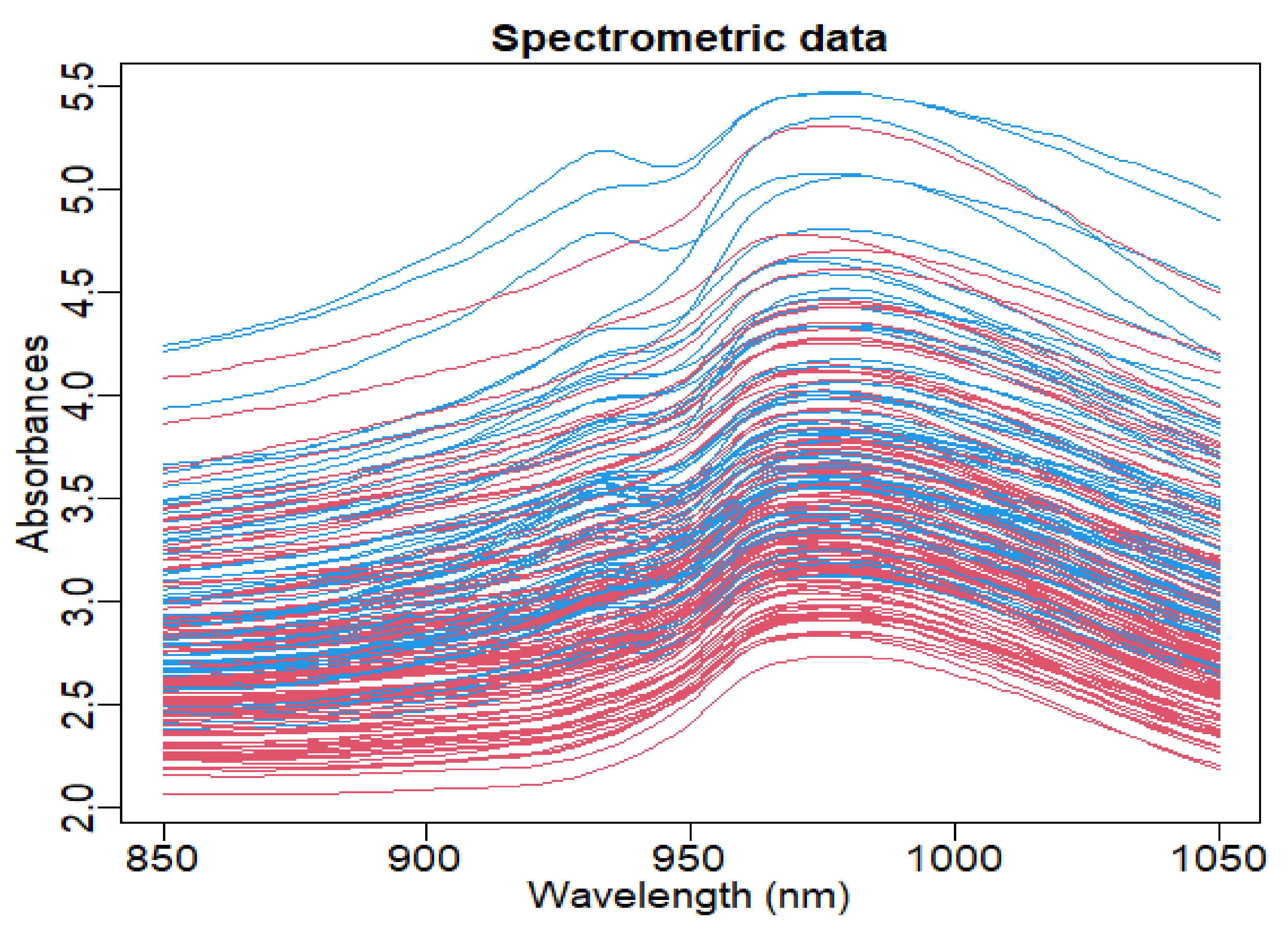
Given 215 finely chopped pieces of meat, Tecator’s data contain their corresponding fat contents ($Y_i,i=1,\dots ,215$), near-infrared absorbance spectra ($Z_i,i=1,\dots ,215$) observed on 100 equally wavelengths in the range 850–1050 nm, the protein content $X_{1,i}$ and the moisture content $X_{2,i}$. We are trying to predict the fat content of the finely chopped meat samples.

The following figure (Figure 5) shows the absorbance curves.

We divide the sample randomly into two sub-samples: the training $I_1$ of size 160 and the test $I_2$ of size 55. The training sample is used to estimate the parameters, and the test sample is employed to verify the quality of predictions. To perform our model, we use the mean square error of prediction (MSEP) like in Aneiros-Pérez and Vieu [11] defined as follows:

$${\displaystyle MSEP=\frac{1}{50}\sum _{i\in I_2}{(Y_i-{\widehat{Y}}_i)}^2/va{r}_{I_2}\left(Y_i\right),}$$

where ${\widehat{Y}}_i$ is the predicted value based on the training sample and $va{r}_{I_2}$ is variance of response variables’ test sample.

The following table (

Table 17. The MSEPs for different models.

Functional Models	MSEP
Model 1 (PLGSIMF) ${\displaystyle g\left(\mu (X_i,Z_i)\right)=\eta ({\alpha }_1{X}_{1,i}+{\alpha }_2{X}_{2,i})+{\int }_{850}^{1050}\beta \left(t\right)Z_i\left(t\right)dt}$	0.015
Model 2 (GFPLM) ${\displaystyle g\left(\mu (X_i,Z_i)\right)={\alpha }_1{X}_{1,i}+{\alpha }_2{X}_{2,i}+{\int }_{850}^{1050}\beta \left(t\right)Z_i\left(t\right)dt}$	0.024
Model 3 (GFPLM) ${\displaystyle g\left(\mu (X_i,Z_i)\right)=\eta \left(X_{1,i}\right)+{\int }_{850}^{1050}\beta \left(t\right)Z_i\left(t\right)dt}$	0.029
Model 4 (GFPLM) ${\displaystyle g\left(\mu (X_i,Z_i)\right)=\eta \left(X_{2,i}\right)+{\int }_{850}^{1050}\beta \left(t\right)Z_i\left(t\right)dt}$	0.046
Model 5 (GFLM) ${\displaystyle g\left(\mu (X_i,Z_i)\right)={\int }_{850}^{1050}\beta \left(t\right)Z_i\left(t\right)dt}$	0.051
Model 6 (SIM) $Y_i=\eta ({\alpha }_1{X}_{1,i}+{\alpha }_2{X}_{2,i})+{\epsilon }_i$	1.112

) shows the performance of our PLGSIMF model by comparing it with other models. We can conclude that PLGSIMF is competitive one for such data.

The following figure (Figure 6) shows us the estimator of the non-parametric function $\widehat{\eta }(.)$.

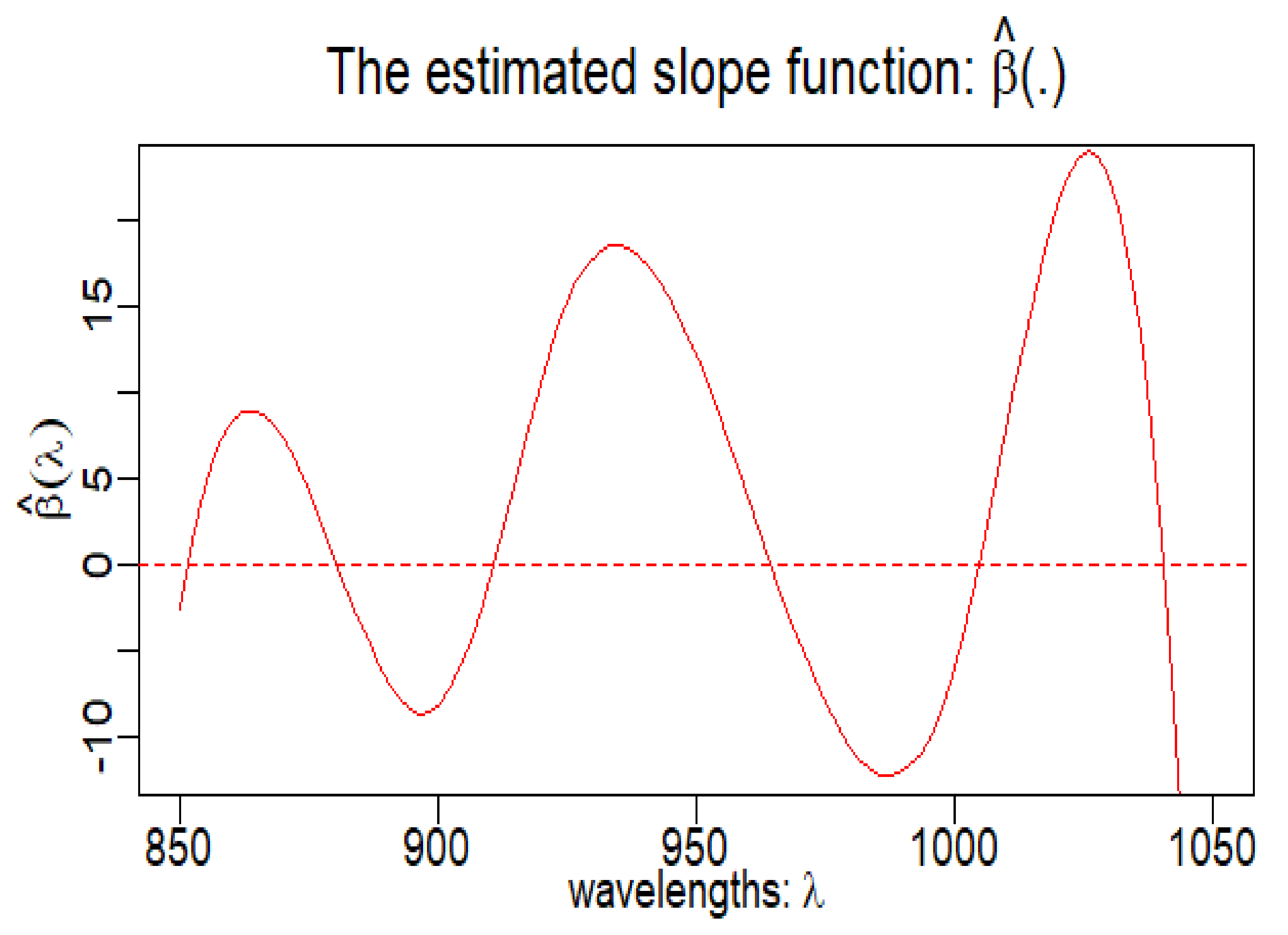
The following figure (Figure 7) shows us the estimator of the slope function $\widehat{\beta }(.)$.

6. Proofs

In what follows, when no confusion is possible, we will denote by C a generic positive constant.

The following lemmas, [21,22,23] will be used to prove Theorem 1. The proof of these lemmas will be developed in the Appendix A.

Lemma 1.

Under assumptions(C1)–(C4)and(C6)–(C8), we have

$$\sqrt{n}\left(\begin{array}{c}\tilde{\tau }-{\tau }_0\\ \tilde{\delta }-{\delta }_0\end{array}\right)\stackrel{D}{⟶}\mathcal{N}\left(0,A^{-1}{\Sigma }_1{A}^{-1}\right),$$

where ${\Sigma }_1$ and A will be defined below and in the appendix for more details.

$\stackrel{D}{\to }$ denotes the convergence in distribution.

$A=\left(\begin{array}{cc}{A}_{11}& A_{12}\\ A_{12}^{\top }& A_{22}\end{array}\right).$with

$$\begin{array}{ccc}\hfill A_{11}& =& \mathbb{E}\left[{\rho }_2\left(m_o\left(T\right)\right){\left\{{\eta }_0^{\prime }\left(U_{\tau ,0}\right)\right\}}^2{J}^{\top }\left({\tau }_0\right)X{W}^{\top }J\left({\tau }_0\right)\right]\hfill \\ \hfill A_{22}& =& \mathbb{E}\left[{\rho }_2\left(m_0\left(T\right)\right)W{W}^{\top }\right]\hfill \\ \hfill A_{12}& =& \mathbb{E}\left[{\rho }_2\left(m_o\left(T\right)\right){\eta }_0^{\prime }\left(U_{\tau ,0}\right)J^{\top }\left({\tau }_0\right)X{W}^{\top }\right]\hfill \end{array}$$

$${\Sigma }_1=\mathbb{E}\left[q_1^2\left(m_0\left(T\right),Y\right)\left(\begin{array}{c}{\eta }_0^{\prime }\left(U_{\tau ,0}\right)J^{\top }\left({\tau }_0\right)X\\ Z\end{array}\right){\left(\begin{array}{c}{\eta }_0^{\prime }\left(U_{\tau ,0}\right)J^{\top }\left({\tau }_0\right)X\\ Z\end{array}\right)}^{\top }\right]$$

By applying the $\delta$-method, we get the following lemma.

Lemma 2.

Under the conditions of Lemma 1, we obtain

$$\sqrt{n}\left(\begin{array}{c}\alpha \left(\tilde{\tau }\right)-\alpha \left({\tau }_0\right)\\ \tilde{\delta }-{\delta }_0\end{array}\right)\stackrel{D}{⟶}\mathcal{N}\left(0,R\left({\tau }_0\right)A^{-1}{\Sigma }_1{A}^{-1}{R}^{\top }\left({\tau }_0\right)\right),$$

where

$$R\left(\tau \right)=\left(\begin{array}{cc}J\left(\tau \right)& 0\\ 0& I_{N^{\prime }\times N^{\prime }}\end{array}\right).$$

Furthermore ${\displaystyle \alpha \left(\tilde{\tau }\right)-\alpha \left({\tau }_0\right)=o_{\mathrm{I}\mathrm{P}}\left(\frac{1}{\sqrt{n}}\right)}$ and ${\displaystyle \tilde{\delta }-{\delta }_0=o_{\mathrm{I}\mathrm{P}}\left(\frac{1}{\sqrt{n}}\right)}$.

Lemma 3.

Under the conditions of Lemma 1, we obtain

$$\parallel \widehat{\theta }-\tilde{\theta }\parallel ={\mathcal{O}}_{\mathrm{I}\mathrm{P}}\left(\sqrt{N_n}\left(h^p+\frac{1}{\sqrt{nh}}\right)\right),$$

where $N_n$ is number of B-splines basis functions of order r.

Then, we can enounce the following theorem.

Theorem 4.

Under assumptions(C1)–(C5)and(C6)–(C8), we obtain

$${∥\widehat{\eta }-{\eta }_0∥}_2={\mathcal{O}}_{\mathrm{I}\mathrm{P}}\left(\sqrt{N_n}\left(\frac{1}{\sqrt{n}h}+h^p\right)\right),$$

and

$${∥\widehat{\eta }-{\eta }_0∥}_n={\mathcal{O}}_{\mathrm{I}\mathrm{P}}\left(\sqrt{N_n}\left(\frac{1}{\sqrt{n}h}+h^p\right)\right).$$

Theorem 5.

Under assumptions(C1)–(C8), and $k\sim n^{1/(2r+1)}$, we obtain

$$\parallel \widehat{\beta }(·)-{\beta }_0{(·)\parallel }^2={\mathcal{O}}_{\mathrm{I}\mathrm{P}}\left(N_n^2{\left(h^p+\frac{1}{\sqrt{nh}}\right)}^2\right)+{\mathcal{O}}_{\mathrm{I}\mathrm{P}}\left(n^{-2r/(2r+1)}\right).$$

Theorem 6.

Under assumptions $\left(C_1\right)-\left(C_{11}\right)$, the constrained quasi-likelihood estimators $\widehat{\alpha }$ and $\widehat{\delta }$ with $\parallel \widehat{\alpha }{\parallel }_d=1$ is asymptotically normally distributed, i.e.,

$$\sqrt{n}\left(\begin{array}{c}\widehat{\alpha }-{\alpha }_0\\ \widehat{\delta }-{\delta }_0\end{array}\right)\stackrel{D}{⟶}\mathcal{N}\left(0,R\left({\tau }_0\right)D^{-1}{R}^{\top }\left({\tau }_0\right)\right)$$

where

$$D=\mathbb{E}\left[{\rho }_2\left(m_0\left(T\right)\right)\left(\begin{array}{c}{\eta }_0^{\prime }\left(U_{\tau ,0}\right)J^{\top }\left({\tau }_0\right)\Phi \left(X\right)\\ \Psi \left(W\right)\end{array}\right){\left(\begin{array}{c}{\eta }_0^{\prime }\left(U_{\tau ,0}\right)J^{\top }\left({\tau }_0\right)\Phi \left(X\right)\\ \Psi \left(W\right)\end{array}\right)}^{\top }\right].$$

Notice that the proof of this theorem is very long. So, in order to save space and not to make this paper more difficult to read, we opted for adding a Supplementary Materials, containing necessary details.