Article

Some New Tests of Conformity with Benford’s Law

1
Department of Social and Economic Sciences, Sapienza University of Rome, P.le Aldo Moro 5, I-00185 Rome, Italy
2
Department of Economics, University of Molise, Via De Sanctis snc, I-86100 Campobasso, Italy
*
Author to whom correspondence should be addressed.
London South Bank University Business School, 103 Borough Road, London SE1 0AA, UK.
Stats 2021, 4(3), 745-761; https://doi.org/10.3390/stats4030044
Submission received: 19 July 2021 / Revised: 1 September 2021 / Accepted: 2 September 2021 / Published: 6 September 2021
(This article belongs to the Special Issue Benford's Law(s) and Applications)

Abstract

:
This paper presents new perspectives and methodological instruments for verifying the validity of Benford’s law for a large given dataset. To this aim, we first propose new general tests for checking the statistical conformity of a given dataset with a generic target distribution; we also provide the explicit representation of the asymptotic distributions of the relevant test statistics. Then, we discuss the applicability of such novel devices to the case of Benford’s law. We implement extensive Monte Carlo simulations to investigate the size and the power of the introduced tests. Finally, we discuss the challenging theme of interpreting, in a statistically reliable way, the conformity between two distributions in the presence of a large number of observations.

1. Introduction

Data regularities are relevant properties of many datasets whose elements maintain their individuality while creating a unified framework. One of the most illustrative examples of such statistical features is that of Benford’s law, introduced in [1] and successfully tested and described in [2]. Benford’s law is a sort of magic rule, for which the first digit(s) of the elements of a given dataset follow a specific distribution—hereafter called Benford’s distribution. For all the details on such a law, we refer the interested reader to [3,4,5,6].
Benford’s law is not at all intuitive; however, over the years, long after Frank Benford’s paper appeared (see [2]), several solid theoretical motivations and explanations have been found, mathematically validating the phenomenon (see, among others, refs. [4,5,7,8,9,10,11,12]). Surprisingly, this digital pattern holds true in a large number of cases, with datasets in the fields of economics (e.g., [13,14,15,16]), accounting (e.g., [17,18,19]), finance (e.g., [20,21,22,23,24,25]), geophysics and hydrology (e.g., [26,27,28]), as well as social sciences (e.g., [29,30,31]).
A methodological aspect of Benford’s law lies in how to test the compliance of the empirical distribution of a given sample with Benford’s variable. The root of such an issue lies in the definition of a statistical distance between two random variables, the most popular being the chi-square and the mean absolute deviation (MAD).
This paper deals with this challenging research theme. Specifically, we advance herein some new tests for verifying the compliance of the empirical distribution obtained from a given population. In this respect, we mention the recent contribution [32], where the authors suggested a statistical test based on the mean. Following the quoted paper, we start by introducing a mean-based conformity test. Moreover, we also developed a variance-based and a joint mean and variance-based test for verifying the compliance of a given distribution with a target one. Furthermore, we also present a test based on Wald’s statistic and a new version of a MAD-based test. We explored the asymptotic distributions of the proposed tests; furthermore, we pay specific attention to their size and power, which were investigated through a large set of Monte Carlo simulations.
We also focus the so-called “excess of power problem”. In this respect, we mention Kossovsky’s criticism ([12], in this Special Issue), where the author refers to the “mistaken use of the Chi-Square test in Benford’s law”. From this perspective, we also mention the theme of the selection of the critical thresholds for having perfect/marginal/acceptable conformity with Benford’s law (see [3,4] and the recent study developed by [33]). Finally, the problem of the “excess of power problem” is treated using resampling techniques.
The rest of the paper is organised as follows: the next Section introduces the new tests and derives their asymptotic null distribution; Section 3 illustrates the extensive Monte Carlo analysis carried out to investigate the size and power properties of the proposed tests in the relevant cases of the first digit and first two digits Benford’s law; the “excess of power problem” is addressed in Section 4; the last Section draws some conclusions. An Appendix reports some further technical details.

2. New Tests of Conformity with Benford’s Law

In this Section, we report the analytical derivations of the new test statistics of conformity to Benford’s law and their asymptotic distributions.
Proposition 1. 
Consider a random sample x 1 , , x n from a population with mean μ, variance σ 2 , and third and fourth central moments μ 3 and μ 4 . All moments up to the fourth are assumed to be finite. Let x ¯ n and s n 2 be the sample mean and the sample variance, respectively. Then:
x ˜ n : = n x ¯ n μ σ   d N ( 0 , 1 ) ;
s ˜ n 2 : = n s n 2 σ 2 μ 4 σ 4   d N ( 0 , 1 ) ;
n μ σ : = x ˜ n + s ˜ n 2 2 1 + μ 3 σ μ 4 σ 4 1 2   d N ( 0 , 1 ) ;
w μ σ : = x ˜ n , s ˜ n 2 1 μ 3 σ μ 4 σ 4 μ 3 σ μ 4 σ 4 1 1 x ˜ n s ˜ n 2 = z n 1 z n   d χ 2 ( 2 ) ,
with z n denoting the transpose of z n .
Proof. 
To prove (1) and (2) see, e.g., [34] (Theorem 10.1).
To prove (3), first note that:
cov ( x ˜ n , s ˜ n 2 ) = n σ n μ 4 σ 4 cov ( x ¯ n , s n 2 )
= n σ μ 4 σ 4 μ 3 n
= μ 3 σ μ 4 σ 4
where cov ( x ¯ n , s n 2 ) = μ 3 / n see [35]; (3) then follows from (1) and (2) and from the rule of the variance of a sum of correlated random variables.
Let us now define z n : = ( x ˜ n , s ˜ n 2 ) . The Cramér–Wold device implies that z n is (asymptotically) multivariate normal if λ z n is (asymptotically) univariate normal for every λ R 2 . However, every λ R 2 defines a linear combination of two (asymptotically) normal variables and λ z is trivially (asymptotically) univariate normal. Therefore:
n x ˜ n s ˜ n 2   d N 0 0 , 1 μ 3 σ μ 4 σ 4 μ 3 σ μ 4 σ 4 1 N ( 0 , )
and (4) follows. □
Remark 1. 
The results stated in Proposition 1 can be used to test conformity (goodness of fit) with any given distribution with finite moments up to the fourth. If μ, σ, μ 3 , and μ 4 are those of Benford’s distribution, then Equation (1) can be used to build a conformity test based on the mean: such a test has indeed recently been suggested by Hassler and Hosseinkouchack [32]. Equation (2) is the basis for a normal conformity test based on the variance, whereas (3) can be used to build a normal conformity test jointly based on the mean and the variance. Finally, (4) is a chi-square conformity test which jointly considers the mean and the variance.
Remark 2. 
When conformity is tested with reference to the normal distribution, (4) is simplified because μ 3 = 0 : indeed, under normality, the sample mean and the sample variance are independent: the sample mean and the sample variance are not independent random variables for any other distribution, as can be seen in [36].
Proposition 2. 
Consider a random sample x 1 , , x n from a discrete random variable with k n classes with individual probabilities p : = ( p 1 , , p k ) , with p j 0 j { 1 , , k } . Let f n : = ( f n 1 , f n k ) be a consistent estimate of p and define e n : = ( e n 1 , , e n k ) = f n p and : = diag ( p ) p p . Then:
w : = n e n * * 1 e n *   d χ 2 ( k 1 )
where e n * : = ( e n 1 , , e n , k 1 ) and * is made of the first k 1 rows and columns of . Furthermore:
M A D : = n k j = 1 k f n j p j p j ( 1 p j )   d N 2 π , 1 k 2 i = 1 k j = 1 k r i j
where:
r i j = 2 π ρ i j arcsin ( ρ i j ) + 1 ρ i j 2 2 π
and:
ρ i j = p i p j ( 1 p i ) ( 1 p j ) .
Proof. 
To prove (9), let Y i j : = 1 X i = j with 1 κ being the indicator function which is equal to 1 when condition κ is satisfied and 0 otherwise. Furthermore, Y i j Bern ( p j ) and S n j : = i = 1 n Y i j Binom n p j , n p j ( 1 p j ) . Then:
e n j : = S n j n p j n p j ( 1 p j ) = n S n j n p j p j ( 1 p j ) = n f n j p j p j ( 1 p j ) = n e n j p j ( 1 p j )   d N ( 0 , 1 )
by the central limit theorem. Furthermore, the covariance matrix of e n is = diag ( p ) p p , as can be seen in [37]. Again invoking the Cramér–Wold device n   e   d N ( 0 , ) and (9) is a Wald-like statistic with a χ 2 ( k 1 ) limiting distribution under the null [38] (p. 71).
To prove (10), we exploit the fact that if Y ( 0 , 1 ) , then see [36]:
E | Y | = 2 π .
Furthermore:
var ( | Y | ) = E ( | Y | 2 ) E ( | Y | ) 2 = 2 π 0 y 2 e y 2 2 d y 2 π = 1 2 π .
Therefore, by (13):
n e n j : = n f n j p j p j ( 1 p j )   d N 2 π , 1 2 π .
Furthermore, n e n : = n ( e n 1 , , e n k )   d N ı 2 π , R by the Cramér–Wold device, with ı a k-vector of ones.
Using the fact that when ( X , Y ) have a bivariate normal distribution with means 0, variances ı and correlation θ , then [39]:
E | X | | Y | = 2 π θ arcsin ( θ ) + 1 θ 2
and therefore:
E | e n i | | e n j | = 2 π ρ i j arcsin ( ρ i j ) + 1 ρ i j 2
where ρ i j is the correlation between e n i and e n j :
ρ i j = p i p j ( 1 p i ) ( 1 p j ) .
Then, note that:
cov | e n i | | e n j | = E | e n i | | e n j | E | e n i | E | e n j | = 2 π ρ i j arcsin ( ρ i j ) + 1 ρ i j 2 2 π .
Therefore, the covariance matrix R is:
R = r 11 r 12 r 1 k r 12 r 22 r 2 k r 1 k r 2 k r k k = r i j
with:
r i j = 2 π ρ i j arcsin ( ρ i j ) + 1 ρ i j 2 2 π .
Finally:
n k j = 1 k e n j = 1 k j = 1 k n f n j p j p j ( 1 p j )   d N 2 π , 1 k 2 ı R ı .
Remark 3. 
The results stated in Proposition 2 can be used to test conformity (goodness of fit) with any given discrete distribution and specialise to the first digit or first two digits Benford’s law when p i = log 10 ( 1 + 1 / d ) , with either d = 1 , , 9 or d = 10 , , 99 . Here, (9) is a Wald-like test, whereas (10) is a modification of the mean absolute deviation (MAD) statistic advocated in [3,40], where each absolute deviation is adjusted by the factor 1 / p j ( 1 p j ) thereby emphasising deviations from smaller expected frequencies, as well as incorporating (the square root of) the sample size n as a factor in the measure of deviation.
Remark 4. 
The Wald-like χ 2 statistic in (9) is equivalent to the usual χ 2 computed as n j = 1 k e n j 2 / p j . A proof, which also proves that * is nonsingular, is offered in Appendix A.
Remark 5. 
Equation (10) makes it clear that, contrarily to what is commonly asserted, as can be seen in, e.g., [3] (p. 158), the M A D statistic:
M A D : = 1 k j = 1 k f n j p j
is not independent of n and is, in fact, O p n 1 2 .

3. Monte Carlo Simulations

The size (the probability of falsely rejecting the null hypothesis) and power (the ability of the test to reject the null when it is false) of the proposed tests are investigated over 25,000 Monte Carlo replications for varying sample sizes n, under the null and under selected interesting alternatives (all computations and graphics were produced using R, version 4.0.5 [41] and ggplot2, version 3.3.3 [42]). Each alternative is expressed in terms of the mixture:
p = λ p B + ( 1 λ ) p A
where p B : = ( p B 1 , , p B k ) is the vector of Benford’s probabilities, p A : = ( p A 1 , , p A k ) is the vector of probabilities of some “contaminating” distribution, and k is the number of digits. λ { 0.75 , 0.80 , , 0.95 } is the mixing parameter. When dealing with data manipulation issues, 1 λ can be interpreted as the fraction of manipulated data.
The following mixtures were used in the simulations:
  • Uniform mixture: p A describes the discrete uniform distribution with the same support as the considered Benford’s distribution;
  • Normal mixture: p A i are the probabilities of N ( μ B , σ 2 ) , with μ B the mean of Benford’s distribution and σ = 4 μ B ;
  • Randomly perturbed mixture: Benford’s law is perturbed by a random quantity in correspondence to each digit. More precisely, p A i = u i p B i with u i U ( 0 , 2 p B i ) . Since this mixture contains elements of randomness, each Monte Carlo iteration uses a different mixture. However, the mixtures are the same across all tests;
  • Under-reporting mixture: under the alternative, Benford’s distribution is modified by putting to zero the probability of “round” numbers and giving this probability to the preceding number: for example, p A 20 = 0 and p A 19 = p B 19 + p B 20 . This mixture is only considered with reference to the first two digits case.
The above mixtures are plotted in Figure 1 for the first two-digit case. The corresponding data for each mixture are generated from a multinomial distribution with vector probability. In order to reduce Monte Carlo variability, all tests were applied to the same data, and larger samples include observations from the smaller ones.
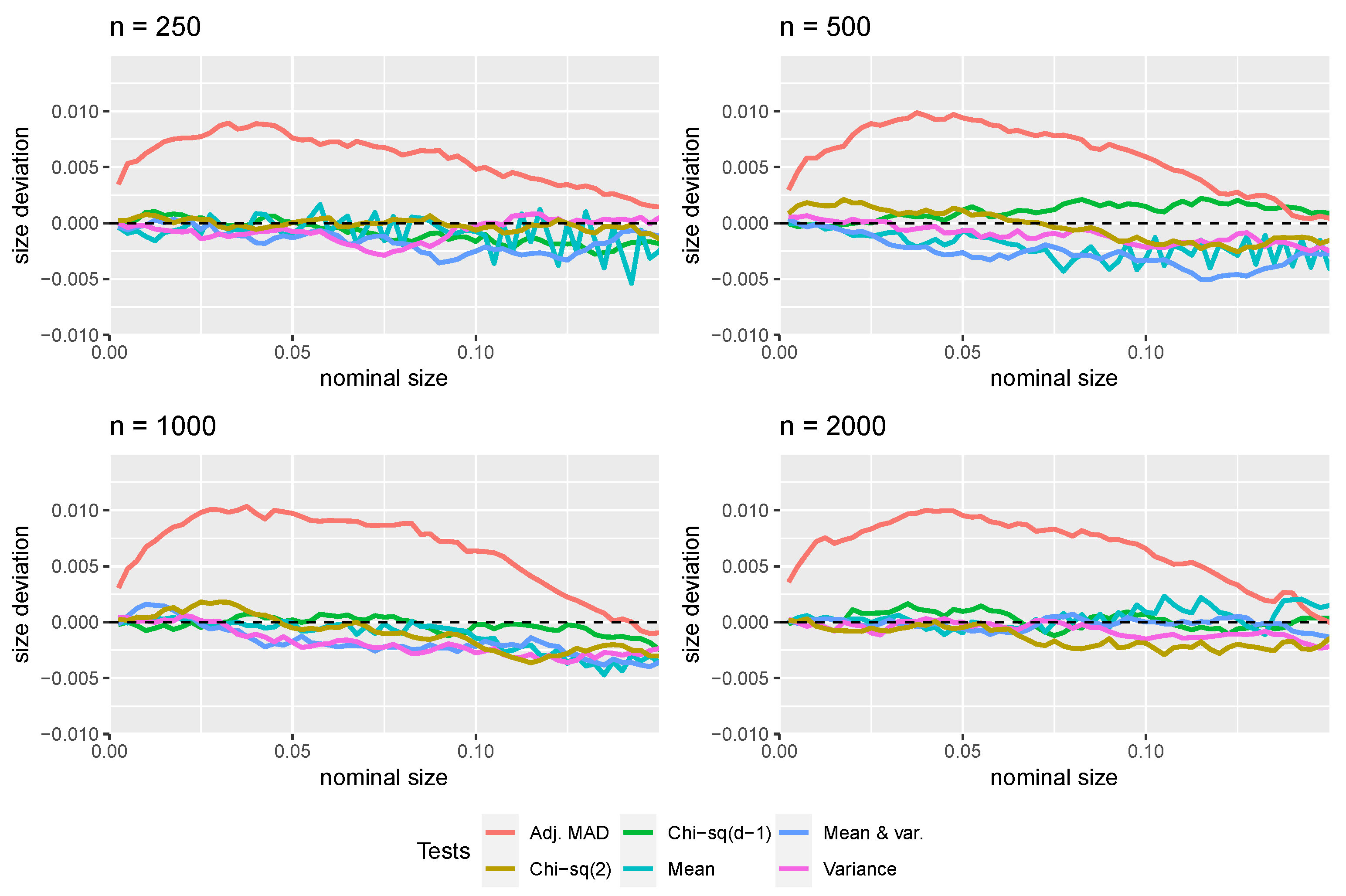
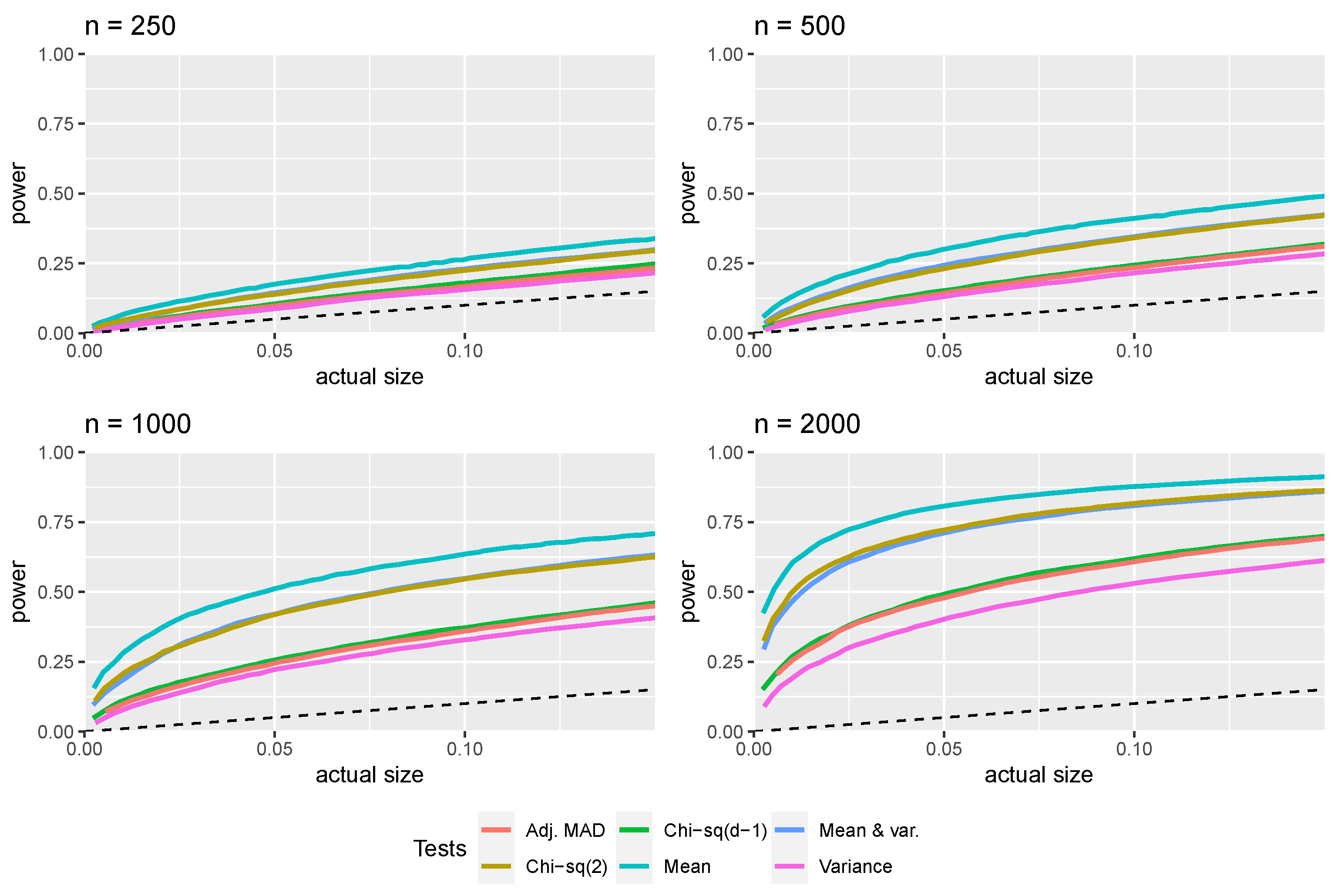
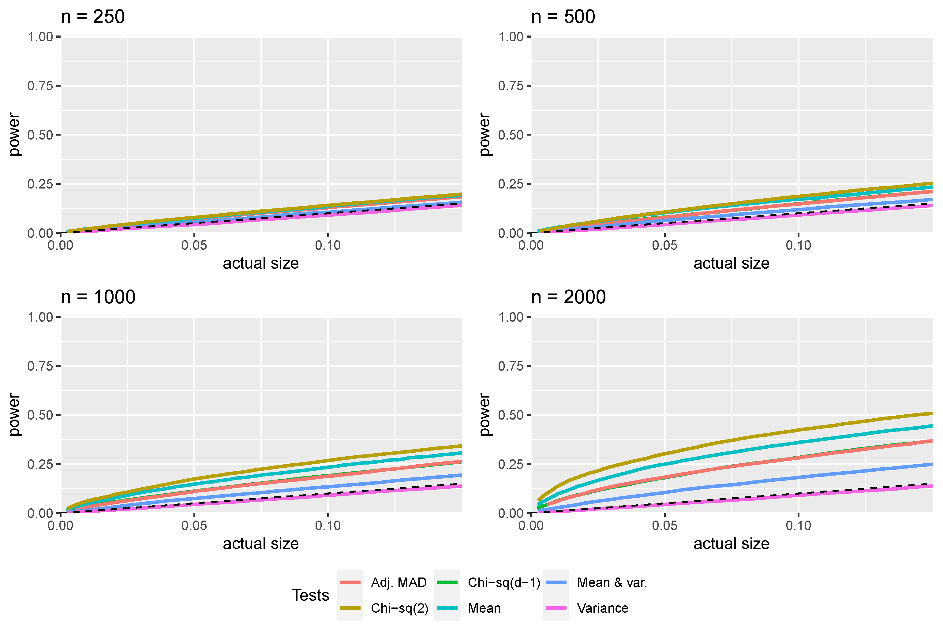
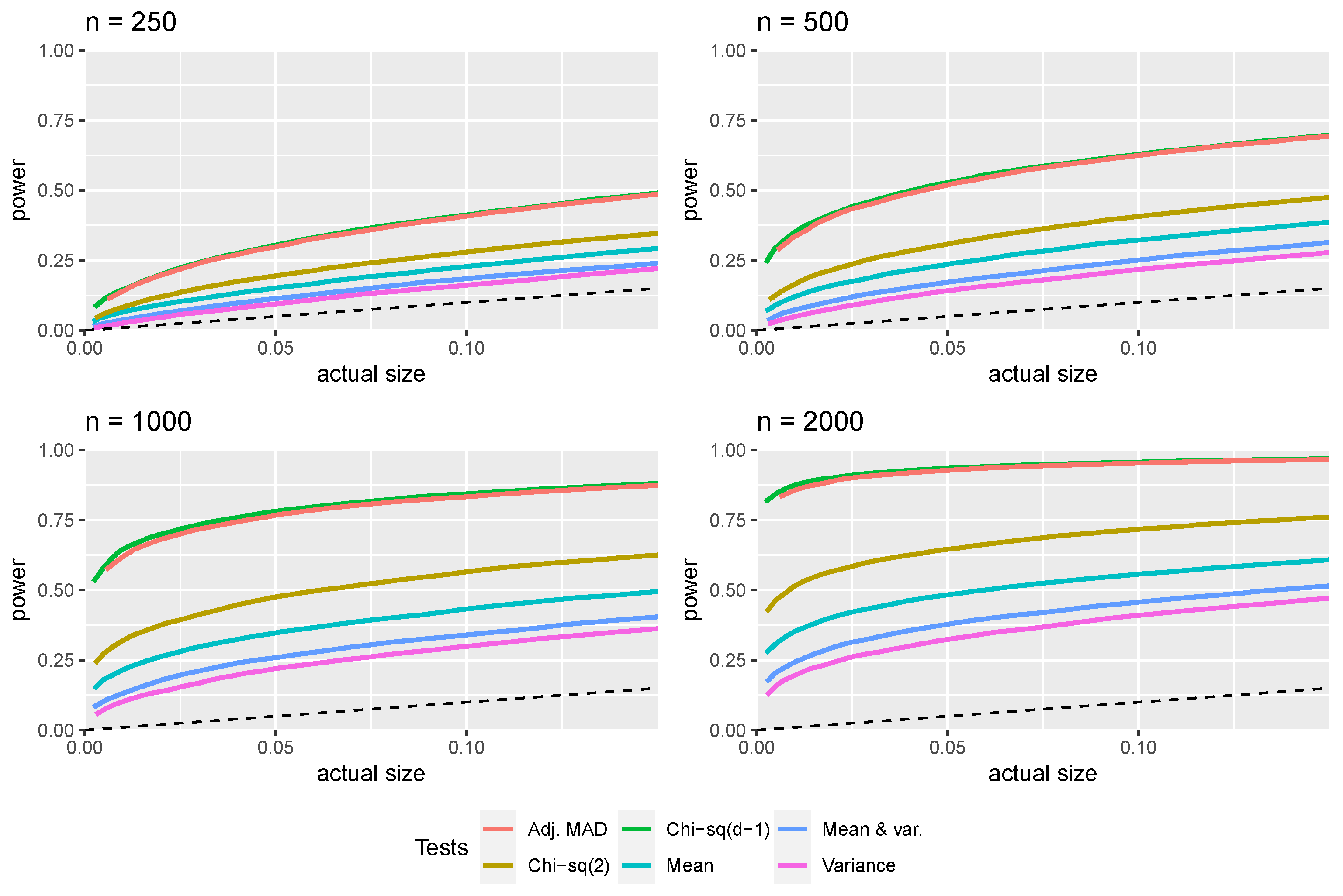
Rather than reporting long and difficult-to-compare tables of outcomes, we summarise the simulation results by relying on a graphical approach (as can be seen in, e.g., [43,44]). In order to summarise the size properties of the tests, we plot the size deviations (i.e., a c t u a l s i z e n o m i n a l s i z e ) against nominal size. When no size distortions are present, a c t u a l s i z e = n o m i n a l s i z e , and this graph coincides with a horizontal line with the ordinate equal to zero; however, this is a theoretical case only, since in practice, size deviations will tend to reflect experimental randomness. To report power results, we use size–power curves: these curves allow us to easily visualise the power of each test in correspondence of its actual (rather than nominal) size and to compare the power of different tests on perfectly fair grounds. The line p o w e r = a c t u a l s i z e is also reported as a reference, representing the performance of a test of no practical use (the fraction of rejections under the null and under the alternative is the same); the more distant the size–power curve is from this line, the more powerful the test is.

3.1. First-Digit Law

The tests generally have very good size properties, irrespective of the sample size, with size deviations of approximately zero (see Figure 2). Only the modified MAD test tends to over-reject slightly under the null (with a +0.01 deviation with respect to nominal size) in correspondence of the 5% nominal size. In other words, the actual size of the modified MAD test in correspondence of the 5% nominal size is around 6%, and the discrepancy tends to reduce for larger nominal sizes.
As far as power is concerned, the performance of the different tests depends on the specific alternative hypothesis considered. The normal mean test (1) is the most powerful in the presence of a uniform mixing alternative (Figure 3), followed by the χ 2 ( 2 ) test on the mean and the variance (4) and the normal test on the mean and the variance (3).
In the presence of a normal mixing alternative (Figure 4), the χ 2 ( 2 ) (4) and the normal test on the mean (1) perform the best, followed by the adjusted MAD (10) and the Wald-like χ 2 ( d 1 ) test (9).
Finally, in the presence of a perturbed Benford distribution (Figure 5), the highest power is reached by the χ 2 ( d 1 ) (9) and the adjusted MAD (10) tests, followed by the χ 2 ( 2 ) test (4).

3.2. First Two Digits Law

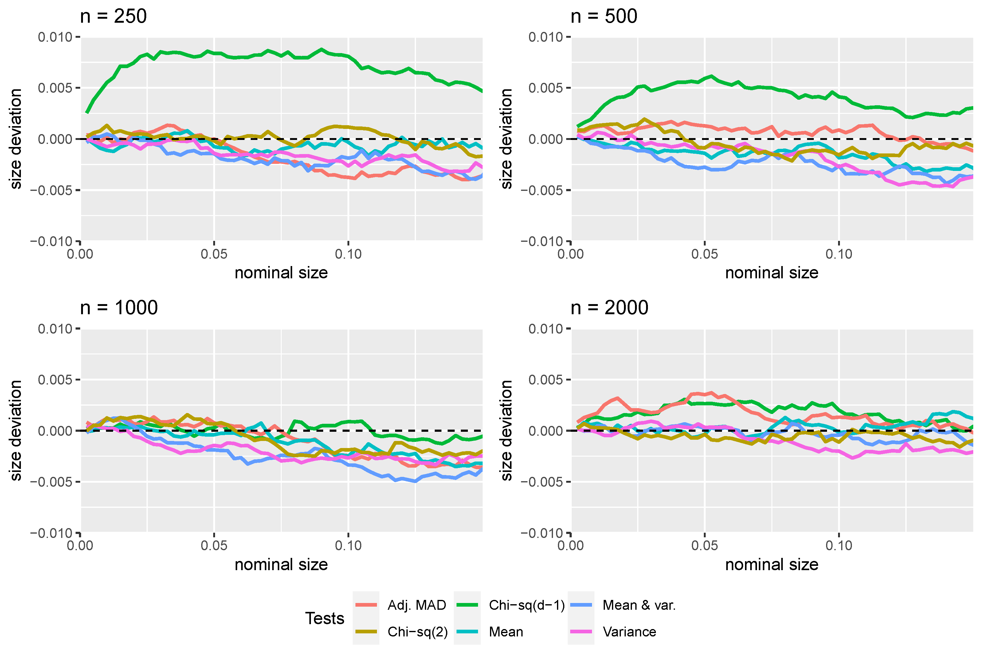
All the tests have approximately the correct size, even in the presence of fairly small samples (see Figure 6). All deviations with respect to the nominal size are within ± 0.005 , with the only exception of the ordinary chi-square test which shows a deviation around 0.010 in correspondence with values of the nominal size of common usage for n = 250 .
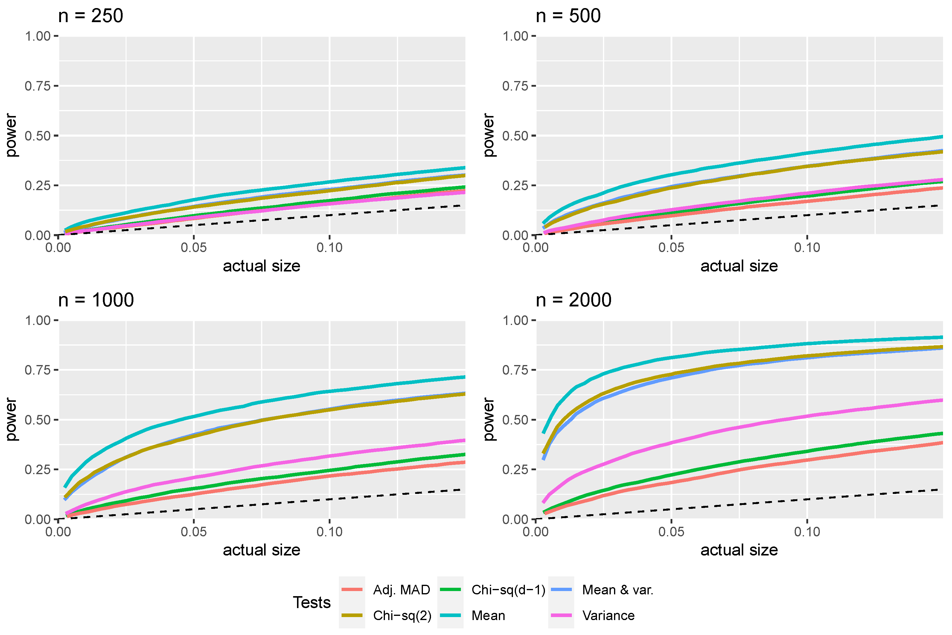
As anticipated, the power performance of the tests crucially depends on the alternative. The normal test based on the mean (1) is the most powerful test among those considered here, in the presence of a uniform mixing alternative (see Figure 7). The χ 2 ( 2 ) test on the mean and variance (4) and the normal test on the mean and variance (3) followed at short distance.
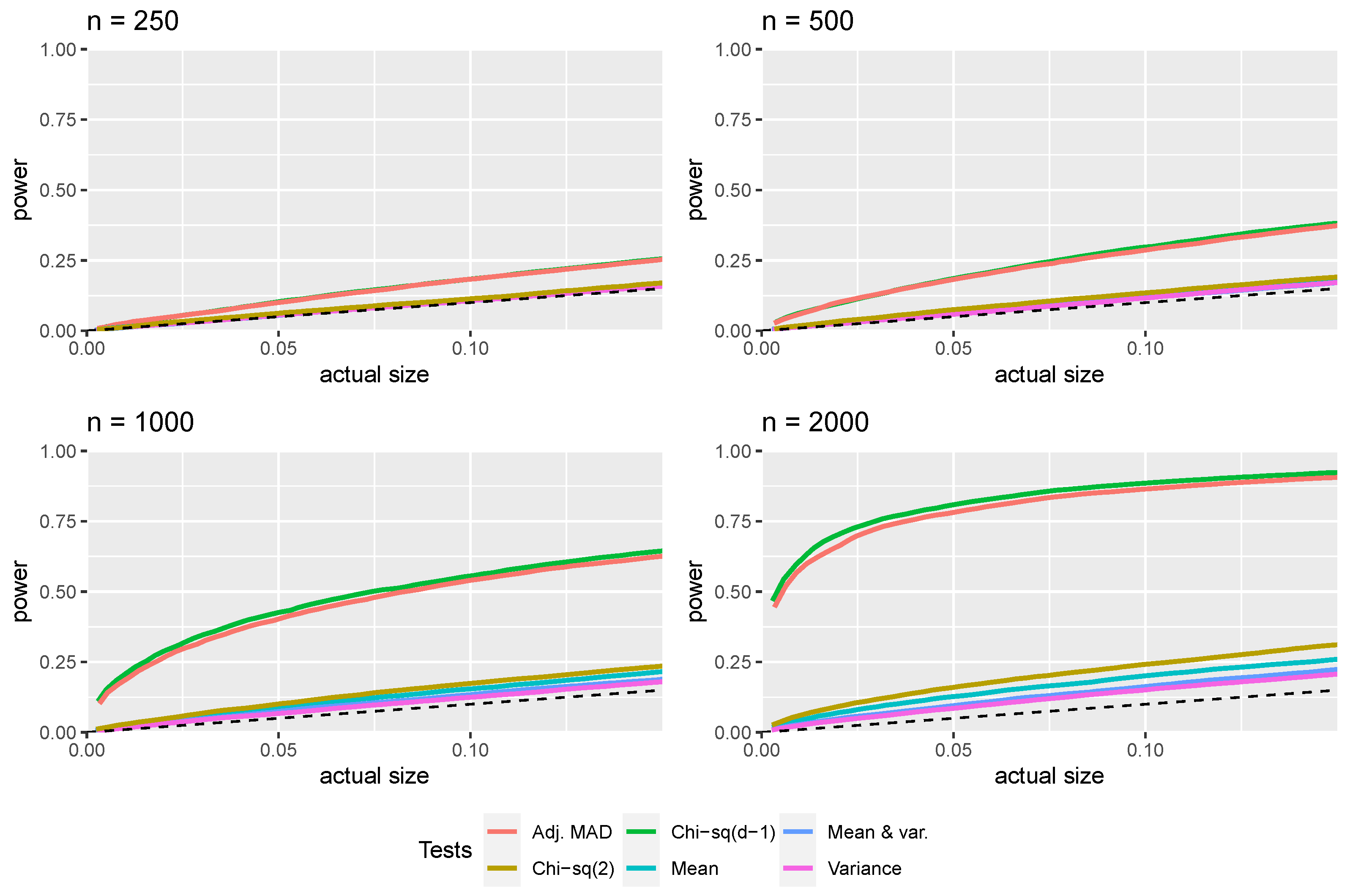
In the presence of a normal mixing alternative (see Figure 8), the χ 2 ( 2 ) test (4) is the most powerful one, followed by the normal variance test (2). It is interesting to note that in the first digit case, the normal variance test had no power; here, the normal mean test has no power. The other tests are generally more powerful in the first two digits than in the first digit case.
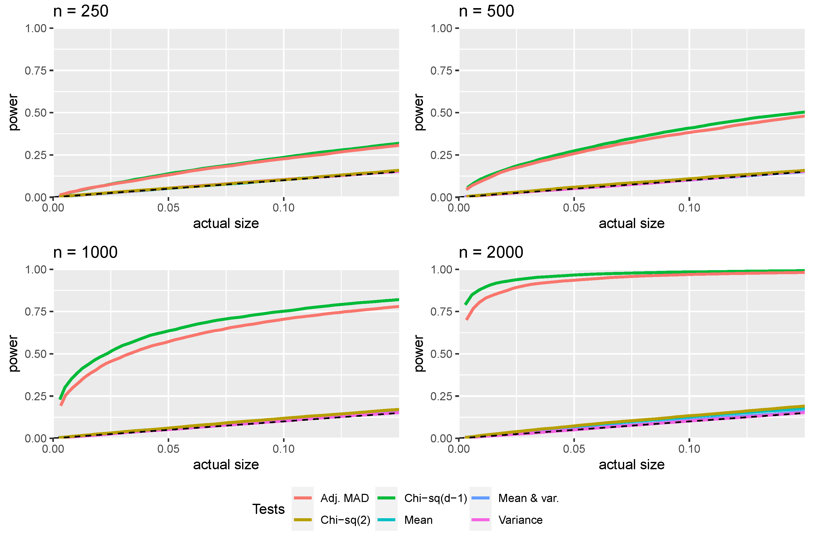
When the alternative can be described as a “perturbed Benford” distribution (Figure 9) or in terms of a rounding behaviour (Figure 10), then the χ 2 ( d 1 ) , either in the “classical” or in the equivalent Wald’s formulation (9), and the modified MAD (10) perform very closely and are by far the most powerful tests. The ordering of the tests is the same as in the first digit case; however, the tests are generally more powerful in the first digit case.
These results suggest that in applications it is generally a good idea not to rely on a single test, but to use a battery of different tests designed to detect particular deviations from the null.

4. Statistical versus Practical Significance

In 1998, Granger [45] (p. 260) pointed out that in the presence of very large datasets:
“Virtually all specific null hypotheses will be rejected using present standards. It will probably be necessary to replace the concept of statistical significance with some measure of economic significance.”
This is obviously related to the fact that the power of any consistent test increases with the sample size n, i.e., π 1 as n (with π denoting the power of the test). Of course, consistency is a desirable property of any statistical test. The symmetrical case, with small n, is somewhat less relevant in empirical applications of Benford’s law where typical sample sizes are large. However, it has been observed that standard conformity tests may substantially lack power in the presence of small sample sizes (see, e.g., [12]). In our context, a large n is required to approximate the test asymptotic distributions).
In fact, the “large n problem” and some related apparently paradoxical implications were already highlighted in a paper by Lindley in 1957 [46]. The idea that a “large n problem” plagues empirical tests of conformity with Benford’s distribution is widespread in the literature on Benford’s law (as can be seen in, e.g., Nigrini’s contributions [3,40] and Kossovsky’s paper in this Special Issue [12]). In fact, Nigrini [3] (p. 158) claims that:
“What is needed is a test that ignores the number of records. The mean absolute deviation ( M A D ) test is such a test, and the formula is shown in Equation 7.7. [...] There is no reference to the number of records, N, in Equation 7.7.”
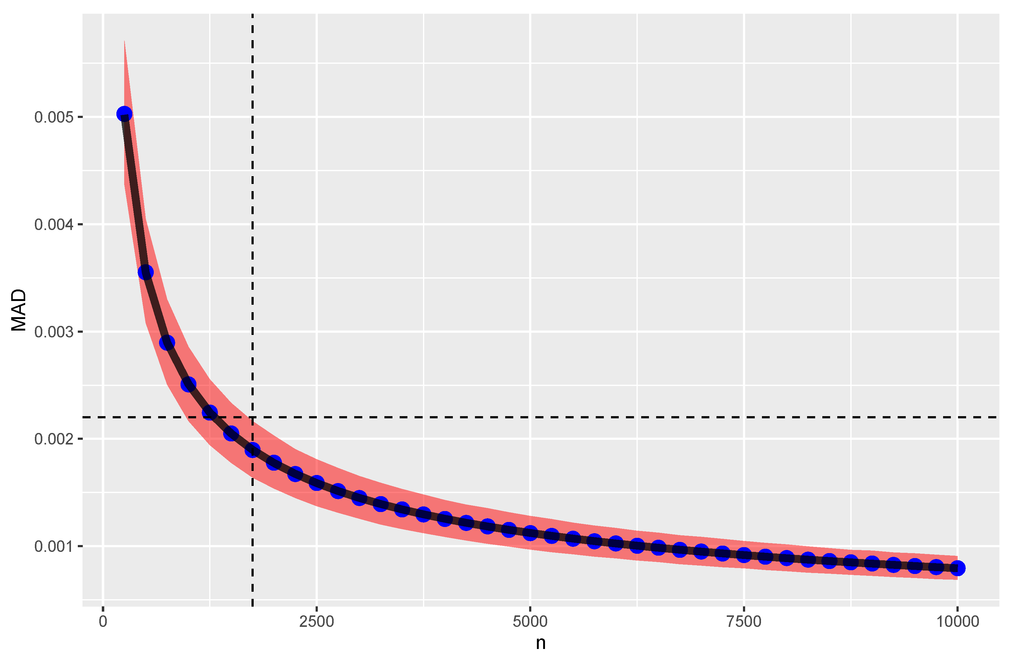
However, Nigrini’s statement that the M A D does not depend on the number of observations would only be valid if the relative frequencies of the digits for the data were given, not estimated. The fact that the relative frequencies must be estimated from the observed data makes the M A D dependent on the sample size, despite the sample size not explicitly appearing in the MAD formula. In fact, in proposition 2, we show that Nigrini’s M A D is O p n 1 2 under Benford’s distribution (see Remark 5 above). Indeed, Figure 11 clearly shows that the behaviour of the estimated M A D is perfectly consistent with 1 / n under the null: therefore, taking a fixed “critical value” for the M A D irrespective of the sample size may lead to biased conclusions.
The risk of rejecting the (Benford’s law) null hypothesis for tiny uninteresting deviations in the presence of large datasets can be dealt with in two different ways: (i) using significance levels α n decreasing with increasing n; and (ii) using a sort of “m out of n bootstrap” procedure [47] to assess significance. In what follows, we explain this second route with specific reference to the “first two digits” case.
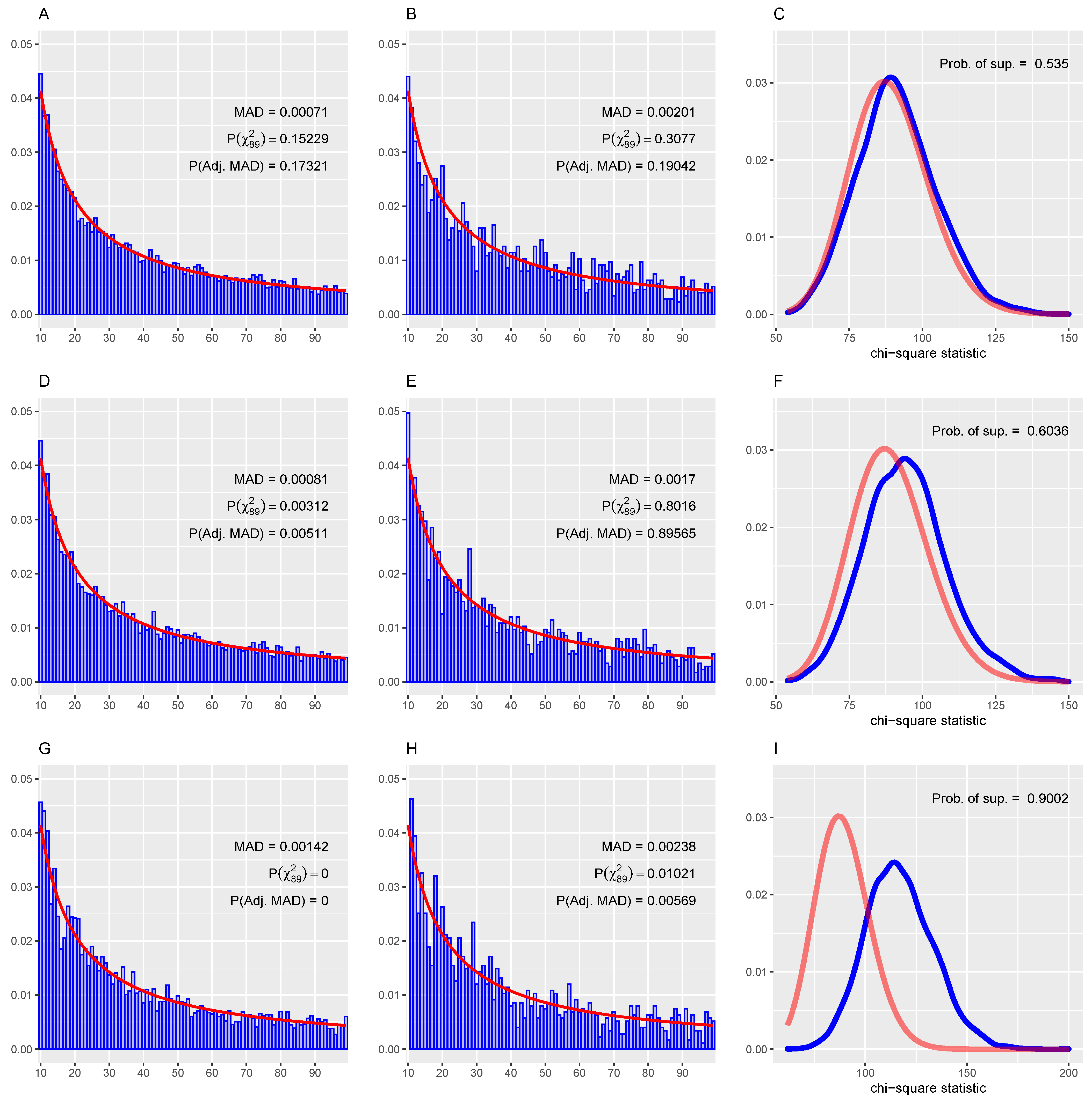
If the available sample is very large (e.g., n > 3000 ), then the idea is to repeatedly test for conformity on a large number of smaller samples randomly resampled from the original data. If the observations are independent, identically distributed (IID), then the smaller samples will have the same distribution as the original data, making it possible to check conformity on the smaller datasets. In doing so, we are sacrificing some power in order to only detect “interesting” (or sizeable) departures from the null. The fact that the test statistics are computed over a large number of random sub-samples allows us to derive the distribution of the statistics and not to rely on a single outcome. The whole procedure is exemplified in Figure 12 in the case of data conforming with the “first two digits” Benford’s law (first row in the Figure) as well as for a possibly uninteresting deviation from the null (second row) and a more substantial deviation from the null (third row). In this example, the random subsamples were made of 1750 observations, consistently with Figure 11, indicating that jointly using 0.0022 as the “critical value” for the MAD with n = 1750 ensures an approximate size of 5% to Nigrini’s test. The tests considered are the M A D and those that, according to our simulations, are the most powerful in the presence of a perturbed Benford’s alternative (see Figure 9). The third column (panels C, F, I) of Figure 12 reports the estimated densities of the conventional (or Wald) chi-square test statistic over 5000 random subsamples of length n = 1750 (blue curve) along with the χ 2 ( 89 ) null distribution (red). The probability of superiority (a measure of the effect size that corresponds to the probability that a randomly chosen point under the experimental curve is larger than a randomly chosen point under the null curve: see, e.g., [48] (Chapter 11)) is also reported to compare the two distributions.
Panels A–C in Figure 12 show that the null of conformity is not rejected: this conclusion carries over using the full sample (panel A) as well as using a single subsample (panel B) or 5000 random subsamples (panel C). The null is rejected in the full sample under the “uninteresting” alternative using either the chi-square or the adjusted M A D test, but it is not rejected using the fixed “critical value” 0.0022 for the M A D (panel D). Using the subsamples, none of the criteria are able to decidedly reject the null, suggesting that the deviation of the data from the null is tiny. When the deviation is substantial (panels G–I), the M A D still cannot reject the null in the full sample (panel G) whereas the p value of the other two tests is virtually zero. In the single subsample, all three criteria correctly reject the null of conformity (panel H) and panel I shows that the “effect size” on the chi-square test is substantial, with the probability of superiority being approximately 0.9.

5. Conclusions

This paper introduces new tests of conformance with a given distribution with first four finite moments. The tests are then specialised to the special case of the first digit and first two digits Benford’s law. An extensive Monte Carlo analysis was carried out to study the size and power properties of the tests. The results show that it can be advisable to use different tests in real applications, given that the different tests perform differently, according to the nature of the alternative hypothesis.
This paper also addresses the “excess of power” problem of the tests in the presence of very large samples: the proposed solution, based on resampling techniques, seems to be able to reconcile the evidence stemming from the MAD criterion (as can be seen in, e.g., [3]) with firmly statistically based tests.

Author Contributions

The authors equally contributed to this work. Both authors have read and agreed to the published version of the manuscript.

Funding

This research received no external funding.

Acknowledgments

The authors wish to thank three anonymous referees for their comments and constructive criticisms.

Conflicts of Interest

The authors declare no conflict of interest.

Appendix A

Proof of Remark 4. 
For simplicity and without loss of generality, we consider k = 3 classes. p : = ( p 1 , p 2 , p 3 ) and f n : = ( f n 1 , f n 2 , f n 3 ) are such that p i 0 i , and ı p = ı f n = 1 with ı : = ( 1 , 1 , 1 ) .
The “classical” chi-square statistic is:
χ 2 = i = 1 3 n f n i n p i 2 n p i = n f n 1 p 1 2 p 1 + f n 2 p 2 2 p 2 + f n 3 p 3 2 p 3 = n p 1 p 2 p 3 f n 1 p 1 2 p 2 p 3 + f n 2 p 2 2 p 1 p 3 + f n 3 p 3 2 p 1 p 2 = n p 1 p 2 p 3 f n 1 p 1 2 p 2 + f n 2 p 2 2 p 1 ( 1 p 1 p 2 ) + p 1 f n 1 + p 2 f n 2 2 p 1 p 2 = n p 1 p 2 p 3 f n 1 p 1 2 p 2 f n 1 p 1 2 p 1 p 2 f n 1 p 1 2 p 2 2 + f n 2 p 2 2 p 1 f n 2 p 2 2 p 1 2 f n 2 p 2 2 p 1 p 2 + f n 1 p 1 2 p 1 p 2 + f n 2 p 2 2 p 1 p 2 + 2 p 1 f n 1 p 2 f n 2 p 1 p 2 = n p 1 p 2 p 3 f n 1 p 1 2 p 2 f n 1 p 1 2 p 2 2 + f n 2 p 2 2 p 1 f n 2 p 2 2 p 1 2 + 2 p 1 f n 1 p 2 f n 2 p 1 p 2 .
Notice that in this case is:
= diag ( p ) p p = p 1 p 1 2 p 1 p 2 p 1 p 3 p 1 p 2 p 2 p 2 2 p 2 p 3 p 1 p 3 p 2 p 3 p 3 p 3 2
and that the determinant of * is:
* = p 1 p 1 2 p 2 p 2 2 p 1 2 p 2 2 = p 1 p 2 p 1 p 2 2 p 1 2 p 2 = p 1 p 2 1 p 1 p 2 = p 1 p 2 p 3
which is different from zero unless at least one of the p i s is zero, which is excluded by the hypothesis. Therefore, * is always invertible.
The Wald statistic χ W 2 can be explicitly written as
w : = n f n 1 p 1 , f n 2 p 2 * 1 f n 1 p 1 f n 2 p 2 = n p 1 p 2 p 3 f n 1 p 1 , f n 2 p 2 p 2 p 2 2 p 1 p 2 p 1 p 2 p 1 p 1 2 f n 1 p 1 f n 2 p 2 = n p 1 p 2 p 3 f n 1 p 1 p 2 p 2 2 + f n 2 p 2 p 1 p 2 f n 2 p 2 p 1 p 1 2 + f n 1 p 1 p 1 p 2 f n 1 p 1 f n 2 p 2 = n p 1 p 2 p 3 f n 1 p 1 2 p 2 p 2 2 + f n 1 p 1 f n 2 p 2 p 1 p 2 + f n 2 p 2 2 p 1 p 1 2 + f n 1 p 1 f n 2 p 2 p 1 p 2 = n p 1 p 2 p 3 f n 1 p 1 2 p 2 p 2 2 + f n 2 p 2 2 p 1 p 1 2 + 2 f n 1 p 1 f n 2 p 2 p 1 p 2 = n p 1 p 2 p 3 f n 1 p 1 2 p 2 f n 1 p 1 2 p 2 2 + f n 2 p 2 2 p 1 f n 2 p 2 2 p 1 2 + 2 f n 1 p 1 f n 2 p 2 p 1 p 2
which is equal to (A1). □

References

  1. Newcomb, S. Note on the frequency of use of the different digits in natural numbers. Am. J. Math. 1881, 4, 39–40. [Google Scholar] [CrossRef] [Green Version]
  2. Benford, F. The law of anomalous numbers. Proc. Am. Philos. Soc. 1938, 78, 551–572. [Google Scholar]
  3. Nigrini, M.J. Benford’s Law: Applications for Forensic Accounting, Auditing, and Fraud Detection; John Wiley & Sons: Hoboken, NJ, USA, 2012. [Google Scholar] [CrossRef]
  4. Kossovsky, A.E. Benford’s Law: Theory, the General Law of Relative Quantities, and Forensic Fraud Detection Applications; World Scientific: Singapore, 2014. [Google Scholar]
  5. Berger, A.; Hill, T.P. An Introduction to Benford’s Law; Princeton University Press: Princeton, NJ, USA, 2015. [Google Scholar]
  6. Miller, S.J. (Ed.) Benford’s Law: Theory and Applications; Princeton University Press: Princeton, NJ, USA, 2015. [Google Scholar]
  7. Raimi, R.A. The first digit problem. Am. Math. Mon. 1976, 83, 521–538. [Google Scholar] [CrossRef]
  8. Hill, T.P. A statistical derivation of the significant-digit law. Stat. Sci. 1995, 10, 354–363. [Google Scholar] [CrossRef]
  9. Leemis, L. Benford’s Law Geometry. In Benford’s Law: Theory and Applications; Miller, S.J., Ed.; Princeton University Press: Princeton, NJ, USA, 2015; Chapter 4; pp. 109–118. [Google Scholar]
  10. Miller, S.J. (Ed.) Fourier Analysis and Benford’s Law. In Benford’s Law: Theory and Applications; Princeton University Press: Princeton, NJ, USA, 2015; Chapter 3; pp. 68–105. [Google Scholar]
  11. Schürger, K. Lévy Processes and Benford’s Law. In Benford’s Law: Theory and Applications; Miller, S.J., Ed.; Princeton University Press: Princeton, NJ, USA, 2015; Chapter 6; pp. 135–173. [Google Scholar]
  12. Kossovsky, A.E. On the Mistaken Use of the Chi-Square Test in Benford’s Law. Stats 2021, 4, 27. [Google Scholar] [CrossRef]
  13. Ausloos, M.; Cerqueti, R.; Mir, T.A. Data science for assessing possible tax income manipulation: The case of Italy. Chaos Solitons Fractals 2017, 104, 238–256. [Google Scholar] [CrossRef] [Green Version]
  14. Mir, T.A.; Ausloos, M.; Cerqueti, R. Benford’s law predicted digit distribution of aggregated income taxes: The surprising conformity of Italian cities and regions. Eur. Phys. J. B 2014, 87, 1–8. [Google Scholar] [CrossRef] [Green Version]
  15. Nye, J.; Moul, C. The Political Economy of Numbers: On the Application of Benford’s Law to International Macroeconomic Statistics. BE J. Macroecon. 2007, 7, 17. [Google Scholar] [CrossRef]
  16. Tödter, K.H. Benford’s Law as an Indicator of Fraud in Economics. Ger. Econ. Rev. 2009, 10, 339–351. [Google Scholar] [CrossRef]
  17. Durtschi, C.; Hillison, W.; Pacini, C. The effective use of Benford’s law to assist in detecting fraud in accounting data. J. Forensic Account. 2004, 5, 17–34. [Google Scholar]
  18. Nigrini, M.J. I have got your number. J. Account. 1999, 187, 79–83. [Google Scholar]
  19. Shi, J.; Ausloos, M.; Zhu, T. Benford’s law first significant digit and distribution distances for testing the reliability of financial reports in developing countries. Phys. A Stat. Mech. Appl. 2018, 492, 878–888. [Google Scholar] [CrossRef] [Green Version]
  20. Ley, E. On the peculiar distribution of the US stock indexes’ digits. Am. Stat. 1996, 50, 311–313. [Google Scholar] [CrossRef]
  21. Ceuster, M.J.D.; Dhaene, G.; Schatteman, T. On the hypothesis of psychological barriers in stock markets and Benford’s Law. J. Empir. Financ. 1998, 5, 263–279. [Google Scholar] [CrossRef]
  22. Clippe, P.; Ausloos, M. Benford’s law and Theil transform of financial data. Phys. A Stat. Mech. Appl. 2012, 391, 6556–6567. [Google Scholar] [CrossRef] [Green Version]
  23. Mir, T.A. The leading digit distribution of the worldwide illicit financial flows. Qual. Quant. 2014, 50, 271–281. [Google Scholar] [CrossRef] [Green Version]
  24. Ausloos, M.; Castellano, R.; Cerqueti, R. Regularities and discrepancies of credit default swaps: A data science approach through Benford’s law. Chaos Solitons Fractals 2016, 90, 8–17. [Google Scholar] [CrossRef] [Green Version]
  25. Riccioni, J.; Cerqueti, R. Regular paths in financial markets: Investigating the Benford’s law. Chaos Solitons Fractals 2018, 107, 186–194. [Google Scholar] [CrossRef]
  26. Sambridge, M.; Tkalčić, H.; Jackson, A. Benford’s law in the natural sciences. Geophys. Res. Lett. 2010, 37. [Google Scholar] [CrossRef]
  27. Diaz, J.; Gallart, J.; Ruiz, M. On the Ability of the Benford’s Law to Detect Earthquakes and Discriminate Seismic Signals. Seismol. Res. Lett. 2014, 86, 192–201. [Google Scholar] [CrossRef] [Green Version]
  28. Ausloos, M.; Cerqueti, R.; Lupi, C. Long-range properties and data validity for hydrogeological time series: The case of the Paglia river. Phys. A Stat. Mech. Appl. 2017, 470, 39–50. [Google Scholar] [CrossRef] [Green Version]
  29. Mir, T. The law of the leading digits and the world religions. Phys. A Stat. Mech. Appl. 2012, 391, 792–798. [Google Scholar] [CrossRef] [Green Version]
  30. Mir, T. The Benford law behavior of the religious activity data. Phys. A Stat. Mech. Appl. 2014, 408, 1–9. [Google Scholar] [CrossRef] [Green Version]
  31. Ausloos, M.; Herteliu, C.; Ileanu, B. Breakdown of Benford’s law for birth data. Phys. A Stat. Mech. Appl. 2015, 419, 736–745. [Google Scholar] [CrossRef] [Green Version]
  32. Hassler, U.; Hosseinkouchack, M. Testing the Newcomb-Benford Law: Experimental evidence. Appl. Econ. Lett. 2019, 26, 1762–1769. [Google Scholar] [CrossRef]
  33. Cerqueti, R.; Maggi, M. Data validity and statistical conformity with Benford’s Law. Chaos Solitons Fractals 2021, 144, 110740. [Google Scholar] [CrossRef]
  34. Linton, O. Probability, Statistics and Econometrics; Academic Press: London, UK, 2017. [Google Scholar]
  35. Zhang, L. Sample Mean and Sample Variance: Their Covariance and Their (In)Dependence. Am. Stat. 2007, 61, 159–160. [Google Scholar] [CrossRef]
  36. Geary, R.C. Moments of the Ratio of the Mean Deviation to the Standard Deviation for Normal Samples. Biometrika 1936, 28, 295. [Google Scholar] [CrossRef]
  37. Choulakian, V.; Lockhart, R.A.; Stephens, M.A. Cramér-von Mises statistics for discrete distributions. Can. J. Stat. 1994, 22, 125–137. [Google Scholar] [CrossRef]
  38. White, H. Asymptotic Theory for Econometricians; Economic Theory, Econometrics, and Mathematical Economics; Academic Press: London, UK, 1984. [Google Scholar]
  39. Wellner, J.A.; Smythe, R.T. Computing the covariance of two Brownian area integrals. Stat. Neerl. 2002, 56, 101–109. [Google Scholar] [CrossRef] [Green Version]
  40. Drake, P.D.; Nigrini, M.J. Computer assisted analytical procedures using Benford’s Law. J. Account. Educ. 2000, 18, 127–146. [Google Scholar] [CrossRef]
  41. R Development Core Team. R: A Language and Environment for Statistical Computing; R Foundation for Statistical Computing: Vienna, Austria, 2019. [Google Scholar]
  42. Wickham, H. ggplot2: Elegant Graphics for Data Analysis; Use R! Springer: New York, NY, USA, 2016. [Google Scholar]
  43. Davidson, R.; MacKinnon, J.G. Graphical Methods for Investigating The Size and Power of Hypothesis Tests. Manch. Sch. 1998, 66, 1–26. [Google Scholar] [CrossRef]
  44. Lloyd, C.J. Estimating Test Power Adjusted for Size. J. Stat. Comput. Simul. 2005, 75, 921–934. [Google Scholar] [CrossRef]
  45. Granger, C.W. Extracting information from mega-panels and high-frequency data. Stat. Neerl. 1998, 52, 258–272. [Google Scholar] [CrossRef]
  46. Lindley, D.V. A Statistical Paradox. Biometrika 1957, 44, 187–192. [Google Scholar] [CrossRef]
  47. Bickel, P.J.; Götze, F.; van Zwet, W.R. Resampling Fewer Than n Observations: Gains, Losses, and Remedies for Losses. In Selected Works of Willem van Zwet; Springer: New York, NY, USA, 2011; pp. 267–297. [Google Scholar] [CrossRef] [Green Version]
  48. Cumming, G. Understanding the New Statistics: Effect Sizes, Confidence Intervals, and Meta-Analysis; Routledge: New York, NY, USA, 2012. [Google Scholar]
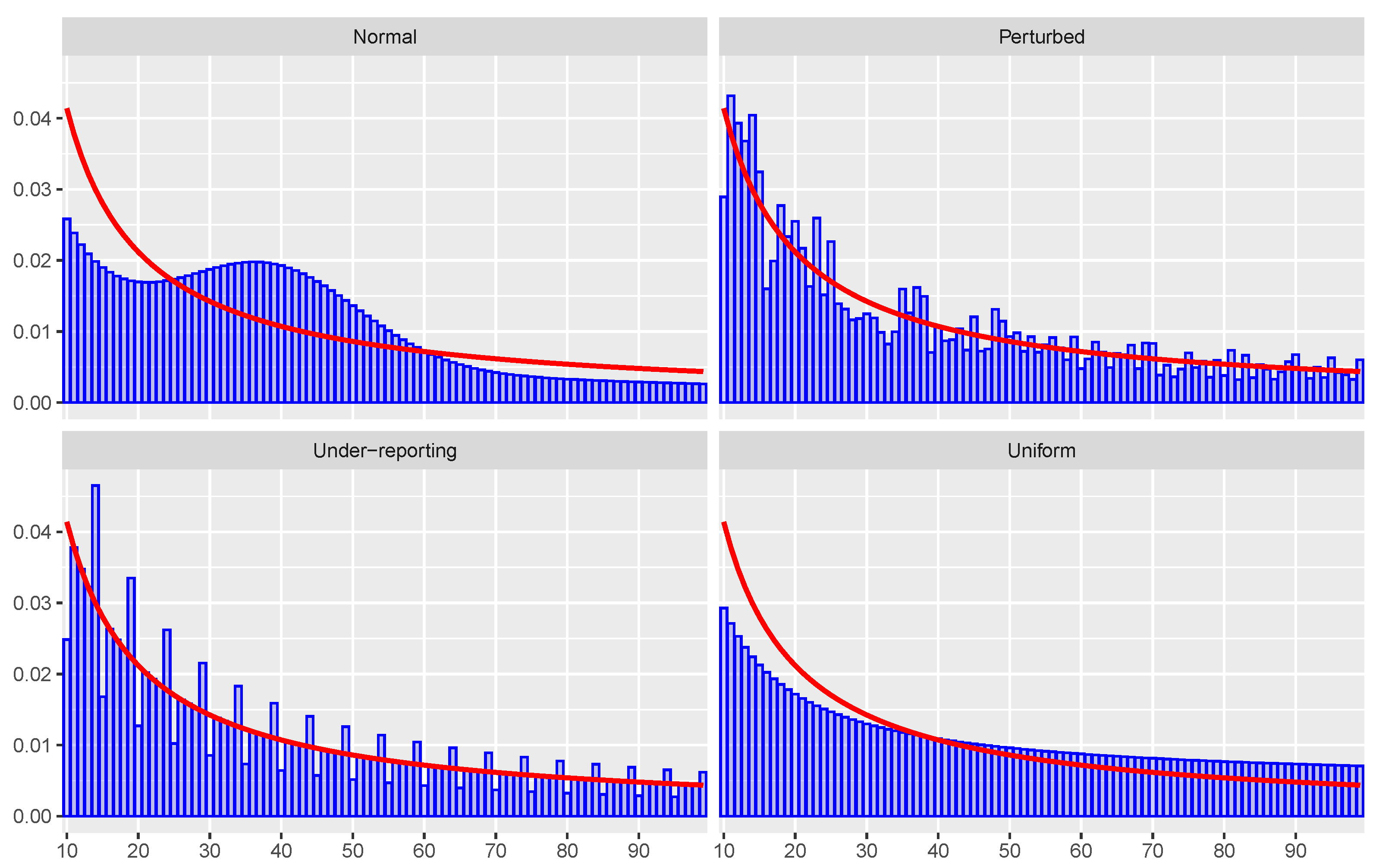
Figure 1. Probability function of the first-two-digits Benford’s law (red) compared to the probability functions of the mixtures used under the alternative hypothesis (blue). In the figure, a mixing parameter λ = 0.6 was used to exaggerate the visual effect. Larger values of λ were used in the simulations, with the consequence that the distribution under the alternative is closer to the distribution under the null.
Stats 04 00044 g001
Figure 2. First digit tests: deviation of the actual size from the nominal size. Tests are as follows: “Adj. MAD”, adjusted MAD (10); “Chi-sq(2)”, χ 2 ( 2 ) test on mean and variance (4); “Chi-sq(d-1)”, χ 2 ( 8 ) test (9); “Mean”, normal test on the mean (1); “Mean & var.”, normal test on mean and variance (3); “Variance”, normal test on variance (2). The number of observations is indicated on top of each panel.
Stats 04 00044 g002
Figure 3. First digit tests: size–power curves of the tests against the uniform mixing alternative with λ = 0.9 . Tests are as follows: “Adj. MAD”, adjusted MAD (10); “Chi-sq(2)”, χ 2 ( 2 ) test on the mean and variance (4); “Chi-sq(d-1)”, χ 2 ( 8 ) test (9); “Mean”, normal test on the mean (1); “Mean & var.”, normal test on mean and variance (3); “Variance”, normal test on variance (2). The dashed line is p o w e r = a c t u a l s i z e . The number of observations is indicated on top of each panel.
Stats 04 00044 g003
Figure 4. First digit tests: size–power curves of the tests against the normal mixing alternative with λ = 0.9 . Tests are as follows: “Adj. MAD”, adjusted MAD (10); “Chi-sq(2)”, χ 2 ( 2 ) test on mean and variance (4); “Chi-sq(d-1)”, χ 2 ( 8 ) test (9); “Mean”, normal test on the mean (1); “Mean & var.”, normal test on mean and variance (3); “Variance”, normal test on variance (2). The dashed line is p o w e r = a c t u a l s i z e . The number of observations is indicated on top of each panel.
Stats 04 00044 g004
Figure 5. First digit tests: size–power curves of the tests against the perturbed mixing alternative with λ = 0.75 . Tests are as follows: “Adj. MAD”, adjusted MAD (10); “Chi-sq(2)”, χ 2 ( 2 ) test on mean and variance (4); “Chi-sq(d-1)”, χ 2 ( 8 ) test (9); “Mean”, normal test on the mean (1); “Mean & var.”, normal test on mean and variance (3); “Variance”, normal test on variance (2). The dashed line is p o w e r = a c t u a l s i z e . The number of observations is indicated on top of each panel.
Stats 04 00044 g005
Figure 6. First two digits tests: deviation of the actual size from the nominal size. Tests are as follows: “Adj. MAD”, adjusted MAD (10); “Chi-sq(2)”, χ 2 ( 2 ) test on mean and variance (4); “Chi-sq(d-1)”, χ 2 ( 89 ) test (9); “Mean”, normal test on the mean (1); “Mean & var.”, normal test on mean and variance (3); “Variance”, normal test on variance (2). The number of observations is indicated on top of each panel.
Stats 04 00044 g006
Figure 7. First two digits tests: size–power curves of the tests against the uniform mixing alternative with λ = 0.9 . Tests are as follows: “Adj. MAD”, adjusted MAD (10); “Chi-sq(2)”, χ 2 ( 2 ) test on mean and variance (4); “Chi-sq(d-1)”, χ 2 ( 89 ) test (9); “Mean”, normal test on the mean (1); “Mean & var.”, normal test on mean and variance (3); “Variance”, normal test on variance (2). The dashed line is p o w e r = a c t u a l s i z e . The number of observations is indicated on top of each panel.
Stats 04 00044 g007
Figure 8. First two digits tests: size–power curves of the tests against the normal mixing alternative with λ = 0.9 . Tests are as follows: “Adj. MAD”, adjusted MAD (10); “Chi-sq(2)”, χ 2 ( 2 ) test on mean and variance (4); “Chi-sq(d-1)”, χ 2 ( 89 ) test (9); “Mean”, normal test on the mean (1); “Mean & var.”, normal test on mean and variance (3); “Variance”, normal test on variance (2). The dashed line is p o w e r = a c t u a l s i z e . The number of observations is indicated on top of each panel.
Stats 04 00044 g008
Figure 9. First two digits tests: size–power curves of the tests against the perturbed mixing alternative with λ = 0.75 . Tests are as follows: “Adj. MAD”, adjusted MAD (10); “Chi-sq(2)”, χ 2 ( 2 ) test on mean and variance (4); “Chi-sq(d-1)”, χ 2 ( 89 ) test (9); “Mean”, normal test on the mean (1); “Mean & var.”, normal test on mean and variance (3); “Variance”, normal test on variance (2). The dashed line is p o w e r = a c t u a l s i z e . The number of observations is indicated on top of each panel.
Stats 04 00044 g009
Figure 10. First two digits tests: size–power curves of the tests against the rounding mixing alternative with λ = 0.75 . Tests are as follows: “Adj. MAD”, adjusted MAD (10); “Chi-sq(2)”, χ 2 ( 2 ) test on mean and variance (4); “Chi-sq(d-1)”, χ 2 ( 89 ) test (9); “Mean”, normal test on the mean (1); “Mean & var.”, normal test on mean and variance (3); “Variance”, normal test on variance (2). The dashed line is p o w e r = a c t u a l s i z e . The number of observations is indicated on top of each panel.
Stats 04 00044 g010
Figure 11. Average estimated M A D s over 1000 replications under the (Benford’s law) null hypothesis (blue points) and α / n (black curve) for varying sample sizes n ( 250 , 500 , , 10 , 000 ) . α is a scale factor used to report 1 / n on the same scale as M A D . The shaded area represents the central 90% of the distribution of estimated M A D s. The horizontal dashed line corresponds to Nigrini’s suggested critical value (0.0022). The vertical dashed line corresponds to n = 1750 .
Stats 04 00044 g011
Figure 12. Behaviour of conformance tests across samples. In the first row (panels AC), data conform to the “first two digits” Benford’s law. In the second row (panels DF), data follow a perturbed Benford’s law with λ = 0.95 . In the third row (panels GI), data are consistent with a perturbed Benford’s law with λ = 0.75 . The first column (panels A,D,G) reports the results computed over the full sample, with n = 15,000. The second column (panels B,E,H) is relative to a single random subsample with n = 1750. The third column (panels C,F,I) reports the estimated densities (blue) of the conventional (or Wald) chi-square test statistic over 5000 random subsamples of length n = 1750 along with the χ 2 ( 89 ) distribution under the null distribution (red). P ( χ 89 2 ) and P ( A d j . M A D ) denote p values of the conventional (or Wald) chi-square test and of the adjusted M A D test, respectively. P r o b . o f s u p . is an estimate of the probability of superiority.
Stats 04 00044 g012
Publisher’s Note: MDPI stays neutral with regard to jurisdictional claims in published maps and institutional affiliations.