First Digit Oscillations

Abstract

The frequency of the first digits of numbers drawn from an exponential probability density oscillate around the Benford frequencies. Analysis, simulations and empirical evidence show that datasets must have at least 10,000 entries for these oscillations to emerge from finite-sample noise. Anecdotal evidence from population data is provided.

1. Introduction

According to Benford’s law, the frequency of the first digits of numbers are larger for digit 1 (about 30%) than 2 (about 18%) and so on up to 9 (about 5%). The “law” that governs these probabilities $b_d$ is

$$b_d={log}_{10}(1+1/d),$$

(1)

where $d=1,2,\dots ,9$. This law originated with Simon Newcomb [1] and was popularized by Frank Benford [2]. In 1995, T. P. Hill [3] proved a theorem that helps explain the success of Benford’s first digit law. According to Hill’s theorem, the frequency of the first digits of numbers randomly drawn from randomly chosen distributions converge to $b_d$ in the limit of large numbers. Several books introduce and summarize findings on the subject [4,5,6].

Benford illustrated Equation (1) with “found” or empirical datasets drawn from a number of sources. Many empirical sets of numbers observe or approximate Benford’s first digit law, particularly those that (1) span several decades; (2) have positive skewness; (3) have many entries; and (4) are not intentionally designed. Such datasets have been called “Benford suitable” by Goodman [7].

Even so, some numerically generated datasets that are Benford suitable do not observe Benford’s law in detail. In particular, consider numbers drawn from an exponential probability density

$$p_{\lambda }\left(t\right)=\lambda exp(-\lambda t),$$

(2)

where $0\le t\le \infty$ and $\lambda$ are the rate or, equivalently, the inverse mean of the exponential probability density given by

$${\lambda }^{-1}={\int }_0^{\infty }t{p}_{\lambda }\left(t\right)dt.$$

(3)

The first digits of numbers drawn from Equation (2) oscillate with $\lambda$ around $b_d$ with amplitudes of about 10%.

Random numbers drawn from the exponential probability density (2) are important because they approximate pieces of a quantity that is randomly partitioned [8]. Suppose, for instance, that a population P is to be divided, without bias, into M cities and towns in such a way that the mean city size $P/M$ is a definite quantity. If this partition is done so as to maximize the entropy of the partition, we find that the probability of city size t is given by (2), where $\lambda =M/P$. See Appendix A for a derivation of this claim that is inspired by a similar derivation by Iafrate, Miller, and Strach [9]. Miller and Nigrini [10] also explore relations between the exponential probability density (2) and Benford’s law (1).

We might expect the oscillations in the exponential probability density (2) with $\lambda$ to have been observed in real-world data. However, our analysis shows that the predicted oscillations emerge from finite-sample noise only with a sample number $N>$ 10,000. We also describe a real-world example of this first digit oscillation in the populations of US towns and cities as they have evolved over the last hundred years.

2. First Digit Probabilities

The probability $g_d\left(\lambda \right)$ that a number drawn from the exponential distribution (2) has a first digit d is given by

$$\begin{array}{ccc}\hfill g_d\left(\lambda \right)& =& \sum _{k=-\infty }^{\infty }{\int }_{d{10}^k}^{(d+1){10}^k}{p}_{\lambda }\left(t\right)dt\hfill \\ & =& \sum _{k=-\infty }^{\infty }[exp(-\lambda d{10}^k)-exp(-\lambda (d+1){10}^k)].\hfill \end{array}$$

(4)

According to Equation (4), the first digit probability $g_d\left(\lambda \right)$ is periodic in $\lambda$ in the sense that $g_d\left(10\lambda \right)=g_d\left(\lambda \right)$. Reference [11], from whose paper the contents of this section originate, demonstrated that the averages of $g_d\left(\lambda \right)$ over one decade of $\lambda$ are the Benford frequencies $b_d$. The $n=0$ and $n=\pm 1$ terms of a Fourier expansion of (4) produce the formula

$$g_d\left(\lambda \right)\approx b_d+(\frac{4r}{ln10})sin[\pi {log}_{10}(1+1/d)]sin[\theta +2\pi {log}_{10}(\lambda \sqrt{d(1+d)})],$$

(5)

where r and $\theta$ are, respectively, the absolute value and argument of the gamma function $\mathsf{\Gamma }(-2\pi i/ln10)$.

The first two factors in the second term on the right hand side of (5) characterize an oscillation amplitude of approximately 10% of the non-oscillating term $b_d$, while the last factor is periodic in ${log}_{10}\left(\lambda \right)$. The $n=\pm 2$ Fourier coefficients are approximately ${10}^{-2}$ times smaller than the $n=\pm 1$ coefficients. Higher order coefficients are even smaller. Indeed, formula (5) produces curves visually identical to those produced by the more complete expression (4).

3. Sample Noise

Because the magnitude of the oscillating term in Equation (5) is approximately 10% of the non-oscillating term $b_d$, its effect can easily be swamped by the noise inherent in finite datasets and finite samples from the exponential probability distribution (2). We see this in the following way.

Assume a list of N identically distributed, statistically independent, random numbers indexed with $j=1,2,\cdots N$. Now let $X_{d,j}$ be an indicator random variable defined so that $X_{d,j}=1$ when the number subscripted j begins with digit d and $X_{d,j}=0$ when the number subscripted j does not begin with digit d. We then define the frequency $G_d$ of the first digit d among N numbers as

$$G_d=\frac{1}{N}\sum _{j=1}^N{X}_{d,j}.$$

(6)

The expectation value of both sides of Equation (6) is

$$\begin{array}{ccc}\hfill E\left[G_d\right]& =& \frac{1}{N}\sum _{j=1}^{N}E\left[X_{d,j}\right]\hfill \\ & =& E\left(X_d\right),\hfill \end{array}$$

(7)

since the $X_{d,j}$ are identically distributed, $E\left[X_{d,1}\right]=E\left[X_{d,2}\right]=\cdots E\left[X_{d,N}\right]$, and, therefore, we may denote each of these terms by $E\left[X_d\right]$. When the numbers determining the indicator random variables $X_{d,j}$ are drawn from an exponential distribution, $E\left[G_d\right]$ and $E\left[X_d\right]$ are equal to $g_d\left(\lambda \right)$.

The variance of $G_d$ is generated from

$$\begin{array}{ccc}\hfill G_d^2& =& \frac{1}{N^2}\sum _{i,j=1}^N{X}_{d,i}{X}_{d,j}\hfill \\ & =& \frac{1}{N^2}\sum _{i=1}^N{X}_{d,i}^2+\frac{1}{N^2}\sum _{i,j=1,i\ne j}^N{X}_{d,i}{X}_{d,j}.\hfill \end{array}$$

(8)

Since the $X_{d,i}$ are statistically independent and identically distributed, the $E(X_{d,i}^2)$ are identical and, therefore, can be denoted by $E\left(X_d^2\right)$. Consequently, we find that

$$E\left(G_d^2\right)=\frac{E\left(X_d^2\right)}{N}+\frac{N(N-1)E{\left(X_d\right)}^2}{N^2}.$$

(9)

Therefore, the variance ${\sigma }_{G_d}^2$ is given by

$$\begin{array}{ccc}\hfill {\sigma }_{G_d}^2& =& E\left(G_d^2\right)-E{\left(G_d\right)}^2\hfill \\ & =& \frac{E\left(X_d^2\right)-E{\left(X_d\right)}^2}{N}.\hfill \end{array}$$

(10)

However, because $X_d$ is an indicator random variable with only two possible values, 0 and 1, $E\left(X_d^2\right)=E\left(X_d\right)$. In this case, the variance (10) becomes

$${\sigma }_{G_d}^2=\frac{E\left(X_d\right)-E{\left(X_d\right)}^2}{N}$$

(11)

and the relative standard deviation becomes

$$\frac{{\sigma }_{G_d}}{E\left(G_d\right)}=\frac{1}{\sqrt{N}}\sqrt{\frac{1}{E\left(X_d\right)}-1}.$$

(12)

Recall that $E\left(G_d\right)=E\left(X_d\right)$ and that the analysis resulting in Equations (11) and (12) applies generally to any distribution with indicator random variable $X_d$ and expectation value $E\left(X_d\right)$. Relations (11) and (12), between variance and mean, are, of course, not new. They also follow from the binomial probability distribution that governs the indicator variables.

Given a Benford probability $b_d$ or Benford probability plus oscillation $g_d\left(\lambda \right)$ and standard deviation ${\sigma }_{G_d}$, Equation (12) tells us how many samples N from a distribution are required to resolve the mean frequency in the presence of finite-sample noise. For instance, in order that the relative standard deviation be small enough for the Benford frequency $b_1$$(=0.301)$ of digit $d=1$ to emerge from noise, say, about $10\%$ of $b_1$, $(1/\sqrt{N})\sqrt{1/{log}_{10}\left(2\right)-1}\le 1/10$, which means that $N\ge 200$. However, if one also wants the oscillation of $g_1\left(\lambda \right)$ around the Benford frequency $b_1$ to emerge from sample noise, another $10\%$ reduction in relative standard deviation is needed. In this case, $(1/\sqrt{N})\sqrt{1/{log}_{10}\left(2\right)-1}\le 1/(10·10)$ or $N\ge$ 20,000. We illustrate these calculations in the next section.

4. Sampling

The cumulative probability of the exponential probability density defined in Equation (2) is

$${\int }_0^{t^{\prime }}\lambda exp(-\lambda t)dt=1-exp(-\lambda t^{\prime }),$$

(13)

and can be replaced by the uniform random variable $U(0,1)$, or, equivalently, by $1-U(0,1)$. Simultaneously, $t^{\prime }$ becomes the random variable T drawn from the exponential probability density (2). Therefore, Equation (13) implies that

$$T=\frac{-lnU(0,1)}{\lambda }.$$

(14)

The first digit random variable frequency $G_d$ as determined from the random variables generated by Equation (14) should reflect the $10\%$ oscillations with period ${log}_{10}\lambda$ as predicted by (5), and so they do, as long as the number of samples N is large enough. For more details concerning sampling consult reference [12].

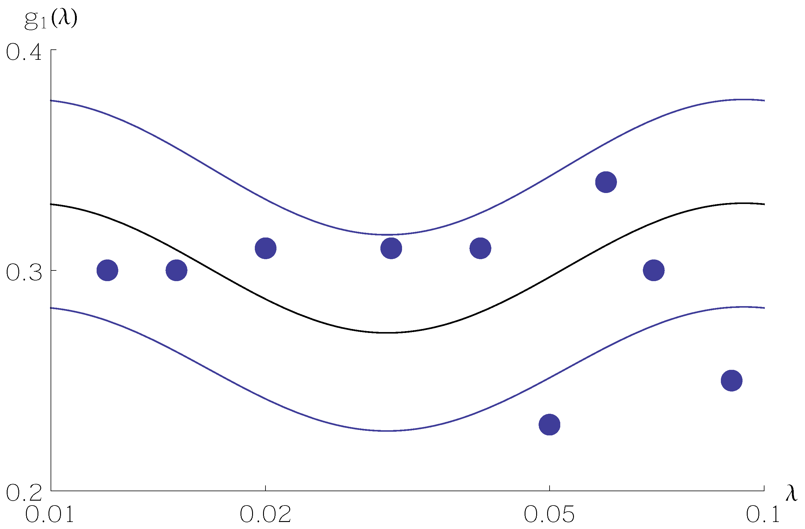
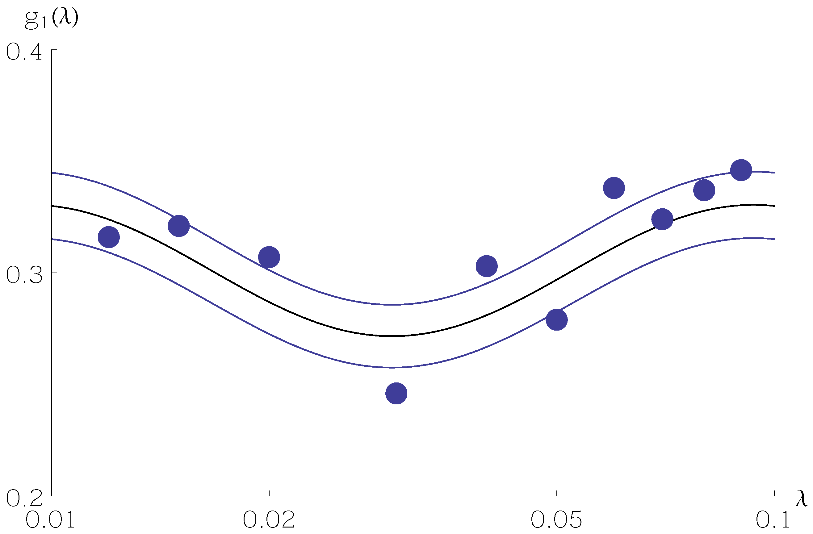
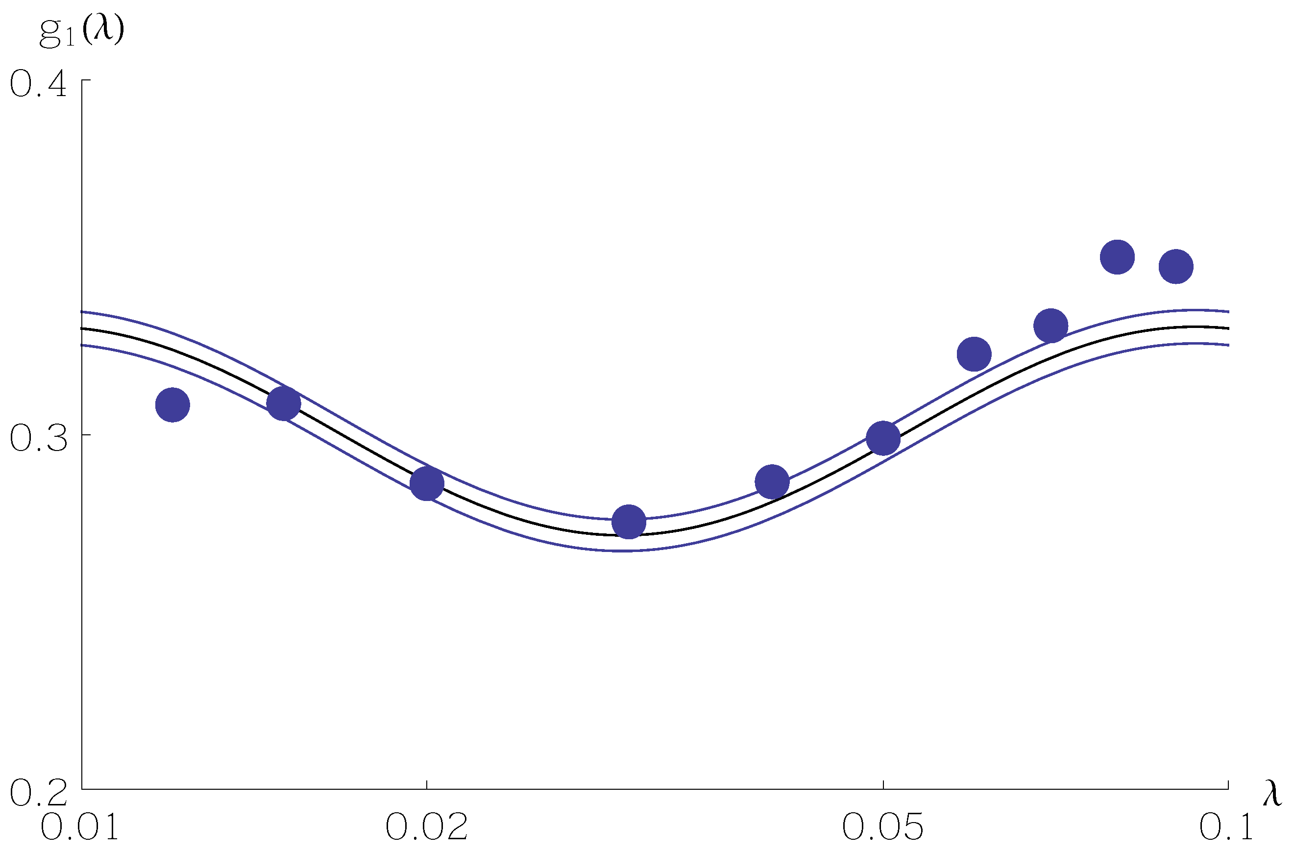
According to (12), the relative standard deviation ${\sigma }_{G_d}/E\left(G_d\right)$ is smallest for a given sample size N when $E\left(X_d\right)$ is largest. For exponentially distributed probabilities this means the oscillation in $\lambda$ will most easily be seen in samples of the random variable $G_1$, that is, when $d=1$. Figure 1, Figure 2 and Figure 3 show sample values of $G_1$ for N$(={10}^2,{10}^3,{10}^4)$ as a function of $\lambda$ between ${10}^{-2}$ and ${10}^{-1}$. Values of the random variable $G_1$ are shown as filled circles. The central curve is $g_1\left(\lambda \right)$ from Equation (5), and the two surrounding curves are $g_1\pm {\sigma }_{G_1}$ from Equation (11) or Equation (12) with $E\left(G_1\right)=E\left(X_1\right)=g_1\left(\lambda \right)$. Values of the random variable $G_1$ mainly stay within the standard deviation curves.

Figure 1. Frequency of first digit 1 versus $\lambda$ from (5) and (11) or (12) with $N=100$. Filled circles are first digit frequencies from $N=100$ samples generated by (14).

Figure 2. Frequency of first digit 1 versus $\lambda$. Curves are from (5) and (11) or (12) with $N=1000$. Filled circles are first digit frequencies from $N=1000$ samples generated by (14).

Figure 3. Frequency of first digit 1 versus $\lambda$. Curves are from (5) and (11) or (12) with $N=$ 10,000. Filled circles are first digit frequencies from $N=$ 10,000 samples generated by (14).

A sample size of $N=100$ hardly allows one to discern the Benford frequency $b_1$ much less the oscillation around $b_1$. Only with larger samples, on the order of $N=$ 10,000, does the $10\%$ oscillation emerge from finite-sample noise.

5. Population of Towns and Cities in the USA

In order to observe the predicted first digit oscillations in real-world data, one must find datasets with more than approximately 10,000 entries and with several different values of the inverse mean $\lambda$. For a first effort, no data seems more likely to reveal these oscillations than that of the US Census Bureau as described in [13]; in particular, the populations of incorporated towns and cities at different 10-year intervals. However, only the decennial censuses from 1970 forward have been digitized. While the population of the USA has increased by $50\%$ since 1970, the number of towns and cities has also increased. For this reason, the inverse mean of the municipal population $\lambda$ has changed very little between 1980 and 2010.

In order to find town and city population data with significantly different inverse means $\lambda$, we reached back to the census of 1910. After making the considerable effort to digitize the 1910 populations of 14,000 incorporated towns and cities as listed in the pdf made available by the US Census Bureau [14], we sorted these numbers (and others from the 1980–2010 period) according to first digits.

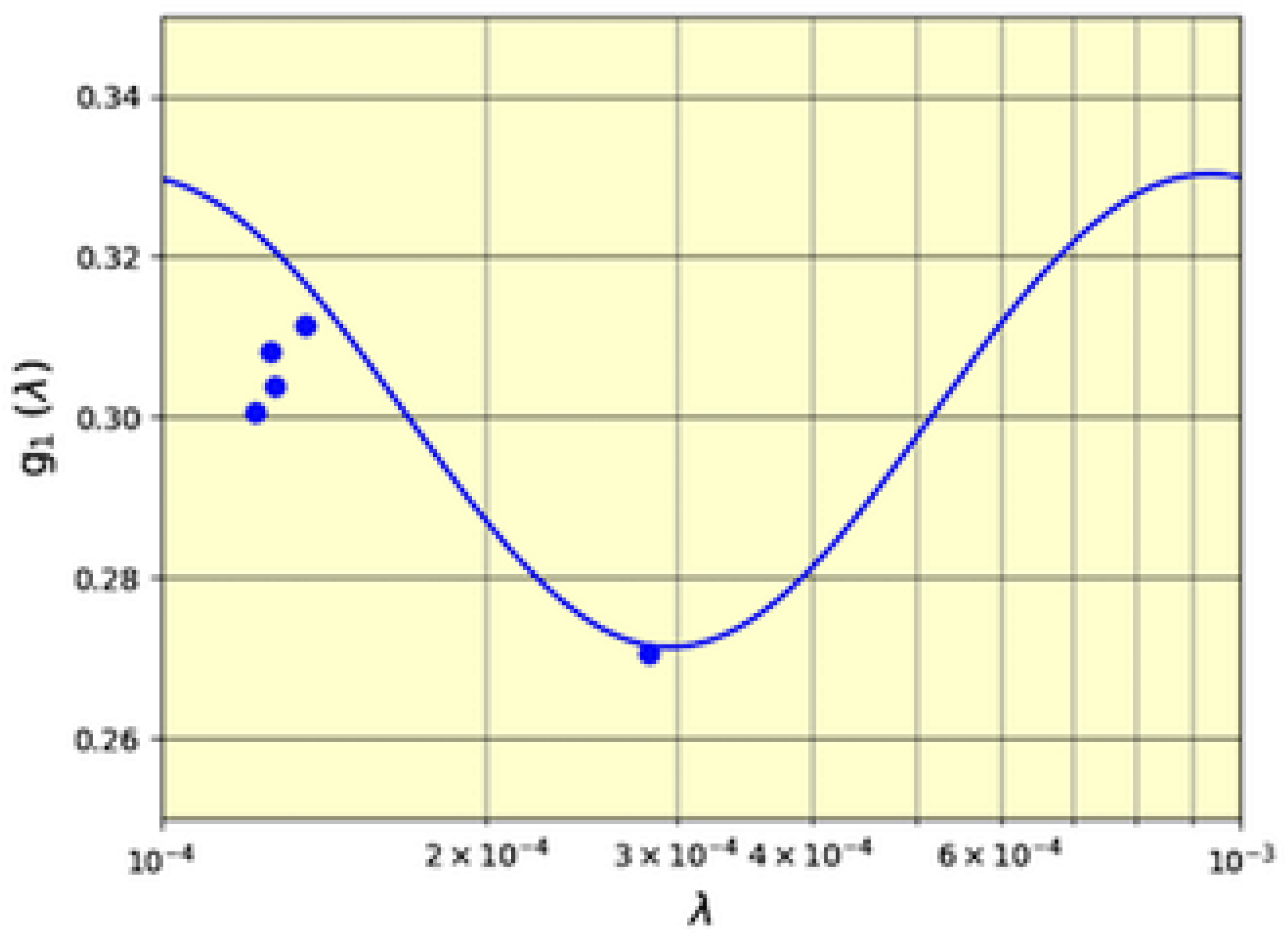
Figure 4 shows the result of our efforts. Here we see the frequency of leading digit 1 for the decennial censuses 1980–2010 (the leftmost group of filled circles) and for 1910 (the rightmost filled circle) versus their respective inverse mean population per town or city $\lambda$. The probability $g_1\left(\lambda \right)$ of first digit 1 as determined by formula (5), which derives from the exponential distribution (2) with parameter $\lambda$, is also shown. Figure 4 does not have standard deviation curves because the number of samples is different for each point.

Figure 4. First digit frequencies versus $\lambda$. Filled circles are frequencies of first digit 1 from the 1980–2010 (leftmost group) and 1910 (rightmost circle) US census. The curve is frequency versus $\lambda$ from formula (5) derived from the exponential probability distribution (2).

Of course, these data merely suggest that the $10\%$ first digit oscillations around Benford frequencies are a feature of population and other real-world data. As such, we hope it encourages others to look for more conclusive evidence. However, as noted, the prerequisite for this search is a Benford suitable dataset with at least 10,000 entries.

6. Summary and Conclusions

In Equation (5), we have made explicit the periodic dependence of the first digit frequencies $g_d\left(\lambda \right)$ of numbers that are drawn from an exponential distribution with rate $\lambda$. According to this relation, the amplitude of these oscillations is approximately $10\%$ of the Benford frequencies $b_d$. We have also demonstrated that the number of data entries required to allow these $10\%$ oscillations to emerge from sample noise in real-world data should be larger than about 10,000. We have illustrated this requirement in numerical realizations of the simulation algorithm in Equation (14). The populations of US towns and cities spanning a century is real-world, if anecdotal, evidence of these first digit oscillations.

While the requirement of 10,000 numbers sets a high bar, sufficiently large Benford suitable datasets do exist and have been sorted according to first digit [15]. The first digit frequencies reported in [15] appear to be consistent with the predicted $10\%$ oscillations around Benford values. However, the appropriate value of $\lambda$, which determines the phase of these oscillations, was not reported.

Alternatively, one might repeat the same experiment many times in which a given quantity is partitioned in such a way that the inverse mean of the partition sizes $\lambda$ is constant. Then, according to the law of large numbers, the mean values of the frequency of first digits will converge to those described by formula (5). Our analysis may explain why those mining specific datasets for evidence of Benford’s law may only fortuitously find agreement within $10\%$ of $b_d$ and then only for certain digits.