fsdaSAS: A Package for Robust Regression for Very Large Datasets Including the Batch Forward Search

Abstract

The forward search (FS) is a general method of robust data fitting that moves smoothly from very robust to maximum likelihood estimation. The regression procedures are included in the MATLAB toolbox FSDA. The work on a SAS version of the FS originates from the need for the analysis of large datasets expressed by law enforcement services operating in the European Union that use our SAS software for detecting data anomalies that may point to fraudulent customs returns. Specific to our SAS implementation, the fsdaSAS package, we describe the approximation used to provide fast analyses of large datasets using an FS which progresses through the inclusion of batches of observations, rather than progressing one observation at a time. We do, however, test for outliers one observation at a time. We demonstrate that our SAS implementation becomes appreciably faster than the MATLAB version as the sample size increases and is also able to analyse larger datasets. The series of fits provided by the FS leads to the adaptive data-dependent choice of maximally efficient robust estimates. This also allows the monitoring of residuals and parameter estimates for fits of differing robustness levels. We mention that our fsdaSAS also applies the idea of monitoring to several robust estimators for regression for a range of values of breakdown point or nominal efficiency, leading to adaptive values for these parameters. We have also provided a variety of plots linked through brushing. Further programmed analyses include the robust transformations of the response in regression. Our package also provides the SAS community with methods of monitoring robust estimators for multivariate data, including multivariate data transformations.

1. Introduction

Data frequently contain outlying observations, which need to be recognised and perhaps modelled. In regression, recognition can be made difficult when the presence of several outliers leads to “masking” in which the outliers are not evident from a least squares fit. Robust methods are therefore necessary. This paper is concerned with the robust regression modelling of large datasets—our major example contains 44,140 univariate observations and five explanatory variables. We use the forward search (FS), which provides a general method of robust data fitting that moves smoothly from very robust to maximum likelihood estimation. Many robust procedures using the FS are included in the MATLAB toolbox FSDA [1,2]. The core of the method is a series of fits to the data for subsets of m observations, with m, incremented in steps of one, going from very small to being equal to n, the total number of observations. As we show in Section 6, the procedure becomes appreciably slower as n increases. The performance of the MATLAB version is further slowed by the language’s handling of large files.

In this paper, we present two enhancements of FS regression for large datasets:

• The Batch Forward Search. Instead of incrementing the subset used in fitting by one observation we move from a subset of size m to one of size $m+k$. In our example, the batch size $k=10$. We use an approximation to test for outliers one observation at a time;
• A SAS version of the program, fsdaSAS (https://github.com/UniprJRC/FSDAsas accessed on 12 March 2021), which takes advantage of the file handling capabilities of SAS to increase the size of datasets that can be analysed and to decrease computation time for large problems.

fsdaSAS, including the option of batches, is one result of a much larger project to provide a SAS version of the FS, which was undertaken in the framework of a European Union program supporting the Customs Union and Anti-Fraud policies. It originates from the need for the analysis of large datasets expressed by law enforcement services operating in the European Union, in particular the EU anti-fraud office. Details of the resulting SAS version of the FS are in the lengthy technical report by Torti et al. [3], which also contains technical documentation on the use of the software. Section 7 of the report emphasises more complex monitoring plots which were not previously available in SAS.

The purposes of the present paper are to introduce a set of SAS programs for robust data analysis, to provide a description of the batch forward search and to illustrate its properties on a previously unanalysed large data example.

The next section provides the basic algebra for the FS, which leads to the calculation of the minimum deletion residuals for the data ordered by closeness to the fitted model. Section 3 describes the properties of the SAS language that make it suitable for handling large datasets and Section 4 illustrates the use of our SAS program FSR.sx in the robust analysis of data on 509 customers at a supermarket in Northern Italy. The batch FS procedure is introduced in Section 5, which describes the approximations used for fast analyses of large datasets. Timing comparisons are in Section 6; Figure 8 shows the considerable advantage of using SAS instead of MATLAB functions for analysing large datasets. The analysis of a large dataset is in Section 7.

The paper concludes with a discussion of more general topics in monitoring robust regression which relates to our SAS routines. The FS for regression, moving through the data and providing a set of fits to increasing numbers of observations, monitors the changes in parameter estimates and residuals due to the introduction of observations into the subset of observations used for estimation. We extended monitoring procedures to several other methods for robust regression. Section 8.1 categorises three methods of robust regression. We provided methods of monitoring hard trimming estimators (LMS and LTS) and soft trimming or downweighting estimators (S and MM). Our SAS programs are listed in Section 8.3. In addition to robust regression, these include routines for robust data transformation, multivariate analysis and model choice.

There are three appendices. The first two provide the algebra of the distributional results for the simultaneous tests of outliers over the search. The third complements our paper with a software survey for robust statistical analyses with our fsdaSAS package.

2. Algebra for the Forward Search

The FS by its nature provides a series of decreasingly robust fits which we monitor for outliers in order to determine how to increment the subset of observations used in the fitting.

Examples and a discussion of monitoring using the MATLAB version of FSDA can be found in Riani et al. [4] and in Appendix C.

The regression model is $y=X\beta +ϵ,$ where y is the $n\times 1$ vector of responses, X is an $n\times p$ full-rank matrix of known constants (with ith row $x_i^{\top }$), and $\beta$ is a vector of p unknown parameters. The independent errors $ϵ$ are normally distributed with mean 0 and variance ${\sigma }^2$.

The least squares estimator of $\beta$ is $\widehat{\beta }$. Then, the vector of n least squares residuals is $e=y-\widehat{y}=y-X\widehat{\beta }=(I-H)y$, where $H=X{\left(X^{\top }X\right)}^{-1}{X}^{\top }$ is the “hat” matrix, with diagonal elements $h_i$ and off-diagonal elements $h_{ij}$. The residual mean square estimator of ${\sigma }^2$ is $s^2=e^{\top }e/(n-p)={\sum }_{i=1}^n{e}_i^2/(n-p).$

The FS fits subsets of observations of size m to the data, with $m_0\le m\le n.$ Let $S^{*}\left(m\right)$ be the subset of size m found by the FS, for which the matrix of regressors is $X\left(m\right)$. Least squares on this subset of observations yields parameter estimates $\widehat{\beta }\left(m\right)$ and $s^2\left(m\right)$, the mean square estimate of ${\sigma }^2$ on $m-p$ degrees of freedom. Residuals can be calculated for all observations including those not in $S^{*}\left(m\right)$. The n resulting least squares residuals are $e_i\left(m\right)=y_i-x_i^{\top }\widehat{\beta }\left(m\right).$ The search moves forward with the augmented subset $S^{*}(m+1)$ consisting of the observations with the $m+1$ smallest absolute values of $e_i\left(m\right)$. In the batch algorithm of Section 5, which is a main topic of this paper, we explore the properties of a faster algorithm in which we move forward by including $k>1$ observations.

To start, we can take $m_0$ as small as $p+1$ and search over subsets of $m_0$ observations to find the subset that yields the LMS estimate of $\beta$. Rules for determining the value of $m_0$ are discussed in Section 4. However, this initial estimator is not important, provided masking is broken. Our computational experience for regression is that randomly selected starting subsets also yield indistinguishable results over the last one third of the search, unless there is a large number of structured outliers.

To test for outliers, the deletion residual is calculated for the $n-m$ observations not in $S^{*}\left(m\right)$. These residuals, which form the maximum likelihood tests for the outlyingness of individual observations, are:

$$r_i\left(m\right)=\frac{y_i-x_i^{\top }\widehat{\beta }\left(m\right)}{\sqrt{s^2\left(m\right)\{1+h_i\left(m\right)\}}}=\frac{e_i\left(m\right)}{\sqrt{s^2\left(m\right)\{1+h_i\left(m\right)\}}},$$

(1)

where the leverage $h_i\left(m\right)=x_i^{\top }{\left\{X{\left(m\right)}^{\top }X\left(m\right)\right\}}^{-1}{x}_i$. Let the observation nearest to those forming $S^{*}\left(m\right)$ be $i_{\mathrm{m}\mathrm{i}\mathrm{n}}$ where:

$$i_{\mathrm{m}\mathrm{i}\mathrm{n}}=arg\underset{i\notin S^{*}\left(m\right)}{min}\left|r_i\left(m\right)\right|.$$

To test whether observation $i_{\mathrm{m}\mathrm{i}\mathrm{n}}$ is an outlier, we use the absolute value of the minimum deletion residual:

$$r_{\mathrm{m}\mathrm{i}\mathrm{n}}\left(m\right)=\frac{e_{\mathrm{i}\mathrm{m}\mathrm{i}\mathrm{n}}\left(m\right)}{\sqrt{s^2\left(m\right)\{1+h_{\mathrm{i}\mathrm{m}\mathrm{i}\mathrm{n}}\left(m\right)\}}},$$

(2)

as a pointwise test statistic. If the absolute value of (2) is too large, the observation $i_{\mathrm{m}\mathrm{i}\mathrm{n}}$ is considered a potential outlier, as well as are all other observations not in $S^{*}\left(m\right)$.

The test statistic (2) is the $(m+1)$st ordered value of the absolute deletion residuals. We can therefore use distributional results to obtain envelopes for our plots. The argument parallels that of Riani et al. [5] where envelopes were required for the Mahalanobis distances arising in applying the FS to multivariate data. The details are in Appendix A. We, however, require a samplewise probability for the false detection of outliers, that is over all values of m in the search which are monitored for outliers. The algorithm in Appendix A is designed to have a samplewise size of 1%.

We need to base the detection of outliers on envelopes from a sample that is small enough to be free of outliers. To use the envelopes in the FS for outlier detection, we accordingly propose a two-stage process. In the first stage, we run a search on the data, monitoring the bounds for all n observations until we obtain a “signal” indicating that observation $m^{†}$, and therefore succeeding observations, may be outliers, because the value of the statistic lies beyond our simultaneous threshold. In the second part, we superimpose envelopes for values of n from this point until the first time we introduce an observation that we recognise as an outlier. In our definition of the detection rule, we use the nomenclature $r_{\mathrm{m}\mathrm{i}\mathrm{n}}(m,n^{*})$ to denote that we are comparing the value of $r_{\mathrm{m}\mathrm{i}\mathrm{n}}\left(m\right)$ with envelopes from a sample of size $n^{*}$. With an informative signal, we start superimposing $99\%$ envelopes taking $n^{*}=m^{†}-1,m^{†},m^{†}+1,\dots$ until an outlier is indicated by the rule in Appendix B. Let this value be $m^{+}$. We then obtain the best parameter estimates by using the sample size of $m^{+}-1$. The automatic use of $m=m^{+}-1$ is programmed in our SAS routines.

In the batch FS procedure introduced in Section 5, the search moves in steps of $m+k(k>1)$ rather than in steps of 1. Testing for outliers then uses the approximation to the ordered deletion residuals based on the estimated parameters from a set of m observations to order the next k deletion residuals to be tested as outliers.

3. Why SAS?

SAS is widely used by large commercial and public organisations, such as customs and national tax agencies as well as banking and insurance companies, for its ability to handle large datasets and relatively complicated calculations. The use of SAS obviates the need for powerful dedicated workstations to perform intensive calculations. Our programs thus make computationally intensive robust statistical analyses available in environments where it would otherwise be economically infeasible. Unfortunately, compared with the R environment and with MATLAB open toolboxes, the standard SAS distribution is lacking in robust methods for data analysis. These issues are discussed in detail in Section 7 of the work by Torti et al. [3].

As an example, the FS monitors the properties of the fitted model over a series of subsets of increasing size. The FSDA package also includes methods for monitoring the fits of other methods of robust regression: for hard trimming, the number of trimmed observations can be varied from approximately $n/2$ to n whereas, for M-estimation, the properties of the fitted model can be monitored for a set of values of asymptotic efficiency or breakdown point. Often monitoring is of various forms of residuals, but score tests are monitored for the Box–Cox transformation and its extensions [6]. Our package provides the SAS community with methods of monitoring regression estimators and their multivariate counterparts, as in the MATLAB FSDA, and also a full set of methods for the FS. Further details of methods of robust regression, as well as of monitoring, are in Section 8.

The idea of monitoring an estimator for various values of its key parameters has shown great potential in data analysis, but the method can be time and space consuming, as the statistics of interest have to be computed and stored many times. This is particularly true for the FS that, for monitoring statistics at each subset size, requires approximately $n^2$ elements to store regression residuals or Mahalanobis distances for a dataset of size n. This means, for example, that almost 1 gigabyte of RAM would be necessary to store a structure for $n=$ 11,000 observations (each numeric variable typically requires 8 bytes). SAS is known for its superior capacity in treating such large datasets. There are several ingredients behind this capacity improvement:

• When the data are at the limit of the physical memory, caching strategies become crucial to avoid the deterioration of performance. Unlike other statistical environments that only run in memory and crash when a dataset is too large to be loaded, SAS uses file-swapping to handle out-of-memory problems. The swapping is very efficient, as the SAS procedures are optimised to limit the number of files created within a procedure, avoiding unnecessary swapping steps;
• File records are stored sequentially, in such a way that processing happens one record at a time. Then, the SAS data step reads through the data only one time and applies all the commands to each line of data of interest. In this way, the data movements are drastically limited and the processing time is reduced;
• A data step only reads the data that it needs in the memory and leaves out the data that it does not need in the source;
• Furthermore, data are indexed to allow for faster retrieval from datasets;
• Finally, in regression and other predictive modelling methods, multi-threading is applied whenever this is appropriate for the analysis.

These good nominal properties seem confirmed by the computing time assessments presented in the next section, showing that our SAS implementation of robust regression tools outperforms the MATLAB counterpart for datasets with more than 1000 units (see Figure 8). We used a separate package based on the IML language (SAS/IML Studio) to realise in SAS a number of FSDA functions requiring advanced graphical output and interactivity. See Section 8 for a summary.

4. FS Analysis of the Transformed Loyalty Card Data

The example in this section serves to illustrate the SAS version of the FS with a set of data sufficiently small not to require the batch search. The data [7] are 509 observations on the behaviour of customers with loyalty cards from a supermarket chain in Northern Italy. The data are themselves a random sample from a larger database. The sample of 509 observations is part of the FSDA toolbox for MATLAB. The response is the amount, in euros, spent at the shop over six months and the explanatory variables are: $x_1$, the number of visits to the supermarket in the six-month period; $x_2$, the age of the customer and, $x_3$, the number of members of the customer’s family. The data are loaded in SAS IML with the commands reported in Figure 1.

Atkinson and Riani [7] show that the Box–Cox transformation can achieve approximate normality for the response and Perrotta et al. [1] recommend a value of 0.4 for the transformation parameter $\lambda$. We work with this value throughout this section.

The starting point of the FS can be set by specifying initial_obs_input as a vector of integers taking values in $[1,n]$, which specify the position of the units to be included in the subset. The length $m_0$ of this vector should be at least $p+1$. If initial_obs_input is not specified, a starting vector of size $p+1$ is estimated using LMS.

The tests described in Equations (1) and (2) start at step $m=\mathtt{i}\mathtt{n}\mathtt{i}\mathtt{t}$. The default value for init is:

$$\mathtt{init}=\left\{\begin{array}{cc}p+1& (n<40)\\ min[3*p+1,\mathrm{floor}\{0.5*(n+p+1)\left\}\right]& (n\ge 40).\end{array}\right.$$

(3)

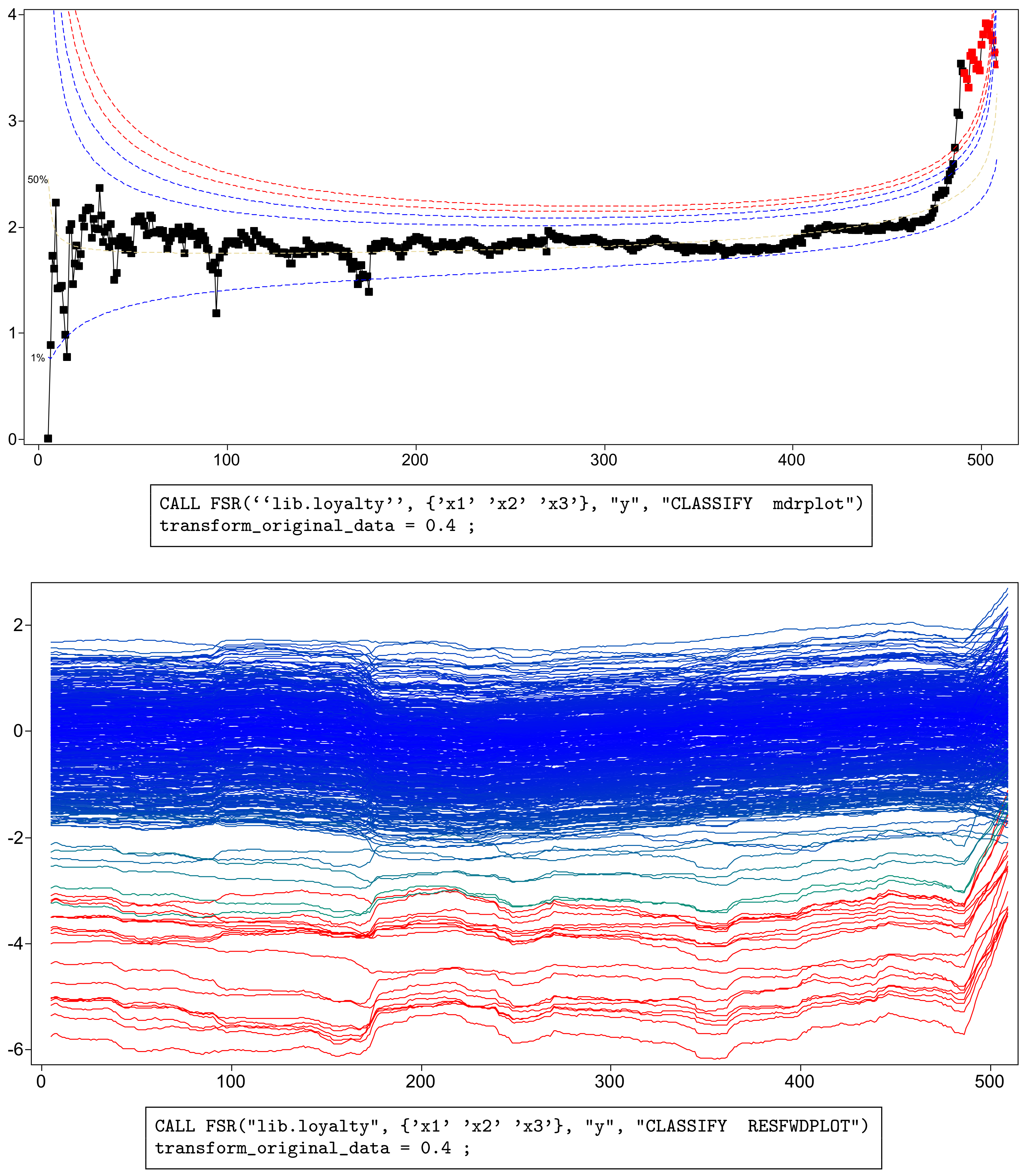
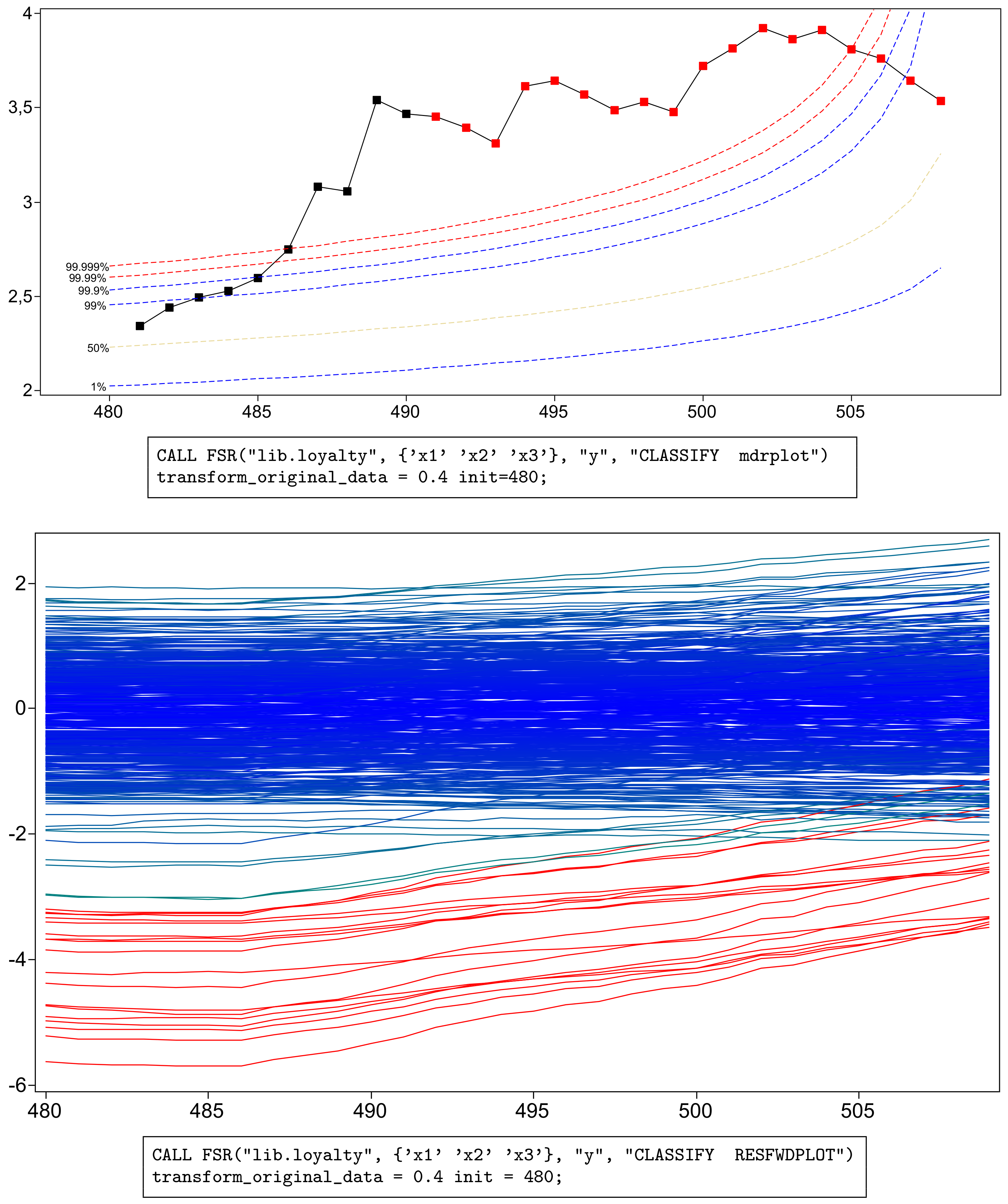
Figure 2 shows, in the top panel, a forward plot of absolute minimum deletion residuals for observations not in the subset used in fitting. Figure 3 shows a zoom of this plot, starting from $m=480$. In addition to the residuals, the plot includes a series of pointwise percentage levels for the residuals (at 1%, 50%, 99%. 99.9%, 99.99% and 99.999%) found by the order statistic arguments of Appendix A. Several large residuals occur towards the end of the search. These are identified by the automatic procedure including the resuperimposition of envelopes described in Appendix B. In all, 18 outliers (plotted as red squares in the online .pdf version) are identified. These form the last observations to enter the subset in the search. The upper panels of the figures, especially Figure 3, show that, at the very end of the search, the trajectory of residuals returns inside the envelopes, the result of masking. As a consequence, the outliers would not be detected by the deletion of single observations from the fit to all n observations. Because of the aspect ratio of the plot, the dramatic decrease in the absolute values of the scaled residuals is less evident in the lower panel of Figure 3 than in that of Figure 2. Both panels show, not only the effect of masking, but also that of “swamping”, in which non-outlying observations are made to appear as outliers towards the end of the search, due to the inclusion of outlying observations in the subset used for parameter estimation.

The plots in Figure 2, Figure 3, Figure 4 and Figure 5 were produced by brushing, i.e., selecting the observations of interest from the top panel of Figure 2 and highlighting them in all others. The bottom panels of the two figures show that the values of the scaled residuals are very stable until the outliers enter and that the outliers all have negative residuals.

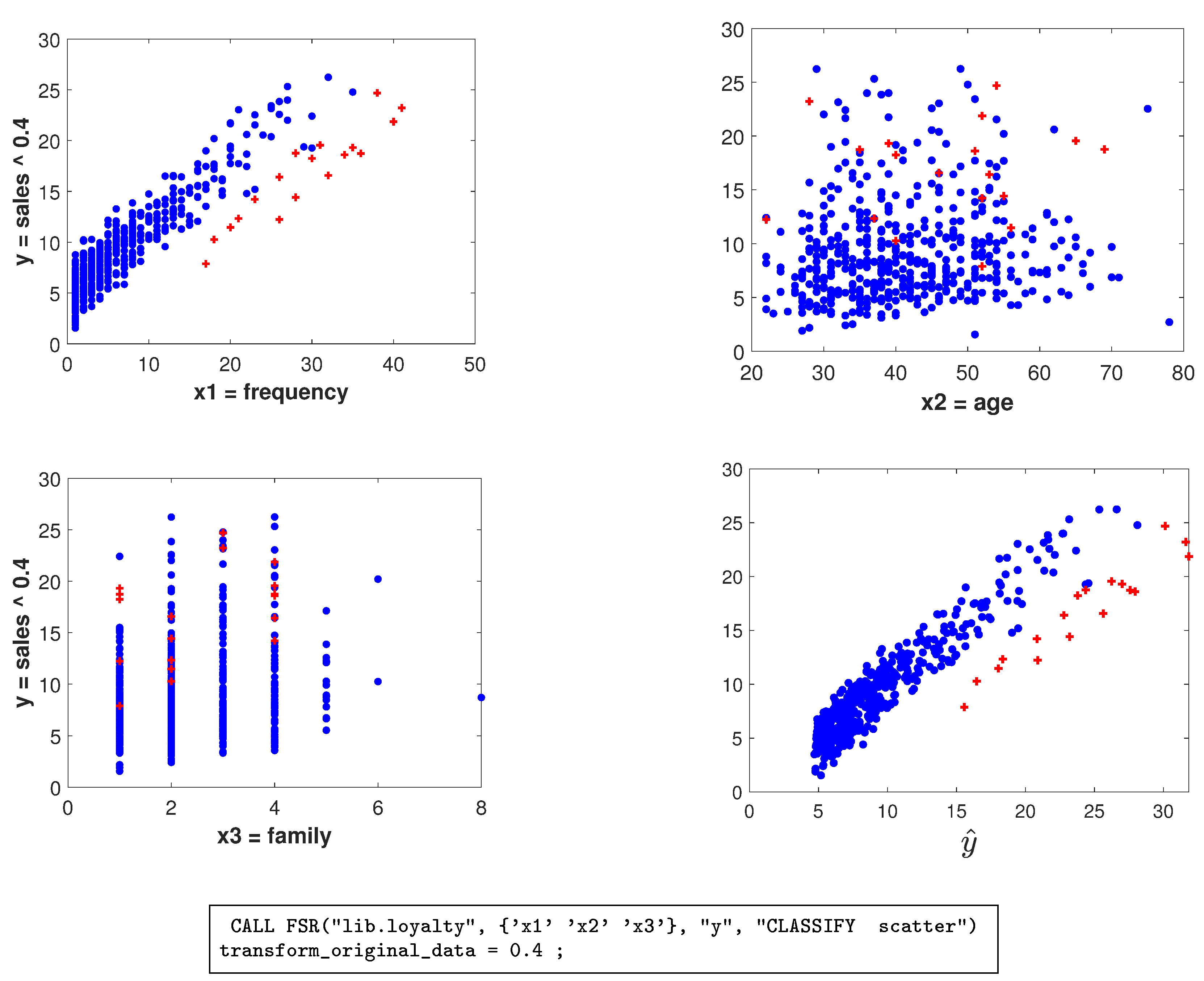
The observations we found are outlying in an interesting way, especially for the values of $x_1$. Figure 4 shows the scatterplots of y against the three explanatory variables, with brushing used to highlight the outlying observations in red (in the online .pdf version). The first panel is of y against $x_1$. The FS identified a subset of individuals, most of whom are behaving in a strikingly different way from the majority of the population. They appear to form a group who spends less than would be expected from the frequency of their visits. This is an example where it might be worth following the suggestion in the first sentence of this paper and finding a model for this identified subset of observations. The scatterplots for $x_2$ and $x_3$, on the other hand, do not show any distinct pattern of outliers. In the last panel, we present a plot, suggested by one referee, of the fitted values on the horizontal axis and the response on the vertical axis. This plot shows a slightly clearer separation of outliers than the plot of response against $x_1$ in the first panel. In the general case, where outlyingness may depend upon several explanatory variables, this plot may carry much more information than scatter plots against individual explanatory variables.

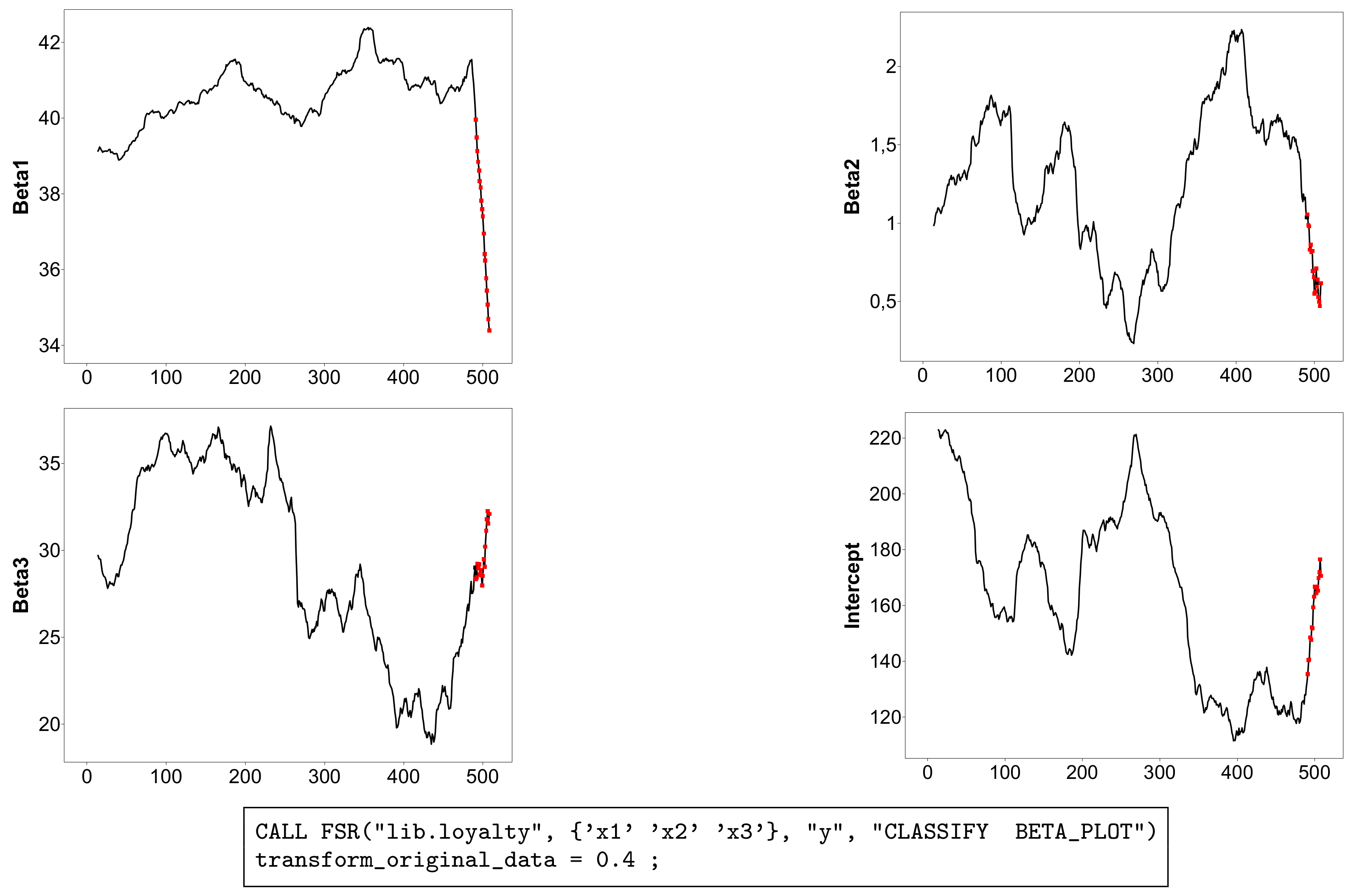
The effect of the 18 outliers on inference can be seen in Figure 5, which gives the forward plots of the four parameter estimates, again with brushing used to plot the outlying observations in red (in the online .pdf version). The upper left panel, for ${\widehat{\beta }}_1$, is the most dramatic. As the outliers are introduced, the estimate decreases rapidly in a seemingly linear manner. This behaviour reflects the position of the outliers in Figure 4, all of which lie below the general linear structure: their inclusion causes ${\widehat{\beta }}_1$ to decrease. The outliers also have effects on the other three parameter estimates (the lower right panel is for the estimate of the intercept ${\beta }_0$). Although the effects for these three parameters are appreciable, they do not take any of the estimates outside the range of values which was found before the inclusion of outliers. The group of outlying customers, who are spending less than would be expected, which does not agree with the model for the majority of the data, will be important in any further modelling.

A SAS analysis using our FS routines that confirms this transformation is in Section 10 of Torti et al. [3]. The robust procedure monitors the approximate score statistic for the transformation parameter introduced by Atkinson [8] and incorporated in the FS by Riani and Atkinson [9]. Distributional results can be found in Atkinson and Riani [10]. The MATLAB version of FS for the extended Yeo–Johnson transformation, in which the responses may be either positive or negative, is described by Atkinson et al. [6].

The left-hand panel of Figure 4 suggests that the outliers might be modelled separately. Another example in which outliers can be distinctly modelled is in data on fraud in seafood pricing, in which the FS analysis of Atkinson et al. [11] shows that the price of imports from one country into the European Union is consistently under reported, leading to tax evasion. The evidence for the existence of this fraud is strengthened by fitting a separate model to the subset of observations.

5. The FS Batch Procedure

Our fsdaSAS contains a new FS strategy that increases the possibility of treating large datasets. The idea is to reduce the size of the output tables and the amount of memory required through a batch updating procedure.

The standard FS algorithm in Section 2 produces a sequence of $n-m_0$ subsets with the corresponding model parameters and relevant test statistics, typically used to test the presence of outliers. The initial subset size $m_0$ can be as small as $p+1$, the minimum number of observations necessary to provide a fit to the data. In the standard algorithm, the subset size $m_0\le m\le n$ is increased by one unit at a time and only the minimum value of the test statistics among the observations outside the subset is retained.

The batch version of the algorithm instead fits to a subset every at $k>1$ steps. The value of k is set by the user through the input parameter fs_steps. The computational time depends on k, the dimension $m_0$ of the initial subset (by default $p+1$), and on the value of m at which testing for outliers starts, determined by the input parameter init, given by (3). The effect of the batches is to decrease computational time, with a slight loss in the accuracy of parameter estimation when outliers are present. To be clear, our procedure is distinct from the batch FS introduced by Cerioli and Riani [12] in the analysis of spatial data. Their batches of neighbouring observations provided parameter estimates for determining the order of the inclusion of subsets in the FS.

Let ${\mathcal{M}}_b$ be the set of values $m_b$ of m at which the model is fitted, with cardinality $n_b$. The search starts with $m=m_0$, so that ${\mathcal{M}}_b=[m_0,m_0+k,m_0+2k,\dots ,n-1].$ For each subset of size $m_b\in {\mathcal{M}}_b$, the search sequentially calculates the estimate $\widehat{\beta }\left(m_b\right)$ and orders the $n-m_b$ deletion residuals for the observations not in the subset. The k smallest values of these test statistics define a subset $S^b\left(m_k\right)$ of k observations. For $m_b<\mathtt{init}$, $m_b$ is augmented by the k data points $S^b\left(m_k\right)$, and a new estimate of $\beta$ is found and the search continues. However, if $m_b\ge \mathtt{init}$, the data points in $S^b\left(m_k\right)$ are assigned in order of ascending values of absolute deletion residual to the succeeding k steps in order to obtain a complete vector of minimum test statistics (2) to be compared with the envelopes. These k statistics are based on the estimate $\widehat{\beta }\left(m_b\right)$. If there is no signal in the search, the subset $m_b$ is, as before, augmented by the k units of $S^b\left(m_k\right)$ and the model is refitted. If there is a signal at unit $k^{*}\in S^b\left(m_k\right)$, we have a signal at the step corresponding to the subset size $m^{†}=m_k+k^{*}$. We now leave the batch search and use the resuperimposition procedure of Section 2 to calculate envelopes for outlier detection, moving forward one observation at a time.

If the effect of re-estimation and resuperimposition is ignored, the number of estimates $\widehat{\beta }\left(m_b\right)$ in the batch FS is at most $n_b=\mathrm{roof}[(n-m_0)/k]$, but may be less if the search terminates early due to an indication of the presence of outliers. The number of tests for outliers is $n-\mathtt{init}-1$. For a large n, this will usually be approximately $n/2$, depending on the value chosen for init. Although the number of estimates is reduced, we have an $mdr$ vector of length between $n/2$ and n and also a matrix of test statistics of dimension $w\times (n-m_0)$ for all the w quantiles of the envelopes; the signal detection phase of the algorithm is identical to the standard FS one. Of course, this vector is an approximation to that which would be found by evaluating each of the k steps individually. The approximation reduces the number of fits to at most $n_b$ while still applying the signal detection, envelope superimposition and signal validation phases described in Appendix B at each of the $n-\mathtt{init}-1$ FS steps. Finally, we note that the time required by the standard FS also depends on the values of $m_0$ and init. The saving in the batch FS comes from a reduced number of steps for parameter estimation and ordering of the deletion residuals. We now examine the gains and losses of the procedure.

If the data are contaminated and k is too large, the approach may not be accurate enough to detect the outliers, giving rise to biased estimates. The problem can be investigated by monitoring the statistical properties of the batch algorithm for increasing k. We conducted such an exploratory assessment using artificial data.

We generated the data using MixSim [13] in the MATLAB implementation of the FSDA toolbox ([14], Section 3); the functions used were MixSimreg.m and simdataset.m. MixSim allows the generation of data from a mixture of linear models on the basis of an average overlap measure $\overline{\omega }$ pre-specified by the user. We generated a dominant linear component containing $95\%$ of the data (blue dots in Figure 6) and a 5% “contaminating” one (black stars) with a small average overlap ($\overline{\omega }=0.01$). The generating regression model is without intercept, with two random slopes from a uniform distribution between $tan\left(\frac{\pi }{6}\right)=\frac{\sqrt{3}}{3}$ and $tan\left(\frac{\pi }{3}\right)=\sqrt{3}$, and independent variables from a uniform distribution in the interval $[0,1]$. Each slope is equally likely to be that of the dominant component. We took the error variances in the two components to be equal when the specification of the value of $\overline{\omega }$, together with the values of the slopes, defines the error variance for each sample. We also added the additional uniform contamination of $3\%$ of the above data (red crosses) over the rectangle defined by the ranges of the dependent and independent variables. The plots in Figure 6 are examples of two datasets with $4750+250+150$ units.

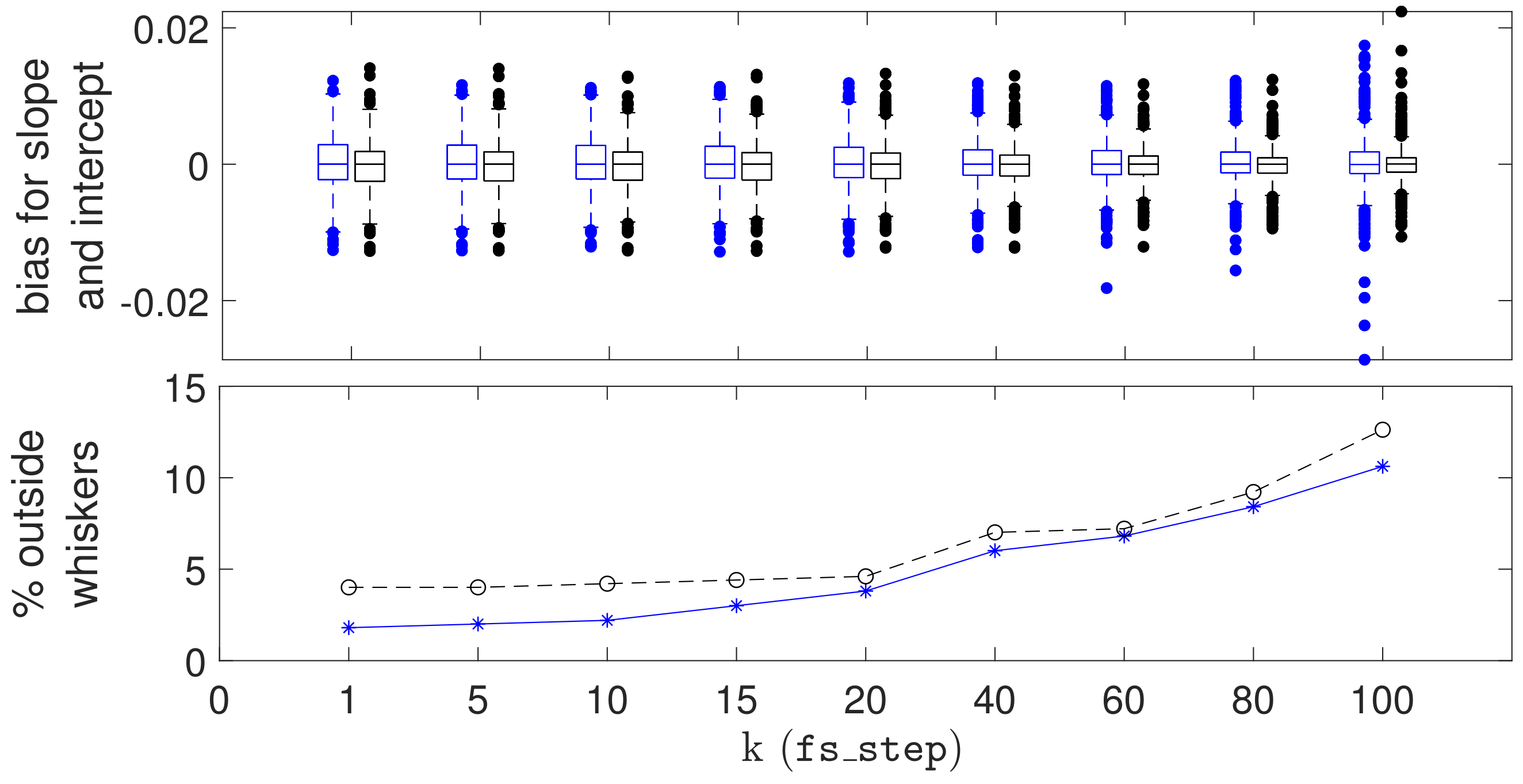
The boxplots of Figure 7 show the bias for the slope and intercept obtained from 500 such datasets with 5150 observations each, for $k\in \{1,5,10,15,20,40,60,80,100\}$. The bias here is simply the difference between the estimated and real slopes, the latter referring to the dominant generating component.

The upper panel of the figure shows that the median bias for both the slopes and intercepts are virtually zero. The dispersion of the estimates for the slopes and intercept remain both stable and quite small even for values of k approaching 100 (note that the boxplot whiskers are in $[-0.01,0.01]$). However, the variability of the estimates outside the whiskers rapidly increases as k approaches 100. The fact that the bottom and top edges of the boxes seem to become smaller for increasing k may be interpreted as a reduced capacity of the batch FS to capture the fine grained structure of the data when k is too large.

The stability of the batch procedure can also be appreciated by looking, in the bottom panel of the figure, at the number of estimated slope and intercept parameters outside the boxplot whiskers: up to $k=10$, there is no appreciable increase with respect to the standard FS with $k=1$; between $k=10$ and $k=20$, the increase is still contained to 5%; then, the number of poor estimates rapidly increases to exceed $10\%$. Finally, there is no evidence of major failure of the batch FS to reject outliers, which would be shown by occasional very large values of bias.

6. Timing Comparisons

We now describe the results of an assessment of the computational benefit of the new batch FS approach available only in SAS, in comparison with the standard SAS and FSDA MATLAB implementations. We tested the functions on a workstation with a CPU 2 x Xeon E5-262v4 (2.6GHz 4cores), two 32 GB DDR4 2400 ECC RAMs, and a Disk SSD of 512GB, equipped with MATLAB R2020a and SAS 9.4.

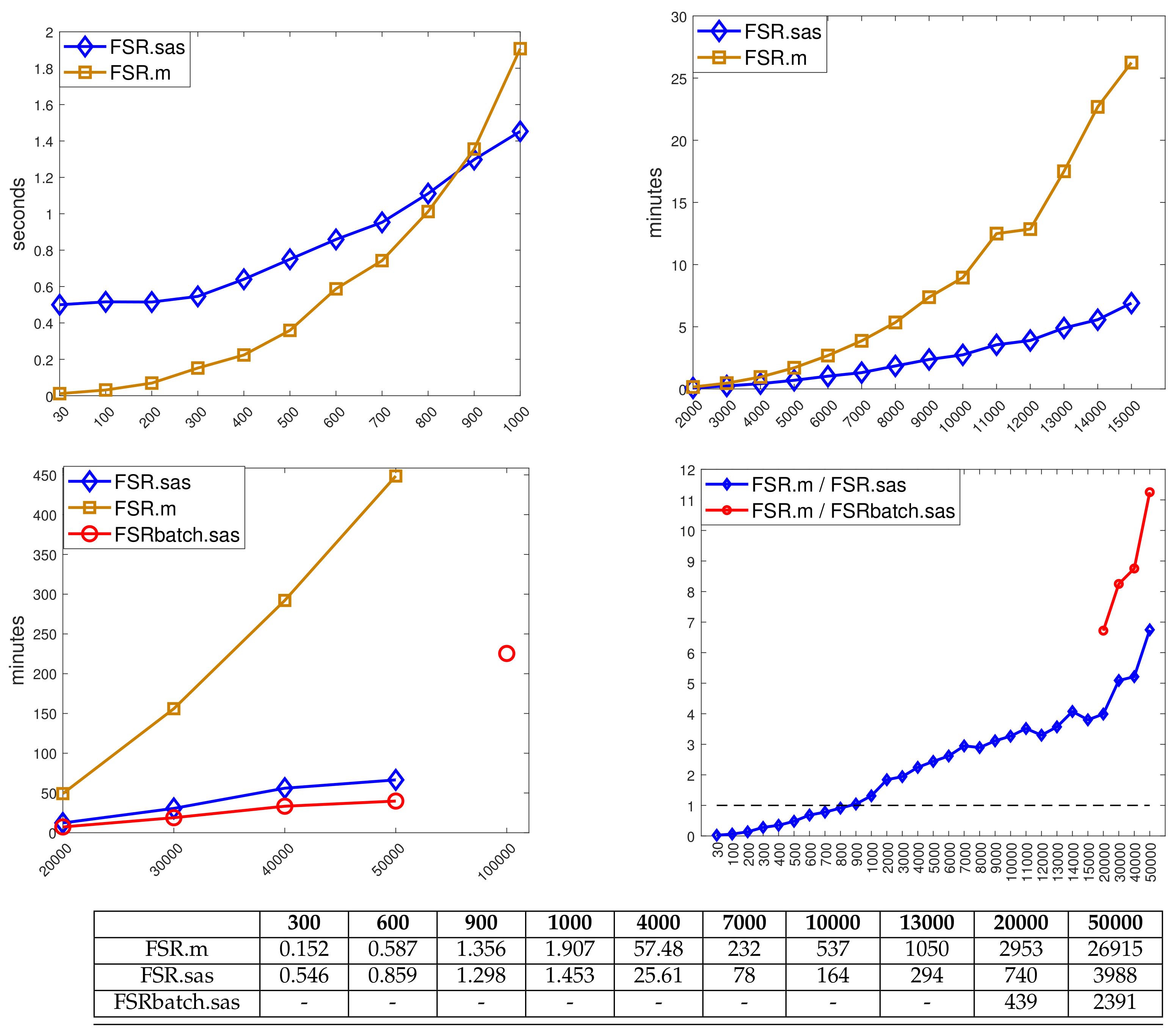
Figure 8 shows the elapsed time needed for analysing the simulated datasets of different sizes (from 30 to 100,000), when fitting one explanatory variable. The results are split into three panels for small ($n=30,\dots$, 1000), medium ($n=$2000, …, 15,000) and large data sizes ($n=$ 20,000,…, 100,000). The bottom-right panel gives the ratio between the time required by the MATLAB implementation and the two SAS ones. For small samples, the FSDA MATLAB implementation (orange squares) is faster than the standard SAS implementation (blue diamonds), but there is a crossing point at a sample size between $n=800$ and $n=900$ where the latter starts to perform better. The advantage of using the SAS function increases for larger sample sizes. For example, in a sample of 50,000 observations SAS was about 7 times faster. The batch option in SAS (red circles), with $k=10$, is even faster: 12 times faster in a sample of 50,000 observations; note that in Figure 8, the batch results are reported only for $n\ge$ 20,000. For smaller values, the reduction in computation time is unlikely to be important, even though Figure 7 shows that for $k=10$ there is a negligible increase in the variability of the parameter estimates from the use of the batch procedure.

The bottom-left panel shows that the standard SAS and FSDA MATLAB implementations crash (because of memory limits) when the sample sizes exceed 50,000 observations. Only the SAS batch algorithm seems to cope with larger datasets ($n=$ 100,000 in the figure), which however, requires about 3.5 h to terminate.

Finally, by interpolating the time values in the three cases with a quadratic curve—the time complexity for producing n statistics for n steps is expected to be $\mathcal{O}\left(n^2\right)$—we found the following approximate coefficients for the quadratic terms: $1.23\times {10}^{-5}$ for the MATLAB implementation, $1.98\times {10}^{-6}$ for the SAS standard implementation, $7.17\times {10}^{-7}$ for the SAS batch implementation (the last one fitted on all n values, not reported in the Figure). This ranking might be used to extrapolate the computational performances of the three FSR implementations for n values not considered here, on hardware configurations that can cope with larger data structures.

7. Balance Sheet Data—A Large Dataset

We now compare the results of the FS analyses of a large dataset with and without the use of batches. The data come from balance sheet information on limited liability companies in Italy. The variables are:

y	profitability, calculated as return over sales;
$x_1$	labour share; the ratio of labour cost to value added;
$x_2$	the ratio of tangible fixed assets to value added;
$x_3$	the ratio of intangible assets to total assets;
$x_4$	the ratio of industrial equipment to total assets;
$x_5$	the firm’s interest burden; the ratio of the firm’s total assets to net capital.

There are 44,140 observations derived from a larger set; observations with zero values of any of the explanatory variables have been omitted, as have the few with negative responses. Corbellini et al. [15] studied the labour share in a related dataset of more than thirty thousand firms over a time span of ten years using robust multivariate regression techniques and the monotonic version of the ACE transformation [16] allowing the transformation of both positive and negative responses. Atkinson et al. [6] analysed a subset of 1405 observations including 407 with negative responses, to illustrate the properties of the extended Yeo–Johnson transformation which is a combination of two Box–Cox transformations. For the positive observations, they found the square root transformation, which we also use in our analysis.

The aim of the data analysis was to explain the profitability by regression on the five explanatory variables. The forward plot of the minimum deletion residuals from both searches is similar in form to Figure 2, but with less extreme outliers at the end of the search; 145 outliers are detected with the standard FS, 161 with the batch FS with $k=10$.

The effect of the 161 outliers on inference can be seen in

Table 1. Balance sheet data: summary properties of regression for least squares computed on all data (column 2), for a standard FS (column 3) and SAS batch with $k=10$ (column 4).

	Least Squares on All Data	Standard FS	Batch FS $\mathit{k}=10$
Number of units	44,140	43,995	43,979
Error d.f. $\nu$	44,134	43,989	43,973
$t_{\nu }$ values
Intercept	377.0	383.5	383.9
$x_1$	−249.3	−253.9	−254.2
$x_2$	−47.4	−48.5	−48.5
$x_3$	−10.2	−10.4	−10.3
$x_4$	−5.0	−4.9	−5.0
$x_5$	−15.2	−15.5	−15.5
$F_{5,\nu }$ for regression $\times {10}^4$	1.274	1.322	1.325
$R^2$	0.591	0.601	0.600

which presents the values of the t-statistics for the six parameters of the model arising from the three different fits. Column 2 of the table shows the least squares results for the full data and the third column the MATLAB FSDA results. In going from the second to the third column the 145 observations identified as outliers have been deleted. As a result, all t-statistics increase in value (apart from a slight decrease in that for $x_4$). There are also increases in the F statistic for regression and in the values of $R^2$. Deleting the outliers has made it possible to extract more information from the data. In going from the third column to the fourth, a further 16 observations have been deleted, which were labelled as outliers by the batch search which also found the 145 outliers determined by FSDA. The effect on the statistics in Table 1 is a small further improvement in four out of seven statistics. These changes are practically negligible, as might be excepted with such a large set of data.

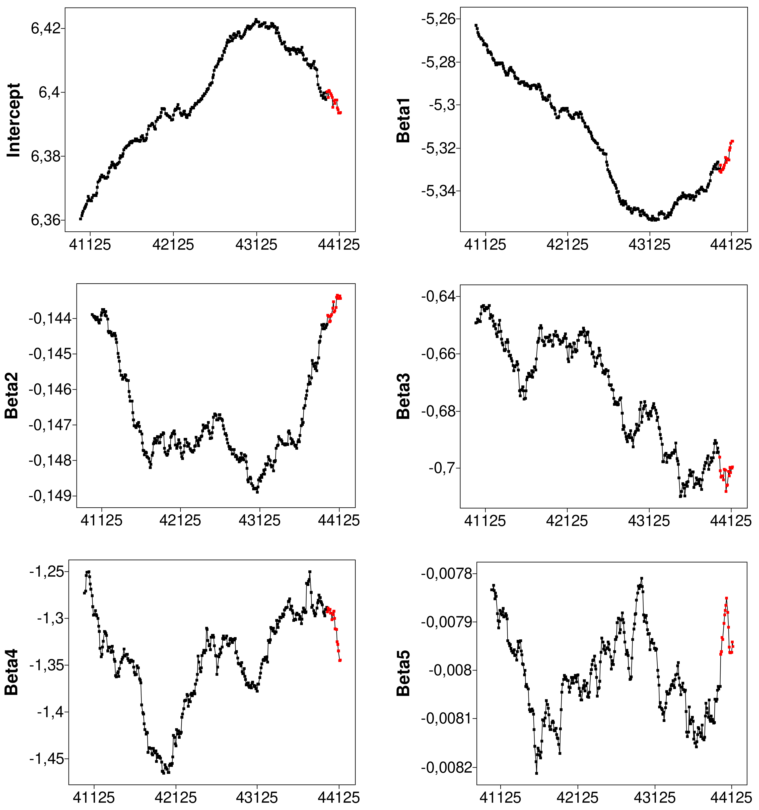
The results in the table for the batch analysis are complemented by the forward plots of the six parameter estimates in Figure 9, with the outlying observations plotted in red (in the online .pdf version). Since the batch search moves forward in batches of ten observations, the values are only plotted in steps of ten, when ${\widehat{\beta }}_j\left(m_b\right)$ is evaluated for each member of ${\mathcal{M}}_b$. The first three panels (those for the intercept, ${\beta }_1$ and ${\beta }_2$) reveal that the deleted observations were continuing trends in the parameter estimates that showed over the last 1000 observations. On the other hand, the other three panels, for statistically less significant variables, show that the outliers were altering the parameter estimates in a less systematic manner.

Figure 9, together with the results in Table 1, show that the SAS batch FS leads to similar inferential results to those of the implementation of the MATLAB FS in FSDA. Section 6 shows typical time savings from using our SAS program and further saving from working with batches. The major statistical difference is that, in this example, the batch FS marks a few more observations as outlying than the standard search does. This occurs because the batches of k values of the mdr are all calculated from the same parameter estimates, thus producing values more extreme than those when $k=1$ and the parameters are re-estimated for each deletion residual.

Our overall conclusion, from these and other data analyses, is that the SAS batch forward search allows faster analysis of large datasets and the analysis of larger datasets than other forward search algorithms. We have also demonstrated that the value $k=10$ has a negligible effect on the results of statistical analyses for sample sizes where the batch procedure yields a significant reduction in computational time.

8. Discussion and Extensions

The main emphasis in our paper is on the SAS version of the FS for regression and its extension to the batch FS for large datasets. We now consider other contributions of fsdaSAS for data analysis. We start with a comparison of methods of robust regression, before moving on to the monitoring methods we have made available and their application to a number of aspects of multivariate analysis and to model choice.

8.1. Three Classes of Estimator for Robust Regression

It is helpful to divide methods of robust regression into three classes.

• Hard (0,1) trimming: In least trimmed squares (LTS: [17,18]) the amount of trimming is determined by the choice of the trimming parameter h, $[n/2]+\left[\right(p+1)/2]\le h\le n$, which is specified in advance. The LTS estimate is intended to minimise the sum of squares of the residuals of h observations. For LS, $h=n$. We also monitor a generalisation of least median of squares (LMS, [18]) in which the estimate of the parameters minimises the median of h squared residuals.
• Adaptive hard trimming: In the FS, the observations are again hard trimmed, but the value of h is determined by the data, being found adaptively by the search. (See [19,20] for regression, [21] for a general survey of the FS, with discussion, and [22] for results on consistency).
• Soft trimming (downweighting): M estimation and derived methods. The intention is that observations near the centre of the distribution retain their value, but the $\rho$ function ensures that increasingly remote observations have a weight that decreases with distance from the centre. SAS provides the ROBUSTREG procedure where the choice of downweighting estimators includes S [23] and MM estimation [24] independently of the $\rho$ function (Andrews, Bisquare, Cauchy, Fair, Hampel, Huber, Logistic, Median, Talworth, Welsch). Our contribution is the monitoring of these estimators and also of LTS and LMS (as described in the section below).
  Many of the algorithms for finding these estimators start from very small subsets of data, typically of size p or $p+1$, before moving on to the use of larger subsets. Hawkins and Olive [25] argue that, to avoid inconsistent estimators, these larger subsets need to increase in size with n. Cerioli et al. [22] prove the consistency of the FS. In addition to developing the analysis of consistency, Olive [26] discusses the approximate nature of the estimators from subset procedures and analyses the computational complexity of the exact solutions to some of these robust estimation problems.

8.2. Monitoring and Graphics

The series of fits provided by the FS is combined with an automatic procedure for outlier detection that leads to the adaptive data-dependent choice of highly efficient robust estimates. It also allows monitoring of residuals and parameter estimates for fits of differing robustness. Linking plots of such quantities, combined with brushing, provides a set of powerful tools for understanding the properties of data including anomalous structures and data points. Our SAS package extends this idea of monitoring to several traditional robust estimators of regression for a range of values of their key parameters (maximum possible breakdown or nominal efficiency). We again obtain data-adaptive values for these parameters and provide a variety of plots linked through brushing. Examples in Torti et al. [3] are for S estimation and for least median of squares (LMS) and least trimmed squares (LTS) regression. These two forms of monitoring are currently only available in our SAS toolbox.

We monitor using either the theoretical breakdown point (bdp) or the efficiency of the estimators. For LTS and LMS, we vary the trimming proportion $\alpha$ from 0.5 to 0. Then, the theoretical bdp is $\alpha$, which is zero for no trimming. However, the efficiency decreases as $\alpha$ increases. It is not possible to have an estimator which simultaneously has maximum bdp and 100% efficiency. We now outline the results showing that a similar restriction applies to soft trimming estimators.

Rousseeuw and Leroy [27] (p. 139) give conditions to be obeyed by the symmetric function $\rho$. One is that there should be a $c>0$ such that $\rho$ is strictly increasing on $[0,c]$ and constant on $[c,\infty )$. We monitor S estimators by looking over a grid of values of bdp. The breakdown point of the S-estimator tends to bdp when $n\to \infty$. As c increases, fewer observations are downweighted, so that the estimates of the parameters approach those for least squares and bdp $\to 0$. Riani et al. [28] shows that the choice of the value of c determines both the bdp and efficiency of the estimator, although the exact values depend upon the specific $\rho$ function. The dependence of both bdp and efficiency on the value of c again means that, as for hard trimming, it is impossible to have an estimator with high values of both asymptotic properties. Riani et al. [28] (Section 3.1) give computationally efficient calculations for finding the value of c for Tukey’s bisquare once the value of bdp is specified. For MM estimators, we instead monitor efficiency. The calculations to find c for given efficiency are given in their Section 3.2. Riani et al. [29] shows plots exhibiting the relationship between bdp and efficiency for five $\rho$ functions. A much fuller discussion of monitoring robust regression is [4], including examples of S, MM, LMS and LTS analyses using the FSDA.

For estimators other than the FS, monitoring takes the form of inspecting, either visually or automatically using correlation measures, the monitoring plots of scaled residuals, such as that in Figure 2, to determine where the pattern of residuals changes. For multivariate data, ref [30] monitor the values of Mahalanobis distances. As a result adaptive values of trimming parameters or bdp can be found which, for a particular dataset, yield the most efficient robust parameter estimates. Since the standard distribution of SAS does not provide graphical interactivity for exploratory data analysis and satisfactory graphical output, we used a separate package based on the IML language (SAS/IML Studio) to realise in SAS a number of FSDA functions requiring advanced graphical output and interactivity.

8.3. Programs

The programs we provided in SAS/IML Studio are being protected under the European Union Public License and are therefore open source and GPL compatible. We have here had only space to exhibit a few of these programs, which are further discussed in Torti et al. [3]. They include:

• FSR.sx and FSM.sx, which implement the FS approach to detect outliers, respectively, in regression and in multivariate data;
• FSRfan.sx and FSMfan.sx for identifying the best transformation parameter for the Box–Cox transformation in regression and multivariate analysis ([31], Chapter 4);
• Monitoring.sx for monitoring a number of traditional robust multivariate and regression estimators (S, MM, LTS and LMS), already present in SAS, for specific choices of breakdown point or efficiency. Riani et al. [4] introduced the monitoring of regression estimators detailed in Section 8.2, however, in the FSDA toolbox, only for S and MM estimators (and the FS) in MATLAB. The extension to the monitoring of LTS and LMS is a particularly powerful new feature and a novelty in the statistical literature.

We also modified the standard LTS and LMS IML functions by introducing the small sample correction factor of Pison [32] and by increasing the range of values of the trimming parameter h in LTS.

Further developments which there is no space to describe here include:

• FSM.sx, the multivariate counterparts of FSR, and FSMfan.sx for multivariate transformations;
• FSRms.sx for choosing the best model in regression. This function implements the procedure of Riani and Atkinson [33] which combines Mallows’ $C_p$ [34] with the flexible trimming of the FS to yield an information rich plot “The Generalized Candlestick Plot” revealing the effect of outliers on model choice;
• FSRMultipleStart.sx and FSMmultiplestart.sx for identifying observations that are divided into groups either of regression models or of multivariate normal clusters. The later procedure is derived from the FSDA implementation of Atkinson et al. [35].

In addition to programming, our main methodological advance is the batch procedure described in Section 5 which provides a computationally fast version of the FS taking advantage of the ability of SAS to handle datasets much larger than those analysable by R or in the MATLAB FSDA tool box, with little loss in statistical efficiency. Appendix C contains comments on other software for robust statistical analysis.

References

1. Perrotta, D.; Riani, M.; Torti, F. New robust dynamic plots for regression mixture detection. Adv. Data Anal. Classif. 2009, 3, 263–279. [Google Scholar] [CrossRef]
2. Riani, M.; Perrotta, D.; Torti, F. FSDA: A MATLAB toolbox for robust analysis and interactive data exploration. Chemom. Intell. Lab. Syst. 2012, 116, 17–32. [Google Scholar] [CrossRef]
3. Torti, F.; Perrotta, D.; Atkinson, A.C.; Corbellini, A.; Riani, M. Monitoring Robust Regression in SAS IML Studio: S, MM, LTS, LMS and Especially the Forward Search; Technical Report JRC121650; Publications Office of the European Union: Luxembourg, 2020. [Google Scholar]
4. Riani, M.; Cerioli, A.; Atkinson, A.C.; Perrotta, D. Monitoring Robust Regression. Electron. J. Stat. 2014, 8, 642–673. [Google Scholar] [CrossRef]
5. Riani, M.; Atkinson, A.C.; Cerioli, A. Finding an Unknown Number of Multivariate Outliers. J. R. Stat. Soc. Ser. B 2009, 71, 447–466. [Google Scholar] [CrossRef] [Green Version]
6. Atkinson, A.C.; Riani, M.; Corbellini, A. An analysis of transformations for profit-and-loss data. Appl. Stat. 2020, 69, 251–275. [Google Scholar] [CrossRef]
7. Atkinson, A.C.; Riani, M. Distribution theory and simulations for tests of outliers in regression. J. Comput. Graph. Stat. 2006, 15, 460–476. [Google Scholar] [CrossRef]
8. Atkinson, A.C. Testing transformations to normality. J. R. Stat. Soc. Ser. B 1973, 35, 473–479. [Google Scholar] [CrossRef]
9. Riani, M.; Atkinson, A.C. Robust diagnostic data analysis: Transformations in regression (with discussion). Technometrics 2000, 42, 384–398. [Google Scholar] [CrossRef]
10. Atkinson, A.C.; Riani, M. Tests in the fan plot for robust, diagnostic transformations in regression. Chemom. Intell. Lab. Syst. 2002, 60, 87–100. [Google Scholar] [CrossRef] [Green Version]
11. Atkinson, A.C.; Corbellini, A.; Riani, M. Robust Bayesian Regression with the Forward Search: Theory and Data Analysis. Test 2017, 26, 869–886. [Google Scholar] [CrossRef] [Green Version]
12. Cerioli, A.; Riani, M. Robust methods for the analysis of spatially autocorrelated data. Stat. Methods Appl. J. Ital. Stat. Soc. 2002, 11, 335–358. [Google Scholar] [CrossRef]
13. Maitra, R.; Melnykov, V. Simulating Data to Study Performance of Finite Mixture Modeling and Clustering Algorithms. J. Comput. Graph. Stat. 2010, 19, 354–376. [Google Scholar] [CrossRef] [Green Version]
14. Torti, F.; Perrotta, D.; Riani, M.; Cerioli, A. Assessing Trimming Methodologies for Clustering Linear Regression Data. Adv. Data Anal. Classif. 2018. [Google Scholar] [CrossRef] [Green Version]
15. Corbellini, A.; Magnani, M.; Morelli, G. Labor market analysis through transformations and robust multivariate models. Socio-Econ. Plan. Sci. 2020. [Google Scholar] [CrossRef]
16. Breiman, L.; Friedman, J.H. Estimating optimal transformations for multiple regression and transformation (with discussion). J. Am. Stat. Assoc. 1985, 80, 580–619. [Google Scholar] [CrossRef]
17. Hampel, F.R. Beyond location parameters: Robust concepts and methods. Bull. Int. Stat. Inst. 1975, 46, 375–382. [Google Scholar]
18. Rousseeuw, P.J. Least median of squares regression. J. Am. Stat. Assoc. 1984, 79, 871–880. [Google Scholar] [CrossRef]
19. Atkinson, A.C.; Riani, M. Robust Diagnostic Regression Analysis; Springer: New York, NY, USA, 2000. [Google Scholar]
20. Riani, M.; Atkinson, A.C.; Perrotta, D. A parametric framework for the comparison of methods of very robust regression. Stat. Sci. 2014, 29, 128–143. [Google Scholar] [CrossRef]
21. Atkinson, A.C.; Riani, M.; Cerioli, A. The Forward Search: Theory and data analysis (with discussion). J. Korean Stat. Soc. 2010, 39, 117–134. [Google Scholar] [CrossRef]
22. Cerioli, A.; Farcomeni, A.; Riani, M. Strong consistency and robustness of the Forward Search estimator of multivariate location and scatter. J. Multivar. Anal. 2014, 126, 167–183. [Google Scholar] [CrossRef]
23. Rousseeuw, P.J.; Yohai, V.J. Robust regression by means of S-estimators. In Robust and Nonlinear Time Series Analysis: Lecture Notes in Statistics 26; Springer: New York, NY, USA, 1984; pp. 256–272. [Google Scholar]
24. Yohai, V.J.; Zamar, R.H. High breakdown-point estimates of regression by means of the minimization of an efficient scale. J. Am. Stat. Assoc. 1988, 83, 406–413. [Google Scholar] [CrossRef]
25. Hawkins, D.M.; Olive, D.J. Inconsistency of resampling algorithms for high-breakdown regression estimators and a new algorithm (with discussion). J. Am. Stat. Assoc. 2002, 97, 136–159. [Google Scholar] [CrossRef] [Green Version]
26. Olive, D.J. Robust Statistics. 2020. Available online: http://parker.ad.siu.edu/Olive/robbook.htm (accessed on 15 April 2021).
27. Rousseeuw, P.J.; Leroy, A.M. Robust Regression and Outlier Detection; Wiley: New York, NY, USA, 1987. [Google Scholar]
28. Riani, M.; Cerioli, A.; Torti, F. On consistency factors and efficiency of robust S-estimators. Test 2014, 23, 356–387. [Google Scholar] [CrossRef]
29. Riani, M.; Atkinson, A.C.; Corbellini, A.; Perrotta, D. Robust regression with density power divergence: Theory, comparisons and data analysis. Entropy 2020, 22, 399. [Google Scholar] [CrossRef] [Green Version]
30. Cerioli, A.; Riani, M.; Atkinson, A.C.; Corbellini, A. The power of monitoring: How to make the most of a contaminated multivariate sample (with discussion). Stat. Methods Appl. 2017. [Google Scholar] [CrossRef]
31. Atkinson, A.C.; Riani, M.; Cerioli, A. Exploring Multivariate Data with the Forward Search; Springer: New York, NY, USA, 2004. [Google Scholar]
32. Pison, G.; Van Aelst, S.; Willems, G. Small sample corrections for LTS and MCD. Metrika 2002, 55, 111–123. [Google Scholar] [CrossRef] [Green Version]
33. Riani, M.; Atkinson, A.C. Robust model selection with flexible trimming. Comput. Stat. Data Anal. 2010, 54, 3300–3312. [Google Scholar] [CrossRef] [Green Version]
34. Mallows, C.L. Some comments on Cp. Technometrics 1973, 15, 661–675. [Google Scholar]
35. Atkinson, A.C.; Riani, M.; Cerioli, A. Cluster detection and clustering with random start forward searches. J. Appl. Stat. 2018, 45, 777–798. [Google Scholar] [CrossRef]
36. Lehmann, E. Point Estimation; Wiley: New York, NY, USA, 1991. [Google Scholar]
37. Guenther, W.C. An Easy Method for Obtaining Percentage Points of Order Statistics. Technometrics 1977, 19, 319–321. [Google Scholar] [CrossRef]
38. Johnson, N.L.; Kotz, S.; Balakrishnan, N. Continuous Univariate Distributions—1, 2nd ed.; Wiley: New York, NY, USA, 1994. [Google Scholar]
39. Tallis, G.M. Elliptical and Radial Truncation in Normal Samples. Ann. Math. Stat. 1963, 34, 940–944. [Google Scholar] [CrossRef]
40. Buja, A.; Rolke, W. Calibration for Simultaneity: (Re)Sampling Methods for Simultaneous Inference with Applications to Function Estimation and Functional Data; Technical Report; The Wharton School, University of Pennsylvania: Philadelphia, PA, USA, 2003. [Google Scholar]
41. Todorov, V.; Filzmoser, P. An Object-Oriented Framework for Robust Multivariate Analysis. J. Stat. Softw. 2009, 32, 1–47. [Google Scholar] [CrossRef] [Green Version]
42. Rousseeuw, P.J.; Croux, C.; Todorov, V.; Ruckstuhl, A.; Salibian-Barrera, M.; Verbeke, T.; Maechler, M. Robustbase: Basic Robust Statistics. R Package Version 0.92-7. 2009. Available online: http://CRAN.R-project.org/package=robustbase (accessed on 15 April 2021).
43. Riani, M.; Cerioli, A.; Corbellini, A.; Perrotta, D.; Torti, F.; Sordini, E.; Todorov, V. fsdaR: Robust Data Analysis Through Monitoring and Dynamic Visualization. 2017. Available online: https://CRAN.R-project.org/package=fsdaR (accessed on 15 April 2021).
44. Hubert, M.; Debruyne, M. Minimum Covariance Determinant. Wires Comput. Stat. 2010, 2, 36–43. [Google Scholar] [CrossRef]
45. Vanden Branden, K.; Hubert, M. Robustness properties of a robust partial least squares regression method. Anal. Chim. Acta 2005, 515, 229–241. [Google Scholar] [CrossRef]
46. Verboven, S.; Hubert, M. Matlab library LIBRA. Wires Comput. Stat. 2010, 2, 509–515. [Google Scholar] [CrossRef]
47. Hubert, M.; Rousseeuw, P.J.; Vanden Branden, K. ROBPCA: A new approach to robust principal component analysis. Technometrics 2005, 47, 64–79. [Google Scholar] [CrossRef]
48. García-Escudero, L.A.; Gordaliza, A.; Matran, C.; Mayo-Iscar, A.; San Martin, R. A general trimming approach to robust cluster analysis. Ann. Stat. 2008, 36, 1324–1345. [Google Scholar] [CrossRef]
49. García-Escudero, L.A.; Gordaliza, A.; Mayo-Iscar, A.; San Martin, R. Robust clusterwise linear regression through trimming. Comput. Stat. Data Anal. 2010, 54, 3057–3069. [Google Scholar] [CrossRef]
50. Maronna, R.A.; Martin, R.D.; Yohai, V.J. Robust Statistics: Theory and Methods; Wiley: Chichester, UK, 2006. [Google Scholar]
51. Van Aelst, S.; Rousseeuw, P.J. Minimum volume ellipsoid. Wires Comput. Stat. 2009, 1, 71–82. [Google Scholar] [CrossRef]
Figure 1. Example of the SAS IML Studio code which uploads the loyalty card data in SAS IML.
Stats 04 00022 g001
Figure 2. Loyalty card data: monitoring plots for the transformed data with λ = 0.4 . The top panel shows the absolute values of minimum deletion residuals among observations not in the subset; the last part of the curve, corresponding to the 18 identified outliers, is automatically highlighted in red (in the online .pdf version). The bottom panel shows the scaled residuals, with the trajectories corresponding to the 18 detected outliers automatically represented in red (in the online .pdf version). The box under each panel contains the SAS code used to generate the plot.
Stats 04 00022 g002
Figure 3. Loyalty card data with λ = 0.4 : zoom of Figure 2 monitoring the last 30 observations. Absolute values of minimum deletion residuals among observations not in the subset and envelopes for the full 509 observations. Lower panel: scaled residuals, with the trajectories corresponding to the 18 detected outliers in red.
Stats 04 00022 g003
Figure 4. Loyalty card data: scatterplots of transformed data when λ = 0.4 , with the 18 outliers detected plotted as red crosses (in the online .pdf version). Last panel: a plot, suggested by a referee, of the fitted values on the horizontal axis and the response on the vertical axis. The box under the figure contains the SAS code used to generate the scatterplots.
Stats 04 00022 g004
Figure 5. Loyalty card data: monitoring of the estimated beta coefficients on transformed data when λ = 0.4 , with the part of the trajectory corresponding to the 18 detected outliers highlighted in red (in the online .pdf version). The box under the figure contains the SAS code used to generate the plots.
Stats 04 00022 g005
Figure 6. Two artificial datasets generated with MixSim for the assessment: 4750 observations from the dominant linear component (blue dots) + 250 observations from a contaminating linear component (black stars) + 150 observations from uniform contamination (red crosses).
Stats 04 00022 g006
Figure 7. Top panel: boxplots showing, for different values of k (the fs_step parameter, on the x axis), the bias and dispersion of the estimated slopes and intercepts (respectively from left to right for each k). The estimates are obtained from 500 simulated datasets of 5150 observations; Bottom panel: percentage of estimated values lying outside the boxplot whiskers for slope (blue asterisks) and intercept (black circles).
Stats 04 00022 g007
Figure 8. Execution time of our SAS (Version R9.4) and MATLAB (R2020a) implementations of the FSR function; for SAS, the comparison is also with the batch version of FSR (with k = 10 ). The assessment covers data with one explanatory variable and size ranging from 30 to 100,000. Results are split into three panels for small, medium and large data sizes. The last, bottom-right, panel gives the ratio between the time required by the MATLAB implementation and the two SAS ones. The associated table reports the time in seconds for selected sample sizes.
Stats 04 00022 g008
Figure 9. SAS batch analysis of balance sheet data: monitoring of estimated beta coefficients on transformed data, starting from 41 , 000 units with the part of the trajectory corresponding to the 161 detected outliers, highlighted in red (in the online .pdf version).
Stats 04 00022 g009