Article

Structural Stability Analysis of Proteins Using End-to-End Distance: A 3D-RISM Approach

by
Yutaka Maruyama
1,2,† and
Ayori Mitsutake
2,*,†
1
Quemix Inc., 2-11-2 Nihombashi, Chuo-ku, Tokyo 103-0027, Japan
2
Department of Physics, School of Science and Technology, Meiji University, 1-1-1 Higashi-Mita, Tama-ku, Kawasaki-shi 214-8571, Japan
*
Author to whom correspondence should be addressed.
These authors contributed equally to this work.
J 2022, 5(1), 114-125; https://doi.org/10.3390/j5010009
Submission received: 28 January 2022 / Revised: 6 February 2022 / Accepted: 7 February 2022 / Published: 14 February 2022
(This article belongs to the Special Issue Advance in Molecular Thermodynamics)

Abstract

:
The stability of a protein is determined from its properties and surrounding solvent. In our previous study, the total energy as a sum of the conformational and solvation free energies was demonstrated to be an appropriate energy function for evaluating the stability of a protein in a protein folding system. We plotted the various energies against the root mean square deviation, required as a reference structure. Herein, we replotted the various energies against the end-to-end distance between the N- and C-termini, which is not a required reference and is experimentally measurable. The solvation free energies for all proteins tend to be low as the end-to-end distance increases, whereas the conformational energies tend to be low as the end-to-end distance decreases. The end-to-end distance is one of interesting measures to study the behavior of proteins.

1. Introduction

AlphaFold2 [1] and RoseTTAFold [2], which are protein structure software programs using amino acid sequences, have shown a high level of accuracy. In addition, DeepMind and EMBL’s European Bioinformatics Institute have created a database of 21 model-organism proteome structures for free use by the academic community [3]. The development and movement of protein structure prediction have increased the importance of protein-structure-based methods. For example, it is necessary to select reasonable and stable structures from among predicted structure candidates by incorporating the solvent effect. Moreover, it is difficult to investigate structural fluctuations and conformational changes in a protein, which can affect their functions, using prediction software. It is important to investigate the structural stability, including the solvent effect during conformational changes and the protein-folding process. The three-dimensional reference interaction site model (3D-RISM), which is the statistical mechanical theory for molecular liquids, is one of the structure-based methods applied [4,5]. The 3D-RISM theory provides the distribution functions of a solvent around a biomolecule such as a protein using the solute molecule structure as input. We can know the position of water [6,7,8] or ions [9,10,11] around the protein from the distribution function. In this way, we can calculate the physical quantity of the surrounding solvent around the protein, and in particular, estimate the stability of the proteins.
In a previous study [12], we discussed the structural stability of proteins performed on Anton’s molecular dynamics (MD) simulation trajectory [13]. For many structural calculations, we summarized that the sum of the conformational energy and solvation free energy using 3D-RISM theory is a reasonable indicator of protein structural stability. In the previous study, we plotted various energies as a function of the root-mean-square deviation (RMSD) for atomic C α positions. This is a useful approach for investigating the structural stability of a protein [14,15,16,17,18]. However, the reference structure of RMSD, which, in this case, is a native structure, must be known in advance. We also plotted various energies against the radius of gyration in the Supporting Information in Ref. [12]. The radius of gyration is a physical quantity that can be measured experimentally and calculated without the reference structure. Plots against the radius of gyration are used to study the protein stability as well as the RMSD [19,20,21,22]. Figure 1 shows the C α -RMSD against the radius of gyration for the four proteins (see also Ref. [12]). It can be seen that the vertical distribution of all proteins is concentrated at a certain value of the radius of gyration. The value of the radius of gyration settles to approximately the same value when the protein becomes compact. It might be difficult to compare the stabilities between native and compact structures, whereas the radius of gyration is one of appropriate physical quantities for investigating stabilities.
A fluorescent resonance energy transfer (FRET) is a useful technique for studying the conformational distribution and dynamics of biological molecules. FRET, detected at the single-molecule level, provides new opportunities to investigate the detailed kinetics of structural changes [23,24,25]. A sequential data assimilation method for single-molecule FRET data combined with MD simulations was developed by Matsunaga et al. [26], who also devised a machine learning method to combine the complementary information from single-molecule FRET experiments and an MD simulation to construct a consistent model of conformational dynamics [27,28,29]. It has become possible to associate information on the distance between fluorescent molecules obtained from FRET with structural information at the atomic level through an MD simulation. Thus, we can observe information regarding the end-to-end distance between the N- and C-termini of a protein through experiments such as FRET.
In the present study, we attempted to analyze the various energies of proteins as a function of the end-to-end distance, which does not require the reference structure and is experimentally measurable. From the analysis, the solvation free energy as a function of the end-to-end distance has a characteristic tendency among four proteins.

2. Computational Details
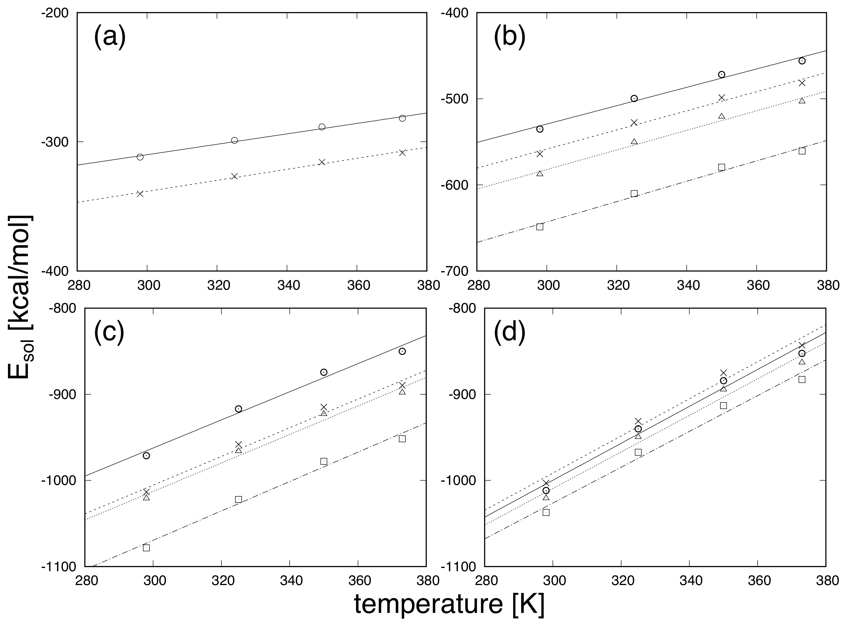
As in our previous study, we used the following four proteins: superchignolin (a small protein, CLN025), the WW domain variant GTT (a β -sheet protein, mGTT), a triple mutant of the redesigned protein G variant NuG2 (an α + β protein, mNuG2), and the de novo-designed three-helix bundle protein α 3D (an α -helical protein, m α 3D). The details of Anton’s MD simulations for these proteins can be found in the Supporting Information in [13]. In addition, CLN025, mGTT, mNuG2, and m α 3D contain 10, 35, 56, and 73 amino acids, respectively.
To investigate the structural stability of the proteins, we introduce the total energy E tot , which is the sum of the conformational energy E conf , and the solvation free energy (SFE) E sol :
E tot = E conf + E sol .
We used GROMACS [30] for calculating the conformational energy with a CHARMM22* force field [31,32,33]. The SFE of the proteins is calculated using the 3D-RISM theory based on the reference-modified density functional theory [34]. The number densities of water and the optimal hard sphere diameters used for the thermodynamic states at 298, 325, 350, and 373 K are shown in Table 1 (See Ref. [35]). We conducted an SFE calculation using the 3D-RISM theory with the original code written for a GPU [36]. An SFE calculation of a mNuG2 protein takes within 10 s on NVIDIA V100 GPU (256 3 grids, water solvent).
The structures were applied every 20 ns (every 100 samples) for CLN025 and every 200 ns (every 1000 samples) for the others when extracted from Anton’s trajectory during the calculations. The total numbers of sampling structures are 5348, 5686, 5780, and 3534 for CLN025, mGTT, mNuG2, and m α 3D, respectively. For the C α -RMSD calculations, the reference structures were taken from the Supporting Information provided by Honda et al. [37], i.e., 2F21.pdb, 1MIO.pdb, and 2A3D.pdb for CLN025, mGTT, mNuG2, and m α 3D, respectively. These structures correspond to the native structures. The end-to-end distance is defined as the distance between the C α atoms of the N- and C-termini.
Table 1. Experimental number density of water [38] and optimal diameters of the hard sphere diameter for SFE calculations with the reference-modified density functional theory at several temperatures along 1 atm [35].
Temperature [K]Number Density [Å 3 ]Diameter [Å]
2980.0333292.87500
3250.0329942.87125
3500.0325262.87000
3750.0319242.87250

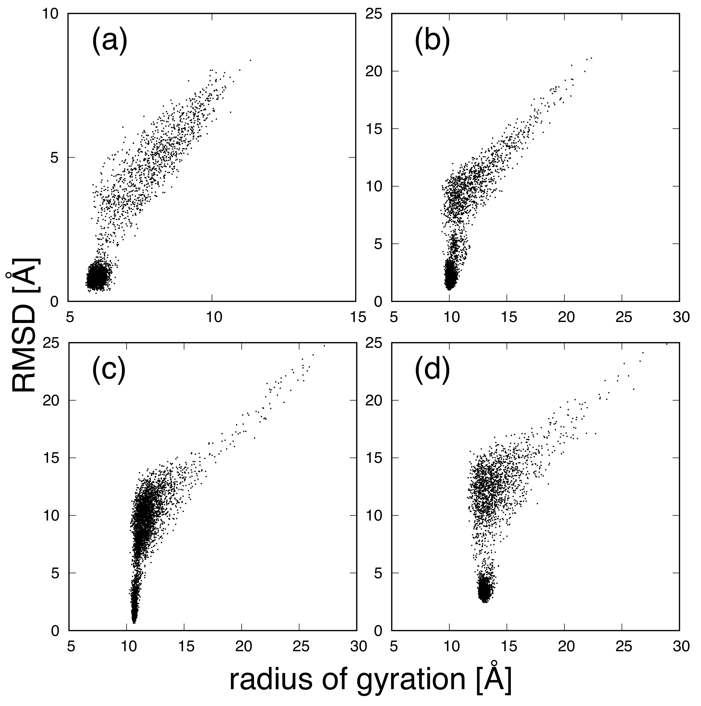
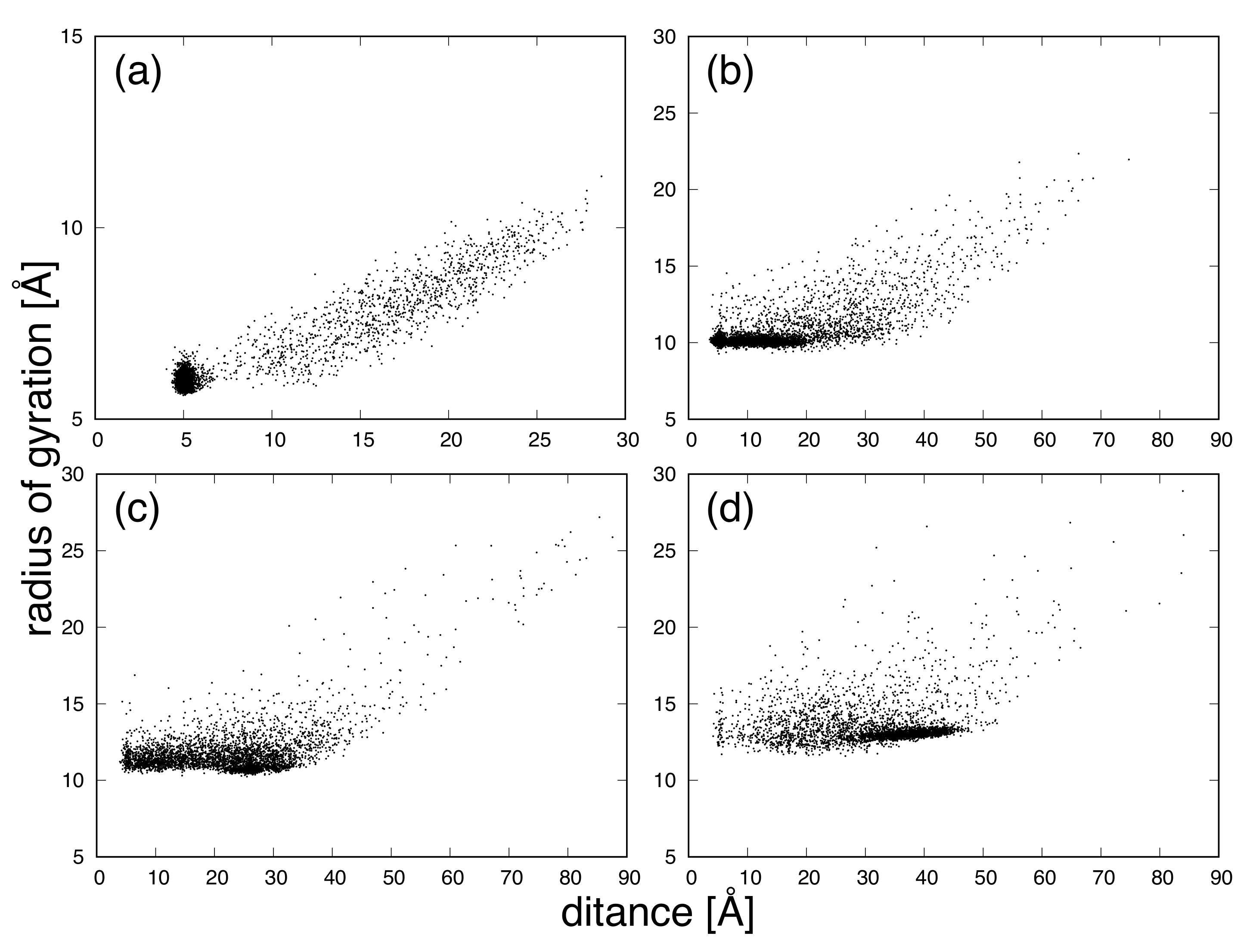
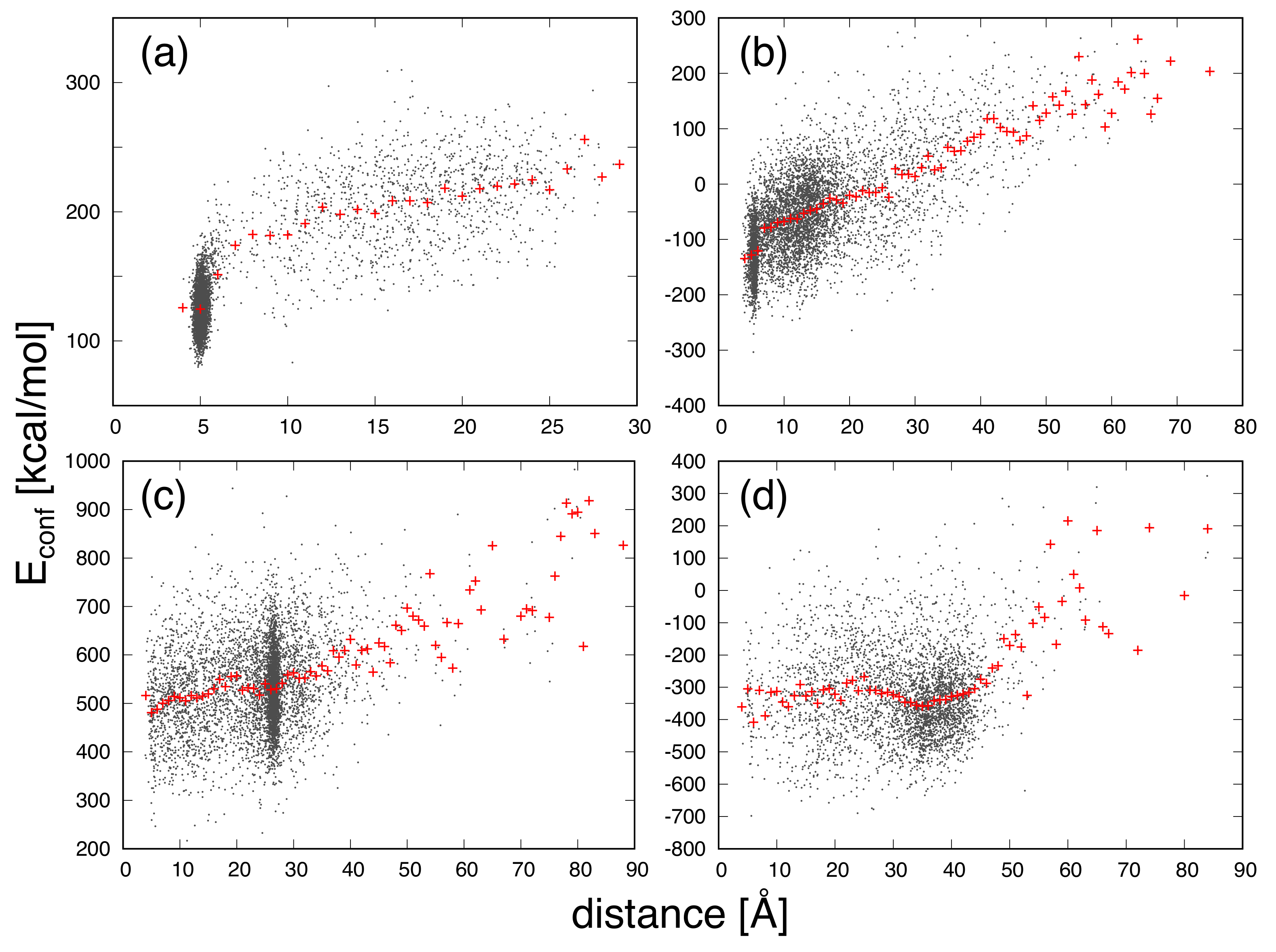
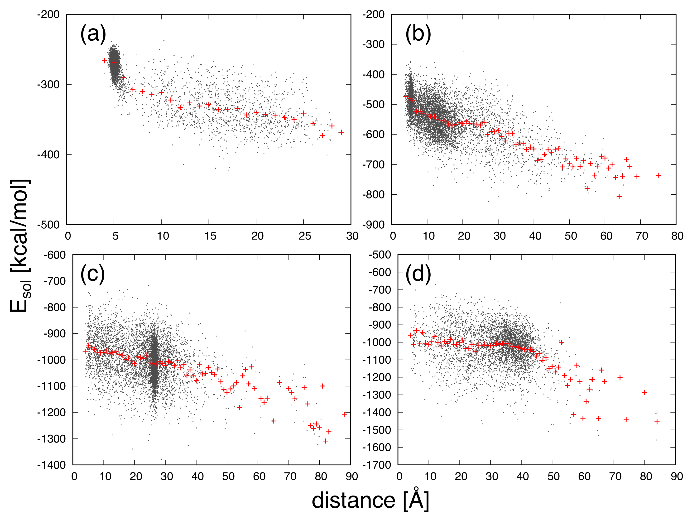
3. Results and Discussion

First, we show the lowest-total-energy and shortest end-to-end distance structures of the four proteins in Figure 2. In Table 2, C α -RMSD, the radius of gyration, the end-to-end distance, and the total energy of the two structures for each protein are listed. For the four proteins, the lowest-total-energy structures correspond to the native structures. The lowest-total energy and the shortest end-to-end distance structures are compact because the values of the radius of gyration for two structures are small and similar to each other for four proteins as listed in Table 2.
For CLN025 (Figure 2a,b) and mGTT (Figure 2c,d), the shortest end-to-end distance structures are similar to the native structures because C α -RMSD for the shortest end-to-end distance is small and similar to that for the lowest-total-energy distance. The native structures tend to have short end-to-end distances. Note that even though the lowest total energy and shortest end-to-end distance structures are similar, the total energy values are different, as listed in Table 2.
By contrast, for mNuG2 ((e,f)) and m α 3D ((g,h)), there is a large difference between the native and shortest end-to-end distance structures, as shown in Figure 2. The C α -RMSDs for the shortest end-to-end distances were large. The lowest-total-energy structures of these proteins tend to have slightly larger end-to-end distances. Because of the different structures, a large difference in the total energy between the lowest total energy and shortest end-to-end distance structures was also observed.
We examine the relationships between the radius of gyration and end-to-end distance and between C α -RMSD and end-to-end distance in the four proteins in Figure 3 and Figure 4, respectively. For CLN025, the radius of gyration and end-to-end distance appeared to have a positive correlation as shown in Figure 3. The reason is the simple structure, which is a turn one for CLN025. For mGTT, mNuG2, and m α 3D, the structures with small values of the radius of gyration were spread in the end-to-end distance direction. In the folding trajectories, many compact structures were generated. For the proteins with complicated structures, the end-to-end distance distinguishes the compact structures.
In Figure 4, the distributions for the end-to-end distance are different for all proteins, whereas those for the radius of gyration are similar to each other, as shown in Figure 1. Because the native structures are energetically stable and occur frequently during simulations, the point-concentrated areas correspond to the native structures, which have low RMSDs. For CLN025, shown in Figure 4a, the point-concentrated area corresponds to the shortest end-to-end distance and the lowest C α -RMSD. The C α -RMSD and end-to-end distance appeared to have a positive correlation. However, for mGTT, shown in Figure 4b, the lowest C α -RMSD structures were spread in the end-to-end distance direction from 5 to 20 Å. This indicates that the structures in the area are close to stable, but the N- or C-termini fluctuate. For mNuG2, shown in Figure 4c, the point-concentrated area was narrow and corresponded to a slightly large end-to-end distance (approximately 27 Å). For m α 3D, shown in Figure 4d, the point-concentrated area is spread along the end-to-end distance from 30 to 45 Å. As shown above, the behaviors of the end-to-end distance within the vicinity of the most stable structure are different for the four proteins. The relationship between C α -RMSD and end-to-end distance depends on the protein. For mGTT, mNuG2, and m α 3D, structures with a similar end-to-end distance include not only the native structure but also other structures. It is difficult to use the end-to-end distance for identifying the native structure without the reference. However, the conformational energy and the solvation free energy as functions of the end-to-end distance have characteristics as explained below.
Figure 5 shows the total energy of each protein as a function of the end-to-end distance. The patterns of the point distribution for the end-to-end distance were different for the four proteins, whereas those for the C α -RMSD are similar, as shown in Figure 2 of Ref. [12]. The ranges of the total energy of CLN025, mGTT, mNuG2, and m α 3D, shown in Figure 5a–d, respectively, are approximately 100, 180, 250, and 350 kcal/mol. The range of total energy expands as the protein size increases. The end-to-end distances for the point-concentrated areas corresponding to the native structures are 5 Å, 5 Å, 27 Å, and 30–45 Å for CLN025, mGTT, mNuG2, and m α 3D in Figure 5a–d, respectively. The broad distribution along the total energy within the regions are observed. For mGTT, shown in Figure 5d, the structures where the end-to-end distance is between 7 Å and 20 Åcorrespond to the native-like structure in which the N- or C-termini fluctuate. A broad distribution along the total energy of the regions was also observed.
The red point represents the average value of the total energy for each end-to-end distance. The average values for the regions of the native structures were lower than those of the other regions. The regions correspond to where the end-to-end distances are 5 Å, 5–20 Å, 27 Å, and 30–45 Å for CLN025, mGTT, mNuG2, and m α 3D, respectively. There were no significant changes in the average total energy within the region of the native structure. For CLN025 and mGTT, shown in Figure 5a,b, respectively, the average value increases as the end-to-end distance increases because the shortest end-to-end distance structures correspond to the lowest-energy structures. In addition, NuG2 and m α 3D, shown in Figure 5c,d, respectively, have different tendencies because the shortest end-to-end distance structures do not correspond to the lowest-energy structures.
Figure 6 shows the conformational energy of each protein as a function of the end-to-end distance. Conformational energy ranges of CLN025, mGTT, mNuG2, and m α 3D, shown in Figure 6a–d, respectively, were approximately 250, 600, 750, and 1100 kcal/mol. Compared to the total energy, the range of the conformational energy is wider because it competes with the SFE. The conformational energy and the SFE are inversely correlated, as shown in Figure 4d in Ref. [12]. The point-concentrated areas are similar to those for the total energy. The red point represents the average value of the conformational energy for each end-to-end distance.
For CLN025 and mGTT, shown in Figure 6a,b, respectively, the broad energy distributions near the stable states, where the end-to-end distances are 4–6 Å are also observed and are lower than those where the end-to-end distance is more than 7 Å. The average values rapidly decreased as the end-to-end distances decreased from 7 Å to 5 Å. The native structures with an end-to-end distance of 4–6 Å for both proteins had the lowest conformational energy. These results indicate that the conformational energy determines the stable structure of CLN025 and mGTT. For these proteins, the longer the end-to-end distance is, the higher the average conformational energy.
In Figure 6c,d, the broad energy distributions corresponding to the stable structures where the end-to-end distances are 24–25 Å for mNuG2 and 32–42 Å for m α 3D shift to higher positions, unlike those for the total energy. Similarly, the average values near the native structure are higher. The lowest conformational energy structures correspond to the shortest end-to-end structures. This means that the most stable structure is not determined by the conformational energy in mNuG2 and m α 3D. In particular, for m α 3D, there is no significant difference between the average values of the conformational energy when the end-to-end distance is less than 50 Å. For proteins, the longer the end-to-end distance is, the higher the average conformational energy. The conformational energy and end-to-end distance have a slight positive correlation.
Next, we show the SFE as a function of the end-to-end distance in Figure 7. The distribution of the SFE is close to an upside-down reversal of that of the conformational energy owing to mutual competition. However, a perfect upside-down symmetry is not shown because the SFE reflects hydrogen bond formations at the surface of the protein, whereas the conformational energy reflects the complex hydrogen bond formation within the protein. The SFE decreases as the end-to-end distance increases, not only for CLN025 and mGTT, as shown in Figure 7a,b, respectively, where the end-to-end distances of the stable states are small, but also for mNuG2 and m α 3D, shown in Figure 7c,d, where the end-to-end distances of the stable structures are large. Although the native structures of the four proteins have different end-to-end distances, the SFE as a function of the end-to-end distances has a similar tendency.
Finally, we show the temperature dependence of the average value of the SFE with different end-to-end distances in Figure 8. The triangles, crosses, and squares correspond to the average values of the SFE for end-to-end distances of 10, 20, 30, and 40 Å, respectively. Note that the conformational energy of a protein does not depend on temperature because the structures are extracted in the same simulations. The actual distribution of protein structures will be different when MD simulations are conducted at different temperatures. We ignored this point herein.
For a liquid phase of water at 1 atm, the SFE for structures with the same end-to-end distance is lower as the temperature is further decreased, as shown in Figure 8. The values of the slope for CLN025, mGTT, mNuG2, and m α 3D, shown in Figure 8, are approximately 0.4, 1.1, 1.7, and 2.1, respectively. Because the slope values for different end-to-end distance structures are similar, they do not depend on the end-to-end distances. The slope values depend on the protein size and increase as the protein becomes larger. The slope value at 10 Å is lower than that at 20 Å in m α 3D, shown in Figure 8d, because there are fewer sample points at below 10 Å, and the error at this value is large.

4. Conclusions

We investigated the energetics of proteins by plotting various energies against the end-to-end distance between the N- and C-termini, which does not require the reference structure and is experimentally measurable. We discussed how the end-to-end distance information of proteins can be incorporated into the stability of the proteins. The distributions of the total energy as a function of the end-to-end distance are different for the four proteins because native structures do not correspond to the shortest end-to-end distances. However, based on a number of calculations for all proteins, the characteristic behaviors of the distributions of the conformational energy and SFE were observed as the end-to-end distance increased. The solvation free energy tends to be low as the end-to-end distance increases, and the conformational energy tends to be high as the end-to-end distances decrease. The end-to-end distance is one of interesting measures for studying the behavior of proteins.
Here, we discuss the physical aspects of proteins as biopolymers. Proteins can be regarded as water-rich macromolecules. It is considered that the softness of polymers, in general, can be explained through entropic elasticity [40,41,42]. Polymer gels containing a large amount of water solvent are significantly softer than rubber without water and show a negative energy elasticity [43,44,45]. The microscopic origin of negative energy elasticity is the solvent–polymer interaction with the deformation of a polymer. When the polymer chain is mechanically stretched, the number of water molecules interacting with the chain increases, decreasing the total energy of the solvent–polymer interaction. The result in which the SFE decreases with an increase in the end-to-end distance might be related to the origin of the negative elastic energy of a polymer gel.

Author Contributions

Conceptualization, Y.M. and A.M.; methodology, Y.M.; software, Y.M.; validation, Y.M. and A.M.; formal analysis, Y.M.; writing—original draft preparation, Y.M.; writing—review and editing, Y.M. and A.M.; funding acquisition, A.M. All authors have read and agreed to the published version of the manuscript.

Funding

This work was supported by JSPS KAKENHI Grant Number JP20H03230.

Institutional Review Board Statement

Not applicable.

Informed Consent Statement

Not applicable.

Data Availability Statement

Not applicable.

Acknowledgments

Yutaka Maruyama would like to thank Sakumichi (The University of Tokyo, Japan) for the discussion on the negative energy elasticity of polymer gels. Numerical calculations were conducted in part using Cygnus at the Center for Computational Sciences, University of Tsukuba. Molecular graphics were designed using UCSF Chimera, which was developed by the Resource for Biocomputing, Visualization, and Informatics at the University of California, San Francisco.

Conflicts of Interest

The authors declare no conflict of interest.

Abbreviations

3D-RISMThree-dimensional reference interaction site model
MDMolecular dynamics
RMSDRoot-mean-square deviation
FRETFluorescent resonance energy transfer

References

  1. Jumper, J.; Evans, R.; Pritzel, A.; Green, T.; Figurnov, M.; Ronneberger, O.; Tunyasuvunakool, K.; Bates, R.; Žídek, A.; Potapenko, A.; et al. Highly accurate protein structure prediction with AlphaFold. Nature 2021, 596, 583–589. [Google Scholar] [CrossRef] [PubMed]
  2. Baek, M.; DiMaio, F.; Anishchenko, I.; Dauparas, J.; Ovchinnikov, S.; Lee, G.R.; Wang, J.; Cong, Q.; Kinch, L.N.; Schaeffer, R.D.; et al. Accurate prediction of protein structures and interactions using a three-track neural network. Science 2021, 373, 871–876. [Google Scholar] [CrossRef] [PubMed]
  3. Varadi, M.; Anyango, S.; Deshpande, M.; Nair, S.; Natassia, C.; Yordanova, G.; Yuan, D.; Stroe, O.; Wood, G.; Laydon, A.; et al. AlphaFold Protein Structure Database: Massively expanding the structural coverage of protein-sequence space with high-accuracy models. Nucleic Acids Res. 2021, 50, D439–D444. [Google Scholar] [CrossRef] [PubMed]
  4. Beglov, D.; Roux, B. An integral equation to describe the solvation of polar molecules in liquid water. J. Phys. Chem. B 1997, 101, 7821–7826. [Google Scholar] [CrossRef]
  5. Kovalenko, A.; Hirata, F. Three-dimensional density profiles of water in contact with a solute of arbitrary shape: A RISM approach. Chem. Phys. Lett. 1998, 290, 237–244. [Google Scholar] [CrossRef]
  6. Imai, T.; Hiraoka, R.; Kovalenko, A.; Hirata, F. Water molecules in a protein cavity detected by a statistical-mechanical theory. J. Am. Chem. Soc. 2005, 127, 15334–15335. [Google Scholar] [CrossRef]
  7. Sindhikara, D.J.; Yoshida, N.; Hirata, F. Placevent: An algorithm for prediction of explicit solvent atom distribution-Application to HIV-1 protease and F-ATP synthase. J. Comput. Chem. 2012, 33, 1536–1543. [Google Scholar] [CrossRef]
  8. Fusani, L.; Wall, I.; Palmer, D.; Cortes, A. Optimal water networks in protein cavities with GAsol and 3D-RISM. Bioinformatics 2018, 34, 1947–1948. [Google Scholar] [CrossRef]
  9. Yoshida, N.; Phongphanphanee, S.; Maruyama, Y.; Imai, T.; Hirata, F. Selective ion-binding by protein probed with the 3D-RISM theory. J. Am. Chem. Soc. 2006, 128, 12042–12043. [Google Scholar] [CrossRef]
  10. Yoshida, N.; Phongphanphanee, S.; Hirata, F. Selective ion binding by protein probed with the statistical mechanical integral equation theory. J. Phys. Chem. B 2007, 111, 4588–4595. [Google Scholar] [CrossRef]
  11. Maruyama, Y.; Matsushita, T.; Ueoka, R.; Hirata, F. Solvent and Salt Effects on Structural Stability of Human Telomere. J. Phys. Chem. B 2011, 115, 2408–2416. [Google Scholar] [CrossRef]
  12. Maruyama, Y.; Mitsutake, A. Stability of Unfolded and Folded Protein Structures Using a 3D-RISM with the RMDFT. J. Phys. Chem. B 2017, 121, 9881–9885. [Google Scholar] [CrossRef]
  13. Lindorff-Larsen, K.; Piana, S.; Dror, R.O.; Shaw, D.E. How fast-folding proteins fold. Science 2011, 334, 517–520. [Google Scholar] [CrossRef]
  14. Harano, Y.; Roth, R.; Sugita, Y.; Ikeguchi, M.; Kinoshita, M. Physical basis for characterizing native structures of proteins. Chem. Phys. Lett. 2007, 437, 112–116. [Google Scholar] [CrossRef]
  15. Kinoshita, M. Importance of translational entropy of water in biological self-assembly processes like protein folding. Int. J. Mol. Sci. 2009, 10, 1064–1080. [Google Scholar] [CrossRef]
  16. Oshima, H.; Kinoshita, M. A highly efficient hybrid method for calculating the hydration free energy of a protein. J. Comput. Chem. 2016, 37, 712–723. [Google Scholar] [CrossRef]
  17. Kajiwara, Y.; Yasuda, S.; Takamuku, Y.; Murata, T.; Kinoshita, M. Identification of thermostabilizing mutations for a membrane protein whose three-dimensional structure is unknown. J. Comput. Chem. 2017, 38, 211–223. [Google Scholar] [CrossRef]
  18. Maruyama, Y.; Mitsutake, A. Analysis of Structural Stability of Chignolin. J. Phys. Chem. B 2018, 122, 3801–3814. [Google Scholar] [CrossRef]
  19. Harano, Y.; Roth, R.; Kinoshita, M. On the energetics of protein folding in aqueous solution. Chem. Phys. Lett. 2006, 432, 275–280. [Google Scholar] [CrossRef]
  20. Yasuda, S.; Yoshidome, T.; Oshima, H.; Kodama, R.; Harano, Y.; Kinoshita, M. Effects of side-chain packing on the formation of secondary structures in protein folding. J. Chem. Phys. 2010, 132, 065105. [Google Scholar] [CrossRef] [Green Version]
  21. Maruyama, Y.; Harano, Y. Does water drive protein folding? Chem. Phys. Lett. 2013, 581, 85–90. [Google Scholar] [CrossRef]
  22. Lee, J.; Im, H.; Chong, S.H.; Ham, S. Role of electrostatic interactions in determining the G-quadruplex structures. Chem. Phys. Lett. 2018, 693, 216–221. [Google Scholar] [CrossRef]
  23. Ha, T. Single-Molecule Fluorescence Resonance Energy Transfer. Methods 2001, 25, 78–86. [Google Scholar] [CrossRef] [Green Version]
  24. Schuler, B.; Eaton, W.A. Protein folding studied by single-molecule FRET. Curr. Opin. Struct. Biol. 2008, 18, 16–26. [Google Scholar] [CrossRef] [Green Version]
  25. Schuler, B. Single-molecule FRET of protein structure and dynamics—A primer. J. Nanobiotechnol. 2013, 11 (Suppl. S1), 1–17. [Google Scholar] [CrossRef] [Green Version]
  26. Matsunaga, Y.; Kidera, A.; Sugita, Y. Sequential data assimilation for single-molecule FRET photon-counting data. J. Chem. Phys. 2015, 142, 214115. [Google Scholar] [CrossRef]
  27. Matsunaga, Y.; Sugita, Y. Refining Markov state models for conformational dynamics using ensemble-averaged data and time-series trajectories. J. Chem. Phys. 2018, 148, 241731. [Google Scholar] [CrossRef]
  28. Matsunaga, Y.; Sugita, Y. Linking time-series of single-molecule experiments with molecular dynamics simulations by machine learning. eLife 2018, 7, 1–19. [Google Scholar] [CrossRef] [Green Version]
  29. Matsunaga, Y.; Sugita, Y. Use of single-molecule time-series data for refining conformational dynamics in molecular simulations. Curr. Opin. Struct. Biol. 2020, 61, 153–159. [Google Scholar] [CrossRef]
  30. Pronk, S.; Páll, S.; Schulz, R.; Larsson, P.; Bjelkmar, P.; Apostolov, R.; Shirts, M.R.; Smith, J.C.; Kasson, P.M.; Van Der Spoel, D.; et al. GROMACS 4.5: A high-throughput and highly parallel open source molecular simulation toolkit. Bioinformatics 2013, 29, 845–854. [Google Scholar] [CrossRef]
  31. MacKerell, A.D.; Bashford, D.; Bellott, M.; Dunbrack, R.L.; Evanseck, J.D.; Field, M.J.; Fischer, S.; Gao, J.; Guo, H.; Ha, S.; et al. All-atom empirical potential for molecular modeling and dynamics studies of proteins. J. Phys. Chem. B 1998, 102, 3586–3616. [Google Scholar] [CrossRef] [PubMed]
  32. Mackerell, A.D.; Feig, M.; Brooks, C.L. Extending the treatment of backbone energetics in protein force fields: Limitations of gas-phase quantum mechanics in reproducing protein conformational distributions in molecular dynamics simulation. J. Comput. Chem. 2004, 25, 1400–1415. [Google Scholar] [CrossRef] [PubMed]
  33. Piana, S.; Lindorff-Larsen, K.; Shaw, D.E. How robust are protein folding simulations with respect to force field parameterization? Biophys. J. 2011, 100, L47–L49. [Google Scholar] [CrossRef] [PubMed] [Green Version]
  34. Sumi, T.; Mitsutake, A.; Maruyama, Y. A solvation free-energy functional: A reference-modified density functional formulation. J. Comput. Chem. 2015, 36, 1359–1369, Erratum in J. Comput. Chem. 2015, 36, 2009–2011. [Google Scholar] [CrossRef] [Green Version]
  35. Sumi, T.; Maruyama, Y.; Mitsutake, A.; Mochizuki, K.; Koga, K. Application of reference-modified density functional theory: Temperature and pressure dependences of solvation free energy. J. Comput. Chem. 2018, 39, 202–217. [Google Scholar] [CrossRef] [Green Version]
  36. Maruyama, Y.; Hirata, F. Modified anderson method for accelerating 3D-RISM calculations using graphics processing unit. J. Chem. Theory Comput. 2012, 8, 3015–3021. [Google Scholar] [CrossRef]
  37. Honda, S.; Akiba, T.; Kato, Y.S.; Sawada, Y.; Sekijima, M.; Ishimura, M.; Ooishi, A.; Watanabe, H.; Odahara, T.; Harata, K. Crystal structure of a ten-amino acid protein. J. Am. Chem. Soc. 2008, 130, 15327–15331. [Google Scholar] [CrossRef] [Green Version]
  38. Ashbaugh, H.S.; Collett, N.J.; Hatch, H.W.; Staton, J.A. Assessing the thermodynamic signatures of hydrophobic hydration for several common water models. J. Chem. Phys. 2010, 132, 124504. [Google Scholar] [CrossRef]
  39. Pettersen, E.F.; Goddard, T.D.; Huang, C.C.; Couch, G.S.; Greenblatt, D.M.; Meng, E.C.; Ferrin, T.E. UCSF Chimera—A visualization system for exploratory research and analysis. J. Comput. Chem. 2004, 25, 1605–1612. [Google Scholar] [CrossRef] [Green Version]
  40. Flory, P.J. Principles of Polymer Chemistry; Cornellxford University Press: Ithaca, NY, USA, 1953. [Google Scholar]
  41. De Gennes, P.G. Scaling Concepts in Polymer Physics; Cornellxford University Press: Ithaca, NY, USA, 1979. [Google Scholar]
  42. Rubinstein, M.; Colby, R.H. Polymer Physics; Oxford University Press: Oxford, UK, 2003. [Google Scholar]
  43. Yoshikawa, Y.; Sakumichi, N.; Chung, U.I.; Sakai, T. Negative energy elasticity in a rubber-like gel. Phys. Rev. X 2021, 11, 11045. [Google Scholar]
  44. Sakumichi, N.; Yoshikawa, Y.; Sakai, T. Linear elasticity of polymer gels in terms of negative energy elasticity. Polym. J. 2021, 53, 1293–1303. [Google Scholar] [CrossRef]
  45. Fujiyabu, T.; Sakai, T.; Kudo, R.; Yoshikawa, Y.; Katashima, T.; Chung, U.i.; Sakumichi, N. Temperature Dependence of Polymer Network Diffusion. Phys. Rev. Lett. 2021, 127, 237801. [Google Scholar] [CrossRef]
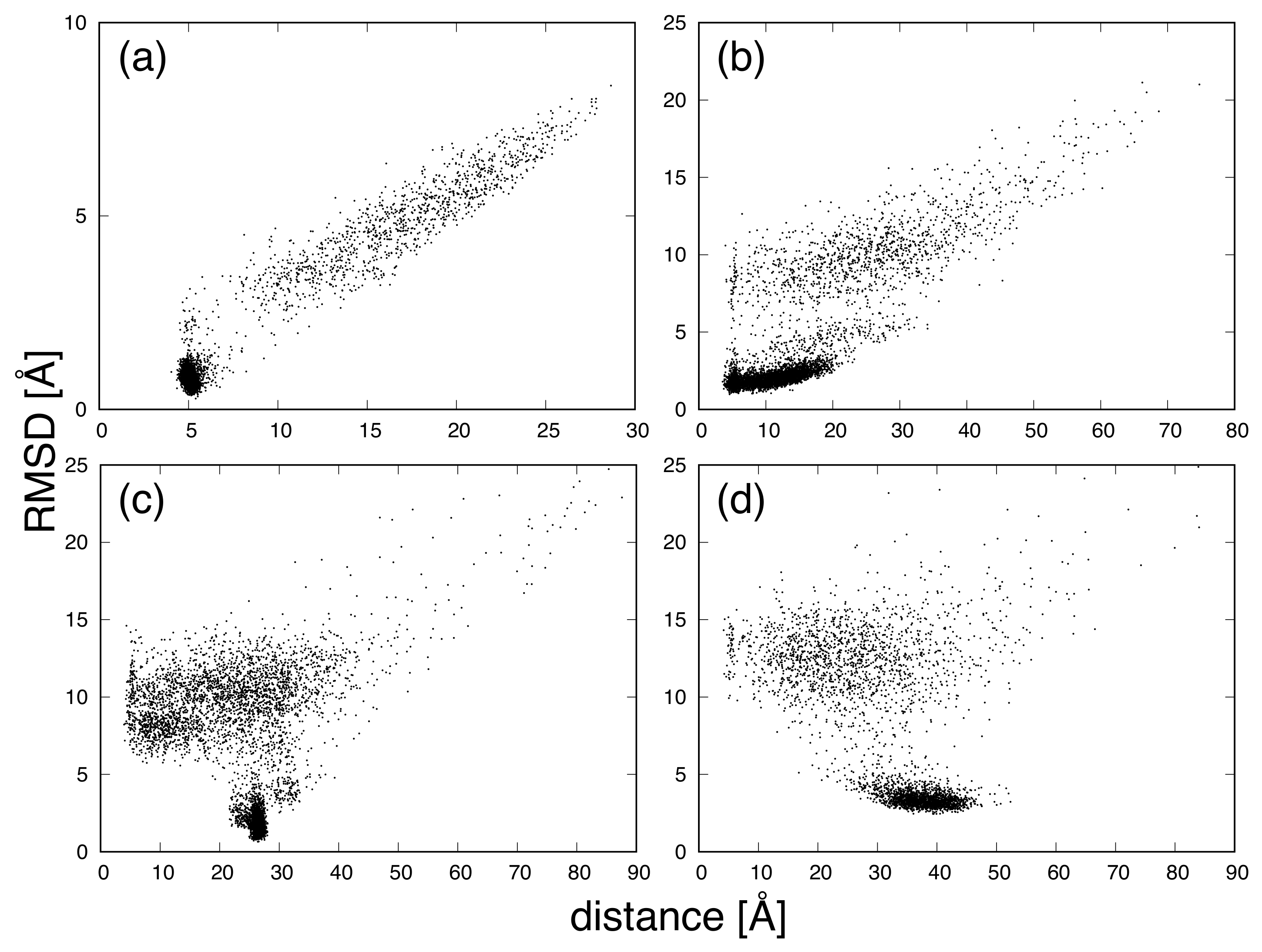
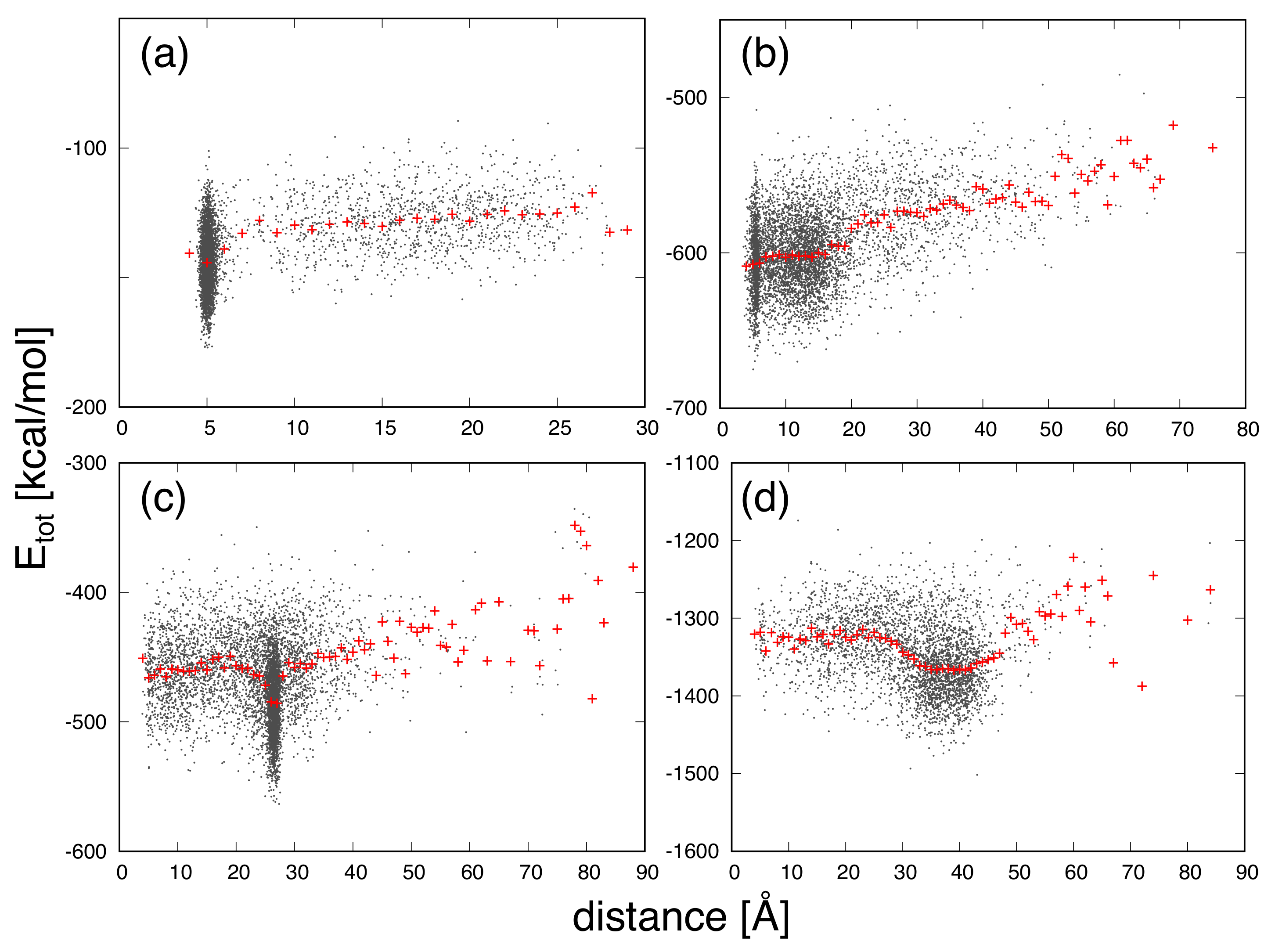
Figure 1. C α -RMSD of (a) CLN025, (b) mGTT, (c) mNuG2, and (d) m α 3D as a function of the radius of gyration.
J 05 00009 g001
Figure 2. Backbone structures with the lowest total energy and the shortest end-to-end distance for (a,b) CLN025, (c,d) mGTT, (e,f) mNuG2, and (g,h) m α 3D. Circles indicate the terminal portions of the protein. Chimera [39] was used to generate the figures.
J 05 00009 g002
Figure 3. The radius of gyration of (a) CLN025, (b) mGTT, (c) mNuG2, and (d) m α 3D as functions of the end-to-end distance.
J 05 00009 g003
Figure 4. C α -RMSD of (a) CLN025, (b) mGTT, (c) mNuG2, and (d) m α 3D as functions of the end-to-end distance.
J 05 00009 g004
Figure 5. Total energy ( E tot ) of (a) CLN025, (b) mGTT, (c) mNuG2, and (d) m α 3D as a function of the end-to-end distance. A red point represents the average value for each width 1 Å.
J 05 00009 g005
Figure 6. Conformational energy ( E conf ) of (a) CLN025, (b) mGTT, (c) mNuG2, and (d) m α 3D as a function of the end-to-end distance. A red point represents the average value for each width of 1 Å.
J 05 00009 g006
Figure 7. Solvation free energy ( E sol ) of (a) CLN025, (b) mGTT, (c) mNuG2, and (d) m α 3D as a function of the end-to-end distance. A red point represents the average value for each width of 1 Å.
J 05 00009 g007
Figure 8. Solvation free energy ( E sol ) of (a) CLN025, (b) mGTT, (c) mNuG2, and (d) m α 3D as a function of temperature. Circles, triangles, crosses, and squares correspond to the end-to-end distance 10, 20, 30, and 40 Å.
J 05 00009 g008
Table 2. C α -RMSD, the end-to-end distance, the radius of gyration (Rg), and the total energy of the lowest-total-energy ( E tot ) and the shortest end-to-end distance (distance) structures for each protein in Figure 2.
ProteinMinimumC α -RMSD [Å]End-to-End Distance [Å]Rg [Å] E tot [kcal/mol]
CLN025 E tot 0.75.06.2−177.0
distance1.04.06.3−136.1
mGTT E tot 1.65.010.1−675.0
distance1.83.610.2−596.0
mNuG2 E tot 1.927.410.7−563.4
distance8.23.911.2−493.9
m α 3D E tot 3.643.113.2−1501.7
distance14.34.212.9−1287.9
Publisher’s Note: MDPI stays neutral with regard to jurisdictional claims in published maps and institutional affiliations.

