Article

Effect of Land Surface Temperature on Urban Heat Island in Varanasi City, India

1
School of Geography, University of Nottingham, Nottingham NG7 2RD, UK
2
Faculty of Engineering, University of Nottingham, Nottingham NG7 2RD, UK
3
Department of Civil Engineering, Indian Institute of Technology Roorkee, Roorkee 247667, India
4
Department of Soil and Water Engineering, Indira Gandhi Krishi Vishwavidyalaya Raipur, Raipur 492012, India
*
Author to whom correspondence should be addressed.
J 2021, 4(3), 420-429; https://doi.org/10.3390/j4030032
Submission received: 3 July 2021 / Revised: 30 July 2021 / Accepted: 3 August 2021 / Published: 6 August 2021
(This article belongs to the Section Environmental Sciences)

Abstract

:
Crucial changes in urban climate can be witnessed due to rapid urbanisation of cities across the world. It is important to find a balance between urban expansion and thermal environment quality to guarantee sustainable urban development. Thus, it is a major research priority to study the urban heat island (UHI) in various fields, i.e., climate change urban ecology, urban climatology, urban planning, mitigation and management, urban geography, etc. The present study highlighted the interrelationship between land surface temperature (LST) and the abundance of impervious cover and green cover in the Varanasi city of Uttar Pradesh, India. For this purpose, we used various GIS and remote-sensing techniques. Landsat 8 images, land-use–land-cover pattern including urban/rural gradients, and grid- and metric-based multi-resolution techniques were used for the analysis. From the study, it was noticed that LST, density of impervious cover, and density of green cover were correlated significantly, and an urban gradient existed over the entire city, depicting a typical UHI profile. It was also concluded that the orientation, randomness, and aggregation of impervious cover and green cover have a strong correlation with LST. From this study, it is recommended that, when planning urban extension, spatial variation of impervious cover and green cover are designed properly to ensure the comfort of all living beings as per the ecological point of view.

1. Introduction

Urban heat islands (UHIs) can be defined as the local rise in temperature because of urban/landscape growth. It is unintentional climate modification when both atmosphere and surfaces in urbanised areas have warmth characteristics compared to their non-urbanised surroundings [1,2]. A major cause of a UHI is the heat generated from urban structures and other heat sources when they consume and re-radiate solar radiations [3,4]. These are caused by anthropogenic activities, population outbursts, elevated emissions, air pollution, thermal power plants, greenhouse gas emissions, energy consumption, and so on [1,5,6]. UHI can cause major problems such as the worsening of living surroundings [7], increment of energy expenditure [8], elevation of ground-level ozone [9], increase in diseases and death rates [10], and negative impact on the ecosystem and climate change [11]. The urban population is forecasted to be 5 billion by 2030 [12], and cities with a large population and extensive urban fabric are more prone to UHI-related problems [13].
The concept of the UHI was first proposed in the year 1818 by Luke Howard [14] when research conducted in urban areas concluded that the atmospheric and surface temperature increased significantly in urban landscapes as compared to the surrounding areas. UHIs can be classified into two types: atmospheric UHI (AUHI) and surface UHI (SUHI). AUHIs are assessed using air temperature, while SUHIs are assessed using land surface temperature (LST) [5].
The literature highlights that remote-sensing- and GIS-based techniques are highly efficient to study the interdependency of the urban landscape pattern, LST, and UHIs [1,15,16,17,18,19]. Remote-sensing and GIS techniques provide better accuracy and spatial resolution and are less time-consuming and more economical compared to other traditional methods of monitoring large areas (cities or states) [20]. The technique presented in this study is based on the urban–rural gradient, multi-resolution analysis, and spatial matrix.
In order to reduce LST-related problems, proper town planning should be adopted using heat-absorbing materials, selection of settlement colours, urban green cover, and vegetated landscapes [21,22,23,24,25,26,27,28]. One of the best solutions for reduction of LST is to increase the green cover which acts as thermal resistance because of the evapotranspiration effect and emissivity of space [29,30,31,32,33]. Green cover helps in creating the shelter, and its coverage also prevents direct solar radiation effects over the surface/space [34,35].
Researchers have attempted to study the relationships between the UHI, LST, and spatial variation of impervious cover and green cover in different regions worldwide [15,36,37,38,39]. However, there is a lack of such studies for Indian regions because of heterogeneity in the land-use–land-cover (LULC) pattern. Surface temperature is not only important to study urban climatology, but it is central to the energy balance of surfaces [40]. In addition, surface temperature is correlated with the land use and variability of its spatial patterns [41]. For the purposes of this study, the SUHI was considered to analyse the UHI effect on Varanasi city.
Our study’s emphasis was on zonal variation in landscape composition and its impact on LST–SUHI over Varanasi city. For this purpose, Landsat 8 OLI/TIRS data and multi-grid-resolution-based geo-spatial techniques were used. In this study, SUHIs were based on LST and were identified using daytime images only as LST values are highly influenced by solar radiations [42]. The vegetation density of the urban area was also considered as it directly influences the LST and SUHI phenomenon. LST values are low when the vegetation area is large and vice versa [1]. This study will be helpful in designing cities to minimize SUHI impact so that urban extension can have sustainable and healthier environments. In addition, it will provide civil engineering insight into the interaction between urban surfaces and the environment.
This study aimed to investigate the influencing parameters on the formation of the SUHI and discuss the potential causes of the SUHI. It also demonstrates the applicability of RS and GIS techniques to study the SUHI. Furthermore, surface temperature was tested to determine whether it provides enough information for the estimation of UHI formation. The study investigated the spatial change of the SUHI of Varanasi city using surface temperature and the urban–rural gradient.

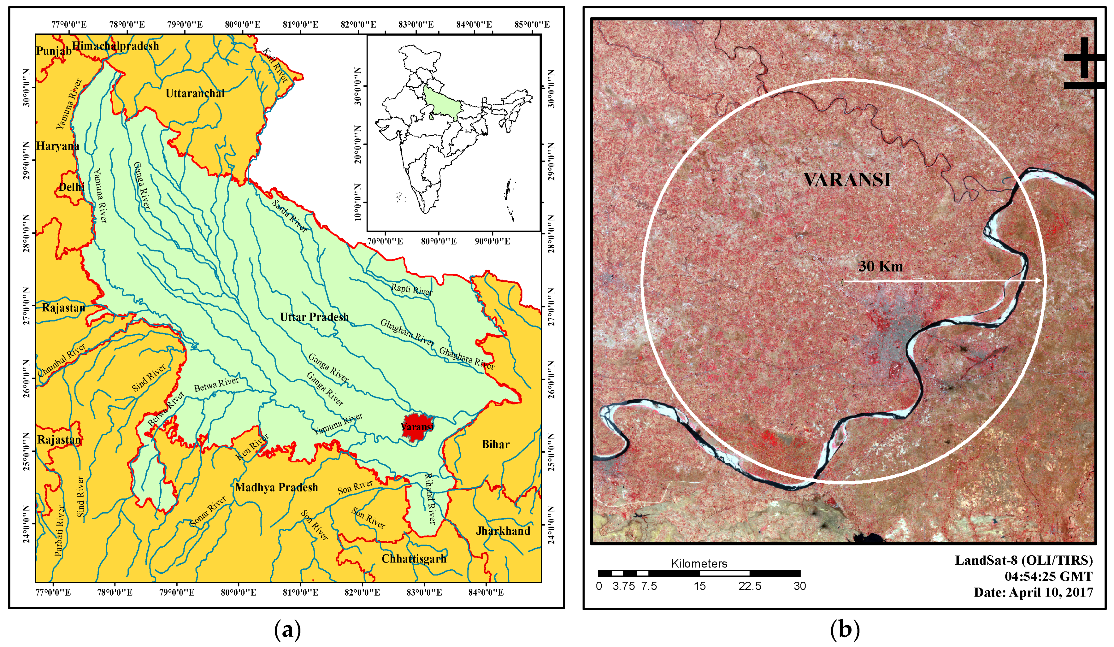
2. Study Area, Data, and Methods

Varanasi, or popularly known as Banaras, is well-known developing city of Uttar Pradesh, India. The city is situated on the banks of the River Ganga (or Ganges) and lies between latitude 25°10′59″ N to 25°33′51″ N and longitude 82°36′23″ E to 83°12′47″ E. The city is popular for its sacredness and its religious importance to the people of India because of holy Ganges. The geographical area of the city is about 1592 km2. The city is surrounded by six districts, namely Jaunpur, Azamgarh, Ghazipur, Chandauli, Mirzapur, and Sant Ravi Das Nagar. The monsoon season extends from June to September. The temperature typically varies between 22 °C and 46 °C [43,44,45]. The location map of study area is shown in Figure 1.
For this study, Landsat 8 Operational Land Imager and Thermal Infrared Sensor (Landsat 8 OLI/TIRS) images were used. The images were acquired from https://earthexplorer.usgs.gov/ (accessed on 30 April 2017) and are shown in Table 1. These images have 11 bands, containing 8 multispectral bands (band 1st–7th and 9th), one panchromatic (band 8th), and two thermal bands (band 10th and 11th). Pre-processing of datasets was performed based on digital number (DN) of multispectral bands using the ArcMap 10.5.

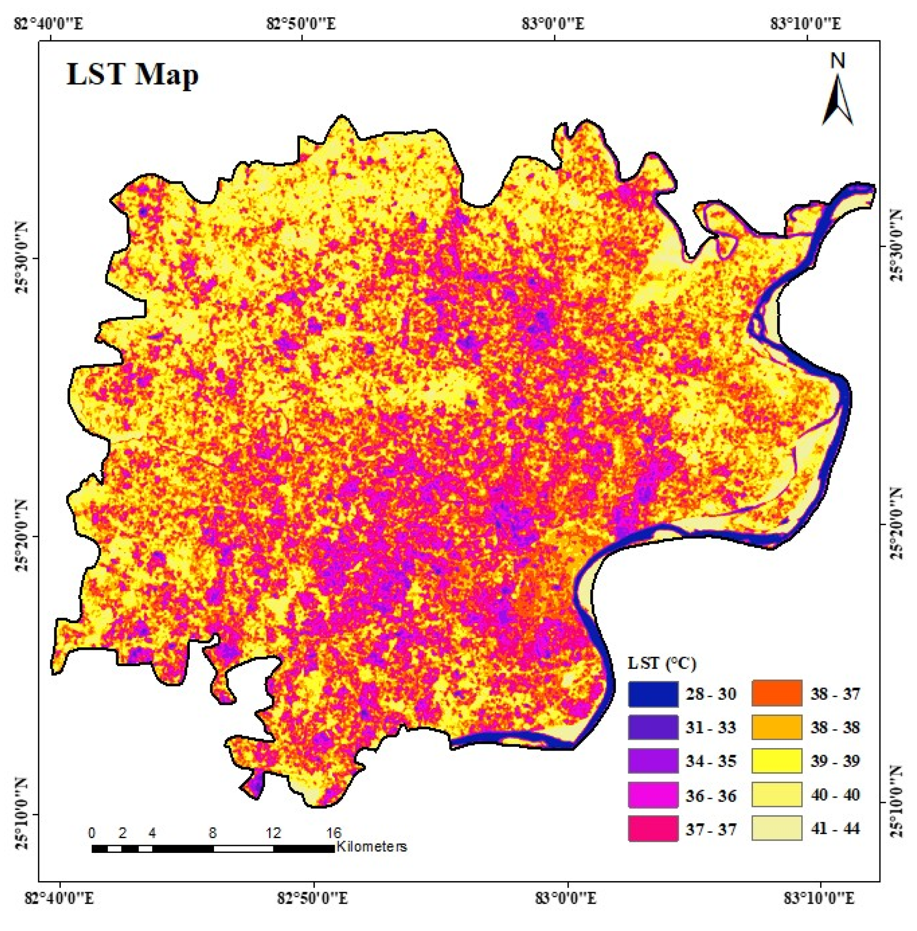
2.1. Calculation of LST

LST calculations from Landsat datasets involved use of DN values of thermal bands and absolute radiance values [46,47]. The datasets were pre-processed to correct pre-launch calibration constants and assumption of unity emissivity of radiance values. In the present study, LST maps were prepared based on 10th band of Landsat 8 imagery. The atmosphere brightness temperature values were provided in Kelvin (K), which were then converted into degrees Celsius (°C, and emissivity-corrected LST was calculated using Equation (1) [15].
L S T ( ° C ) = T B 1 + ( λ × T B ρ ) ln ε
where T B = Landsat 8, 10th band brightness temperature; λ = emitted radiation wavelength (=10.8 μm); ρ = h c σ (1.438 × 10⁻² m·K); σ = Boltzmann constant (1.38 × 10⁻²³ J·K−1); h = Plank’s constant (6.626 × 10⁻³⁴ J·s); c = velocity of light (2.998 × 10⁸ m·s−1); and ε is the land surface emissivity, estimated using Equation (2).
ε = m P v + n
where m = ( ε v ε s ) ( 1 ε s ) F ε v and n = ε s + ( 1 + ε s ) F ε v , where ε v and ε s are the vegetation and soil emissivity, respectively; m (0.004) and n (0.986) value taken from [48]. P v is the vegetation proportion and was obtained using Equation (3).
P v = ( N D V I N D V I m i n N D V I m a x N D V I m i n ) 2
where NDVI is the normalized difference vegetation index [49] given by Equation (4), derived using the surface reflectance of Landsat 8 Bands 4 (Red) and 5 (NIR).
N D V I = ( ρ N I R ρ R e d ) ( ρ N I R + ρ R e d )

2.2. Mapping Topography

For land-cover mapping, Landsat OLI/TIR images were used. We classified the satellite images of the study area into four distinct categories, i.e., water, impervious cover, green cover, and others. A brief description of areas included in each category is shown in Table 2.

2.3. Zonal Spatial Statistical Analysis

For gradient analysis, spatial variation of LST with spatially distributed impervious cover and green cover were analysed. We used statistical buffer-zone technique for gradient calculations; multiple buffer rings were created around the centre of the study area with 300 m offset. For each zone, average LST, impervious-cover density, and green-cover density were determined. Influence of different land-cover categories on LST was examined based on multi-resolution grid polygons with different pixel sizes, viz. 3 × 3, 4 × 4, …, 10 × 10. Average LST, impervious-cover density, and green-cover density were also calculated for each polygon in the study area. We also focused on identifying the prevalent land-cover character, which has influenced the spatial variation of LST in Varanasi district. For this, 60 randomly selected polygon grids from grids sized 10 × 10 pixels were used. Using these randomly selected grid polygons, land-cover map of the study area was clipped and used as an input for this analysis. We used scatter plots and correlation method to establish the relationship between average LST and green-cover density and impervious-cover density for each buffer zone and multi-resolution grids.

3. Results and Discussion

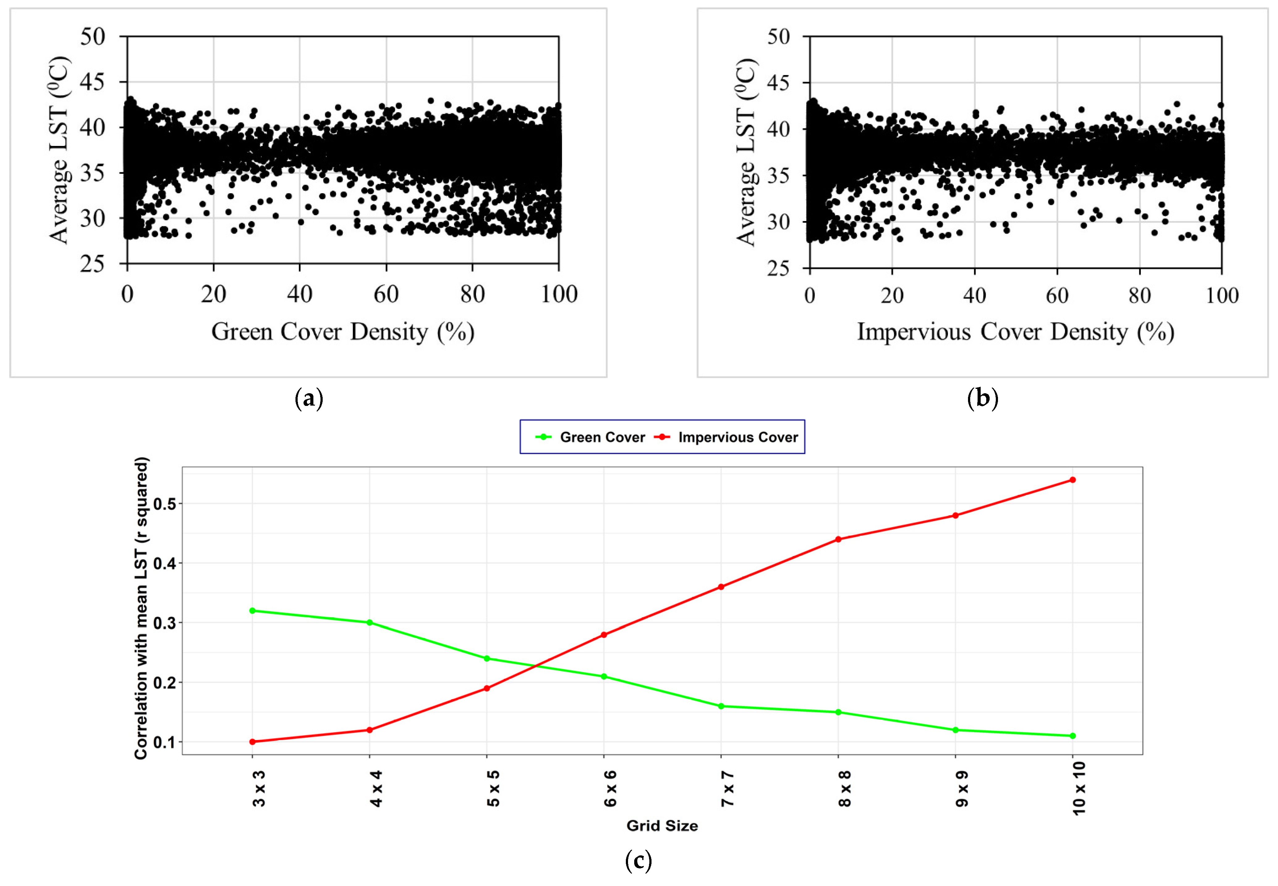
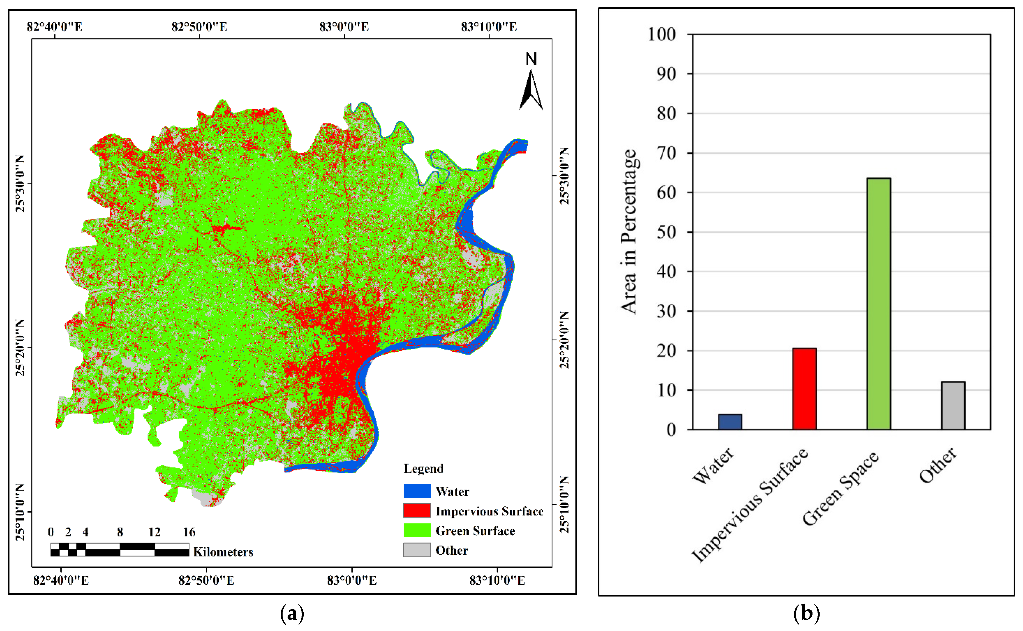
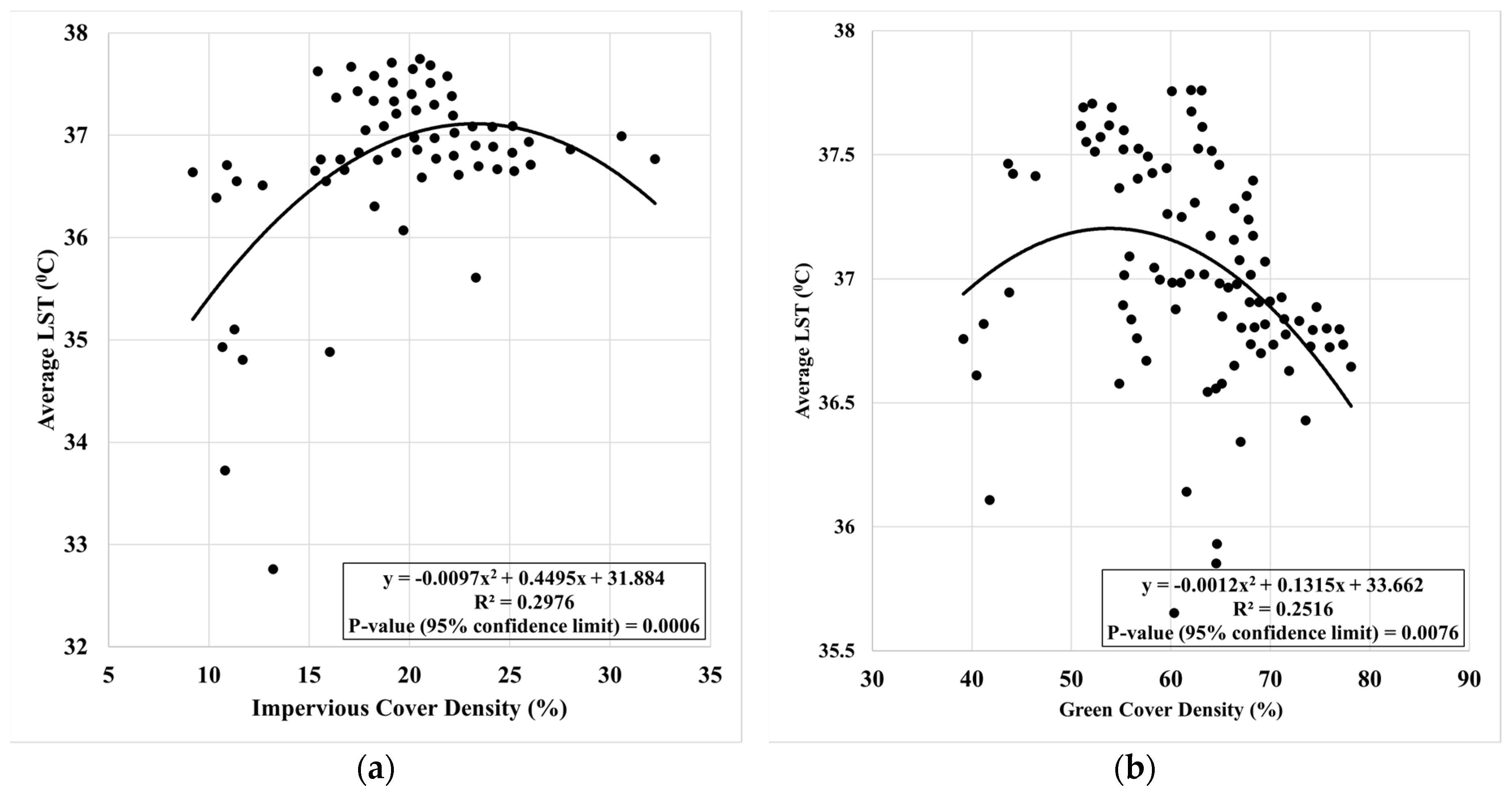
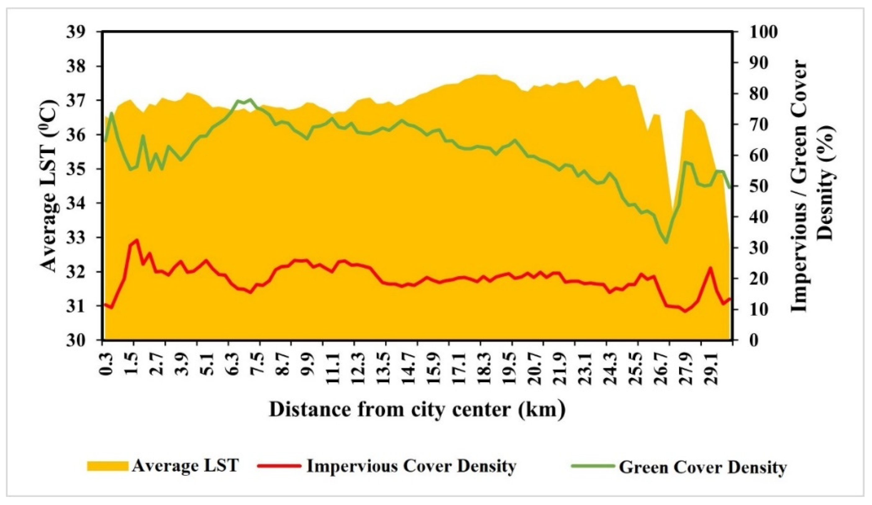
3.1. LST Variation with Changing Land Cover

The LULC classification of Landsat 8 (OLI/TIRS) image was carried out using a supervised classification technique as shown in Figure 2. Classification results show a mixture of impervious cover and green cover. Overall, most land is covered by green cover (63.5%), followed by impervious cover (20.6%), others (12.1%), and water (3.8%). However, a higher concentration of impervious cover exists near the centre of the city, with an observed increase in green-cover coverage moving away from the centre.
The land surface temperature (LST) map for Varanasi city is shown in Figure 3. The LST values for the region range from about 28 °C for water surfaces to 44 °C for impervious cover with a mean and standard deviation of 38.2 °C and 11.4 °C, respectively. The difference between average LST over impervious cover (39 °C) and green cover (37.8 °C) was observed to be 1.2 °C. This implies that land-cover change influences land surface temperature. These findings highlight the potential of classified urban cover based on training classes (LULC categories) and indices using RS data (LST) and are consistent with the results in connection to the SUHI effect in Bangkok, Jakarta, and Manila cities of Southeast Asia [15].

3.2. LST Variation with Changing Land Use

Both the impervious cover and average LST values were observed to gradually decrease along the urban–rural gradient (i.e., gradual decrease from urban towards rural area), whereas green-cover density showed a contrasting pattern. However, the relationship between the density of green cover and average LST was comparatively weaker compared to the impervious-cover densities and average LST (Figure 4). For a range of 10% to 20% of impervious-cover density, average LST ranged from 32 °C to 37 °C, while for areas having an impervious-cover-density range of 20% to 40%, the variation in average LST was low ranging from 36 °C to 38 °C. With the increase in green-cover density, a decline in average LST was observed. Figure 4 shows that for impervious cover, small changes in cover density have a comparatively greater impact on average LST than for green cover.
The results highlight that the average LST increases gradually, reaching its maxima at approximately 19 km from the centre of the city (Figure 5). This may be due to the fact that up to 19 km from the centre, green-cover density decreases gradually and impervious-cover density remains almost constant with few spikes and troughs. Considering a comparatively stronger relationship between impervious-cover density and average LST, a consistent model exists among the average LST values and impervious-cover density along the urban–rural gradient. This reflects a distinctive SUHI profile, where LST reduces along the urban–rural gradient. The results also show a sudden drop in impervious-cover density along the urban–rural gradient with a subsequent drop in LST from a zone of 25.5 km to 29 km, which further highlights the effect of impervious cover on LST. Hence, we recommend city planners and policy makers take necessary measures to increase green-cover density in zones with high LST such as the construction of green rooftops, tree planting, growing urban gardens, and similar other measures [50].

3.3. Multi-Resolution LST Variation with Changing LULC

Figure 6a,b shows the results of correlation coefficients between impervious-cover density, green-cover density, and average LST for various grid sizes. An increasing trend was observed in the correlation between impervious-cover density and average LST with an increasing size of grids. This increasing trend shows that large areas strongly influence the impervious cover on the average LST values. The results are coherent with a few other works available using a similar approach [15,51,52,53,54].
On the contrary, the correlation between green-cover density and average LST decreases as the size of the grid increases and thus represents a weaker influence of green-cover density in larger areas. Generally, areas nearby to green cover witness its cooling effect, which explains the above-observed trend in correlation values of green-cover density and LST values. However, the magnitude of the correlation between green cover and average LST gets constant at and beyond the grid size of 8 × 8 (Figure 6b). This dimension size is important as it can be considered as an optimal threshold area for establishing relationships between surface/air temperatures and LULC characteristics in order to simulate or predict meteorological or environmental parameters within the region [15].

4. Conclusions

The interrelation between LST, SUHI abundance, and spatial distribution of impervious cover and green cover of Varanasi city was highlighted in this study. Landsat 8 OLI/TIRS data were used, and the analysis was conducted on the basis of the urban/settlement gradient, multi-resolution grid, and spatial metrics approach. A relationship was observed between average LST and impervious-cover density along urban/settlement gradients of the Varanasi city. In addition, a relationship was studied between average LST and green-cover density along urban/settlement gradients of the Varanasi city. A typical SUHI profile was observed where the correlation between average LST and density of impervious cover increased in larger grids as compared to the correlation between average LST and density of green cover. Thus, LST variation is influenced by impervious and green cover in bigger and smaller areas, respectively. It was also noticed that the orientation, complexity, and aggregation of impervious cover and green cover highly influence average LST. The study can be helpful for sustainable LULC planning and mitigation under consideration of climate change. It demonstrates the use of available free remotely sensed GIS data to enhance the spatial resolution of SUHI visual and statistical models. It also highlights the surrounding climatic variability, meteorology, and ecological aspects of the study area. We recommend city designers and policy-making bodies must consider the area within 0.3 km to 6 km from the centre of the city seriously as green cover is low and average LST is high in this zone.

Author Contributions

Conceptualization, A.K., V.A., L.P., S.K.C. and V.M.; Data curation, A.K., L.P. and S.K.C.; Formal analysis, A.K., V.A., L.P., S.K.C. and V.M.; Funding acquisition, V.A.; Investigation, L.P. and S.K.C.; Methodology, A.K., V.A., L.P., S.K.C. and V.M.; Software, A.K., V.A. and L.P.; Visualization, L.P. and V.M.; Writing—original draft, A.K. and S.K.C.; Writing—review and editing, A.K., V.A. and S.K.C. All authors have read and agreed to the published version of the manuscript.

Funding

This research received no external funding.

Acknowledgments

The authors would like to acknowledge the lab facilities provided by the University of Nottingham (UK), the Indian Institute of Technology Roorkee (India), and the National Institute of Hydrology Roorkee (India).

Conflicts of Interest

The authors declare no conflict of interest.

References

  1. Voogt, J.A. Urban heat islands: Hotter cities. Am. Inst. Biol. Sci. 2004. Available online: https://www.populationenvironmentresearch.org/node/9316 (accessed on 14 June 2021).
  2. Aboelata, A.; Sodoudi, S. Evaluating the effect of trees on UHI mitigation and reduction of energy usage in different built up areas in Cairo. Build. Environ. 2020, 168, 106490. [Google Scholar] [CrossRef]
  3. O’Malley, C.; Piroozfar, P.; Farr, E.R.P.; Pomponi, F. Urban Heat Island (UHI) mitigating strategies: A case-based comparative analysis. Sustain. Cities Soc. 2015, 19, 222–235. [Google Scholar] [CrossRef] [Green Version]
  4. Sun, T.; Sun, R.; Chen, L. The trend inconsistency between land surface temperature and near surface air temperature in assessing urban heat island effects. Remote Sens. 2020, 12, 1271. [Google Scholar] [CrossRef] [Green Version]
  5. US EPA. Chapter 5: Cool Pavements. In Reducing Urban Heat Islands: Compendium of Strategies; US EPA: Washington, DC, USA, 2008. [Google Scholar]
  6. Shukla, A.; Jain, K. Analyzing the impact of changing landscape pattern and dynamics on land surface temperature in Lucknow city, India. Urban For. Urban Green. 2021, 58, 126877. [Google Scholar] [CrossRef]
  7. Heaviside, C.; Macintyre, H.; Vardoulakis, S. The urban heat island: Implications for health in a changing environment. Curr. Environ. Health Rep. 2017, 4, 296–305. [Google Scholar] [CrossRef]
  8. Konopacki, S.; Akbari, H. Energy Savings of Heat-Island Reduction Strategies in Chicago and Houston (Including Updates for Baton Rouge, Sacramento, and Salt Lake City). Energy 2002. LBNL-49638 Lawrence Berkeley National Laboratory. Available online: https://escholarship.org/uc/item/2rv7n2gn (accessed on 2 August 2021).
  9. Rosenfeld, A.H.; Akbari, H.; Romm, J.J.; Pomerantz, M. Cool communities: Strategies for heat island mitigation and smog reduction. Energy Build. 1998, 28, 51–62. [Google Scholar] [CrossRef]
  10. Changnon, S.A.; Kunkel, K.E.; Reinke, B.C. Impacts and responses to the 1995 heat wave: A call to action. Bull. Am. Meteorol. Soc. 1996, 77, 1497–1506. [Google Scholar] [CrossRef] [Green Version]
  11. Yu, Z.; Jing, Y.; Yang, G.; Sun, R. A new urban functional zone-based climate zoning system for urban temperature study. Remote Sens. 2021, 13, 251. [Google Scholar] [CrossRef]
  12. Nations United. Nations Nations (UN) Goals. 2021. Available online: https://sdgs.un.org/goals (accessed on 21 June 2021).
  13. Chen, M.; Zhou, Y.; Hu, M.; Zhou, Y. Influence of Urban Scale and Urban Expansion on the Urban Heat Island Effect in Metropolitan Areas: Case Study of Beijing-Tianjin-Hebei Urban Agglomeration. Remote Sens. 2020, 12, 3491. [Google Scholar] [CrossRef]
  14. Howard, L. The Climate of London: Deduced from Meteorological Observations, Made at Different Places in the Neighbourhood of the Metropolis; Cambridge University Press: Cambridge, UK, 1818; Volume 1. [Google Scholar]
  15. Estoque, R.C.; Murayama, Y.; Myint, S.W. Effects of landscape composition and pattern on land surface temperature: An urban heat island study in the megacities of Southeast Asia. Sci. Total Environ. 2017, 577, 347–359. [Google Scholar] [CrossRef]
  16. Kim, H.H. Urban heat island. Int. J. Remote Sens. 1992, 13, 2319–2336. [Google Scholar] [CrossRef]
  17. Oke, T.R. The energetic basis of the urban heat island. Q. J. R. Meteorol. Soc. 1982, 108, 1–24. [Google Scholar] [CrossRef]
  18. Weng, Q.; Lu, D.; Schubring, J. Estimation of land surface temperature-vegetation abundance relationship for urban heat island studies. Remote Sens. Environ. 2004, 89, 467–483. [Google Scholar] [CrossRef]
  19. Yuan, F.; Bauer, M.E. Comparison of impervious surface area and normalized difference vegetation index as indicators of surface urban heat island effects in Landsat imagery. Remote Sens. Environ. 2007, 106, 375–386. [Google Scholar] [CrossRef]
  20. Agarwal, V.; Kumar, A.; Gomes, R.L.; Marsh, S. Monitoring of ground movement and groundwater changes in London using InSAR and GRACE. Appl. Sci. 2020, 10, 8599. [Google Scholar] [CrossRef]
  21. He, B.-J.; Zhao, Z.-Q.; Shen, L.-D.; Wang, H.-B.; Li, L.-G. An approach to examining performances of cool/hot sources in mitigating/enhancing land surface temperature under different temperature backgrounds based on landsat 8 image. Sustain. Cities Soc. 2019, 44, 416–427. [Google Scholar] [CrossRef]
  22. Song, Y.; Song, X.; Shao, G. Effects of Green Space Patterns on Urban Thermal Environment at Multiple Spatial—Temporal Scales. Sustainability 2020, 12, 6850. [Google Scholar] [CrossRef]
  23. Becker, F. The impact of spectral emissivity on the measurement of land surface temperature from a satellite. Int. J. Remote Sens. 1987, 8, 1509–1522. [Google Scholar] [CrossRef]
  24. Dash, P.; Göttsche, F.M.; Olesen, F.S.; Fischer, H. Land surface temperature and emissivity estimation from passive sensor data: Theory and practice-current trends. Int. J. Remote Sens. 2002, 23, 2563–2594. [Google Scholar] [CrossRef]
  25. Hoag, H. How cities can beat the heat. Nature 2015, 524, 402–404. [Google Scholar] [CrossRef] [PubMed] [Green Version]
  26. Lee, S.; Ryu, Y.; Jiang, C. Urban heat mitigation by roof surface materials during the East Asian summer monsoon. Environ. Res. Lett. 2015, 10, 124012. [Google Scholar] [CrossRef]
  27. Snyder, W.C.; Wan, Z.; Zhang, Y.; Feng, Y.Z. Classification-based emissivity for land surface temperature measurement from space. Int. J. Remote Sens. 1998, 19, 2753–2774. [Google Scholar] [CrossRef]
  28. Vancutsem, C.; Ceccato, P.; Dinku, T.; Connor, S.J. Evaluation of MODIS land surface temperature data to estimate air temperature in different ecosystems over Africa. Remote Sens. Environ. 2010, 114, 449–465. [Google Scholar] [CrossRef]
  29. Li, X.; Zhou, W.; Ouyang, Z. Relationship between land surface temperature and spatial pattern of greenspace: What are the effects of spatial resolution? Landsc. Urban Plan. 2013, 114, 1–8. [Google Scholar] [CrossRef]
  30. Guo, G.; Wu, Z.; Cao, Z.; Chen, Y.; Zheng, Z. Location of greenspace matters: A new approach to investigating the effect of the greenspace spatial pattern on urban heat environment. Landsc. Ecol. 2021, 36, 1533–1548. [Google Scholar] [CrossRef]
  31. Yuan, B.; Zhou, L.; Dang, X.; Sun, D.; Hu, F.; Mu, H. Separate and combined effects of 3D building features and urban green space on land surface temperature. J. Environ. Manag. 2021, 295, 113116. [Google Scholar] [CrossRef]
  32. Connors, J.P.; Galletti, C.S.; Chow, W.T.L. Landscape configuration and urban heat island effects: Assessing the relationship between landscape characteristics and land surface temperature in Phoenix, Arizona. Landsc. Ecol. 2013, 28, 271–283. [Google Scholar] [CrossRef]
  33. Maimaitiyiming, M.; Ghulam, A.; Tiyip, T.; Pla, F.; Latorre-Carmona, P.; Halik, Ü.; Sawut, M.; Caetano, M. Effects of green space spatial pattern on land surface temperature: Implications for sustainable urban planning and climate change adaptation. ISPRS J. Photogramm. Remote Sens. 2014, 89, 59–66. [Google Scholar] [CrossRef] [Green Version]
  34. Streutker, D.R. Satellite-measured growth of the urban heat island of Houston, Texas. Remote Sens. Environ. 2003, 85, 282–289. [Google Scholar] [CrossRef]
  35. Shukla, A.; Jain, K. Critical analysis of rural-urban transitions and transformations in Lucknow city, India. Remote Sens. Appl. Soc. Environ. 2019, 13, 445–456. [Google Scholar] [CrossRef]
  36. Zhou, D.; Zhang, L.; Hao, L.; Sun, G.; Liu, Y.; Zhu, C. Spatiotemporal trends of urban heat island effect along the urban development intensity gradient in China. Sci. Total Environ. 2016, 544, 617–626. [Google Scholar] [CrossRef]
  37. Priyadarshini, K.N.; Sivashankari, V.; Shekhar, S.; Balasubramani, K. Examining Land Surface Temperature from Agglomerative Spectra Using Hyperspectral Dataset. Sustain. Clim. Action Water Manag. 2021, 203–209. [Google Scholar] [CrossRef]
  38. Roy, S.; Pandit, S.; Eva, E.A.; Bagmar, M.S.H.; Papia, M.; Banik, L.; Dube, T.; Rahman, F.; Razi, M.A. Examining the nexus between land surface temperature and urban growth in Chattogram Metropolitan Area of Bangladesh using long term Landsat series data. Urban Clim. 2020, 32, 100593. [Google Scholar] [CrossRef]
  39. Rihan, M.; Naikoo, M.W.; Ali, M.A.; Usmani, T.M.; Rahman, A. Urban Heat Island Dynamics in Response to Land-Use/Land-Cover Change in the Coastal City of Mumbai. J. Indian Soc. Remote Sens. 2021, 1–21. [Google Scholar] [CrossRef]
  40. Oke, T.R.; Spronken-Smith, R.A.; Jáuregui, E.; Grimmond, C.S.B. The energy balance of central Mexico City during the dry season. Atmos. Environ. 1999, 33, 3919–3930. [Google Scholar] [CrossRef]
  41. Balling, R.C. High-resolution surface temperature patterns in a complex urban terrain. Photogramm. Eng. Remote Sens. 1988, 54, 1289–1293. [Google Scholar]
  42. Leconte, F.; Bouyer, J.; Claverie, R.; Pétrissans, M. Using Local Climate Zone scheme for UHI assessment: Evaluation of the method using mobile measurements. Build. Environ. 2015, 83, 39–49. [Google Scholar] [CrossRef]
  43. Pratap, V.; Saha, U.; Kumar, A.; Singh, A.K. Analysis of air pollution in the atmosphere due to firecrackers in the Diwali period over an urban Indian region. Adv. Sp. Res. 2021. [Google Scholar] [CrossRef]
  44. Adinehvand, M.; Singh, B.N. Prediction of climate change scenarios in Varanasi District, UP, India, using simulation models. Mausam 2021, 72, 313–322. [Google Scholar]
  45. Singh, N.; Mhawish, A.; Ghosh, S.; Banerjee, T.; Mall, R.K. Attributing mortality from temperature extremes: A time series analysis in Varanasi, India. Sci. Total Environ. 2019, 665, 453–464. [Google Scholar] [CrossRef]
  46. Jiménez-Muñoz, J.C.; Sobrino, J.A.; Skoković, D.; Mattar, C.; Cristóbal, J. Land surface temperature retrieval methods from Landsat-8 thermal infrared sensor data. IEEE Geosci. Remote Sens. Lett. 2014, 11, 1840–1843. [Google Scholar] [CrossRef]
  47. Ru, C.; Duan, S.-B.; Jiang, X.-G.; Li, Z.-L.; Jiang, Y.; Ren, H.; Leng, P.; Gao, M. Land Surface Temperature Retrieval From Landsat 8 Thermal Infrared Data Over Urban Areas Considering Geometry Effect: Method and Application. IEEE Trans. Geosci. Remote Sens. 2021, 1–66. [Google Scholar] [CrossRef]
  48. Sobrino, J.A.; Jiménez-Muñoz, J.C.; Paolini, L. Land surface temperature retrieval from LANDSAT TM 5. Remote Sens. Environ. 2004, 90, 434–440. [Google Scholar] [CrossRef]
  49. Rouse, J.W.; Hass, R.H.; Schell, J.A.; Deering, D.W.; Harlan, J.C. Monitoring the Vernal Advancement and Retrogradation (Green Wave Effect) of Natural Vegetation; Final Report RSC 1978-4; Texas A&M University: College Station, TX, USA, 1974. [Google Scholar]
  50. Yang, J.; Wang, Y.; Xiu, C.; Xiao, X.; Xia, J.; Jin, C. Optimizing local climate zones to mitigate urban heat island effect in human settlements. J. Clean. Prod. 2020, 275, 123767. [Google Scholar] [CrossRef]
  51. Talukdar, S.; Rihan, M.; Hang, H.T.; Bhaskaran, S.; Rahman, A. Modelling urban heat island (UHI) and thermal field variation and their relationship with land use indices over Delhi and Mumbai metro cities. Environ. Dev. Sustain. 2021, 1–29. [Google Scholar] [CrossRef]
  52. Wu, Z.; Zhang, Y. Spatial variation of urban thermal environment and its relation to green space patterns: Implication to sustainable landscape planning. Sustainability 2018, 10, 2249. [Google Scholar] [CrossRef] [Green Version]
  53. Anguluri, R.; Narayanan, P. Role of green space in urban planning: Outlook towards smart cities. Urban For. Urban Green. 2017, 25, 58–65. [Google Scholar] [CrossRef]
  54. Sun, R.; Chen, L. Effects of green space dynamics on urban heat islands: Mitigation and diversification. Ecosyst. Serv. 2017, 23, 38–46. [Google Scholar] [CrossRef]
Figure 1. (a) Location map of Varanasi city, India (study area). (b) White circle shows Varanasi city marked on Landsat 8. image.
J 04 00032 g001
Figure 2. (a) Land-use–land-cover (LULC)-classified map of Varanasi city. (b) Percentage-area-based division of the four LULC categories.
J 04 00032 g002
Figure 3. Land surface temperature (LST) map of Varanasi city developed using Landsat 8 imagery.
J 04 00032 g003
Figure 4. Correlation plots between average LST along urban rural gradient and (a) impervious cover density and (b) green cover density.
J 04 00032 g004
Figure 5. Variation of actual average land surface temperature (LST) and impervious and green cover density along urban rural gradient.
J 04 00032 g005
Figure 6. Scatter plots between average land surface temperature (LST) and (a) green cover density and (b) impervious cover density. (c) Variation in correlation of average LST and impervious and green cover density against variation in resolution.
J 04 00032 g006
Table 1. Description of Landsat 8 image acquisition for Varanasi city.
CityLandsat 8 Scene IDAcquisition Date and Time (GMT)Season
Varanasi CityLC81420422017100LGN0010 April 2017; 04:54:25Dry
LC81420432017100LGN0010 April 2017; 04:54:49Dry
Table 2. Description of land-use–land-cover (LULC) categories considered for the classification of study area.
CategoryDescription
WaterAll water-covered areas (e.g., sea, lake, river, and ponds).
Impervious coverAll impervious cover (e.g., buildings, roads, airports, parking area, and tennis courts)
Green coverAll vegetation covers (e.g., forest and grass)
OthersAll land cover except water, impervious cover, and green cover
Publisher’s Note: MDPI stays neutral with regard to jurisdictional claims in published maps and institutional affiliations.

