Abstract
The overlapping problem occurs when a region of the dimensional data space is shared in a similar proportion by different classes. It has an impact on a classifier’s performance due to the difficulty in correctly separating the classes. Further, an imbalanced dataset consists of a situation in which one class has more instances than another, and this is another aspect that impacts a classifier’s performance. In general, these two problems are treated separately. On the other hand, Prototype Selection (PS) approaches are employed as strategies for selecting appropriate instances from a dataset by filtering redundant and noise data, which can cause misclassification performance. In this paper, we introduce Filtering-based Instance Selection (FIS), using as a base the Self-Organizing Maps Neural Network (SOM) and information entropy. In this sense, SOM is trained with a dataset, and, then, the instances of the training set are mapped to the nearest prototype (SOM neurons). An analysis with entropy is conducted in each prototype region. From a threshold, we propose three decision methods: filtering the majority class (H-FIS (High Filter IS)), the minority class (L-FIS (Low Filter IS)), and both classes (B-FIS). The experiments using artificial and real dataset showed that the methods proposed in combination with 1NN improved the accuracy, F-Score, and G-mean values when compared with the 1NN classifier without the filter methods. The FIS approach is also compatible with the approaches mentioned in the relevant literature.
1. Introduction
A situation that can cause problems in the performance of a classifier is class overlapping. It occurs when a region of the dimensional data space is shared in a similar proportion by different classes, resulting in misclassification.
In addition to the problems that impact a classifier’s performance, an imbalanced dataset is a rather common problem that appears in different areas of knowledge such as medicine, psychology, industry, and in some other areas [1,2,3,4]. The imbalance problem comprises a situation in which one of the classes (i.e., the majority class) has more instances than the other class (i.e., the minority class).
Studies on this subject indicate that the overlapping of data can have a greater impact in terms of loss of accuracy than an imbalance of classes [5,6,7]. In the relevant literature, most of the works deal with these problems separately.
The classical algorithms to minimize class overlapping are defined as follows: Edited Nearest Neighbor (ENN), which removes the instance with the class that disagrees with neighborhood classes [8]; Decremental Reduction Optimization Procedure 3 (DROP3), a classification process the is conducted and the misclassification instances are removed [8]; Adaptive Threshold-based Instance Selection Algorithm 1 (ATISA1), which is similar to DROP3 with the difference that the instance classified as correct is selected [9]; and Ranking-based Instance Selection (RIS), which is a ranking-based approach defined by the relation of neighbor instance classes [10].
The class imbalance problems can be defined into data-level approaches and algorithmic-level approaches [11,12]. Data-level approaches consist of a sampling dataset realized, in a random way, with the objective of an undersampling or oversampling dataset. Algorithm-level approaches consist of an ensemble of classification algorithms trained with different dataset samples.
However, more recent work has started to address these two problems in a unique way. Vuttipittayamongkol and Elyan proposed an overlap-based undersampling method for maximizing the visibility of the minority class instances in the overlapping region [1]. Elyan et al. proposed a hybrid approach aimed at reducing the dominance of the majority class instances using class decomposition and by increasing the minority class instances using an oversampling method [2]. Yuan et al. proposed a Density-Based Adaptive k-Nearest Neighbors method (DBANN), which can handle imbalance- and overlapping-related problems simultaneously. To do so, a simple but effective distance adjustment strategy has been developed to adaptively find the most reliable query neighbors [4].
One classifier that is especially vulnerable to the overlapping problem and imbalanced dataset is the supervised method of Instance-Based Learning (IBL) [6]. The kNN classifier is a traditional IBL algorithm, which works using the nearest neighbor approach to classify an instance [13].
Several strategies have been proposed to solve these issues for kNN. One of these strategies is to use data reduction to select instances to enhance the classification process. PS, as this method is called, is similar to a pre-processing step before algorithm training that focuses on selection of instances that can contribute to improving the classification performance and reducing the training (or comparative) timing.
Different methods for this approach have been proposed. Garcia et al. organized all these works in a taxonomy and compared the different methods that try to improve the classification and performance with special reference to kNN [14].
There are different strategies to define the subset of prototypes selected in PS. From among the techniques available in the relevant literature, it is possible to highlight the random methods, distance methods, and clustering and evolutionary algorithms [15].
This work considers the clustering techniques as it evaluates the use of Kohonen’s SOM [16]. SOM is an unsupervised method that clusters the instances according to their similarities. The standard version of this algorithm arranges the instances, according to their Euclidean distance, inside nodes (neurons) that are arranged in the form of a grid. This creates a map of nodes where the instances that are most similar to each other are inside the same node or in neighboring nodes.
The objective of this paper is to propose FIS uses of information entropy that are measured from the data clustered in the SOM’s nodes by using a PS approach. The theory is that, with the removal of the chosen instances, the method will smoothen the borders of difficult datasets such as those suffering from overlap problems by minimizing the imbalanced data [17]. Some papers use SOM to preprocess a dataset [18,19,20]; however, most of them are focused on the generation of another dataset represented by prototypes, which, in the literature, is cited with a deform in the border region, causing the algorithm to reduce the generalization capacity.
In addition to the proposed method, this work has as a contribution the introduction of an overlapped measure to monitor the threshold of entropy, analyzed in each region of SOM nodes to filter the majority class in a region (H-FIS (High Filter IS)), the minority class (L-FIS (Low Filter IS)), and both the classes (B-FIS). These measures were created to identify different attributes that evaluate the data complexity before classification, thus revealing different information about the data, including overlap [21]. For this, a synthetic dataset was created to control the imbalanced dataset and find the best threshold parameters from complexity measures. Finally, this approach was validated using 12 real datasets and contrasting it with 1NN with and without the FIS approach to measure the gain in the data pre-processing.
The rest of the paper is organized as follows. Section 2 provides brief explanations of PS, SOM, and data complexity measures. The methods are proposed in Section 3. The methodology is detailed in Section 4. Experimental results and discussion are presented in Section 5. The last section (Section 6) contains the conclusions.
2. Theoretical Fundamentals
2.1. Prototype Selection
Prototype Selection (PS) consists of an approach to promote a transformation in a dataset by minimizing data complexity, reducing the requirements of storage of the raw dataset, and eliminating instances of noise [14]. The process starts with a raw dataset, and an algorithm of PS is used to find the most representative instance, forming a reduced dataset.
In this regard, suppose a raw dataset is to be used as a training dataset with m attributes and n instances, i.e., , and each instance has a label where . Normally, in the kNN classification process, is used as a model to classify test instances. In the prototype selection, a subset of is selected, i.e., , where . Then, is used to classify the test instances instead of the original .
2.2. Self-Organizing Map
Self-Organizing Map (SOM) is a neural network that organizes a dataset in a grid of neurons located on a regular low-dimensional grid, usually a two-dimensional (2D) one [16]. It is conducted by an unsupervised learning algorithm that aims to associate similar instances in the same neurons or in the adjacent neurons of the grid.
The training set is used to train SOM. Additionally, each neuron j of the SOM grid has a weight vector , where ; here, l is the total number of neurons of SOM.
The learning process starts with a random choice of the training dataset to be compared with the weight vector of the grid that is randomly initialized. The comparison between and is usually made through the Euclidean distance. The shortest distance indicates the closest neuron , which will have its weight vector updated to get close to the selected instance . Formally, neuron is defined in Equation (1):
The closest weights vector and their neighbors are updated using the Kohonen algorithm [16]. However, the topological neighborhood is defined so that the farther away the neuron is from , the lower the intensity of the neighborhood to be updated. Please see the work of Kohonen [16] for a complete explanation of the training rule of the SOM.
2.3. Data Complexity Measures
Data complexity measures can indicate properties of data that increase or reduce the level of performance expected in a process of data classification. Such measures have bee studied by different authors [21,22,23,24,25].
The use of these complexity measures allows a better comprehension of both data distribution in the data space and how classes are separated. In this work too, these measures are used as a tool to gain a better comprehension of the performance of the pre-processing methods in the different datasets and identify the level of data overlap that exists in a dataset.
There are several measures suggested in the relevant literature. It was decided that the works of Cano [24] and Moran [25] would be used. In their different works, these authors identified that F1 and F3 are good measures to identify overlaps for different classifiers, while N2 is a good measure to evaluate the classification performance of kNN. As the works mentioned do not used the D3 measure, we decided to add it to our work.
These measures, described in the following sections, are determined for the two-class problem. For the multi-class problem, it is possible to extend such measures [25].
The Fischer’s Discriminant Ratio (F1) measure [22] calculates the separability between two classes in a determined attribute. The measure for an attribute is given in Equation (2):
where and are the class average measures and and are the respective standard deviations.
In a dataset with m attributes, the measure is calculated for each of these attributes. The value considered as F1 is the greatest value of f, i.e., the attribute with the greatest separation.
Low values of F1 indicate classes with closer data centers, which, in turn, indicate data overlap.
The Maximum (Individual) Feature Efficiency (F3) measure is calculated for each attribute based on their efficacy to separate classes [21]. This measure is calculated using the maximum and minimum values of the attributes in each of the classes. The value is taken as the fraction of instances that are outside the range of the opposite class.
The value of F3 is defined as the greatest value among the attributes. The value of this measure ranges from 0 to 1, where lower values indicate greater overlap.
The Ratio of Average Intraclass/Interclass NN Distance (N2) measure is calculated as the ratio of the intraclass distance to the interclass distance of the instances. This measure shows the distributions of the classes and how close the classes are to each other [21]. This measure is given by Equation (3):
where represents the instances and n represents the total number of instances. Low values of N2 indicate that the classes are more separable and, thus, easier to identify.
The class density in overlap region (D3) measure was proposed by Sanchez [23], and it indicates the number of instances there are in an overlapped area.
For the present purpose, this measure uses a kNN to evaluate whether an instance disagrees with its neighbors. In the case it does, that instance is marked as an overlapped instance. The result of the measure is the fraction of instances that are marked as being overlapped when compared with the total number of instances.
To identify these instances, the value of k must be chosen for the kNN classifier. For this work, the kNN used for the measures had as the original work.
3. Filtering-Based Instance Selection Algorithm
The proposed method is developed on a trained SOM. As the instances with similar attributes are mapped in the same neurons, it is expected that the instances with different classes can co-exist inside the neuron, i.e., overlapped classes.
Thus, after SOM training, a second step is introduced in this paper. This step consists of post-processing through entropy calculation for each neuron of the grid [26]. The Shannon entropy for the two probabilities is defined in Equation (4):
where p is the probability of class A inside the neuron and q of class B, where .
It is important to note that the entropy in the proposed method is calculated only according to the distribution inside each SOM’s node. The overall distribution of the classes has no impact.
Based on the entropy value, there are three different filter methods that can be proposed:
- High Filter (H-FIS): If the neuron entropy is higher than or equal to a certain threshold (ThresholdHigh), the overlapped instances are removed. The premise here is that the overlapped instances do not have relevant information to delimited the borders between the classes.
- Low Filter (L-FIS): If the neuron entropy is lower than or equal to ThresholdLow, the instances from the class with the lower probability are removed. The premise here is that removing those instances from the class that do not agree with the majority class can smoothen the borders between the classes.
- Both (High and Low Filter) (B-FIS): H-FIS and L-FIS are combined through the comparison of ThresholdHigh higher than ThresholdLow. The premise here is that instances overlapped in the border can be removed.
After the instance filtering is done using any of the proposed approaches, the selected dataset is defined. This selected dataset () is used for the training of the classification algorithm.
An illustration of the FIS approach is represented in Figure 1. In this example, a hypothetical SOM trained has the instances mapped to the neurons grid. These instances belong to two classes (A and B), where class A is represented by squares and class B by triangles. The instances to be removed are highlighted in the figure.
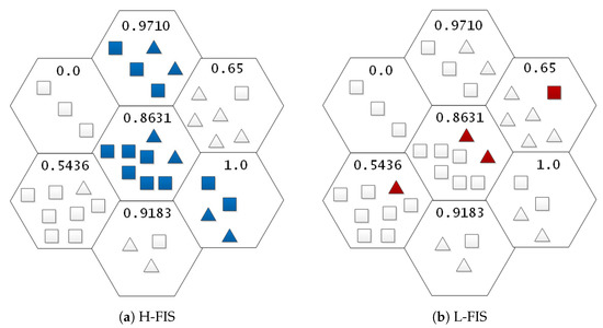
Figure 1.
Example of the selection process to decide which instances should be removed in a hypothetical dataset after the use of SOM using H-FIS (a) and L-FIS (b). The value of the threshold hyperparameter was set at 0.8631 for both H-FIS and L-FIS. The instances selected for removal in this scenario are highlighted.
Figure 1a has the H-FIS approach parameterized with a ThresholdHigh of 0.8631. It is to be noted that the instances removed are in regions where the neuron entropy is equal or higher than the threshold value, and the instances from both the classes are removed. Figure 1b has the L-FIS approach parameterized with a ThresholdLow of 0.8631. Thus, the instances that belong to the minority (highlighted instances) class are removed.
4. Materials and Methods
Figure 2 represents the methodology followed during the experiments involving the FIS approach. In each dataset, an experimental step was considered, as explained in this section.
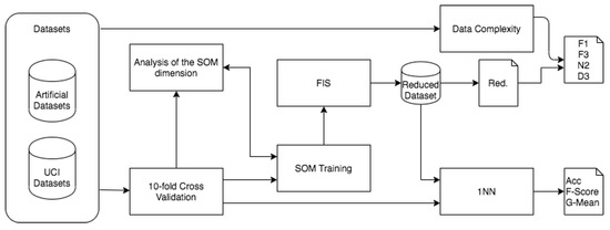
Figure 2.
Schema of experimental methodology.
For the first step, a controlled environment was created to study the effectiveness of the methods in the overlapping problems and in imbalanced datasets.
This environment consists of 121 artificial datasets that represent different levels of overlapped and imbalanced classes. A sample of the dataset is presented in Figure 3.
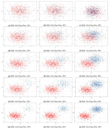
Figure 3.
Distribution of the artificial datasets in different configurations of imbalanced rate and overlapping. The red x represents the negative class, while the blue + represents the positive class.
These artificial datasets were created with 1000 instances, divided equally between two classes. The datasets have only two attributes to simplify the data visualization in 2D. The instances were generated using a random Gaussian distribution to fill the attributes’ values.
To create the overlapping effect, one of the classes had the mean of the distribution fixed, while the second class had its mean changed in the several values of distance from the first class. This difference was set from 0 to 5 with steps of 0.125.
To create an imbalanced dataset, the approach taken was that of removing instances from the target class. The instance number of the positive class was chosen to generate different levels of the imbalance dataset, starting in scenarios with a low level of imbalance and moving to more severe levels. The number of instance chosen can be checked in Table 1, in which they were placed to identify the imbalance, the information of the proportion of the positive class, and the number of the negative class.

Table 1.
Different levels of imbalance for the generation of artificial bases.
An example of the distributions is displayed in Figure 3. In the figure, 15 of the artificial datasets created are displayed in a 2D graph. As can be noticed, low values of the difference between the classes average create a large class overlapping; as this value is increased, the data increase their separability until the classes are completely separated.
To verify the behavior of the data outside a controlled environment, it was decided to test the methods on 12 datasets taken from the UCI repository [27]. These datasets are summarized in Table 2 and represent different data characteristics in relation to number of attributes, instances, and class balance.

Table 2.
Summary of the UCI tables used in this experiment.
The methods require two groups of hyperparameters, the threshold values, and a defined SOM. It is necessary to test the methods in the selected datasets to define the different values for these hyperparameters.
For the values of the thresholds ThresholdHigh and ThresholdLow, the value of the entropy threshold was experimented from 0.0 to 1.0, with steps of 5% in the difference between the classes. This is represented in Table 3 that shows the ratio between the classes inside the node and the respective entropy value. These entropy values were used as the different hyperparameters for our tests.

Table 3.
The different entropy values used in the experiment.
For the SOM hyperparameters, a hexagon grid of equal sides was used. The different lengths of the grid size were calculated as defined in Equations (5) and (6), with having the values of :
The next step was to compare the classification of the different datasets with the classification of the 1NN without pre-processing to compare improvements. For the validation, the training and test datasets were separated using the 10-fold cross validation methodology.
To measure the performance, it was decided to use the accuracy, F-Score, and G-Mean to validate the impact of the methods. Both the F-Score and G-Mean are commonly used for the measurement of imbalanced data [28]. This imbalance is presented in some of the UCI datasets. The F-Score measures the effectiveness of the classifier focused on the positive class, while the G-Mean indicates that equal importance is given to both classes [15]. To calculate these measures, the confusion matrix was used to determine the classification performance in terms of the positive and negative classes.
The complexity measures F1, F3, N2, and D3 presented in Section 2.3 were used for all the UCI and artificial datasets.
5. Results
In Table 4, Table 5, Table 6 and Table 7, the best values of accuracy, F-Score, and G-Mean obtained with the different approaches are summarized in terms of their means and standard deviations. These values represent the best value obtained with different values of threshold and the length of the grid size for each dataset. In Table 4, Table 5 and Table 6, some of the 41 artificial datasets were chosen to represent the data. The top classifier for a dataset is highlighted in bold.

Table 4.
Results for artificial dataset with 50% of positive class.

Table 5.
Results for artificial dataset with 25% of positive class.

Table 6.
Results for artificial dataset with 10% of positive class.

Table 7.
Results for the UCI datasets.
Analyzing the results of artificial dataset, for the case of accuracy, which can be seen in Table 4, Table 5 and Table 6, the method proposed (FIS) resulted in significantly greater gains in the bases with high overlap, especially when there was a greater imbalance. A possible explanation for this good performance in the cases of high imbalance could be that given that the parameters were optimized for accuracy, a considerable portion of the positive class has been removed by this method, which favors the negative class, which, being in the majority, increases the accuracy value. This effect decreases as the base becomes more balanced and the gains become smaller. However, the effect does exist, including for the balanced bases.
With regard to the overlap, the profit margins are higher in the bases that have more overlap, and they decrease as the level of overlap decreases to the point that we no longer have any gains with these methods. This is so because the classes are already sufficiently separated on these bases, creating conditions for the 1NN classifier without processing to have high performance.
To continue the analysis of the artificial bases, different graphs were generated with the best results of G-Mean after the variation of the parameters of ThresholdHigh and ThresholdLow and . These values were compared with the result of the 1NN classifier without pre-processing (baseline). To demonstrate the overlap, the value of the difference between the class means on the artificial base was placed on the x-axis, with values close to zero having high overlap and values more distant from zero having less overlap. The graphs were also divided according to their imbalance, choosing some fundamental values. In this way, it is possible to observe the impacts of overlap and imbalance at the same time and to make comparisons between the three methods that were generated and the 1NN without any alteration. B-FIS had results similar to those of H-FIS as shown in Table 4, Table 5 and Table 6. This fact makes the gain curves of the two methods overlap. Thus, it was decided to hide the B-FIS curve in these graphics for better visualization.
From the results in Figure 4, it can be seen that the H-FIS and L-FIS methods showed the greatest gain in an intermediate range of the overlap level—between approximately 1.0 and 3.0 difference of mean. By analyzing this imbalance, it can be seen that the methods have greater benefits for an intermediate range of imbalance between 15% and 30%. However, in situations with more severe imbalance, such as 5% and 10%, these methods had lower gains compared to 1NN classifier without processing.
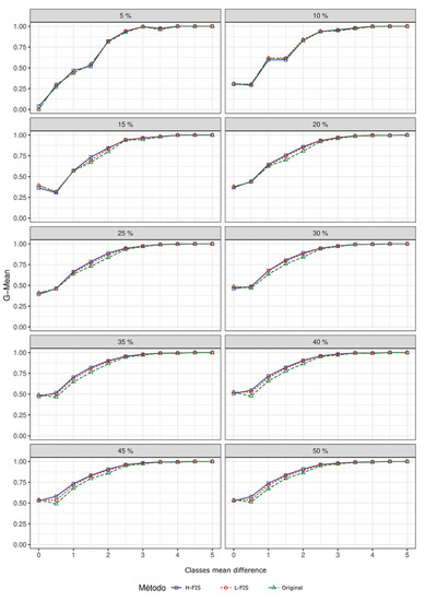
Figure 4.
Comparison of G-Mean values on artificial bases for the methods developed in this work and 1NN without pre-processing (baseline). The grouping was done by proportion of the positive class.
From the experiments summarized in Table 4, Table 6 and Table 7, all three methods showed an increase in accuracy, F-Score, and G-Mean when compared with the 1NN method on all datasets.
The use of the ThresholdHigh and ThresholdLow have the disadvantage of having an additional hyperparameter for the classifier. To simplify this fact, we examined the behavior of the thresholds in H-FIS and L-FIS and the effect on the G-Mean in the artificial dataset. This can be seen in Figure 5.
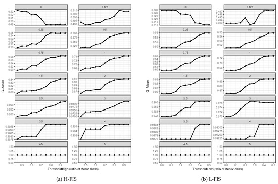
Figure 5.
Graphs that represent the effect of the H-FIS (a) and L-FIS (b) on G-Mean in the artificial datasets as we adjust the process to be more aggressive in the removal of points. The point to the left of the graph represents the initial point without pre-processing.
From the artificial datasets, the analyses of the threshold graphs indicate that the best results are in areas where the threshold is more aggressive, especially in areas with high class overlapping. The exception happens in the dataset with the largest overlapping where the difference between the classes averages is zero. It is also possible to verify that, when the classes are far apart, the method brought no benefits as there is no class overlapping.
For the next step, we calculated the complexity measures for the artificial datasets. The results for some of the datasets are summarized in Table 8.

Table 8.
Data complexity measures for the artificial datasets.
It is possible to use the data complexity values to evaluate the gain of the datasets compared to the complexity measures’ values. This way, it is possible to verify the behavior of the methods according to the increase of data complexity. In Figure 6, the results are shown for B-FIS. The behavior is similar for H-FIS and L-FIS.
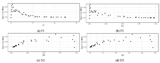
Figure 6.
Graphs that represent the gain of G-Mean using the B-FIS in the artificial datasets by the different complexity measures. In the case of F1 and F3, low values represent high class overlapping, while, for N2 and D3, low values represent low class overlapping.
As can be noticed in the graphs in Figure 6, this method has a range of class overlapping with the highest improvements, thus showing that this method is efficient in the original proposal of datasets with overlapping classes. However, in datasets with severe overlapping, indicated by very low values of F1, this method had only slight improvements in 1NN. The gain of the method reduces as the overlapping decreases, until the method no longer has a gain for the original 1NN.
To check if these conclusions are the same for other distributions of data, these procedures were repeated and compared for the UCI datasets. The data complexity measures that were calculated for the datasets are presented in Table 9 and Figure 7.

Table 9.
Data complexity measures for the real datasets.
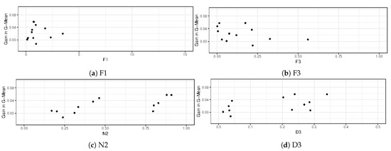
Figure 7.
Graphs that represent the gain of G-Mean using the B-FIS in the UCI datasets by the different complexity measures. In the case of F1 and F3, low values represent high class overlapping, while, for N2 and D3, low values represent low class overlapping.
As can be evaluated from the results in Figure 7, the gains of the methods cannot be explained by only the complexity measures. This behavior indicates that other characteristics of the data such as data distribution and data imbalance may impact the gains of B-FIS.
The analyses of the impact of the threshold values on the UCI datasets is shown in Figure 8. For L-FIS, there is a similar behavior of the artificial datasets, where the change in behavior happens in cases where a dataset suffers from a more severe overlapping. This is indicated by the low values of F1 and F3 in the cases of the datasets Haberman and Libra. However, in the case of H-FIS for the UCI datasets, there was no clear pattern even when compared with the data complexity measures.
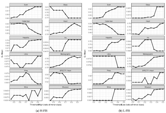
Figure 8.
Graphs that represent the effect of H-FIS (a) and L-FIS (b) on G-Mean in the UCI datasets as we adjust the process to be more aggressive in the removal of the points. The point to the left of the graph represents the initial point without pre-processing.
To better understand the effects of imbalance in the method, the effects of F1 were plotted against the gains of the F-Score dividing the classes’ imbalance ratio. The data can be found in Figure 9 and Figure 10.

Figure 9.
Graphs that represent the effect of the H-FIS (a) and L-FIS (b) on F-Score in the artificial datasets segregated by imbalance.

Figure 10.
Graphs that represent the effect of H-FIS (a) and L-FIS (b) on F-Score in the artificial datasets segregated by imbalance. The positive class ratio of that dataset is mentioned in parentheses.
From the results in Figure 9, it is possible to identify that higher levels of data imbalance caused higher gains with a certain range of low F1 values where this effect was enhanced.
Similarly, in the UCI datasets in Figure 10, the gains showed a similar pattern in intermediary ranges of imbalance and overlapping, especially in the case of L-FIS. The higher gains happened in datasets with more severe data imbalance.
To find the best size of SOM, the average maximum gain in F-Score was calculated for each value of with the help of Equation (5) for each dataset. The data were then ranked according to the F-Score value. An example of this process is summarized in Table 10 for the Ecoli dataset. The measure of the ranks in the datasets was calculated for each value of , and the average is summarized in Table 11. The best value is highlighted.

Table 10.
Ranked values of F-Score for for the Ecoli dataset.

Table 11.
Average rank of best F-Score for constant.
The best values, shown by the lowest average rank value, indicate that the best values for H-FIS and L-FIS occur in values close to the value zero; however, for B-FIS, the lowest values of are more effective.
It was decided to use the Wilcoxon signed-ranks test to validate whether the methods that were developed are statistically better than 1NN with no pre-processing. This test is appropriate for comparisons of classifiers over datasets [29].
The results for the UCI datasets are shown in Table 12. The results prove that the methods are statistically different with an , proving statistically that the methods enhance the classification of 1NN for the three different measures.

Table 12.
Calculated values of p using the Wilcoxon signed-ranks test for the UCI datasets.
Finally, a rough analysis carried out with the results available in the relevant literature is summarized in Table 13. As there is no structured dataset in the literature with separated training and test sets and a definition of the positive class in the dataset to investigate the algorithm performance in the overlap problem and imbalanced dataset, the comparison illustrated in this table is as shown in the papers cited. It may be noted that different algorithms show the best performance of G-Mean. The method proposed had good results which, in fact, were among the best results in the analyzed datasets.

Table 13.
Comparative results of G-Mean for the UCI datasets used in the literature.
6. Discussion
This work introduces three prototype selection methods that use SOMs and entropy to act as a filter for the selection of prototypes. Experiments using the methods were done both in a controlled environment to simulate class overlapping and with UCI datasets. These experiments showed that the methods improved the accuracy, F-Score, and G-mean values when compared with the common 1NN classifier in the different datasets.
The use of data complexity measures allowed quantifying the class overlapping in artificial datasets. These measures indicated that the methods had increased gains in overlapping scenarios in the artificial datasets according to the original proposal of the methods.
The methods have the disadvantage of requiring the setting of new hyperparameters ThresholdHigh and ThresholdLow for the classification process. To simplify this fact, we examined the behavior of the thresholds in H-FIS and L-FIS and the impact on method improvements. This can be seen in Figure 5 and Figure 8. L-FIS indicated a pattern of increased effectiveness with an increase in the value of ThresholdLow except for heavily overlapped datasets, which allows us to determine an ideal range based on an overlap measure, such as F1. H-FIS, however, did not show a clear pattern for ThresholdHigh.
The complexity measures allowed, by the analysis of F1, F3, and , indicating that these methods had good performances in databases with data overlapping. In addition, these methods showed increased gains in datasets with higher imbalance. However, the behavior of these methods could not be explained by only those measures, so other factors must affect the performance of the methods presented.
It would be interesting if further studies focus on trying some new situations, for instance, how these methods behave with noisy data and with different controlled environments involving imbalance and types of data distribution so that we can have a better comprehension of these methods. In addition, an extensive comparison with other algorithms can be done to have a better understanding of the benefits of the proposed methods.
Author Contributions
Conceptualization, M.R. and L.A.S.; methodology, M.R.; software, M.R.; validation, M.R. and L.A.S.; formal analysis, M.R. and L.A.S.; investigation, M.R.; resources, M.R.; data curation, M.R.; writing—original draft preparation, M.R.; writing—review and editing, M.R. and L.A.S.; supervision, L.A.S.; project administration, L.A.S.; funding acquisition, L.A.S. All authors have read and agreed to the published version of the manuscript.
Funding
This work was partially supported by CAPES (Coordenacao de Aperfeicoamento de Pessoal de Nivel Superior) with process number 88887.199212/2018-00 and Mackenzie (Universidade Presbiteriana Mackenzie).
Informed Consent Statement
Informed consent was obtained from all subjects involved in the study.
Data Availability Statement
The public datasets used in this work can be found in the UCI Machine Learning Repository https://archive.ics.uci.edu/ml/index.php (accessed on 9 June 2021).
Conflicts of Interest
The authors declare no conflict of interest.
References
- Vuttipittayamongkol, P.; Elyan, E. Improved overlap-based undersampling for imbalanced dataset classification with application to epilepsy and parkinson’s disease. Int. J. Neural Syst. 2020, 30, 2050043. [Google Scholar] [CrossRef]
- Elyan, E.; Moreno-Garcia, C.F.; Jayne, C. CDSMOTE: Class decomposition and synthetic minority class oversampling technique for imbalanced-data classification. Neural Comput. Appl. 2021, 33, 2839–2851. [Google Scholar] [CrossRef]
- Le, T.; Baik, S.W. A robust framework for self-care problem identification for children with disability. Symmetry 2019, 11, 89. [Google Scholar] [CrossRef] [Green Version]
- Yuan, B.W.; Luo, X.G.; Zhang, Z.L.; Yu, Y.; Huo, H.W.; Johannes, T.; Zou, X.D. A novel density-based adaptive k nearest neighbor method for dealing with overlapping problem in imbalanced datasets. Neural Comput. Appl. 2020, 33, 1–25. [Google Scholar] [CrossRef]
- Prati, R.C.; Batista, G.E.A.P.A.; Monard, M.C. Class Imbalances versus Class Overlapping: An Analysis of a Learning System Behavior. In Proceedings of the MICAI 2004: Advances in Artificial Intelligence, Mexico City, Mexico, 26–30 April 2004; Volume 2972, pp. 312–321. [Google Scholar] [CrossRef] [Green Version]
- Garcia, V.; Sanchez, J.; Mollineda, R. An empirical study of the behavior of classifiers on imbalanced and overlapped data sets. Prog. Pattern Recognit. Image Anal. Appl. Proc. 2007, 4756, 397–406. [Google Scholar] [CrossRef] [Green Version]
- Denil, M.; Trappenberg, T. Overlap versus imbalance. In Lecture Notes in Computer Science (Including Subseries Lecture Notes in Artificial Intelligence and Lecture Notes in Bioinformatics); Springer: Berlin/Heidelberg, Germany, 2010; Volume 6085 LNAI, pp. 220–231. [Google Scholar] [CrossRef] [Green Version]
- Wilson, D.R.; Martinez, T.R. Reduction Techniques for Instance-Based Learning Algorithms. Mach. Learn. 2000, 38, 257–286. [Google Scholar] [CrossRef]
- Cavalcanti, G.D.; Ren, T.I.; Pereira, C.L. ATISA: Adaptive Threshold-based Instance Selection Algorithm. Expert Syst. Appl. 2013, 40, 6894–6900. [Google Scholar] [CrossRef]
- Cavalcanti, G.D.; Soares, R.J. Ranking-based instance selection for pattern classification. Expert Syst. Appl. 2020, 150, 113269. [Google Scholar] [CrossRef]
- Rout, N.; Mishra, D.; Mallick, M.K. Handling imbalanced data: A survey. In International Proceedings on Advances in Soft Computing, Intelligent Systems and Applications; Springer: Berlin/Heidelberg, Germany, 2018; pp. 431–443. [Google Scholar]
- Le, T.; Lee, M.Y.; Park, J.R.; Baik, S.W. Oversampling techniques for bankruptcy prediction: Novel features from a transaction dataset. Symmetry 2018, 10, 79. [Google Scholar] [CrossRef] [Green Version]
- Cover, T.; Hart, P. Nearest neighbor pattern classification. IEEE Trans. Inf. Theory 1967, 13, 21–27. [Google Scholar] [CrossRef]
- García, S.; Derrac, J.; Cano, J.R.; Herrera, F. Prototype selection for nearest neighbor classification: Taxonomy and empirical study. IEEE Trans. Pattern Anal. Mach. Intell. 2012, 34, 417–435. [Google Scholar] [CrossRef]
- Branco, P.; Torgo, L.; Ribeiro, R.P. A Survey of Predictive Modeling on Imbalanced Domains. ACM Comput. Surv. 2016, 49, 1–50. [Google Scholar] [CrossRef]
- Kohonen, T. Essentials of the self-organizing map. Neural Netw. 2013, 37, 52–65. [Google Scholar] [CrossRef]
- Rubbo, M.; Silva, L.A. Prototype Selection Using Self-Organizing-Maps and Entropy for Overlapped Classes and Imbalanced Data. In Proceedings of the 2018 International Joint Conference on Neural Networks (IJCNN), Rio de Janeiro, Brazil, 8–13 July 2018; Volume 1, pp. 1–8. [Google Scholar] [CrossRef]
- Arabmakki, E.; Kantardzic, M. SOM-based partial labeling of imbalanced data stream. Neurocomputing 2017, 262, 120–133. [Google Scholar] [CrossRef]
- Douzas, G.; Bacao, F. Self-Organizing Map Oversampling (SOMO) for imbalanced data set learning. Expert Syst. Appl. 2017. [Google Scholar] [CrossRef]
- Moreira, L.J.; Silva, L.A. Prototype Generation Using Self-Organizing Maps for Informativeness-Based Classifier. Comput. Intell. Neurosci. 2017, 2017, 1–15. [Google Scholar] [CrossRef] [PubMed] [Green Version]
- Basu, M.; Ho, T.K. Data Complexity in Pattern Recognition; Springer: London, UK, 2006; p. 297. [Google Scholar] [CrossRef]
- Ho, T.K.; Basu, M. Complexity measures of supervised classification problems. IEEE Trans. Pattern Anal. Mach. Intell. 2002. [Google Scholar] [CrossRef] [Green Version]
- Sánchez, J.S.; Mollineda, R.A.; Sotoca, J.M. An analysis of how training data complexity affects the nearest neighbor classifiers. Pattern Anal. Appl. 2007, 10, 189–201. [Google Scholar] [CrossRef]
- Cano, J.R. Analysis of data complexity measures for classification. Expert Syst. Appl. 2013, 40, 4820–4831. [Google Scholar] [CrossRef]
- Morán-Fernández, L.; Bolón-Canedo, V.; Alonso-Betanzos, A. Can classification performance be predicted by complexity measures? A study using microarray data. Knowl. Inf. Syst. 2017, 51, 1067–1090. [Google Scholar] [CrossRef]
- Shannon, C.E. A Mathematical Theory of Communication. Bell Syst. Tech. J. 1948, 5, 3. [Google Scholar] [CrossRef] [Green Version]
- Dheeru, D.; Karra Taniskidou, E. UCI Machine Learning Repository. 2017. Available online: https://archive.ics.uci.edu/ml/index.php (accessed on 9 June 2021).
- He, H.; Garcia, E.A. Learning from imbalanced data. IEEE Trans. Knowl. Data Eng. 2009, 21, 1263–1284. [Google Scholar] [CrossRef]
- Demšar, J. Statistical Comparisons of Classifiers over Multiple Data Sets. J. Mach. Learn. Res. 2006, 7, 1–30. [Google Scholar]
- Fernandes, E.R.; de Carvalho, A.C. Evolutionary inversion of class distribution in overlapping areas for multi-class imbalanced learning. Inf. Sci. 2019, 494, 141–154. [Google Scholar] [CrossRef]
- Vuttipittayamongkol, P.; Elyan, E. Neighbourhood-based undersampling approach for handling imbalanced and overlapped data. Inf. Sci. 2020, 509, 47–70. [Google Scholar] [CrossRef]
- Yongqing, Z.; Min, Z.; Danling, Z.; Gang, M.; Daichuan, M. Improved SMOTEBagging and its application in imbalanced data classification. In IEEE Conference Anthology; IEEE: Piscataway, NJ, USA, 2013; pp. 1–5. [Google Scholar]
Publisher’s Note: MDPI stays neutral with regard to jurisdictional claims in published maps and institutional affiliations. |
© 2021 by the authors. Licensee MDPI, Basel, Switzerland. This article is an open access article distributed under the terms and conditions of the Creative Commons Attribution (CC BY) license (https://creativecommons.org/licenses/by/4.0/).