Experimental Evaluation of Heat Recovery Ventilators in Hot Climates

Abstract

This study investigates the thermal, economic, and environmental performance of heat recovery ventilators (HRVs) in hot climates, which has not been thoroughly investigated because standards and applications to date have focused primarily on cold climates. Experimental testing was conducted at airflow rates of 200–350 m³/h and outdoor air temperatures of 30–45 °C, representing typical summer conditions. HRV thermal performance was evaluated by measuring airflow rates and temperatures and then determining the heat transfer rates between the two air streams. Effectiveness increased by 3.9% when the supply inlet temperature increased from 30 to 45 °C, but decreased by 9.3% when airflow increased from 200 to 350 m³/h. The overall heat transfer coefficient remained nearly constant with increasing supply temperature but increased by approximately 37% as airflow increased. The highest recovery efficiency ratio (RER), defined as the ratio of supply air pre-cooling capacity to HRV power consumption, was 26.6 Btu/W.hr at 300 m³/h and 45 °C. Economic analysis based on the reduction in ventilation cooling load yielded payback periods ranging from 2.7 to 13.3 years. Annual CO₂ emission reductions ranged from 151 to 776 kg/year per HRV unit, demonstrating the environmental benefits of HRV systems in hot climates.

1. Introduction

Heat recovery ventilators (HRVs), also referred to as sensible recovery ventilators, are mechanical ventilation systems designed to improve indoor air quality and energy efficiency in residential, commercial, and industrial buildings. These units consist of two different airflow streams, one for bringing in fresh air from the outdoors (supply stream) and another for expelling stale air from occupied spaces (exhaust stream). As energy efficiency becomes a key consideration in building design, HRVs offer a valuable solution by pre-conditioning the incoming outdoor air, which in turn leads to energy savings [1].

In the winter, HRVs transfer thermal energy from the warm indoor air being exhausted to the colder outdoor air being brought in (i.e., supply air), thus pre-warming the fresh air before it enters the building. This winter application is the original historical focus of HRVs; however, in recent years, there has been significant interest in summer applications for hot climates, as in the present study. For this case, the process is reversed, and the warm incoming supply air loses thermal energy to the cooler indoor air being expelled, thus pre-conditioning the fresh outdoor air. In both summer and winter applications, the net effect of this pre-conditioning of outdoor air is to reduce the load on a building’s heating and cooling systems, especially where indoor air quality (IAQ) requirements dictate that fresh outdoor air be supplied to a building.

As noted, the HRV not only improves the operational energy efficiency of the installed HVAC system, but it also ensures a healthy and comfortable indoor environment by continuously exchanging stale indoor air with fresh outdoor air [2]. Inside the HRV core, where energy transfer occurs, the supply and exhaust air streams pass through multiple narrow, separate passages. This mechanical design allows for the transfer of thermal energy between the two air streams without any direct contact or mixing. As a result, while thermal energy is exchanged to either warm or cool the incoming fresh air (i.e., pre-conditioning), the contaminants from the exhaust stream, such as exhaled carbon dioxide, are kept separate and can thus be expelled from the building.

As noted, the study reported herein focuses on HRVs in hot weather conditions (i.e., summer months in hot climates), which is a research subject and application that has been largely ignored to date. This investigation gap between the two seasons (i.e., winter and summer) exists because HRVs were initially designed for cold weather use in northern regions during the winter, where well-insulated, tightly sealed homes mandated the use of HRVs to ensure energy efficiency and IAQ. As an aside, prior to implementing building standards in cold regions that emphasize decreasing envelope air leakage, it was generally accepted that for residential applications there was sufficient air leakage through joints, window seals, and around doors to maintain sufficient IAQ, which again changed as mandates for tighter homes were implemented.

2. Literature Review

Several studies have investigated HRVs operating in the summer cooling mode [3], primarily through performance simulations using software such as EnergyPlus and the Transient System Simulation Tool (TRNSYS). While some experimental studies have been conducted on a smaller scale, particularly for cold climate applications, most previous research has relied on simulations.

Guillén-Lambea et al. [4] conducted a TRNSYS simulation of Mediterranean area and found that the heat recovery ventilators significantly reduced energy demand. Lu et al. [5] evaluated the performance of a plastic film plate heat recovery ventilator operating in cross-flow mode. Their results showed that the effectiveness varied between 65% and 85% depending on the airflow rate. Wang et al. [6] presented a novel HRV. The proposed heat recovery unit achieved an average heat recovery effectiveness of 80% on a typical winter day and 74.7% during a typical transition season day, indicating better performance than conventional systems.

Jokisalo et al. [7] carried out a simulation study to investigate the performance of different mechanical ventilation systems in a residential building in Finland. It was found that a traditional exhaust ventilation system may use up to 67% more energy compared to a heat recovery system operating at 80% efficiency.

Yaïci et al. [8] presented a numerical analysis of HRVs using computational fluid dynamics, investigating the effect of varying different parameters under both winter (heating) and summer (cooling) operating conditions. The study found that increasing the flow velocity from 0.5 m/s to 2.5 m/s reduced the HRV effectiveness by approximately 34% for the co-current configuration and 20% for the counter-flow configuration. Also, it was found that increasing the supply temperature and relative humidity had no significant effect on the HRV effectiveness.

J. Fernández-Seara et al. [9] conducted an experimental parametric analysis on an HRV operating in cold weather conditions. The study found that increasing the airflow rate from 50 m³/h to 175 m³/h enhances the heat transfer rate by approximately 65%. However, effectiveness decreases from 94% to 78% over the same range.

Wen et al. [10] studied an HRV unit integrated with a radiant cooling panel system using EnergyPlus. Their analysis showed that the system decreased total energy use by up to 19.8%, and improved exergy efficiency from 16.1% to 21.1%.

Several researchers have proposed various strategies to reduce energy consumption in heat recovery ventilation (HRV) systems. These approaches generally focus on improving system performance through design enhancements [11,12,13], advanced control strategies [14,15], and the integration of HRV systems with other building energy systems [16,17,18]. The literature shows that most studies have focused on winter conditions, while summer cooling applications remain less investigated and are largely based on numerical simulations rather than experimental work. In this context, the present study experimentally investigates HRV performance under summer cooling conditions, addressing the limited availability of experimental data for hot weather operation and providing a clearer understanding of how HRV systems perform when sensible heat recovery is used to reduce cooling loads.

3. Experimental Overview

This section describes the test facility used in the current study, detailing the equipment and instrumentation. Additionally, experimental conditions and an analysis of the HRV unit’s performance are presented.

3.1. Experimental Setup

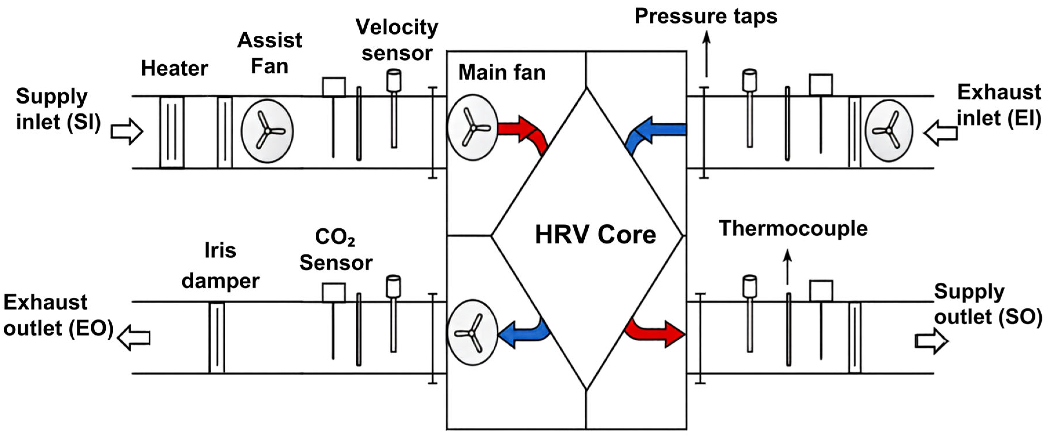
The test facility used in this study is equipped to perform experimental investigations and evaluations of both heat recovery ventilation (HRV) units and energy recovery ventilation (ERV) units, which are commonly referred to as H/ERV units, under realistic operating conditions. The HRV or ERV unit being tested and evaluated is centrally mounted in the testing facility, where it is connected to 152 mm diameter insulated supply and exhaust ducts. Outdoor fresh air and indoor return air entered the HRV through separate, insulated ducts connected to their respective inlets on opposite sides of the unit.

These ducts contain multiple sensors for measuring airflow rates, temperatures, pressures, CO₂ concentration, and RH levels in each of 4 separate flow streams entering and leaving, either on the supply or exhaust sides. Although the experimental facility is equipped with a multi-parameter sensor array, the present study focuses on the sensible thermal performance of the HRV. Accordingly, airflow velocity and temperature are the primary measurements used to determine heat transfer rates and thermal effectiveness. To ensure a uniform velocity profile and reduce flow disturbances before the air streams enter the heat exchanger core, flow straighteners are installed upstream within the HRV inlet ducts. In addition, a data acquisition system is configured for collecting and recording data while performance tests are being performed.

A laboratory air conditioning unit controls the temperature within the laboratory space to approximately 23 °C, which represents a simulated indoor temperature. To simulate a range of hot outdoor summer temperatures, a Tempco TDH01005 electric heater rated at 6 kW is placed in the inlet airflow stream of the supply duct. Iris dampers in the ducts regulate airflow by adjusting their opening size, while Systemair PrioAir 6 EC variable-speed inline fans at the supply and exhaust inlets assist the main fans within the HRV unit in achieving the desired airflow rates. Measurements are recorded only after the system achieves steady-state conditions to ensure repeatable and reliable heat exchanger performance.

Figure 1 is a schematic of the test facility layout, detailing the pathways of the supply and exhaust airflow streams, strategic instrument locations (e.g., airflow, pressure, temperature, CO₂ concentration, and RH levels) in the four connected ducts and the locations of major components, such as the HRV unit, fans, and the supply air heater.

3.2. Instrumentation

Hot-wire anemometers measure air velocity at four specific points within the ducting as illustrated in Figure 1. This velocity (m/s) is then multiplied by the duct’s cross-sectional area (m²) to determine the volumetric flow rate (m³/s). Thermocouples are used for temperature measurements (°C) of the air passing through all four duct segments. To ensure measurement accuracy and experimental reliability, all instrumentation was calibrated prior to testing. The velocity sensors were calibrated in the laboratory using a certified AMCA 210 airflow test chamber. The remaining sensors, including those used for temperature, pressure, CO₂ concentration, and relative humidity measurements, were calibrated by accredited laboratories certified to ISO/IEC 17025. Detailed specifications of all installed sensors, including sensing technology, measurement accuracy, and operating range, are summarized in

Table 1. Specifications of sensors.

Measured Parameter and Sensor	Manufacturer	Accuracy	Range
Velocity (Hot-wire anemometer)	E+E Elektronik (Engerwitzdorf, Austria)	±0.2 m/s plus 3% of measured value	0–20 m/s
Temperature (RTD)	OMEGA Engineering (Stamford, CT, USA)	±0.5 °C	−200 °C to 200 °C
RH (Capacitive polymer)	Dwyer Instruments (Michigan City, IN, USA)	±2%	10 to 100%
Pressure (Pressure Transducer)	Setra Systems (Boxborough, MA, USA)	±0.25%	0–746 Pa
CO2 (Non-dispersive infrared)	Vaisala (Vantaa, Finland)	±31 ppm	0–2000 ppm

.

3.3. Experimental Test Conditions

Table 2. Temperature and flow rate test conditions (i.e., independent variables).

Parameter	Value
Airflow rates	200–350 m3/h
Supply inlet temperatures	30–45 °C
Exhaust inlet temperature	23 °C

shows the operating test conditions for the three independent parameters. Efforts were made to ensure similar supply and exhaust flows, as tests were performed for a range of flow rates from 200 to 350 m³/h. The heater was equipped with a Watlow PM6C1CA PID controller to regulate the supply inlet temperature from 30 to 45 °C, which in turn represents the range of outdoor air temperature testing conditions. The exhaust inlet temperature, which simulates the indoor temperature, was fixed at 23 °C by the laboratory air conditioner. Because all intake air was drawn directly from the conditioned indoor laboratory space rather than raw outside air, variations in outdoor air quality, ambient particulate matter concentrations, and external Air Quality Index (AQI) were isolated and not used as experimental variables.

3.4. HRV Test Unit

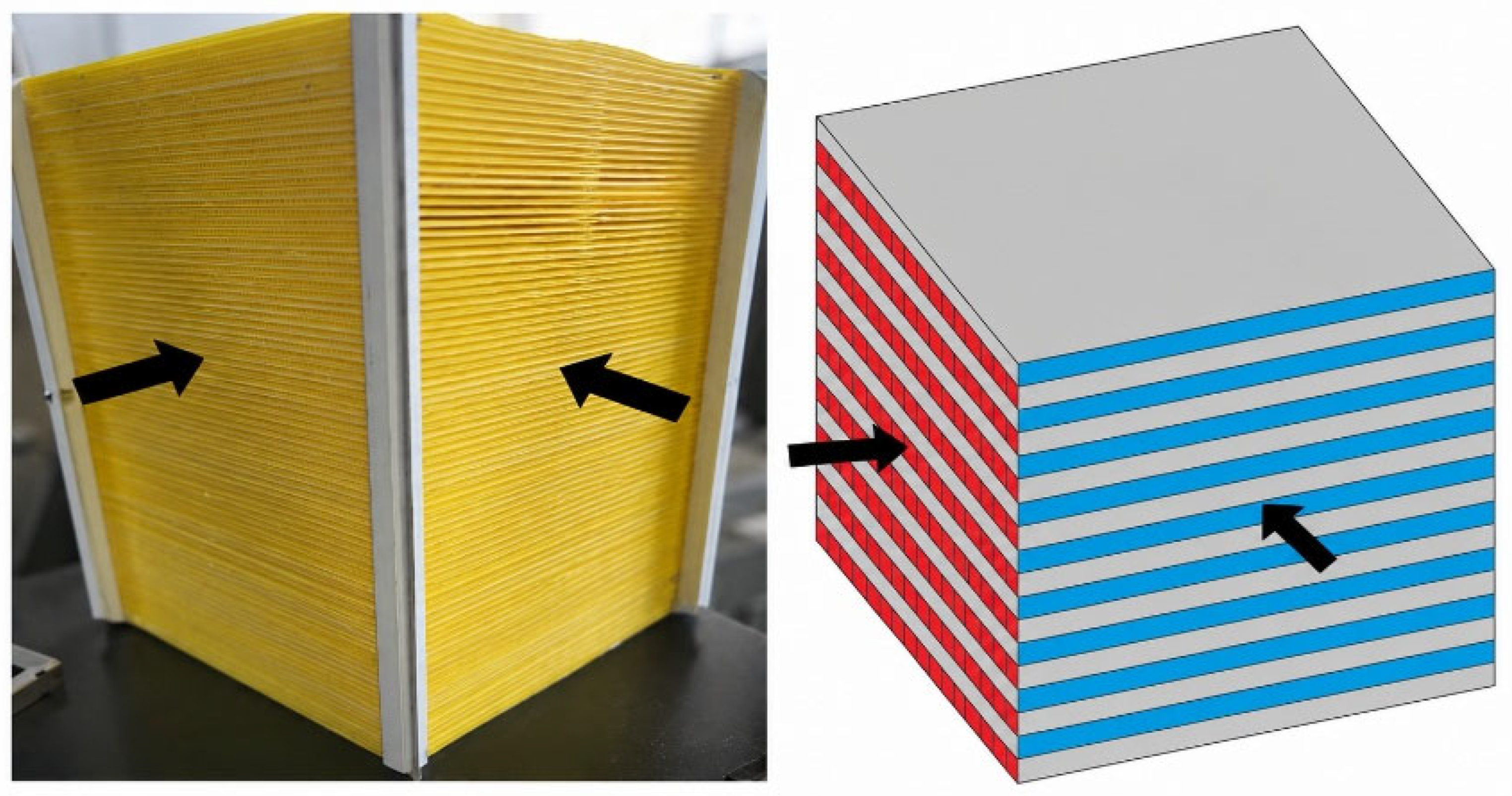
For the HRV unit investigated in this study, Figure 2 illustrates the 22.8 × 22.8 × 39.4 cm core, as constructed from polypropylene material. The unit was manufactured by Broan-NuTone (Canada). The heat exchanger core consists of alternating supply air and return airflow channels, featuring a channel height (plate spacing) of approximately 2.25 mm and a total of 168 flow channels, and a total heat exchange surface area of 4.6 m². Furthermore, this unit is a cross-flow, fixed plate-type structure designed to recover sensible heat only (unlike an ERV unit that recovers latent heat associated with water vapor transfer through a membrane). The core is enclosed in a pre-painted steel housing measuring 72.4 cm in length, 37.5 cm in height, and 39.4 cm in depth and is insulated with expanded polystyrene and sealed to minimize external influences.

To evaluate the performance of the commercially available HRV selected for this study, data collection was conducted under controlled conditions. Prior to testing, the facility and equipment underwent thorough inspection and maintenance; the unit’s washable particulate intake filters were cleaned, and the heat exchanger core surfaces were inspected and verified to be free of dust accumulation or physical obstructions. After setting up the test facility, the following steps were carried out to collect data and assess the HRV’s performance:

• The data acquisition (DAQ) system was initiated to collect real-time data from all installed sensors.
• The fans were adjusted to balance the supply and exhaust airflows at the target flow rate of 200–350 m³/h, while the PID-controlled duct heater was set to the target supply air temperature of 30–45 °C.
• The system was operated continuously until thermal and fluid steady-state conditions were achieved, which typically required more than 1 h. During this conditioning period, all measured parameters, including temperature, airflow rate, pressure, and relative humidity, were continuously monitored. Once the operating conditions stabilized, the system was maintained for an additional 10 min verification period. Steady-state conditions were confirmed when temperature fluctuations remained within ±0.2 °C and airflow rate fluctuations remained within ±1.5%.
• Following confirmation of steady-state conditions, data were continuously recorded for 30 min at each test condition.
• Each test condition was repeated five times, with the same conditioning and measurement procedure applied to each run. The time-averaged results from the repeated runs were then used for the subsequent analysis and reporting.

3.5. Performance Indices

The heat transfer rate ($\dot{Q}$) to or from the airflow on each side can be calculated from the conservation of energy applied to each air stream with major assumptions being steady state and zero heat transfer to or from the surroundings.

After applying the above assumptions to the general energy equation, the resulting heat transfer rate ($\dot{Q}$) formula for either the supply or exhaust side air, as a function of the air temperature change (∆T), is

$$\dot{Q}=\dot{m} C_p ∆T$$

(1)

where $\dot{m}$ is mass flow rate and C_p is the specific heat capacity for air. The mass flow rate can be found by multiplying the air volumetric flow rate by air density.

In addition to heat transfer rate, another important HRV performance factor is the experimental HRV effectiveness ($\epsilon$), which is defined as the ratio of actual heat transfer to the maximum possible heat transfer, with the defining equation as follows [19]:

$$\epsilon ={\displaystyle \frac{{\dot{C}}_{so} \left(T_{si}-T_{so}\right)}{{\dot{C}}_{min} \left(T_{si}-T_{ei}\right)}}$$

(2)

where T is the temperature in each flow stream and the subscripts are o-outlet, i-inlet, s-supply, and e-exhaust. In addition, ${\dot{C}}_{so}$ represents the capacity rate ($\dot{C}=\dot{m}{C}_p$) at the supply outlet, and ${\dot{C}}_{min}$ denotes the minimum capacity rate, either on the supply or exhaust side, when the two sides are compared. In the case of HRV testing and data analysis, the flow rates on both sides are assumed to be the same so that in principle the above equation can be simplified by cancelling the two capacity rates.

Cancelling out the capacity rates in Equation (2) results in the effectiveness being equal to the measured temperature change for either of the fluids divided by the maximum possible temperature difference, which is the supply inlet temperature (T_si) minus the exhaust inlet temperature (T_ei) as follows:

$$\epsilon ={\displaystyle \frac{ \left(T_{si}-T_{so}\right)}{ \left(T_{si}-T_{ei}\right)}} ={\displaystyle \frac{ \left(T_{eo}-T_{ei}\right)}{ \left(T_{si}-T_{ei}\right)}}$$

(3)

To evaluate the Second Law performance of the HRV system, the exergy efficiency (${\eta }_{ex}$) is defined as the ratio of the recovered thermal exergy to the total exergy input required for operation, including the available thermal exergy and the electrical energy consumed by the fans:

$${\eta }_{ex}={\displaystyle \frac{{\dot{EX}}_{recovered}}{{\dot{EX}}_{expended}+ {\dot{P}}_{fans}}}$$

(4)

The thermal exergy rate associated with each air stream is calculated as

$$\dot{EX}=\dot{m}{C}_p\left[\left(T-T_0\right)-T_0\ln \left({\displaystyle \frac{T}{T_0}}\right)\right]$$

where $\dot{m}$ is the air mass flow rate, $C_p$ is the specific heat capacity of air, $T$ represents the temperature of each air stream, and $T_0$ is the ambient reference environment temperature.

A fourth important HRV parameter is the overall heat transfer coefficient, the U-value. The rate of thermal energy transfer between the two air streams can be calculated as follows:

$$\dot{Q}=UA LMTD$$

(5)

where A is the HX area and LMTD is the log mean temperature difference, which is defined as

$$LMTD={\displaystyle \frac{∆T_1-∆T_2}{\ln \left(\frac{∆T_1}{∆T_2}\right)}}$$

(6)

with ∆T₁ and ∆T₂ being the supply-to-exhaust side temperature difference at each end of the HRV.

Conversely, the above equation can be rearranged to solve for the U-value of the HRV if the total heat exchange area, the heat transfer rate, and the LMTD are known from flow rate and temperature measurements, as follows:

$$U={\displaystyle \frac{\dot{Q}}{A LMTD}}$$

(7)

The recovery efficiency ratio (RER) is a metric used to evaluate the performance of recovery ventilators. It is similar to the energy efficiency ratio (EER) used for air conditioning systems where EER is the ratio of cooling capacity (Btu/hr) and power consumed by the prime movers, such as the compressor and fans (kW). In one sense, EER is the ratio of useful energy transfer rate (Btu/hr) and cost of operation (kW) knowing that each kW-hr of energy has a cost associated with it. Similarly, RER represents the ratio of energy rate recovered (Btu/hr) and the power consumed (kW), which in this study refers to the HRV fans, with the final results being

$$RER={\displaystyle \frac{{\dot{Q}}_{Recovered}}{{\dot{P}}_{fans}}}$$

(8)

The energy rate recovered is the heat transfer rate from the supply side that is transferred to the exhaust side, while fan power is a measured parameter.

3.6. Uncertainty Analysis

An uncertainty analysis was conducted to evaluate the propagation of experimental errors in the primary thermal performance parameters: the heat transfer rate ($\dot{\mathrm{Q}}$) and sensible effectiveness (ϵ). Using the root-sum-square propagation method for uncorrelated independent variables (Kline and McClintock method):

$$U_R=\sqrt{{\displaystyle \sum _{i=1}^n}{\left({\displaystyle \frac{\partial R}{\partial x_i}}{U}_{x_i}\right)}^2}$$

(9)

where $U_{x_i}$ represents the absolute uncertainty of each measured variable obtained from instrument specifications, and $U_R$ is the propagated uncertainty of parameter $R$.

For the heat transfer rate ($\dot{Q}$), the propagated uncertainty depends on individual errors in airflow velocity, temperature measurements, and air properties. Across the evaluated operating conditions, the uncertainty of $\dot{Q}$ ranged from $\pm 30 \mathrm{W}$ to $\pm 105 \mathrm{W}$. For sensible effectiveness ($ϵ$), which depends on temperature differences across the exchanger streams, the calculated uncertainty ranged from $\pm 0.8\%$ to $\pm 2.6\%$ across the full test range.

4. Results and Discussion

4.1. Thermal Performance Results

This section presents the thermal performance of an HRV unit for the range of airflow rates and supply inlet temperatures, which were presented earlier in the test condition matrix.

4.1.1. Heat Transfer Rate

The first step in determining and analyzing the HRV thermal performance is to investigate the impact of volumetric airflow rate and supply inlet temperature on heat transfer rates. As previously noted, the HRV is designed and assumed to recover only sensible heat. While condensation can occur in practice if the supply air stream temperature falls below its dew point, this condition was avoided in the current tests. Specifically, a heater was used to simulate elevated indoor temperatures by heating the supply air drawn from the laboratory, which consequently reduced its relative humidity and effectively eliminated the possibility of condensation during testing, especially since the laboratory air temperature is the same as the exhaust air inlet temperature.

Table 3. Heat transfer rate at various flow rates for T_si = 35 °C.

Volumetric Airflow Rate [m3/h]	Heat Transfer Rate [W]		Standard Deviation [W]		Difference [W]	Percentage Difference [%]
	Supply	Exhaust	Supply	Exhaust
200	480	494	10	19	14	2.9
250	598	604	16	22	6	1
300	697	713	10	13	16	2.3
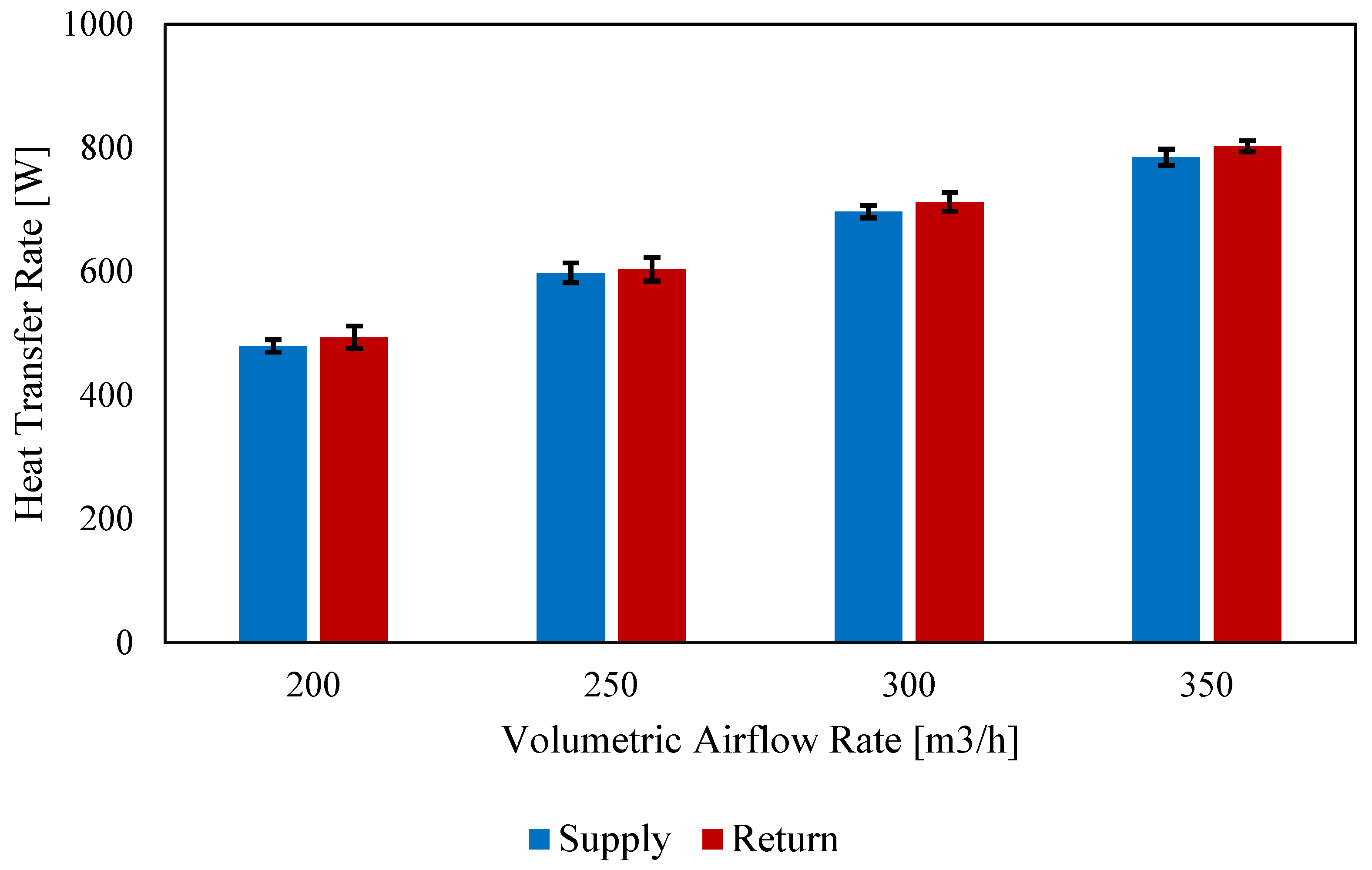
350	785	803	13	21	18	2.3

and Figure 3 show that as the airflow rate increases the HRV heat transfer rate also increases. For example, it can be seen that as the flow rate increases from 200 to 350 m³/h, the supply-side heat transfer rate increases by 64% from 480 W to 785 W. This increase in heat transfer rate is the result of both an enhanced convective heat transfer coefficient and a larger temperature difference between the hot and cold side air over the HX length as flow rate increases. To verify the reliability and accuracy of the experimental data, the overall energy balance was evaluated by calculating the heat balance deviation between the supply and exhaust air streams. Across the tested airflow rates in Table 3, the heat transfer rate differences remained small, ranging between 1.0% and 2.9% with an average heat balance deviation of 2.1%. This minor variation is well within acceptable engineering limits and can be attributed to minimal ambient heat losses through the insulated HRV housing, as well as the inherent measurement uncertainty of the flow sensors. Table 3 also shows the standard deviations of heat transfer rates. One can conclude that the supply and exhaust side heat transfer rate difference are in most cases similar in magnitude to the standard deviations on each of the plots and curves, indicating that the supply and exhaust side heat transfer rates are in fact equivalent.

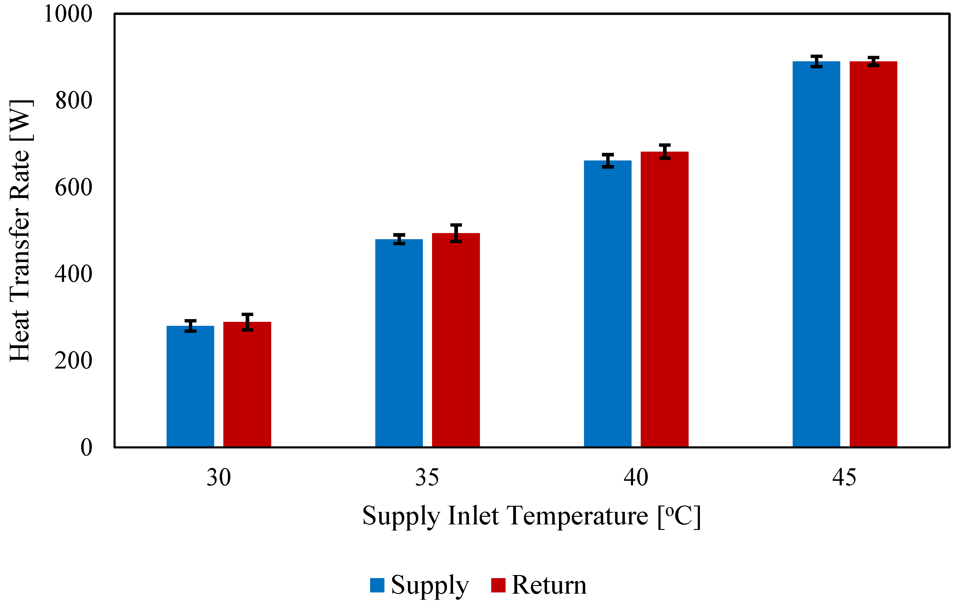
The heat transfer rates of the HRV unit at 200 m³/h for various supply inlet temperatures are tabulated in

Table 4. Heat transfer rate at various supply inlet temperatures for V = 200 m³/h.

Supply Inlet Temperature [°C]	Heat Transfer Rate [W]		Standard Deviation [W]		Difference [W]	Percentage Difference [%]
	Supply	Exhaust	Supply	Exhaust
30	280	289	12	18	9	3.2
35	480	494	10	19	14	2.9
40	661	682	14	15	21	3.1
45	890	890	12	9	0	0

and plotted in Figure 4. It can be observed that as the supply inlet temperature is increased from 30 to 45 °C, then the heat transfer rate on the supply side increases from 280 W to 890 W. This increase is primarily due to the larger temperature difference between the supply air and the exhaust air, which in turn enhances the driver for heat exchange in the HRV. To ensure the reliability of these data across varying thermal conditions, the heat balance deviation between the supply and exhaust sides was evaluated. The differences remained small, ranging from 0.0% to 3.2% with an average deviation of 2.3% for this temperature range. These minor variations are primarily attributed to minimal ambient heat losses through the insulated HRV housing and the inherent measurement uncertainty of the sensors. Since the differences in heat transfer rates between the supply and exhaust sides are often similar in magnitude to their respective standard deviations, it can be concluded that the bars in the chart (with error bars representing standard deviations) show no significant difference.

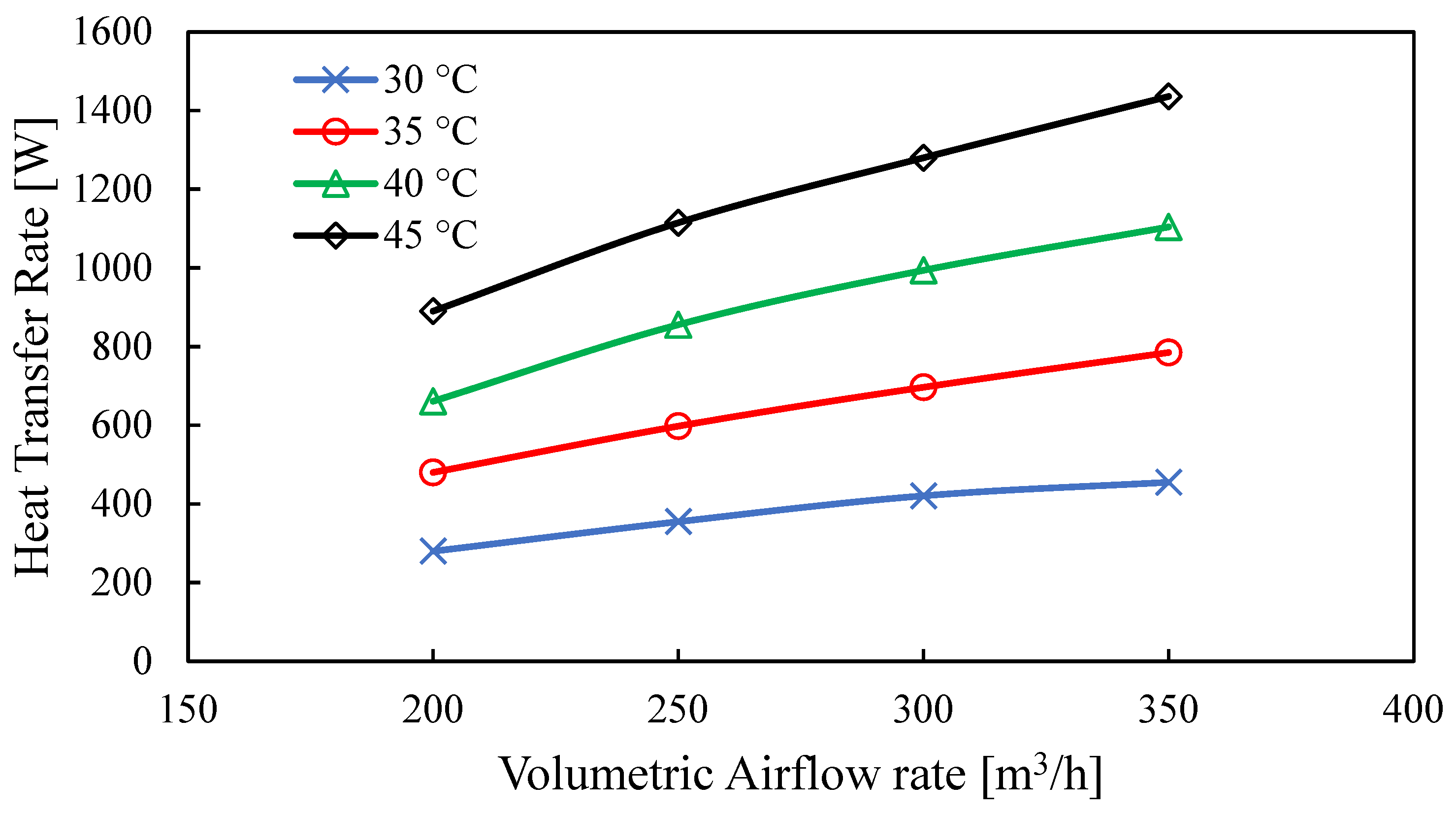
The full impact of volumetric flow rates and supply inlet temperatures (i.e., outdoor temperature) on the heat transfer rates of the HRV unit are tabulated in

Table 5. HRV heat transfer at various flow rates and supply inlet air temperatures.

Volumetric Airflow Rate [m3/h]	Heat Transfer Rate [W]
	Tsi = 30 °C	Tsi = 35 °C	Tsi = 40 °C	Tsi = 45 °C
200	280	480	661	890
250	355	598	856	1115
300	421	697	994	1280
350	455	785	1104	1436

and plotted in Figure 5. It can be observed that as the flow rate increases from 200 to 350 m³/h, then the heat transfer rate increases. For example, over this flow range with a fixed supply air of 30 °C and 45 °C, the heat transfer rate increases by 63% from 280 to 455 W and by 61% from 890 to 1436 W, respectively.

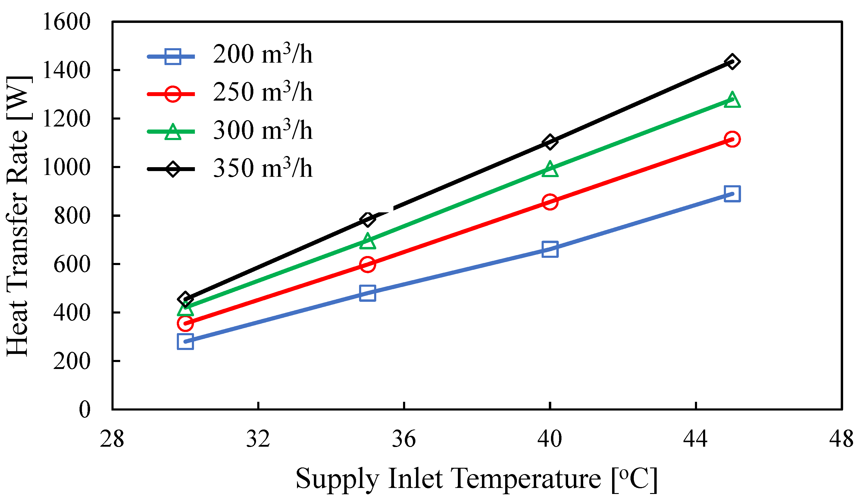
The effect of increasing supply temperature can also be observed in Figure 5; however, these effects are better observed in a plot of heat transfer rate versus supply inlet temperature for a range of flow rates as in Figure 6. Specifically, it can be observed in Figure 6 that as the supply inlet temperature increases, then the heat transfer rate increases. For instance, at a flow rate of 350 m³/h, as the supply temperature rises from 30 °C to 45 °C, the heat transfer rate increases by 216% from 455 to 1436 W, while at a lower flow rate of 200 m³/h, the heat transfer rate increases by 218% from 280 to 890 W. The reason that the heat transfer rate increases with supply inlet temperature is that the driving temperature difference for heat transfer increases as the supply inlet temperature increases.

It should be noted that while airflow rate and inlet temperature were the primary parameters investigated, the heat transfer rate is also influenced by the heat exchanger design. The present study was conducted using a commercially available polypropylene cross-flow fixed plate HRV operated under balanced supply and exhaust airflow conditions. Other design parameters, including core material, flow arrangement, heat transfer surface area, and airflow balance, also affect the overall heat transfer coefficient and consequently the heat transfer rate. Therefore, the heat transfer rate values reported in this study are representative of the tested HRV configuration, whereas the observed trends with airflow rate and inlet temperature are expected to be applicable to similar sensible heat recovery ventilators.

4.1.2. Effectiveness and Exergy Efficiency

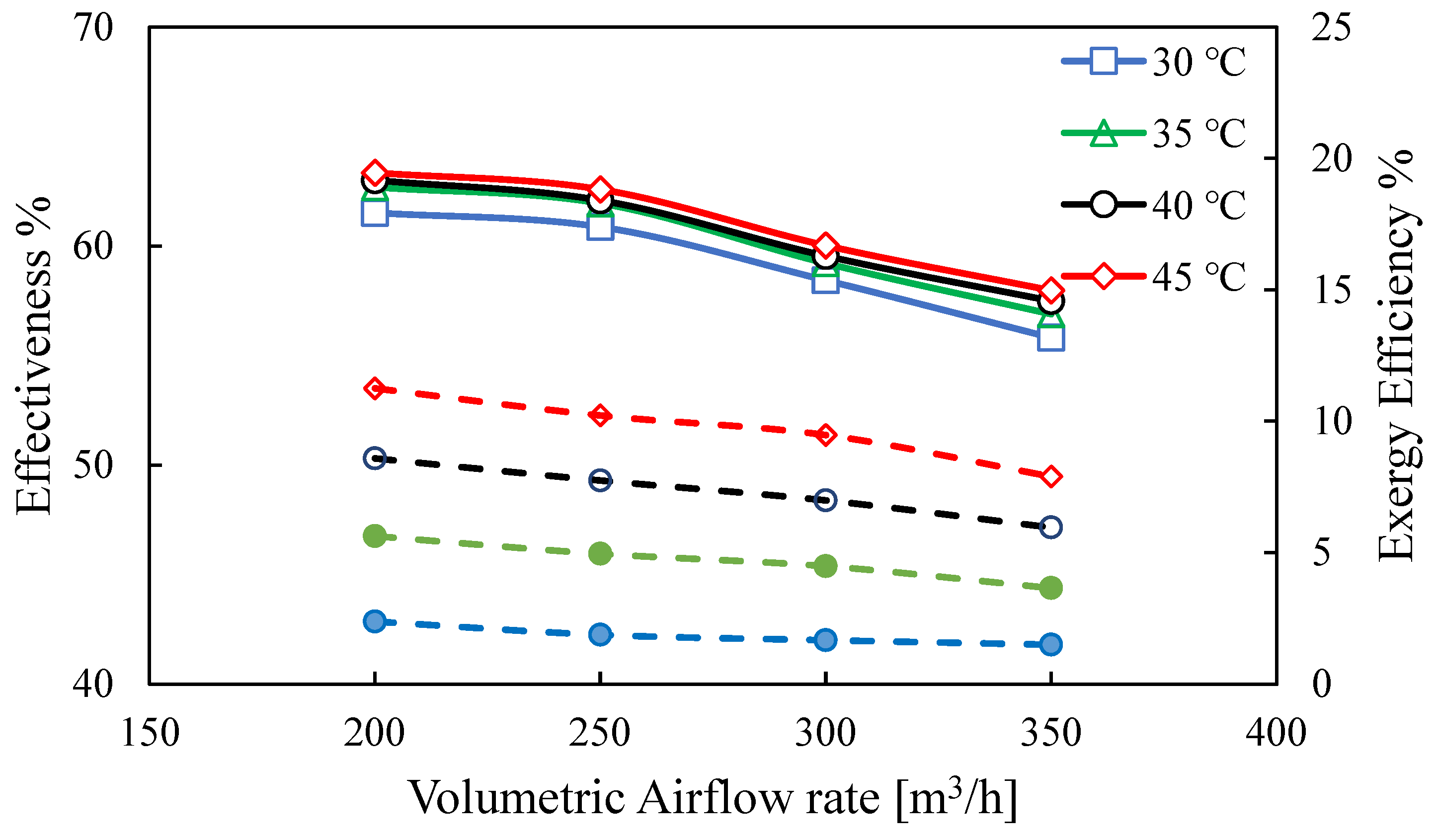
The effectiveness of a heat recovery ventilator (HRV) is a critical indicator of its thermal performance. In the case of cooling in hot climates, which is the focus of the study reported herein, a higher effectiveness means the system can pre-cool more of the hot supply-side air, so that it discharges into the building space at a lower temperature than it otherwise would, and as a result, the need for supplemental cooling is reduced, which is an energy saving. Effectiveness can also be understood by realizing that it is the fraction of the maximum possible heat transfer rate that is transferred from the supply side to the exhaust side. The impact of volumetric flow rate and supply inlet temperature on the effectiveness and exergy efficiency of the HRV unit are tabulated in

Table 6. HRV effectiveness at various flow rates and supply inlet air temperatures.

Volumetric Airflow Rate [m3/h]	Performance Metric	Tsi = 30 °C	Tsi = 35 °C	Tsi = 40 °C	Tsi = 45 °C
200	ε [%]	61.5	62.7	63	63.4
	ⴄex [%]	2.4	5.6	8.6	11.3
250	ε [%]	60.9	62.0	62.1	62.6
	ⴄex [%]	1.9	5	7.7	10.2
300	ε [%]	58.4	59.2	59.6	60
	ⴄex [%]	1.7	4.5	7	9.5
350	ε [%]	55.8	56.9	57.5	58.0
	ⴄex [%]	1.5	3.7	6	7.9

, and effectiveness alongside exergy efficiency versus airflow rate is plotted in Figure 7. It can be observed that the effectiveness decreases as the volumetric airflow rate increases. For example, at 30 °C the effectiveness decreases from 61.5% to 55.8%, and at 45 °C it decreases from 63.4% to 58.0% as the volumetric flow increases from 200 to 350 m³/h. Similarly, the exergy efficiency decreases as the flow rate increases. For example, at 45 °C it decreases from 11.3% to 7.9% as the volumetric flow increases from 200 to 350 m³/h. One possible explanation is that a reduced residence time results as the flow rate of air increases, meaning the air spends less time in contact with the heat exchanger surfaces, leading to a decrease in HRV effectiveness. With that said, it should also be observed that even when the flow rate doubles, the reduction in effectiveness is less than 10%, meaning the airflow rate does not significantly affect HRV effectiveness.

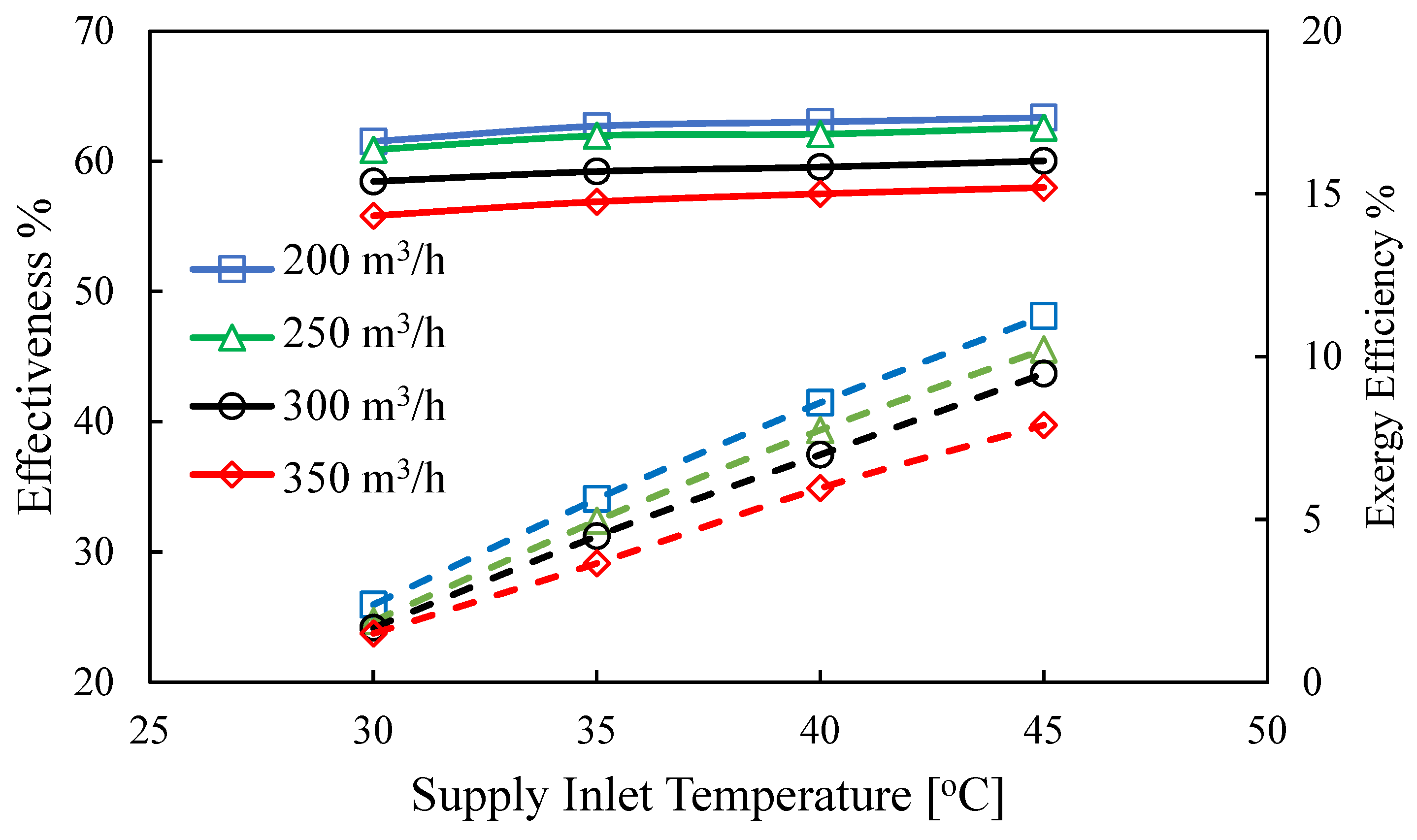
The effect of the supply inlet temperature on effectiveness and exergy efficiency is better understood by plotting effectiveness versus temperature for a range of flow rates as shown in Figure 8. It can be observed in Figure 8 that as the supply inlet temperature increases, effectiveness also increases. For example, as the temperature increases from 30 °C to 45 °C at a volumetric flow rate of 200 m³/h, the effectiveness increases from 61.5% to 63.4%, which is a 3.1% change in effectiveness, indicating that effectiveness is only a weak function of supply inlet temperature, which is similar to flow rate as was shown previously. Conversely, the overall exergy efficiency is more sensitive to the supply inlet temperature, increasing from 1.5% at 30 °C to 11.3% at 45 °C. Unlike sensible effectiveness, which only measures the amount of heat recovered, the overall exergy efficiency considers both the quality of the recovered thermal energy and the electrical energy consumed by the HRV fans. As the supply inlet temperature increases relative to the ambient reference temperature ($T_0$), the recovered heat contains more useful energy, leading to a higher exergy efficiency. In contrast, increasing the airflow rate leads to increased fan power consumption while reducing the time air remains inside the heat exchanger, causing the overall exergy efficiency to decrease. Overall, comparing these two metrics highlights a clear difference between heat quantity and energy quality. While effectiveness measures only the proportion of heat transferred within the recovery core, overall exergy efficiency assesses the quality of that recovered heat relative to the reference environment ($T_0$), while simultaneously accounting for the electrical power consumed by the fans (${\dot{P}}_{\mathrm{fans}}$). As a result, the two metrics can react quite differently under changing conditions—exergy efficiency is more sensitive, exhibiting much faster rates of change and yielding significantly different numerical values compared to the relatively stable thermal effectiveness.

The thermal effectiveness values obtained in this study ranged from 55.8% to 63.4%. Reported effectiveness values in published studies vary widely [20], as differences in core geometry, plate configuration, flow arrangement, heat and mass transfer materials, and operating conditions significantly influence performance. Higher effectiveness values reported in some studies may be associated with lower airflow rates or increased heat transfer capacity, such as through larger heat transfer areas or enhanced heat exchanger designs. Therefore, direct performance comparisons among different HRV systems should consider the specific design characteristics and operating conditions of each system.

4.1.3. U-Value

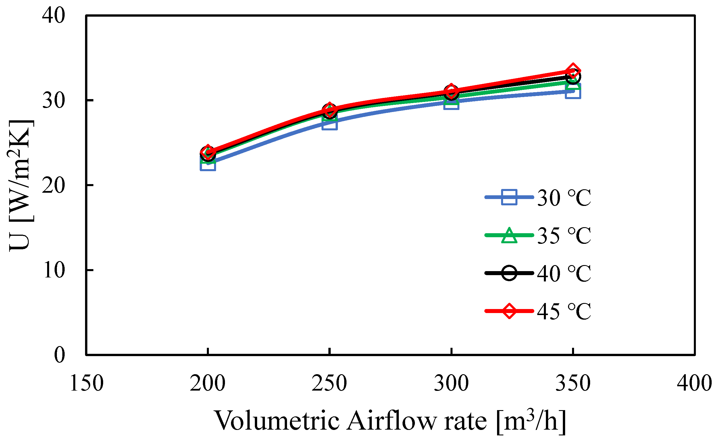
The overall heat transfer coefficient (U) is a measure of the HX’s ability to transfer heat for a given driving temperature difference, as presented earlier.

Table 7. U-value of HRV at various flow rates and supply inlet temperatures.

Volumetric Airflow Rate [m3/h]	U [W/m2K]
	Tsi = 30 °C	Tsi = 35 °C	Tsi = 40 °C	Tsi = 45 °C
200	22.6	23.5	23.7	23.9
250	27.4	28.5	28.7	28.9
300	29.8	30.4	30.9	31.1
350	31.1	32.2	32.8	33.5

along with Figure 9 shows the impact of flow rate on the U-value. It can be observed that as the flow rate increases from 200 to 350 m³/h, then the U-value increases. For example, as the flow rate increases at a supply temperature of 35 °C, the U-value increases from 23.5 to 32.2 W/m²K, which is about a 37% increase. Higher flow rates and internal velocities increase mixing and turbulence within the HRV’s two flow streams, which in turn leads to larger values of internal convection heat transfer coefficients, resulting in U-value increases as can be seen in Figure 8.

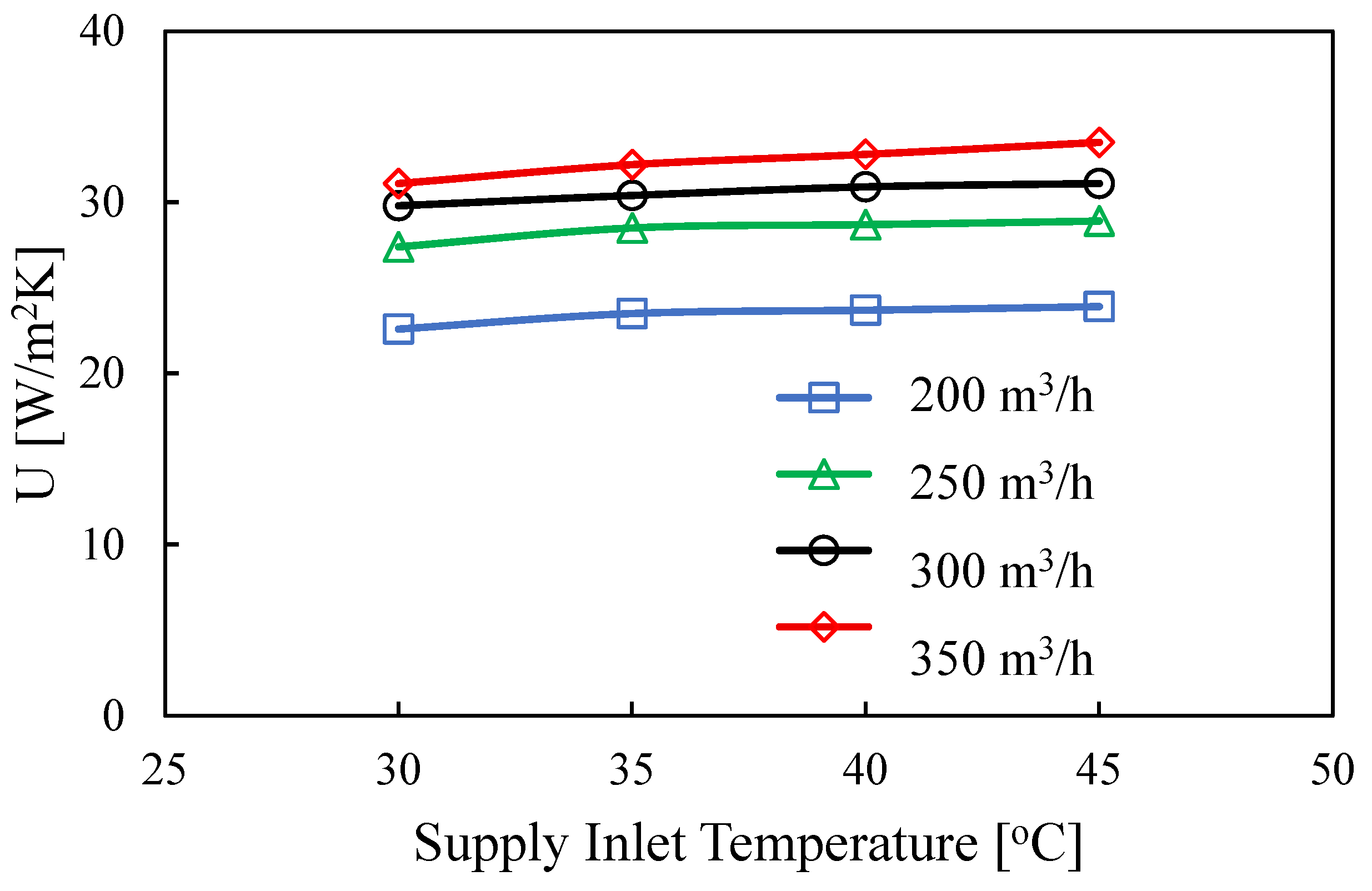
The impact of the supply inlet temperatures on U-values for a range of volumetric flow rates is plotted in Figure 10. The U-value remains almost constant for each airflow rate, with only a slight increase observed as the supply inlet temperature rises from 30 to 45 °C. For example, at 200 m³/h, U changes from 22.6 W/m²K to 23.9 W/m²K, and at 350 m³/h, from 31.1 W/m²K to 33.5 W/m²K.

4.1.4. Recovery Efficiency Ratio

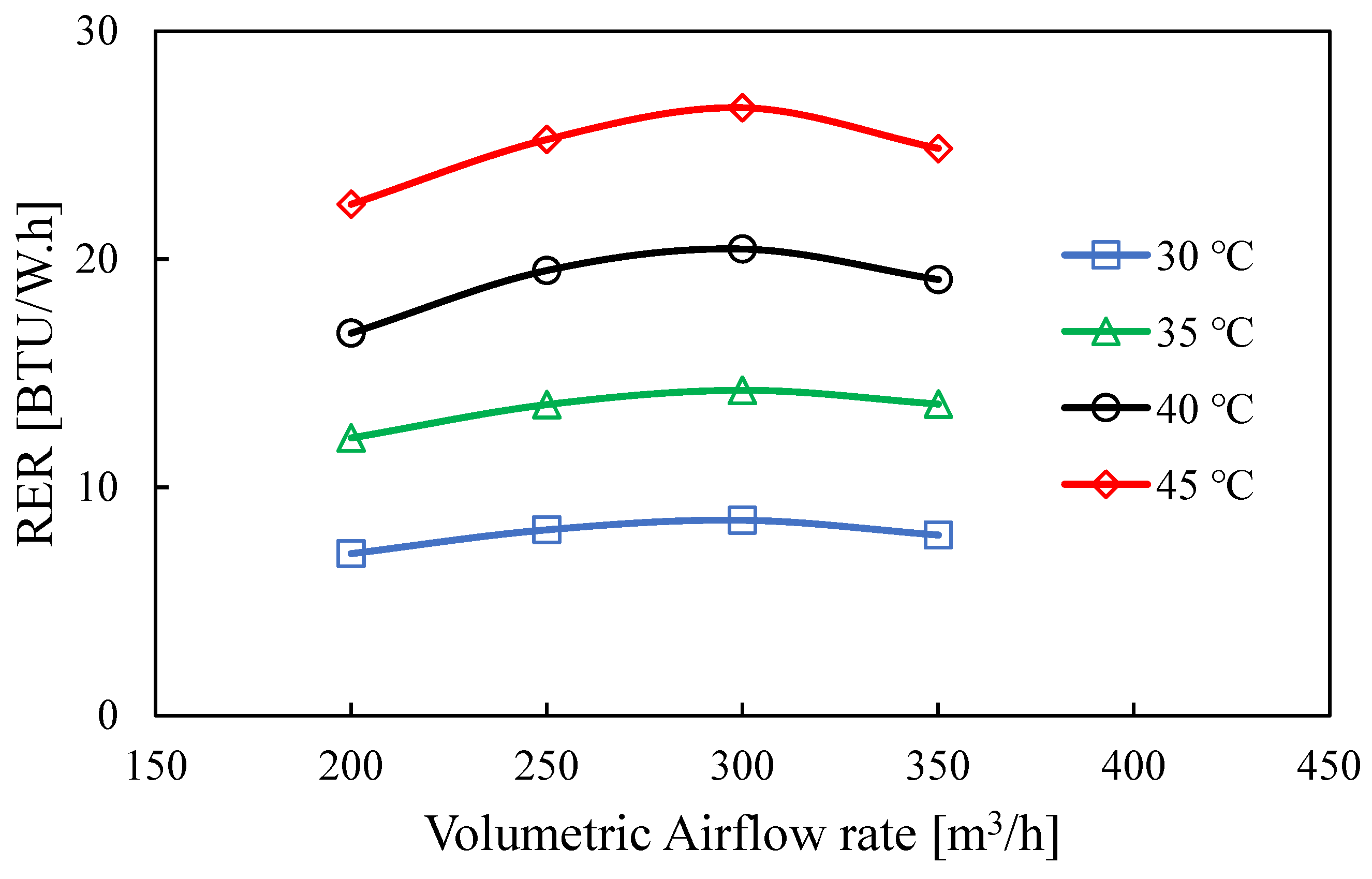
The recovery efficiency ratio (RER) is defined as the ratio of supply air pre-cooling to the HRV unit’s power consumption required to achieve this level of pre-cooling, as shown in

Table 8. RER value at various flow rates and different supply inlet temperatures.

Volumetric Airflow Rate [m3/h]	RER [Btu/W.h]
	Tsi = 30 °C	Tsi = 35 °C	Tsi = 40 °C	Tsi = 45 °C
200	7.1	12.2	16.8	22.4
250	8.1	13.6	19.5	25.2
300	8.6	14.3	20.4	26.6
350	7.9	13.7	19.1	24.9

and plotted in Figure 11. RER varies with airflow rates and supply inlet temperature. For example, it can be observed that as the volumetric airflow rate increases from 200 to 300 m³/h at 35 °C, the RER rises from 12.2 to a peak of 14.3 Btu/W·h. However, as the airflow rate increases further to 350 m³/h, the RER decreases slightly to 13.7 Btu/W·h. This behavior occurs because higher airflow rates lead to greater pressure losses, resulting in a non-linear increase in power consumption. This peak behavior is most evident at higher inlet temperatures, particularly at 45 °C, where the RER values are significantly higher compared to values at lower temperatures. The effect of air temperature is explored below where RER is plotted versus supply inlet temperature.

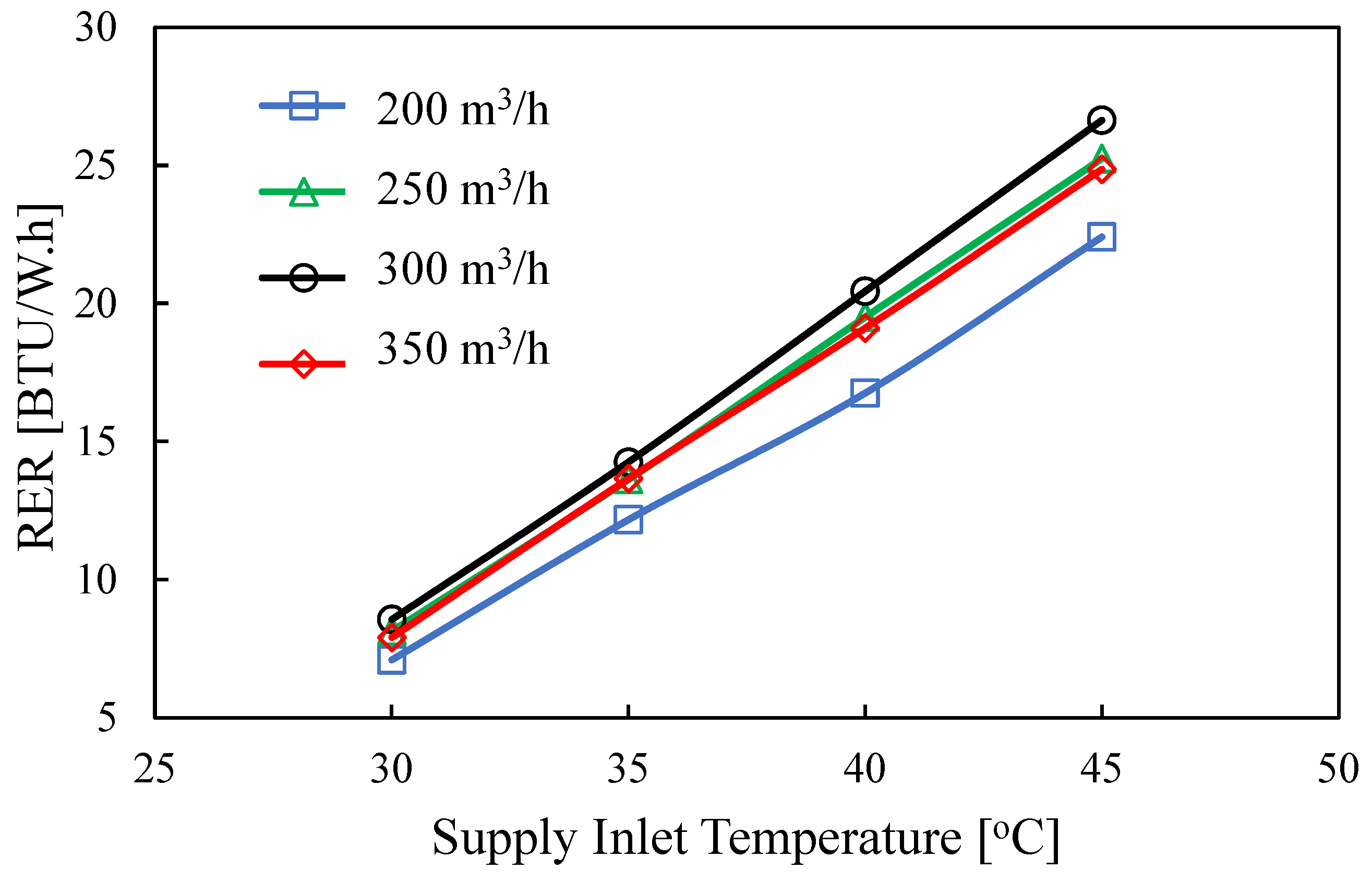
As noted above, RER versus supply inlet temperature or a range of flow rates is plotted in Figure 12, where it can be observed that as the supply inlet temperature increases, the RER increases. For example, at a flow rate of 200 m³/h, as supply temperature increases from 30 to 45 °C, RER increases from 7.1 to 22.4 Btu/(W.h), which corresponds to a 215% increase in RER. This behavior occurs because the fan power consumption is only slightly affected by the increase in temperature, while the energy recovered increases significantly with temperature, as shown in Figure 6.

4.2. Comparison of Two Identical Units

To verify experimental repeatability and ensure that the measured data were representative of the commercial product line rather than an isolated test sample, a second unit (Unit B) with the same model number from the same manufacturer was tested. Its thermal effectiveness and heat transfer rates were evaluated under the exact same operating conditions as the initial unit (Unit A).

4.2.1. Effectiveness

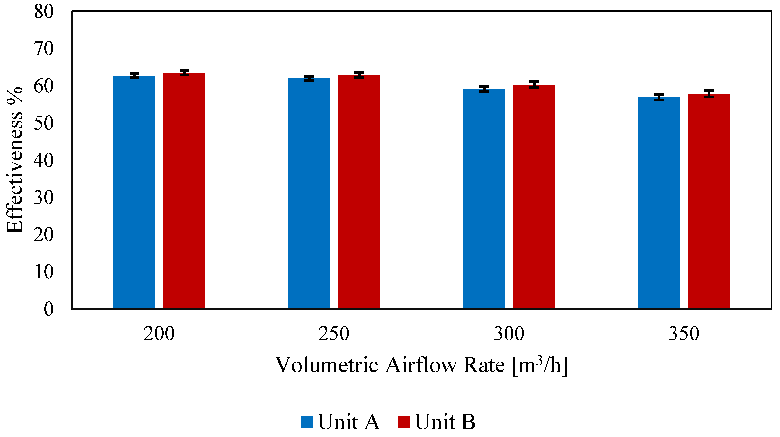
The effectiveness difference between the two HRV units at various flow rates is tabulated in

Table 9. Effectiveness differences between Units A and B at various flow rates.

Flow Rate [m3/h]	ε [%]		Absolute Difference [%]	Percentage Difference [%]	p-Value
	Unit A	Unit B
200	62.7	63.5	0.8	1.3	0.085
250	62.0	62.9	0.9	1.4	0.097
300	59.2	60.3	1.2	2.0	0.047
350	56.9	57.9	1.0	1.7	0.086

and plotted in Figure 13. At a fixed supply inlet temperature of 35 °C, as the airflow rate is increased from 200 to 350 m³/h, the effectiveness for Unit A ranged from 62.7% to 56.9%, while for Unit B it ranged from 63.5% to 57.9%. To determine if these performance differences between the two physically distinct HRV units were statistically significant across the various flow rates, an independent two-sample t-test was performed. The significance level was set at α = 0.05, with a sample size of n = 5 for each HRV unit at each tested condition. A p-value > 0.05 indicates that there is insufficient statistical evidence to conclude that the two units have different performance under the tested conditions. Although no statistically significant differences were observed at most flow rates (p > 0.05), a statistically significant difference was observed at 300 m³/h (p = 0.047). Nevertheless, this difference was small in magnitude, and the differences at the other tested flow rates were not statistically significant. Furthermore, the percentage difference in effectiveness between the two units remained relatively small across all flow rates, ranging from 1.3% to 2.0%. Overall, the results indicate that the two tested units exhibited closely comparable effectiveness under the investigated conditions. Therefore, testing a single unit may provide a sufficiently reliable baseline for preliminary or comparative effectiveness evaluations, although testing additional units would be necessary to characterize broader manufacturing variability.

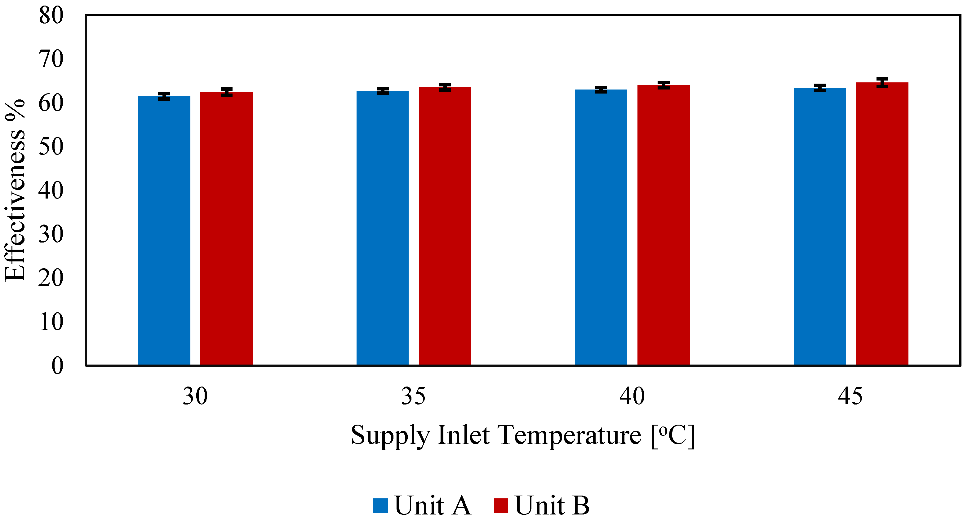
As presented in

Table 10. Effectiveness differences between Units A and B at various supply inlet temperatures.

Supply Inlet Temperature [°C]	ε [%]		Absolute Difference [%]	Percentage Difference [%]	p-Value
	Unit A	Unit B
30	61.5	62.4	0.9	1.5	0.093
35	62.7	63.5	0.8	1.3	0.085
40	63.0	64.0	1.0	1.6	0.129
45	63.4	64.6	1.2	1.9	0.061

and Figure 14, the variations in effectiveness for both HRV units can also be compared at different supply inlet temperatures, with the airflow rate fixed at 200 m³/h. It can be seen that the effectiveness increased with supply inlet temperature for both HRV units, with values ranging from 61.5% to 63.4% for Unit A and from 62.4% to 64.6% for Unit B, as the temperature increased from 30 °C to 45 °C. The percentage differences between the two units under these conditions were again small, ranging from 1.3% to 1.9%. Therefore, within the scope of this evaluation, testing a single unit appears acceptable for comparative effectiveness assessments across the tested temperature range.

4.2.2. Heat Transfer Rate

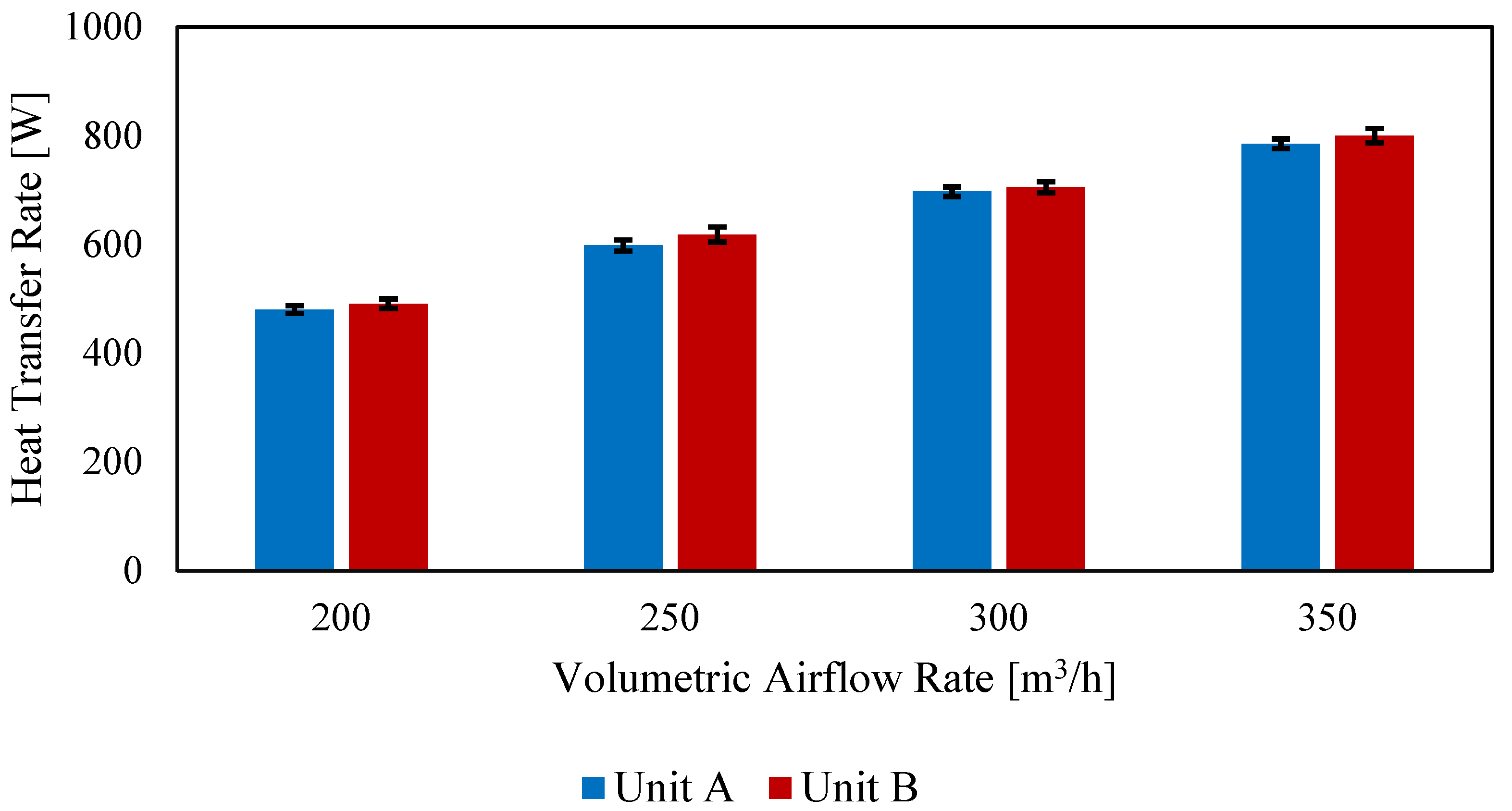
The heat transfer rate comparison between the two HRV units at different airflow rates, with the supply inlet temperature being 35 °C, is presented in

Table 11. Heat transfer rate differences between Units A and B at various flow rates.

Flow Rate [m3/h]	Heat Transfer Rate [W]		Absolute Difference [W]	Percentage Difference [%]	p-Value
	Unit A	Unit B
200	480	491	11	2.3	0.258
250	598	618	20	3.3	0.123
300	697	705	12	1.7	0.261
350	785	800	19	2.4	0.127

and Figure 15. As the airflow rate increases from 200 to 350 m³/h, the heat transfer rate for Unit A ranged from 480 W to 785 W, while Unit B ranged from 491 W to 800 W. The percentage differences in heat transfer rate between the two HRV units remained relatively small across all flow rates, varying between 1.7% and 3.3%. Moreover, none of these differences were statistically significant (p > 0.05). Therefore, the consistent trends indicate that testing a single unit offers a reasonable preliminary baseline for evaluating heat transfer performance under these flow conditions, though assessing additional units would be ideal to fully capture manufacturing tolerances.

Table 12. Heat transfer rate differences between Units A and B at different supply inlet temperatures.

Supply Inlet Temperature [°C]	Heat Transfer Rate [W]		Absolute Difference [W]	Percentage Difference [%]	p-Value
	Unit A	Unit B
30	280	296	16	5.6	0.082
35	480	491	11	2.3	0.258
40	661	678	17	2.5	0.200
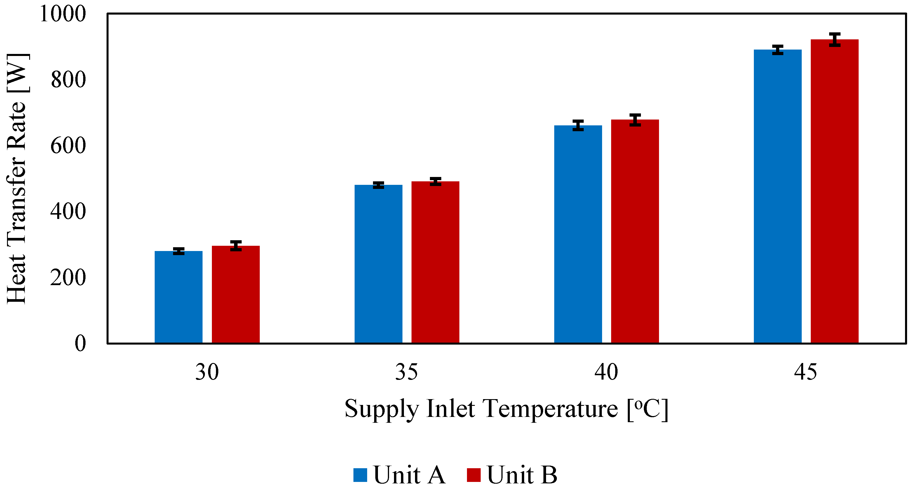
45	890	921	31	3.4	0.109

and Figure 16 show the variation in heat transfer rate for both HRV units at different supply inlet temperatures, with the airflow rate fixed at 200 m³/h. Unit A shows values ranging from 280 W at 30 °C to 890 W at 45 °C, while Unit B ranges from 296 W to 921 W over the same temperature range. The percentage differences in heat transfer rates between the two HRV units range from a low of 2.3% at 35 °C to a high of 5.6% at 30 °C. Statistical analysis shows that the differences in heat transfer between the two HRV units at varying supply inlet temperatures are not statistically significant. Thus, testing with a single unit may provide a reliable representation of heat transfer performance across the temperature range.

4.3. CO₂ Emissions Savings

The annual CO₂ emission reductions were estimated based on the amount of electricity saved by the HRV. To convert the electrical energy savings into avoided carbon emissions, the average electricity emission factor reported by the U.S. Energy Information Administration (EIA) was used. According to the EIA (2023), total U.S. electricity generation from all energy sources produced approximately 0.37 kg CO₂ per kWh of electricity generated. The calculations assumed continuous operation over a 6-month cooling season, corresponding to 180 days/year and 4320 operating hours/year:

$${\mathrm{CO}}_{2,\mathrm{annual}}\left({\displaystyle \frac{\mathrm{k}\mathrm{g}}{\mathrm{y}\mathrm{r}}}\right)=E_{\mathrm{saved}} \left(\mathrm{k}\mathrm{W}\right)\times 0.37 ({\displaystyle \frac{\mathrm{k}\mathrm{g}}{\mathrm{k}\mathrm{W}\mathrm{h}}} )\times 4320 ({\displaystyle \frac{\mathrm{h}}{\mathrm{y}\mathrm{r}}})$$

(10)

Table 13. Annual CO₂ emissions savings with airflow rate for different supply air temperatures.

Volumetric Airflow Rate [m3/h]	Saved CO2 Emissions [kg/yr]
	Tsi = 30 °C	Tsi = 35 °C	Tsi = 40 °C	Tsi = 45 °C
200	151	259	357	481
250	192	323	462	602
300	227	377	537	691
350	246	424	596	776

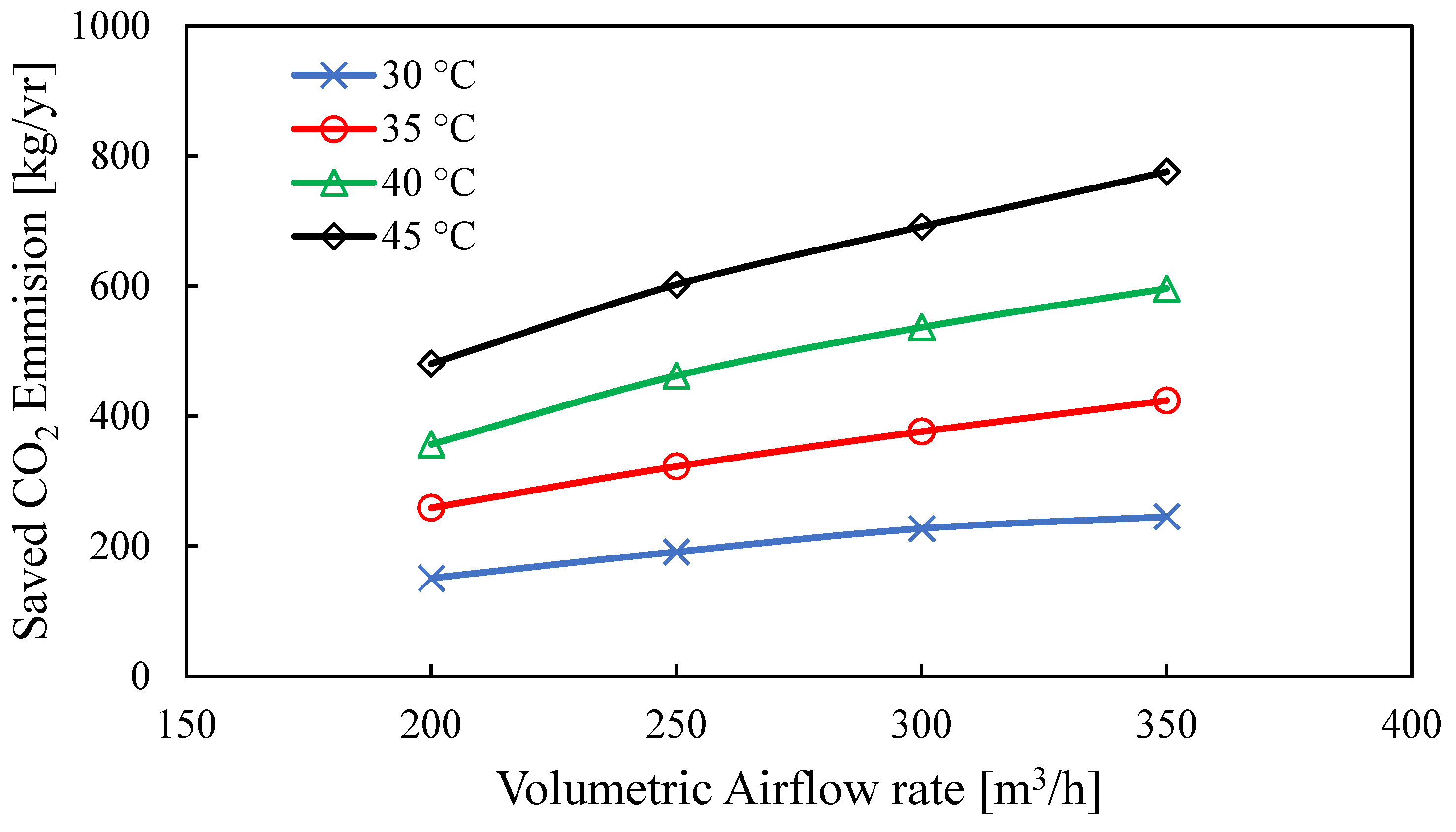
and Figure 17 indicate that both higher supply air temperatures and higher airflow rates improve the amount of recovered energy, leading to greater electricity savings and consequently larger reductions in annual CO₂ emissions. Depending on the operating conditions, the proposed system can avoid between 151 and 776 kg of CO₂ emissions annually.

4.4. Economic Analysis

The economic analysis of the HRV is divided into three parts, namely a simple payback period (PBP), a discounted payback period (DPP), and a net present value (NPV). These three financial indicators provide insight into the profitability of an installed HRV unit and its cost-effectiveness, especially from different perspectives.

The analysis is based on the experimentally measured performance of the HRV unit evaluated in this study. The cost of the HRV unit, based on company pricing, is $1920 including installation, with a lifetime of 25 years. The maintenance cost of the system is estimated at 5% of the total capital cost while the annual interest rate and the inflation rate in electricity prices are taken as 5% and 3%, respectively. The HRV is assumed to operate during a six-month cooling season [21]. Assuming continuous operation (24 h/day), this corresponds to 180 days/year and 4320 operating hours/year. This annual operating period was used to calculate the annual electricity savings, operating cost savings, and payback period.

The HRV unit reduces the cooling load, which in turn leads to electricity savings. This HRV energy savings can be better understood by recalling that the COP for a residential air conditioning is defined as the cooling capacity divided by electrical power consumed by the refrigeration compressor and other primers movers, such as fans. In this context, the COP is used to estimate the amount of electrical energy the A/C system would have consumed to remove the same amount of heat recovered by the HRV. A COP range of 2–4 was selected to represent the typical performance range of conventional air conditioning systems [22]. The electricity saved by operating the HRV in tandem with the A/C can be calculated as follows:

$${\dot{E}}_{saved}={\displaystyle \frac{\dot{Q}}{COP}}-{\dot{P}}_{hrv}$$

(11)

where $\dot{\mathrm{Q}}$ is the heat transfer rate recovered by the HRV and ${\dot{\mathrm{P}}}_{\mathrm{h}\mathrm{r}\mathrm{v}}$ is the power consumed by the HRV. Assuming continuous operation for 4320 h/year, the annual energy savings in kWh can be calculated by multiplying ${\dot{E}}_{\mathrm{s}\mathrm{a}\mathrm{v}\mathrm{e}\mathrm{d}}$ by the annual operating time. To evaluate the financial impact, these energy savings must be translated into cost savings, which is done by multiplying the annual energy savings by the electricity rate.

$${Cost}_{saved}={\dot{E}}_{saved} \times 4320 \times Electricity rate$$

(12)

4.4.1. Simple Payback Period (PBP)

The simple payback period (PBP) represents the time required to recover the initial investment of HRV unit based on annual energy cost savings, without considering the time value of money. PBP provides a quick measure of how quickly the HRV system will recover its initial cost, with shorter payback periods indicating more favorable economic performance. The payback period is given by:

$$PBP={\displaystyle \frac{P_t}{P_i}}$$

(13)

where $P_i$ is the initial investment and $P_t$ is the cashflow, which is determined by using Equation (12).

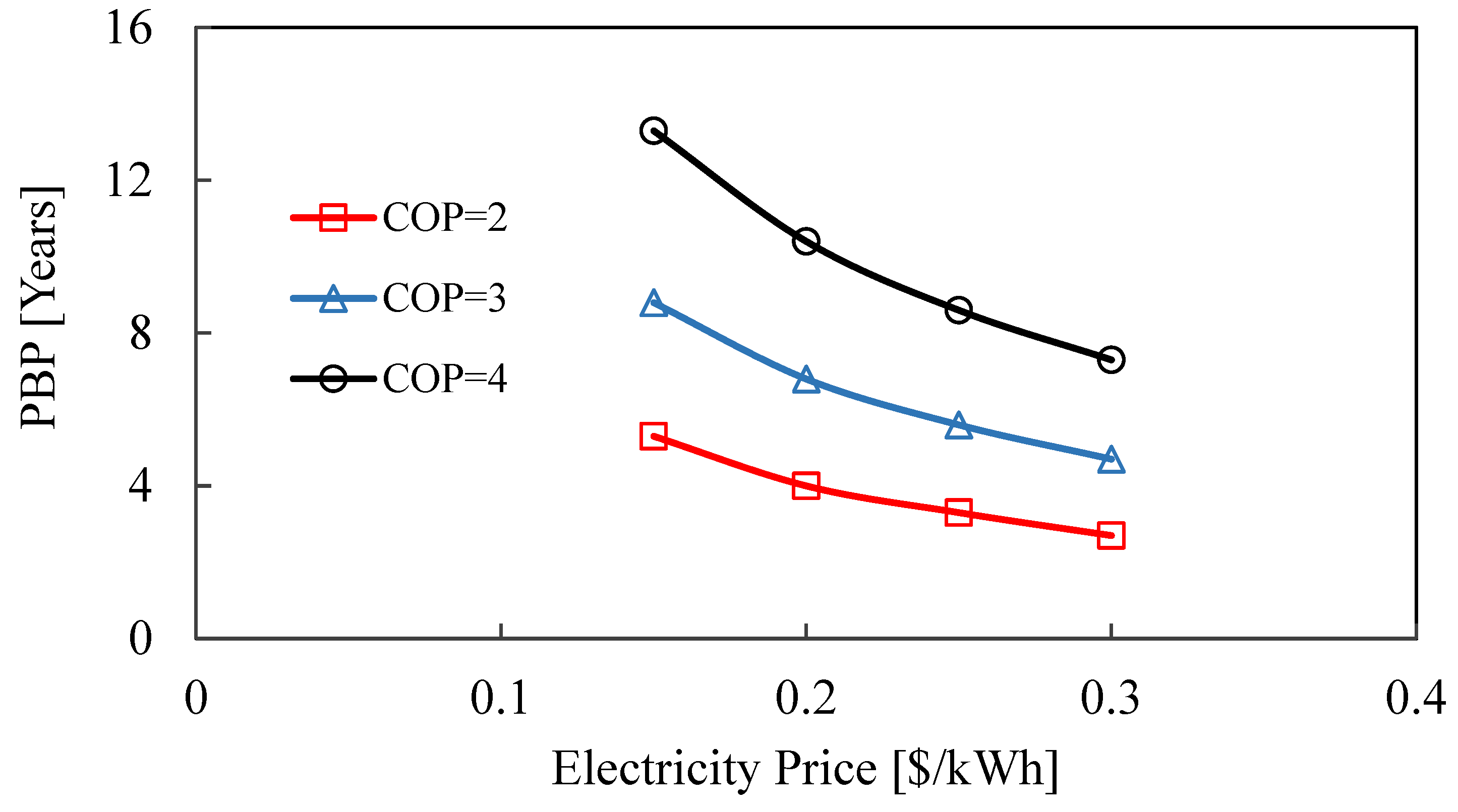
The payback period (PBP) for the HRV unit installed in a building with an A/C operating at various COP values and different electricity prices are tabulated in

Table 14. Simple payback period (PBP) of the HRV unit as a function of COP and electric cost.

COP	$/kWh	PBP [Years]
2	0.15	5.3
	0.20	4
	0.25	3.3
	0.30	2.7
3	0.15	8.8
	0.20	6.8
	0.25	5.6
	0.30	4.7
4	0.15	13.3
	0.20	10.4
	0.25	8.6
	0.30	7.3

. The price of electricity ranged between $0.15 and $0.30/kWh to account for regional differences in electricity tariffs and uncertainty about future energy prices. It can be observed that as the electricity price increases, then the PBP decreases. For example, at COP = 3, as the electricity price increases from 0.15 $/kWh to 0.3 $/kWh, the simple payback period decreases from 8.8 years to 4.7 years. The bottom line is that as energy costs rise then there is a greater need to install and operate HRVs. Also, it can be observed in Table 14 that as the COP decreases then the PBP decreases. For example, at an electricity price of $0.2/kW, a decrease in the COP from 4 to 2 leads to a decrease in the PBP from 10.4 to 4.0 years.

The economic data presented in Table 14 are also plotted in Figure 18, where the aforementioned trends can be easily observed. Lower PBP values in Figure 18 provide a better justification for installing an HRV because of increased energy savings. With this fact in mind, one can see that higher energy costs and A/C with lower COPs are best suited for HRV applications. Additionally, older or less efficient A/C units operate with lower COP, while higher outdoor temperatures further reduce the COP of an A/C unit.

4.4.2. Discounted Payback Period (DPP)

The discounted payback period improves upon the simple method by accounting for the time value of money through a specified discount rate. It determines the time required for the HRV system to recover its initial cost based on the present value of future energy savings. The DPP is given by the following [21]:

$$P_i={\displaystyle \sum _{t=1}^{DPP}}{\displaystyle \frac{P_t}{{(1+i)}^t}}$$

(14)

where i refers to the discount rate and t is the time in years.

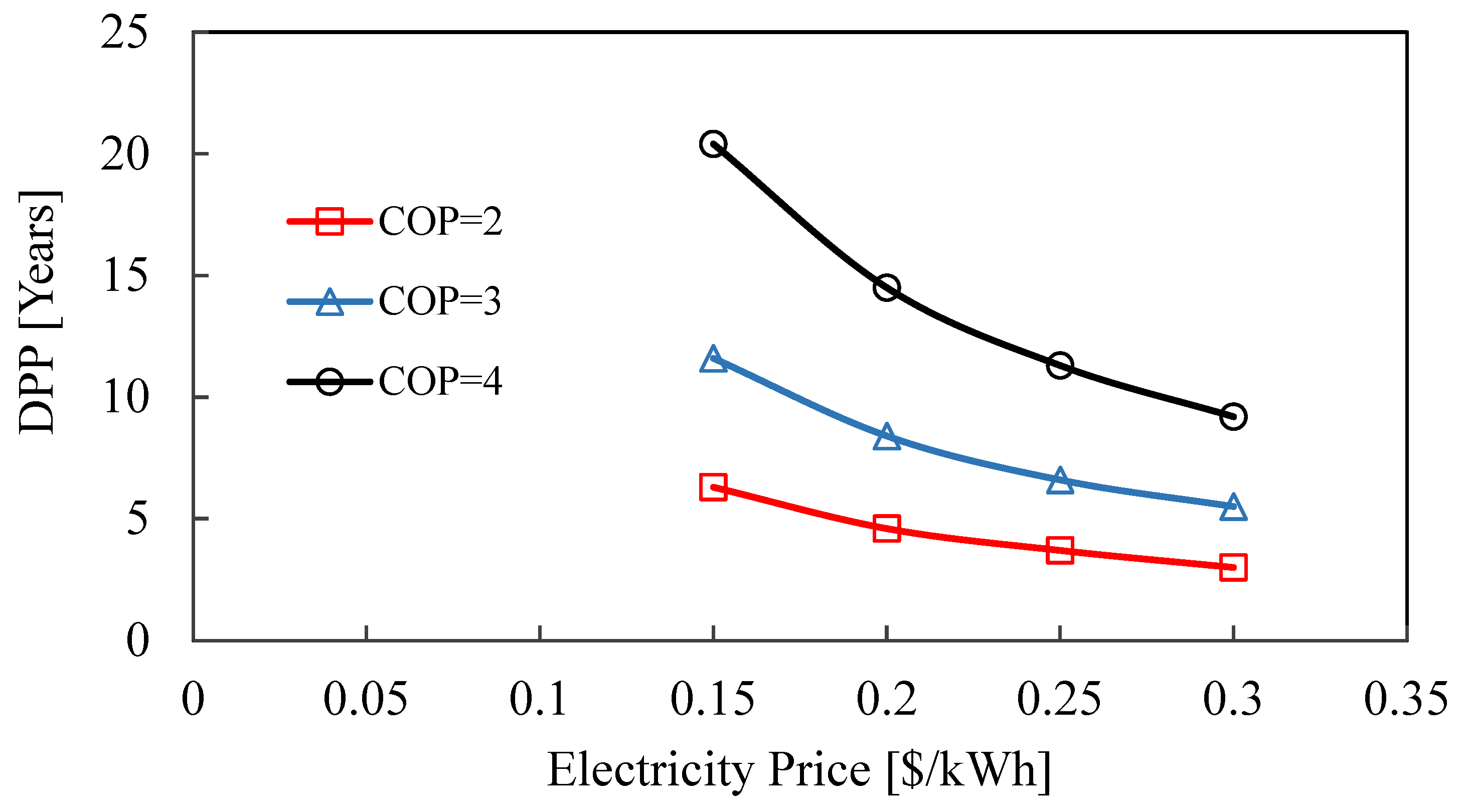
The discounted payback period (DPP) at different COP values and electricity prices are tabulated in

Table 15. Discounted payback period (DPP) of the HRV unit as a function of COP and electric cost.

COP	$/kWh	DPP [Years]
2	0.15	6.3
	0.20	4.6
	0.25	3.7
	0.30	3
3	0.15	11.6
	0.20	8.4
	0.25	6.6
	0.30	5.5
4	0.15	20.4
	0.20	14.5
	0.25	11.3
	0.30	9.2

and then plotted in Figure 19. The trends of the DPP are similar to those of PBP; however, the magnitude of values differ. It can be observed that as electricity prices increase, the DPP decreases, making the HRV installation more desirable. For example, at COP = 3, as the electricity price increases from 0.15 $/kWh to 0.3 $/kWh, the discounted payback period decreases from 11.6 years to 5.5 years. Additionally, it is shown that a decrease in the COP results in lower DPP values. For example, at an electricity price of $0.2/kW, a decrease in the COP from 4 to 2 leads to a decrease in the DPP from 14.5 to 4.6 years.

4.4.3. Net Present Value

The net present value (NPV) represents the total economic benefit of the HRV system over its lifetime by summing the present value of all future energy savings and subtracting the initial investment cost. A positive NPV indicates that the system provides a net financial gain, making it a cost-effective solution. The NPV is given by the following [21]:

$$NPV=-P_i+{\displaystyle \sum _{t=1}^N}{\displaystyle \frac{P_t}{{\left(1+i\right)}^t}}$$

(15)

Table 16. Net present value (NPV) of the HRV unit as a function of COP and electric cost.

COP	$/kWh	NPV [$]
2	0.15	4810
	0.20	7080
	0.25	9350
	0.30	11,630
3	0.15	1850
	0.20	3130
	0.25	4420
	0.30	5700
4	0.15	370
	0.20	1160
	0.25	1950
	0.30	2750

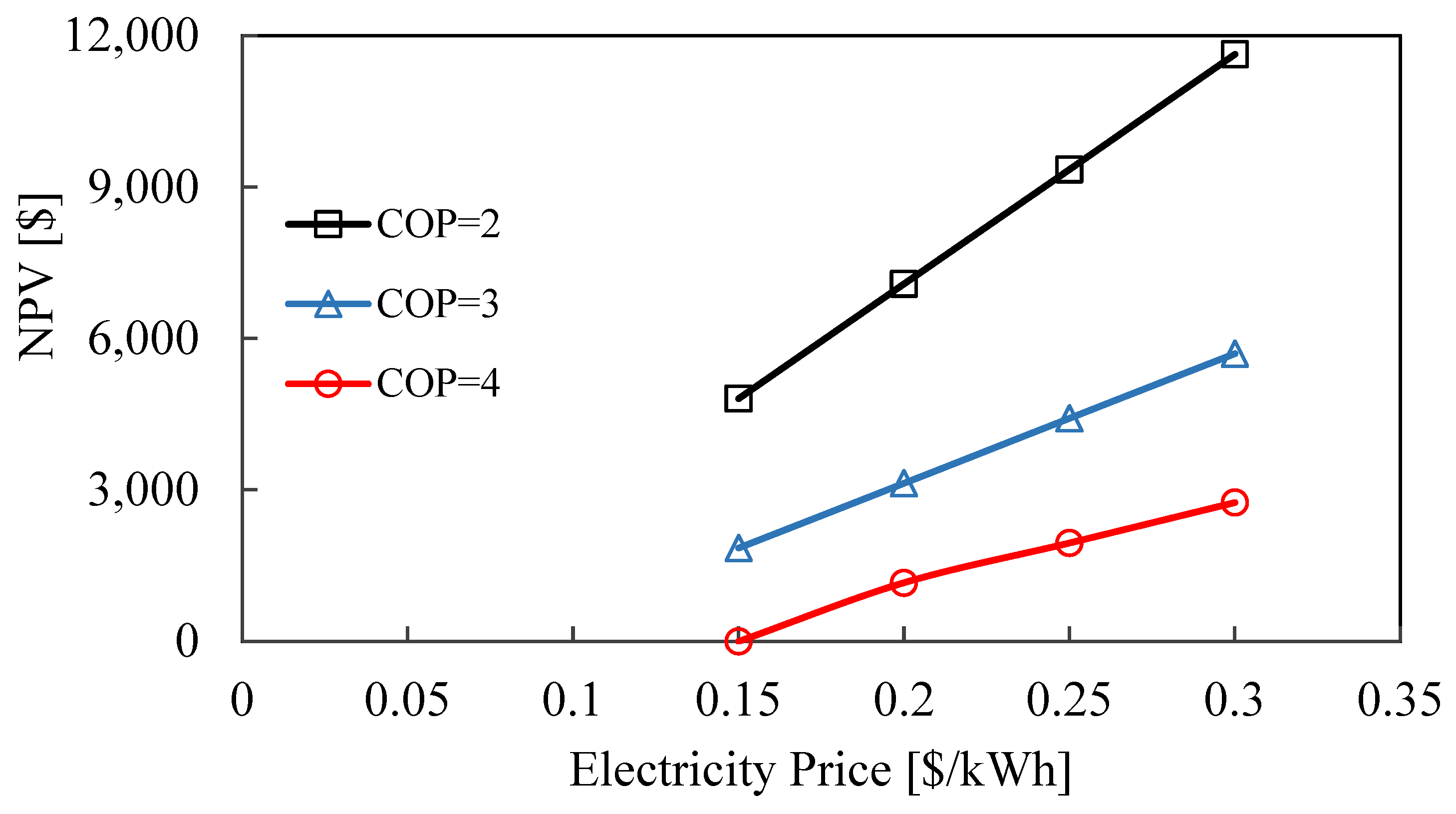
presents the net present value (NPV) for various COP values and electricity prices, with the corresponding trends illustrated in Figure 20. The results show that NPV increases with rising electricity prices. For instance, at a COP of 3, increasing the electricity price from $0.15/kWh to $0.30/kWh increases the NPV from $1850 to $5700. Additionally, as COP increases, the NPV tends to decrease. For example, at an electricity price of $0.20/kWh, decreasing the COP from 4 to 2 results in a significant rise in NPV from $1160 to $7080.

These trends indicate that in residential HVAC systems with lower coefficients of performance (COP), especially in areas with lower electricity costs, the energy savings and economic advantages of using an HRV become more significant, making its implementation more beneficial.

4.4.4. Case Study

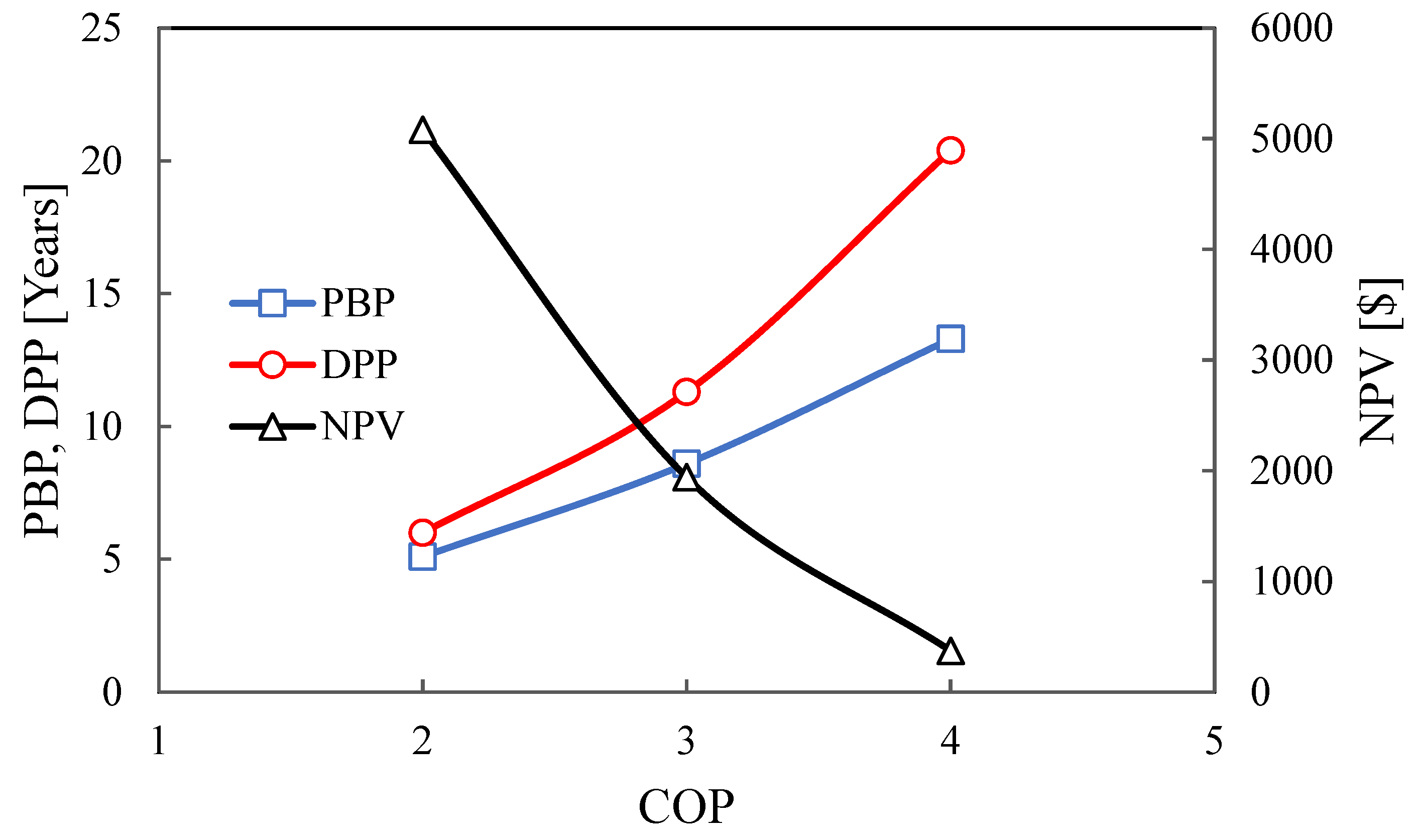
An economic case study was conducted for the US, with PBP, DPP, and NPV values being determined as functions of COP and an average electricity price of 0.17 $/kWh [23], with the results tabulated in

Table 17. PBP, DPP, and NPV at different COP and an average electricity price of US, 0.17 $/kWh.

COP	PBP [Years]	DPP [Years]	NPV [$]
2	5.1	6.0	5082
3	8.6	11.3	1942
4	13.3	20.4	373

and plotted in Figure 21. The best scenario occurs when the net present value (NPV) is highest, and the payback period (PBP) and discounted payback period (DPP) are shortest. This best scenario occurs at the lowest coefficient of performance (COP = 2), which results in an NPV of $5082, a PBP of 5.1 years, and a DPP of 6 years.

5. Conclusions

This experimental study investigates and evaluates thermal, economic, and environmental performances of a residential heat recovery ventilator (HRV). The research addresses a gap in the existing literature by focusing on HRV operations during hot, summer conditions, an area that is often experimentally ignored since residential HRVs are traditionally designed for cold climates. The study assessed the HRV’s thermal performance under varied airflow rates ranging from 200 m³/h to 350 m³/h and supply inlet temperatures between 30 °C and 45 °C, while the economic performance focused on COPs from 2 to 4 and electricity costs from 0.15 $/kWh to 0.3 $/kWh. Experiments were conducted in a testing facility equipped with multiple sensors to measure airflow, temperature, and pressure across the HRV unit. The HRV unit core, with dimensions of 22.8 × 22.8 × 39.4 cm, is configured as a cross-flow, fixed plate-type design.

The study indicates that as the supply inlet temperature increases both effectiveness and heat transfer rate increase. For example, for a flow rate of 200 m³/h, as the supply temperature increases from 30 to 45 °C, the effectiveness rises by 3.1%, and the heat transfer rate increases from 280 W to 890 W. This increase is attributed to the larger temperature difference, which drives the heat exchange process in the HRV. Additionally, increasing the airflow rate from 200 to 350 m³/h results in an increase in the heat transfer rate, due to the higher convective heat transfer coefficient and the greater temperature difference between the hot and cold air. However, the effectiveness decreases. For instance, for a temperature of 35 °C, as the flow rate increases from 200 to 350 m³/h, effectiveness decreases by 10%. This trend is because higher flow rates cause the air to pass through the HRV more quickly, reducing the time available for heat transfer between the incoming and outgoing air streams. Additionally, the U-value increases by 37% when the airflow rate is increased from 200 to 350 m³/h and remain almost constant when the supply inlet temperature increases from 30 °C to 45 °C. The maximum RER of 26.6 Btu/hr.W is obtained for the HRV at 300 m³/h.

To assess repeatability and potential variations in the manufacturing process, the tested unit data were compared to those of a similar unit with the same model number from the same manufacturer. The comparison showed only minor performance differences between both units, with a maximum difference in effectiveness of 2.0%, and heat transfer rate variations ranging from 1.7% to 5.6%.

The economic analysis showed that the addition of an HRV operating in conjunction with a conventional HVAC system becomes less advantageous in regions with lower electricity prices and for HVAC systems with high COPs. For example, at a COP of 2 and an electricity cost of $0.15/kWh, the payback period (PBP) is 5.3 years; however, the PBP increases to 13.3 years at a COP of 4, thereby reducing the economic advantage of the HRV. Similarly, at a COP of 3, reducing electricity prices from $0.30 to $0.15/kWh results in an increase in the PBP from 4.7 to 8.8 years. In addition to achieving favorable economic performance under several operating conditions, the reduction in electricity consumption led to significant environmental benefits, with annual avoided CO₂ emissions ranging from 151 to 776 kg/year.

Further experimental work is recommended to investigate long-term field testing under dynamic outdoor weather conditions to evaluate seasonal degradation and fouling effects on the core. Additionally, extending this experimental methodology to energy recovery ventilators (ERVs) with latent heat recovery would provide a more comprehensive assessment of total cooling load reductions in humid, hot climates.

References

1. Alonso, M.J.; Liu, P.; Mathisen, H.M.; Ge, G.; Simonson, C. Review of heat/energy recovery exchangers for use in ZEBs in cold climate countries. Build. Environ. 2015, 84, 228–237. [Google Scholar] [CrossRef] [Scilit]
2. Qiu, S.; Li, S.; Wang, F.; Wen, Y.; Li, Z.; Li, Z.; Guo, J. An energy exchange efficiency prediction approach based on multivariate polynomial regression for membrane-based air-to-air energy recovery ventilator core. Build. Environ. 2019, 149, 490–500. [Google Scholar] [CrossRef] [Scilit]
3. Belussi, L.; Barozzi, B.; Bellazzi, A.; Danza, L.; Devitofrancesco, A.; Fanciulli, C.; Ghellere, M.; Guazzi, G.; Meroni, I.; Salamone, F.; et al. A review of performance of zero energy buildings and energy efficiency solutions. J. Build. Eng. 2019, 25, 100772. [Google Scholar] [CrossRef] [Scilit]
4. Guillén-Lambea, S.; Rodríguez-Soria, B.; Marín, J.M. Control strategies for Energy Recovery Ventilators in the South of Europe for residential nZEB—Quantitative analysis of the air conditioning demand. Energy Build. 2017, 146, 271–282. [Google Scholar] [CrossRef] [Scilit]
5. Lu, Y.; Wang, Y.; Zhu, L.; Wang, Q. Enhanced performance of heat recovery ventilator by airflow-induced film vibration (HRV performance enhanced by FIV). Int. J. Therm. Sci. 2010, 49, 2037–2041. [Google Scholar] [CrossRef] [Scilit]
6. Wang, M.; Fan, H.; Li, J. Experimental and numerical analysis of a novel air-to-air heat recovery unit based on flat micro-heat pipe array technology for a laboratory animal house. Sci. Technol. Built Environ. 2021, 28, 391–402. [Google Scholar] [CrossRef] [Scilit]
7. Jokisalo, J.; Kurnitski, J.; Vuolle, M.; Torkki, A. Performance of Balanced Ventilation with Heat Recovery in Residential Buildings in a Cold Climate. Int. J. Vent. 2003, 2, 223–236. [Google Scholar] [CrossRef] [Scilit]
8. Yaïci, W.; Ghorab, M.; Entchev, E. Numerical analysis of heat and energy recovery ventilators performance based on CFD for detailed design. Appl. Therm. Eng. 2013, 51, 770–780. [Google Scholar] [CrossRef] [Scilit]
9. Fernández-Seara, J.; Diz, R.; Uhía, F.J.; Dopazo, A.; Ferro, J.M. Experimental analysis of an air-to-air heat recovery unit for balanced ventilation systems in residential buildings. Energy Convers. Manag. 2011, 52, 635–640. [Google Scholar] [CrossRef] [Scilit]
10. Wen, S.; You, R.; Chen, Q. Energy-exergy performance and indoor comfort of a radiant ceiling cooling system with air-to-air sensible heat exchanger in hot and humid climate. Build. Environ. 2026, 290, 114128. [Google Scholar] [CrossRef] [Scilit]
11. Bermejo-Busto, J.; Martín-Gómez, C.; Zuazua-Ros, A.; Baquero, E.; Miranda, R. Performance simulation of heat recovery ventilator cores in cascade connection. Energy Build. 2017, 134, 25–36. [Google Scholar] [CrossRef] [Scilit]
12. Kleszcz, S.; Jaszczur, M.; Pawela, B. An analysis of the periodic counterflow heat exchanger for air-to-air heat recovery ventilators. Energy Rep. 2023, 9, 77–85. [Google Scholar] [CrossRef] [Scilit]
13. Dallaire, J.; Hassan, H.M.A.; Bjernemose, J.H.; Hansen, M.P.R.; Lund, I.; Veje, C.T. Performance analysis of a dual-stack Air-PCM heat exchanger with novel air flow configuration for cooling applications in buildings. Build. Environ. 2022, 223, 77–85. [Google Scholar] [CrossRef] [Scilit]
14. Ra, S.J.; Jo, H.G.; Park, C.S. Real-time model predictive control of energy recovery ventilators for a school building. Sci. Technol. Built Environ. 2025, 31, 1155–1166. [Google Scholar] [CrossRef] [Scilit]
15. Rasouli, M.; Simonson, C.J.; Besant, R.W. Applicability and optimum control strategy of energy recovery ventilators in different climatic conditions. Energy Build. 2010, 42, 1376–1385. [Google Scholar] [CrossRef] [Scilit]
16. Li, B.; Wild, P.; Rowe, A. Performance of a heat recovery ventilator coupled with an air-to-air heat pump for residential suites in Canadian cities. J. Build. Eng. 2019, 21, 343–354. [Google Scholar] [CrossRef] [Scilit]
17. Zhou, F.; Li, D.; Chen, R.; Ma, G. Thermodynamic performance analysis of air-to-air hybrid heat recovery unit driven by pump combined with booster. J. Build. Eng. 2023, 77, 107494. [Google Scholar] [CrossRef] [Scilit]
18. Wang, X.; Wang, Q.; Yoo, S.-J.; Gomyo, T.; Sotokawa, H.; Chung, J.; Kuga, K.; Ito, K. Multi-layered ventilation duct system for heat exchange with air purification. Build. Environ. 2024, 262, 111773. [Google Scholar] [CrossRef] [Scilit]
19. Dieckmann, J.; Roth, K.W.; Brodrick, J. Air-to-air energy recovery heat exchangers. ASHRAE J. 2003, 45, 57–58. [Google Scholar] [CrossRef] [Scilit]
20. Zeng, C.; Liu, S.; Shukla, A. A review on the air-to-air heat and mass exchanger technologies for building applications. Renew. Sustain. Energy Rev. 2017, 75, 753–774. [Google Scholar] [CrossRef] [Scilit]
21. Al-Nimr, M.A.; Mugdadi, B. A hybrid absorption/thermo-electric cooling system driven by a concentrated photovoltaic/thermal unit. Sustain. Energy Technol. Assess. 2020, 40, 100769. [Google Scholar] [CrossRef] [Scilit]
22. Fatouh, M.; Abou-Ziyan, H.; Mahmoud, O.; Abd El-Raheim, D. Experimental analysis of hybrid and conventional air conditioning systems working in hot-humid climate. Appl. Therm. Eng. 2017, 118, 570–584. [Google Scholar] [CrossRef] [Scilit]
23. U.S. Energy Information Administration. Electric Power Monthly: Table 5.3. 2026. Available online: https://www.eia.gov (accessed on 1 August 2026).
Figure 1. Test rig schematic with ducting, sensors, and core (red—supply airflow; blue—exhaust airflow).
Cleantechnol 08 00133 g001
Figure 2. HRV core showing supply air (red) from the outdoors and exhaust air (blue) from the building space.
Cleantechnol 08 00133 g002
Figure 3. The impact of volumetric flow rate on the HRV heat transfer rate for Tsi = 35 °C.
Cleantechnol 08 00133 g003
Figure 4. The impact of supply inlet temperature on HRV heat transfer rate for V ˙ = 200 m3/h.
Cleantechnol 08 00133 g004
Figure 5. The impact of flow rate on HRV heat transfer for a range of supply inlet temperatures.
Cleantechnol 08 00133 g005
Figure 6. The impact of supply inlet temperature on HRV heat transfer for a range of flow rates.
Cleantechnol 08 00133 g006
Figure 7. The impact of flow rate on HRV effectiveness (solid lines) and exergy efficiency (dashed lines) for a range of supply inlet temperatures.
Cleantechnol 08 00133 g007
Figure 8. The impact of supply inlet temperature on HRV effectiveness (solid lines) and exergy efficiency (dashed lines) for a range of flow rates.
Cleantechnol 08 00133 g008
Figure 9. The impact of flow rates on U-value for a range of supply inlet temperatures.
Cleantechnol 08 00133 g009
Figure 10. The impact of supply inlet temperature on the U-value for a range of flow rates.
Cleantechnol 08 00133 g010
Figure 11. The impact of flow rate on recovery efficiency ratio for a range of supply inlet temperatures.
Cleantechnol 08 00133 g011
Figure 12. The impact of supply inlet temperature on Recovery efficiency ratio for a range of flow rates.
Cleantechnol 08 00133 g012
Figure 13. Effectiveness differences between units at various flow rates for a supply inlet temperature of 35 °C with error bars shown.
Cleantechnol 08 00133 g013
Figure 14. Effectiveness differences between units at various supply inlet temperatures for flow rate of 200 m3/h with error bars shown.
Cleantechnol 08 00133 g014
Figure 15. Heat transfer rate differences between units at various flow rates for supply inlet temperature of 35 °C with error bars shown.
Cleantechnol 08 00133 g015
Figure 16. Heat transfer rate differences between units at various supply inlet temperatures for a flow rate of 200 m3/h with error bars shown.
Cleantechnol 08 00133 g016
Figure 17. Variation of annual CO2 emissions savings with airflow rate for different supply air temperatures.
Cleantechnol 08 00133 g017
Figure 18. The simple payback period (PBP) at different COPs and electricity prices.
Cleantechnol 08 00133 g018
Figure 19. The discounted payback period (PBP) at different COPs and electricity prices.
Cleantechnol 08 00133 g019
Figure 20. The net present value at different COPs and electricity prices.
Cleantechnol 08 00133 g020
Figure 21. Case study: the payback period (PBP), discounted payback period (DPP), and net present value (NPV) at different COPs for an assumed average electricity price of US, 0.17 $/kWh.
Cleantechnol 08 00133 g021