Adaptive Energy Stations for Sustainable Transport Infrastructure: Real-Time Dispatch Optimization Using Marginal Grid Emissions and Low-Carbon Fuel Pathways

Abstract

Transport decarbonization requires infrastructure that can use time-resolved carbon information without overstating the representativeness of short proof-of-method runs. This study introduces Adaptive Energy Stations (AESs), multi-fuel transport-energy nodes that integrate marginal grid-emission signals, fuel life-cycle carbon intensities, wholesale electricity prices, and vehicle operating constraints into a station-level dispatch optimization. The implemented case is a one-week winter proof-of-method for CAISO/CAISO_NORTH using 168 hourly service events over 1–8 January 2026 Pacific time, archived WattTime marginal operating emissions, CAISO locational marginal prices, eGRID CAMX annual-average factors, and declared vehicle and fuel-pathway parameters. In the audited CAISO scenario, the attached dispatch outputs report a reduction from 181.76 to 123.38 g CO₂e/km relative to the specified static baseline, corresponding to a 32.12% reduction for the one-week winter service-event stream. The populated dispatch trace shows that the carbon-priority AES plug-in hybrid electric vehicle (PHEV) run selected cellulosic E85 for all 168 events and selected no electric events; this result is interpreted as an operational scenario result for the archived week, not as an annual fleet-average, smart-charging benefit, or deployment forecast. The revised analysis explicitly separates implemented CAISO evidence from ERCOT, MISO-MROW, and ISO–NE extension sensitivities, which remain hypothetical until equivalent marginal-emissions, price, and service-event data are supplied. Battery-production amortization is treated as a separate sensitivity because it can change battery electric vehicle (BEV)–cellulosic E85 equivalence conclusions: at 50–100 kg CO₂e/kWh over 240,000 km, a 75 kWh BEV pack contributes 15.6–31.3 g CO₂e/km and a 14 kWh PHEV pack contributes 2.9–5.8 g CO₂e/km. Practical-equivalence claims are therefore conditional on the declared boundary, equivalence margin, and production-emissions treatment. Full deployment requires validated marginal-emission access, transparent dispatch-audit outputs, supply-chain verification, user-behavior characterization, cost sensitivity analysis, and cybersecurity safeguards.

1. Introduction

Decarbonizing road transport demands coordinated advances in vehicle technology, fuel supply chains, and energy infrastructure. Life-cycle assessment (LCA) has become the standard tool for comparing vehicle-energy pathways, yet most published comparisons rely on annual-average grid emission factors and fixed fuel-pathway assumptions [1]. While such static analyses are indispensable for identifying promising technology directions, they cannot resolve the temporal variability that governs real-world charging and refueling decisions. A battery electric vehicle (BEV) charged during a midday solar surplus in California may produce substantially fewer life-cycle emissions than the same vehicle charged during an evening fossil-fuel ramp—a distinction invisible to annual-average accounting. Conversely, a low-carbon biofuel may offer an immediate emission advantage in regions or hours where grid decarbonization has not yet displaced marginal fossil generation.

This temporal dimension has received growing attention in the smart-charging literature. Graff Zivin et al. [2] demonstrated that the environmental benefit of electricity-shifting policies depends on the marginal generator displaced, not the system average. Holland et al. [3] showed that local grid composition can reverse the emission ranking of electric vehicles relative to conventional alternatives. These findings imply that infrastructure-level decisions—when to charge, which fuel to dispense, and how to advise drivers—require time-resolved carbon information rather than static pathway comparisons alone.

The present study addresses this gap by developing an Adaptive Energy Station (AES) framework. An AES is conceived as a multi-fuel transport-energy node that integrates electric charging infrastructure with low-carbon liquid-fuel dispensing, and that uses real-time marginal grid-emission signals, fuel life-cycle carbon intensities, wholesale electricity prices, vehicle operating constraints, and user preferences to select the lowest-emission feasible energy pathway at each service event. The concept extends earlier work on bifuel-vehicle LCA modeling in Brazil, where flexible liquid-fuel selection was framed as an environmental optimization problem [4], to a station-level decision architecture that also incorporates electrification and time-varying grid carbon intensity.

The contribution is infrastructure-centered rather than vehicle-centered. The objective is not merely to compare BEV and biofuel pathways under static assumptions, but to operationalize life-cycle carbon information in transaction-level station decisions—bridging the gap between pathway-level LCA and real-time energy management.

To situate the proof-of-method result relative to published vehicle-LCA comparisons, recent EV–ICE studies generally report that BEV life-cycle advantages depend strongly on electricity mix, battery-production assumptions, lifetime mileage, vehicle class, and system-boundary choices rather than tailpipe emissions alone [5,6,7,8,9,10,11]. The AES result is therefore compared with those studies as a station-level dispatch outcome for a declared PHEV service stream, not as a new vehicle-fleet LCA ranking.

To maintain scientific rigor, the study explicitly separates implemented evidence from prospective extension cases. The executable proof-of-method is demonstrated for the California Independent System Operator (CAISO) zone using 168 hourly service events spanning one winter week, 1–8 January 2026 Pacific time. The CAISO case uses archived WattTime CAISO_NORTH marginal operating-emissions records as historical API data for the completed interval, not as model-generated forecasts or synthetic emissions; the reproducibility archive must retain the query window, retrieval date, endpoint identifier, row counts, units, and checksums. CAISO locational marginal prices supply the economic component. Three additional U.S. grid zones—ERCOT, MISO-MROW, and ISO–NE—are defined only as extension sensitivity cases. Their numerical values should be read as hypothetical model explorations, not empirical regional dispatch reductions, until equivalent marginal-emission access, zone-specific price data, documented eGRID crosswalks, and region-appropriate service-event inputs are supplied.

The study addresses four research questions:

• To what extent does AES temporal and multi-fuel dispatch reduce PHEV emissions relative to a fully specified static strategy in the implemented CAISO case?
• How do multi-zone extension sensitivity cases behave when the same model structure is applied with region-specific average grid factors and scenario inputs?
• Under the stated scenario uncertainty model, are CAISO-zone BEV and cellulosic E85 life-cycle emissions practically equivalent within predefined margins, and how does this conclusion change when battery-production emissions are amortized explicitly?
• Do PHEVs provide operational flexibility advantages relative to BEV-only or E85-only operation, and which policy interpretations remain conditional on user behavior, fuel availability, cost weights, and seasonal representativeness?

The remainder of this paper is organized as follows. Section 2 reviews the literature on LCA uncertainty quantification, marginal-emissions methodology, PHEV charging behavior, biofuel carbon intensity, time-dependent charging, battery-production effects, and computational reproducibility. Section 3 describes the methodology, including the LCA scope, data provenance, optimization formulation, and uncertainty propagation. Section 4 presents results for the CAISO proof-of-method case and multi-zone sensitivity analyses. Section 5 discusses implications for transport decarbonization policy, regional deployment, and framework limitations. Section 6 states the main conclusions.

2. Literature Review

2.1. Life Cycle Assessment and Uncertainty Quantification in Transportation Systems

Life cycle assessment (LCA) remains the standard methodology for evaluating transportation technologies across fuel production, vehicle manufacturing, operation, and end-of-life stages [1,12]. Recent EV–ICE LCA reviews and comparative studies emphasize that conclusions depend strongly on the electricity mix, battery-production intensity, lifetime mileage, vehicle mass, and allocation assumptions [6,11,13,14,15,16,17]. This literature supports the present manuscript’s decision to avoid interpreting a one-week station-level dispatch output as a universal vehicle-technology ranking.

Several recent studies compare electric vehicles directly with fossil-fuel-powered cars. Tang et al. [7], Kurkin et al. [8], Vieira et al. [9], and Malik et al. [10] each show that BEV advantages are sensitive to grid carbon intensity and battery assumptions, while Bieker [5] reports broad regional BEV life-cycle benefits under current and projected electricity mixes. Other work highlights regional or use-case specificity, including charging hubs [18], shared and automated electric mobility [19], green logistics [20], consequential use-phase non-linearities [21], and national or regional scenarios [22,23,24,25]. The present AES model differs from these studies by optimizing transaction-level station choices for PHEVs and fuel pathways rather than comparing fixed vehicle archetypes alone.

The present AES framework implements 10,000 Monte Carlo draws with documented pseudo-random seeds and Latin hypercube sampling options. The uncertainty intervals are scenario-propagation intervals rather than statistical confidence intervals from a field sample. This distinction is important because the 168 CAISO service events demonstrate an auditable proof-of-method calculation chain, not a population-weighted annual transport dataset.

2.2. Marginal Emissions Factors and Time-Resolved Grid Carbon Intensity

A fundamental methodological debate in electric vehicle LCA concerns whether to use average or marginal emissions factors when attributing grid carbon intensity to charging events. Average emissions factors represent the carbon intensity of the entire generation mix, while marginal emissions factors represent the carbon intensity of the specific generator that ramps up or down in response to incremental load changes [2,26]. This distinction has profound implications for EV environmental assessment and charging optimization strategies.

Holland et al. [3] demonstrated that the environmental benefits of electric vehicles vary dramatically by location due to regional differences in marginal generation sources, with EVs in coal-heavy regions potentially producing higher emissions than efficient gasoline vehicles. Their spatially explicit analysis revealed that using average emissions factors systematically overestimates EV benefits in regions where fossil-fueled peaker plants respond to marginal load increases.

The temporal dimension of marginal emissions has been rigorously examined in the recent literature. Graff Zivin et al. [2] quantified spatial and temporal heterogeneity in marginal emissions across U.S. regions, demonstrating that electricity-shifting policies (including EV charging schedules) must account for hour-by-hour variation in grid dispatch to accurately estimate emissions impacts. Miller et al. [26] developed an hourly accounting framework for electricity consumption emissions, showing that charging an EV in solar-rich California during midday produces 70% lower emissions than overnight charging, while the pattern reverses in regions with substantial nuclear or hydroelectric baseload generation.

WattTime [27] provided empirical evidence from CAISO operations demonstrating that marginal emissions rates can exceed average rates by a factor of three during high-demand periods, even when renewable penetration is substantial. Their analysis revealed that a CAISO charging event during a 50% renewable supply period could trigger a marginal response from an inefficient gas peaker at 927 lbs CO₂/MWh, far exceeding the 283 lbs CO₂/MWh average rate. This distinction supports the present study’s use of marginal emissions for dispatch decisions and average emissions for static-baseline comparison.

The present AES framework operationalizes marginal emissions methodology by incorporating time-indexed CAISO_NORTH marginal operating emissions data into the dispatch optimization. The use of marginal emissions here should be understood as an operational dispatch signal rather than a claim that the full study is a consequential LCA. The LCA inventory and pathway-comparison boundary remain attributional, while marginal MOER values are used to screen incremental station-level charging actions. Large-scale market-mediated effects—such as changes in electricity investment, ethanol demand, land use, or grid congestion—are identified as future consequential-LCA extensions rather than included in the implemented proof-of-method.

2.3. Plug-In Hybrid Electric Vehicle Utility Factors and Real-World Charging Behavior

The utility factor (UF)—defined as the fraction of vehicle kilometers traveled in charge-depleting mode—is a critical parameter for assessing PHEV environmental performance. The SAE J2841 standard [28] provides a methodology for estimating UF based on vehicle all-electric range and assumed daily charging behavior, but empirical studies show that real-world PHEV electric driving can differ substantially from standardized assumptions.

Plötz et al. [29] reported large gaps between type-approval and real-world PHEV fuel consumption across China, Europe, and North America, with lower electric driving shares when charging is infrequent. More recent PHEV utility-factor work has emphasized the need to represent heterogeneous charging behavior and habitual non-charging explicitly [30]. These findings are directly relevant to AES operation: a station-level recommendation can reduce emissions only when drivers, charging opportunities, state of charge, fuel availability, and trip requirements allow the recommended action to be followed.

The present AES framework incorporates these insights by modeling PHEV service events with declared utility-factor assumptions that should be replaced by fleet-specific charging-behavior data before deployment assessment. The framework’s hourly dispatch optimization accounts for electricity prices, grid carbon intensity, and user preferences—factors absent from static UF calculations.

2.4. Biofuel Life Cycle Assessment and Cellulosic Ethanol Pathways

The environmental performance of biofuels depends on feedstock type, production pathway, land-use treatment, refinery energy, coproduct treatment, and distribution logistics. GREET-style well-to-wheels modeling remains a central reference for U.S. fuel-pathway accounting [1,12], and earlier ethanol LCA work established that corn, sugarcane, and cellulosic pathways can differ substantially in greenhouse-gas performance [31]. Recent comparative reviews also emphasize that biofuel and electricity pathways should be interpreted with explicit regional and supply-chain boundaries [11,16,32].

The present AES framework represents liquid-fuel pathways through declared well-to-wheels carbon-intensity factors rather than separate process modules. The proof-of-method implementation uses 25 g CO₂eq/MJ for cellulosic E85 as a scenario pathway and compares it with corn E85, E10, and gasoline reference values. These values are scenario inputs; deployment assessment requires replacement with region- and supply-chain-specific LCA records that account for feedstock sourcing, refinery efficiency, transportation logistics, coproduct markets, certification, and station inventory.

2.5. Time-Dependent Emissions and Smart Charging Strategies

The temporal variability of grid carbon intensity creates opportunities for emissions reduction through intelligent charging strategies that shift electricity demand to low-carbon periods. Miller et al. [26] demonstrated that EV charging time-of-day decisions have first-order effects on lifecycle emissions, with midday charging in California producing 70% lower emissions than overnight charging due to solar generation displacement of fossil peakers. Their analysis revealed that “evening charging is the worst, highest-emission time to charge in nearly all states,” while overnight charging is cleanest in regions with substantial wind or nuclear baseload capacity.

The present AES framework operationalizes these insights by incorporating hourly electricity prices and marginal emissions factors into a dispatch optimization that selects between electric charging and low-carbon liquid fuel based on real-time grid conditions. This approach extends beyond passive smart charging (which shifts EV load to low-carbon periods) to active fuel-switching for PHEVs, enabling vehicles to avoid high-carbon grid intervals entirely by operating in charge-sustaining mode with cellulosic ethanol.

2.6. Battery Production and Vehicle Manufacturing Impacts

Battery production can materially affect vehicle life-cycle comparisons, particularly when electricity used in cell manufacturing is carbon intensive or when lifetime mileage is low. Recent reviews and battery-focused LCAs identify battery chemistry, manufacturing electricity, battery lifetime, capacity fade, recycling, second-life treatment, physical recycling, and next-generation cell design as key drivers of BEV and PHEV production impacts [33,34,35,36,37,38,39,40,41,42,43,44,45]. Vehicle lightweighting, battery-enclosure design, and alternative vehicle architectures can further shift life-cycle results [46,47,48].

The present AES framework separates two questions that are often conflated. For transaction-level dispatch of an already arriving vehicle, vehicle and battery production terms are fixed with respect to the immediate choice between charging and liquid-fuel operation, so they do not determine the selected action. For technology-pathway comparison, however, manufacturing cannot be ignored. The revised analysis therefore reports battery-production amortization as an explicit sensitivity and avoids interpreting the operational dispatch result as a full vehicle-technology ranking unless production terms and lifetime assumptions are included.

2.7. Computational Reproducibility in Energy Systems Research

Computational energy-system results are difficult to evaluate when code versions, input files, time stamps, units, and data transformations are not archived. The present study therefore treats reproducibility artifacts as part of the scientific evidence rather than as optional supporting documentation. The archive is designed to contain source code, input CSV files, output CSV files, figure-generation scripts, checksums, random seeds, package versions, and a data dictionary that identifies whether each input is measured, source-derived, or scenario-declared.

The present study operationalizes these principles by committing to archive: (i) source code for the AES dispatch model and Monte Carlo uncertainty propagation; (ii) CAISO/CAISO_NORTH input tables used for the 1–8 January 2026 proof-of-method run; (iii) figure-generation scripts; (iv) CSV files used to generate tables and figures; (v) a README with exact commands, package versions, random seeds, and units; and (vi) a data dictionary identifying which entries are measured, source-derived, or scenario inputs. A permanent public DOI will be inserted before journal submission, enabling independent verification and extension to additional grid regions (ERCOT, MISO-MROW, ISO–NE) as marginal-emissions and public-agency data become available.

2.8. Research Gaps and Contribution of the Present Study

The reviewed literature establishes that: (1) Monte Carlo uncertainty propagation is essential for robust LCA conclusions but is rarely applied to real-time infrastructure dispatch; (2) marginal emissions factors are better suited than annual averages for incremental charging-dispatch decisions, yet most EV charging infrastructure ignores real-time grid signals; (3) real-world PHEV charging behavior deviates substantially from standardized assumptions, creating opportunities for adaptive dispatch that accounts for actual usage patterns; (4) biofuel pathways can achieve low greenhouse-gas intensities but exhibit high variability depending on feedstock, coproduct treatment, and supply-chain certification; (5) time-dependent grid carbon intensity creates opportunities for smart charging optimization, but existing frameworks focus mainly on BEVs rather than multi-fuel vehicles; and (6) computational reproducibility requires comprehensive archiving of code, data, and environment specifications.

However, existing studies have not integrated these insights into an operational framework that combines time-resolved marginal emissions, liquid-fuel pathway carbon intensity, vehicle constraints, and user preferences to guide transaction-level infrastructure decisions. Static LCA comparisons cannot determine when a PHEV should charge versus operate on low-carbon liquid fuel, nor can they optimize station-level dispatch across heterogeneous vehicle fleets with varying charging needs and fuel preferences. Smart charging frameworks for BEVs cannot accommodate vehicles with liquid-fuel range extension, while biofuel LCA studies do not incorporate real-time grid conditions into fuel selection decisions.

The present study addresses this gap by developing an Adaptive Energy Station (AES) framework that operationalizes lifecycle carbon information in real-time dispatch decisions for multi-fuel vehicle infrastructure. The contribution is threefold:

Methodological: The AES framework integrates Monte Carlo uncertainty propagation with time-resolved marginal emissions and liquid-fuel pathway LCA, distinguishing measured data from scenario inputs and quantifying the sensitivity of emissions reductions to parameter assumptions. This approach extends LCA methodology from static technology comparison to dynamic operational optimization.

Infrastructure-centered: Rather than comparing BEV and biofuel pathways under static assumptions, the AES framework enables stations to dynamically select the lowest-carbon energy option based on current grid conditions, fuel availability, vehicle state, and user preferences. This shifts the analytical focus from vehicle technology choice to infrastructure dispatch strategy, recognizing that multi-fuel vehicles create optimization opportunities unavailable to single-fuel platforms.

Reproducible: The framework implements comprehensive documentation and archiving practices advocated by the computational reproducibility literature, including version-controlled code, SHA-256 checksums, machine-readable uncertainty tables, and a data dictionary that categorizes all inputs by source type. This enables independent verification, sensitivity analysis with alternative assumptions, and extension to additional grid regions and fuel pathways.

The proof-of-method implementation for CAISO/CAISO_NORTH demonstrates that the AES calculation chain can execute with time-resolved marginal-emissions and price data and can alter transaction-level energy selections relative to a static baseline. The magnitude of the reported reduction remains conditional on the one-week winter interval, the declared service-event stream, the static-baseline definition, the availability of cellulosic E85, and the dispatch-audit outputs. The framework provides infrastructure operators with decision support that adapts to real-time conditions while maintaining transparency about the assumptions and uncertainties that affect emissions estimates.

3. Methods

3.1. Goal, Scope, Functional Unit, and Scenarios

The assessment compares light-duty vehicle energy pathways within an attributional LCA framework aligned with ISO 14040/14044 principles [49,50]. The functional unit is one vehicle-kilometer traveled, chosen because it normalizes energy consumption and emissions across powertrains with fundamentally different energy carriers. System boundaries encompass vehicle production (including battery manufacturing for electrified powertrains), fuel or electricity production through well-to-wheels or well-to-plug pathways, use-phase energy consumption, and end-of-life allocation. Charging-station and ethanol-dispenser construction are excluded from the vehicle-kilometer functional unit; these infrastructure elements are treated as deployment constraints and identified as requirements for future consequential-LCA extensions.

For clarity, the study distinguishes the dispatch boundary from the pathway-comparison boundary. The dispatch boundary concerns a vehicle already present at a station; production emissions are constant across feasible actions for that vehicle and therefore do not affect the immediate electric-versus-liquid action choice. The pathway-comparison boundary compares BEV, PHEV, and liquid-fuel pathways; in that boundary, battery-production amortization is reported explicitly because different battery sizes can materially change BEV–E85 equivalence conclusions. This distinction prevents the operational AES result from being misread as a complete vehicle-technology LCA ranking.

The scenario framework spans four U.S. grid zones (

Table 1. Grid-zone definitions and implementation status.

Scenario Identifier	Operational Grid Zone for Marginal Dispatch Data	Static-LCA Average Factor	Status in This Study	Interpretation
CAISO	WattTime CAISO_NORTH/California Independent System Operator	eGRID CAMX	Implemented proof-of-method run	Reproducible one-week CAISO case
ERCOT	Electric Reliability Council of Texas	eGRID ERCT	Extension sensitivity case	Requires equivalent marginal-emissions access
MISO–MROW	MISO Midwest proxy	eGRID MROW	Extension sensitivity case	Requires exact marginal zone and eGRID crosswalk
ISO–NE	ISO New England	eGRID NEWE	Extension sensitivity case	Requires equivalent marginal-emissions access

Sources for Table 1 are reported in the surrounding text: EPA eGRID for average factors, WattTime documentation for marginal-emissions signals, and CAISO OASIS documentation for the implemented price stream [51,52,53,54].

): CAISO, ERCOT, MISO-MROW, and ISO–NE. Each zone is characterized by two complementary emission metrics: a marginal operating emissions rate for time-resolved AES dispatch, and an annual-average emission factor from the EPA’s Emissions and Generation Resource Integrated Database (eGRID) for static-baseline comparison [51]. This dual-metric approach is deliberate—marginal rates capture the carbon intensity of the generator actually displaced by an incremental charging load, while annual averages represent the system-wide emission intensity used in conventional LCA.

Only the CAISO zone constitutes an implemented proof-of-method case. CAISO uses WattTime CAISO_NORTH marginal operating emissions data for dispatch and is mapped to eGRID subregion CAMX for annual-average factors. The remaining three zones are retained as explicitly defined extension cases: ERCOT maps to eGRID ERCT, MISO-MROW to eGRID MROW, and ISO–NE to eGRID NEWE. These extension zones are analyzed using the same model structure with region-specific average grid factors and scenario inputs, but they should not be interpreted as completed real-data dispatch runs. Promoting them to implemented status requires equivalent marginal-emission access, corresponding wholesale price data, documented eGRID crosswalks, and source-specific service-event inputs.

Table 2. Data streams, model role, and evidence status.

Input Class	Role in Model	Status for CAISO Run	Status for Extension Zones
Marginal operating emissions	Time-varying electricity carbon intensity for AES dispatch	CAISO_NORTH time series used for the one-week run	Required before empirical regional dispatch claims
Electricity price	Time-varying cost component for charging decisions	CAISO hourly proxy used	Required for each zone
eGRID average factor	Static baseline electricity carbon intensity	CAMX factor used	ERCT, MROW, and NEWE factors used only in sensitivity framing
Liquid-fuel pathway carbon intensity	Carbon intensity of E85, E10, and gasoline pathways	Scenario pathway values used	Same pathway values used unless region-specific supply chains are added
Liquid-fuel prices	Cost component for fuel decisions	Hourly or repeated price rows used in the input archive	Zone-specific fuel-price data required
Vehicle parameters	Energy use, battery capacity, and production-emissions allocation	PHEV and BEV scenario parameters used	Same unless region- or fleet-specific vehicles are introduced
Service events	Demand instances and timestamps	168 hourly events, 1–8 January 2026	Region-specific station or fleet observations required

The table serves as an audit map: only the CAISO/CAISO_NORTH column set represents executable, validated evidence. Other regions are sensitivity cases until the corresponding marginal-emissions, price, and service-event data are supplied.

classifies each input stream by its role in the model and its evidence status. Static annual electricity factors draw on eGRID total output emission rates, while time-resolved dispatch calculations consume marginal operating emissions rates (e.g., WattTime MOER) [51,52]. This separation is central to the AES concept: the dispatch optimizer acts on marginal signals, but the static baseline against which improvements are measured uses the conventional annual-average factor.

Economic assumptions. Electricity costs enter the dispatch objective through CAISO locational marginal prices (LMPs) queried from the OASIS portal [53,54]. LMP values, reported in $/MWh, are converted to $/kWh for unit consistency with vehicle energy-consumption parameters. Negative LMP values are retained because they constitute a genuine market signal; the carbon-priority dispatch scenario can still reject low-cost charging when the marginal-emission signal is elevated. Liquid-fuel prices are represented as hourly or repeated price rows in the input archive, sourced from EIA or station-level transaction data where available. In the proof-of-method run, the carbon-priority weight configuration ($w_C=1$, $w_{\$}=0$) means that price data are computed and archived for auditability but do not influence the selected action. A balanced-weight scenario ($w_C=0.5$, $w_{\$}=0.5$) and a cost-priority scenario ($w_C=0$, $w_{\$}=1$) are defined in the scenario table for future techno-economic analysis. This design ensures that the framework can support joint carbon-cost optimization without requiring re-implementation when economic dispatch becomes the primary objective.

3.2. Data Provenance, Time Stamps, and Date Convention

The implemented CAISO case covers a one-week historical interval from 1 January 2026 00:00 through 8 January 2026 00:00 Pacific time, yielding 168 hourly service-event records. The WattTime MOER values used for this interval are treated as archived historical API outputs retrieved after the interval had elapsed; they are not produced by the AES model, not inferred from CAISO price data, and not synthetic projections. The archive must therefore preserve enough provenance for independent verification: balancing-area identifier, API endpoint or data-product name, query start and end times, retrieval date, time zone, original units, row count, and file checksum. If a future replication substitutes forecast or synthetic MOER data, the evidence status must be relabeled and the phrase “historical API data” must not be used.

All raw market and emissions inputs are archived with both the source time stamp and the normalized AES time stamp. CAISO OASIS price queries use GMT/UTC query parameters; preprocessing scripts convert returned time stamps to America/Los_Angeles before joining them to service events [53,54]. Although January falls outside daylight-saving transition weeks, the workflow stores time-zone metadata to ensure that later seasonal runs can be reproduced without ambiguous local times. References dated 2025–2026 that describe APIs, technical reports, or data services are used as data-provenance sources rather than as peer-reviewed validation of the AES concept.

A machine-readable run manifest accompanies each execution, recording source file names, source URLs or API endpoints (where license terms permit), query start and end times, retrieval date, time zone, row counts, unit conversions, SHA-256 checksums of input CSV files, package versions, random seeds, and the commit or archive identifier of the generating scripts. This manifest constitutes part of the reproducibility evidence rather than an optional supplement.

3.3. Static Baseline Strategy

The static strategy serves as the no-AES reference case. It employs annual-average grid-zone carbon intensity, fixed fuel choice or fixed utility-factor operation, and no temporal shifting based on marginal grid emissions or real-time prices. For BEVs, the static case charges when service is requested and is evaluated using the annual-average grid-zone electricity carbon intensity. For PHEVs, the static case follows a fixed utility-factor rule and a fixed refueling rule without real-time carbon guidance. The static utility factor is not estimated from the 168-event AES dispatch result; it is a declared baseline parameter stored in scenarios.csv and must be reported with the run manifest before the static-baseline value is interpreted. For E85-only operation, the vehicle uses cellulosic E85 whenever compatible and available; no charging-time decision is possible. The optimized AES case uses time-indexed marginal grid carbon intensity, fuel-pathway carbon intensity, price, vehicle compatibility, state-of-charge, and preference weights to select the lowest-score feasible action.

Table 3. Static-baseline and AES-run specification for the reported CAISO proof-of-method comparison.

Quantity	Static Baseline	AES Optimized Case
Temporal resolution	Hourly service events	Same hourly timestamps; no separate 5 min control simulation is claimed
Electricity carbon intensity	Annual-average CAMX value	Time-indexed CAISO_NORTH marginal operating emissions
Electricity price	Not used for carbon-only static dispatch; retained for cost reporting	Hourly CAISO price proxy enters normalized cost term
PHEV utility factor	Declared fixed utility-factor parameter in scenarios.csv; no real-time carbon guidance	Electric or liquid-fuel action selected from feasible set at each service event
Fuel rule	Fixed default liquid-fuel pathway when liquid operation is required	Cellulosic E85 selected when feasible and preferred by the objective
State of charge	Initial and departure constraints from the service-event input table	Same constraints; infeasible charging actions are excluded
Charging efficiency	Included only if represented in the vehicle energy-use input	Same treatment as baseline
Queue and charger availability penalties	Not active	Set to zero in the reported run; retained for future station-traffic modeling
Reported CAISO comparison	181.76 g CO2e/km	123.38 g CO2e/km

The reported 32.12% reduction is a comparison against this specified static strategy, not against all possible unmanaged charging or refueling behaviors. The interval is historical and is not simulated future data. The baseline utility factor must remain visible in the machine-readable scenario file; otherwise the baseline is not reproducible.

specifies the comparison basis for the reported CAISO proof-of-method. This definition fixes the reference strategy for the reported reduction and prevents interpreting the result as a comparison against all possible unmanaged charging or refueling behaviors.

3.4. PHEV Scenario Definition

The proof-of-method case represents a single transaction-level PHEV service stream rather than a calibrated regional fleet. Vehicle-production and battery-production terms are represented as amortized scenario parameters consistent with recent vehicle and battery LCA practice [33,34,43]. The scenario is sufficient to test whether the AES dispatch chain executes with real marginal-emissions and price data, but it is not a population-weighted adoption forecast.

Table 4. Representative PHEV scenario for the CAISO proof-of-method run.

Quantity	Value	Reproducibility Note
Powertrain	Plug-in hybrid electric vehicle	Vehicle class in vehicle_specs.csv
Battery capacity	14 kWh	Used for SOC feasibility and vehicle-production amortization
Usable battery fraction	0.75	Screens electric feasibility when detailed SOC data are absent
Implied electric service range	≈36 km	Usable battery energy divided by 0.29 kWh/km; not a certified range
Electric-mode energy use	0.29 kWh/km	Scenario parameter varied in uncertainty propagation
Liquid-mode energy use	2.30 MJ/km	Multiplied by the selected liquid-fuel pathway CI
Liquid-mode fuel-economy equivalent	≈13.9 km/L gasoline-equivalent	Derived from 2.30 MJ/km using gasoline LHV of 32 MJ/L; cross-check only
Initial SOC	Read from service-event input; default 0.50 if absent	Archived CSV must expose this value or declare the default
Minimum departure SOC	0.20	Feasibility constraint for electric operation
Charging power	7.2 kW (L2 default)	DC fast charging retained as sensitivity option
Service demand	Hourly distance and energy request	168 records in the CAISO run
Fleet size	One representative service stream	Not a fleet adoption or traffic-flow simulation

These values define the reproducible scenario. They should be replaced by measured vehicle, charger, and transaction data before interpreting AES performance for a specific station or fleet.

defines the PHEV assumptions used in the reported comparison.

3.5. Liquid-Fuel Pathway Definitions and LCA Boundaries

Table 5. Liquid-fuel pathways represented in the dispatch and uncertainty analysis.

Pathway	Carbon-Intensity Representation	Role in Model	Boundary Note
Cellulosic E85	25 g CO2e/MJ; 69.00 g CO2e/km liquid-energy term; 123.38 g CO2e/km selected-action total mean in the populated CAISO PHEV run	Low-carbon liquid-fuel scenario option	Well-to-wheels pathway factor plus amortized vehicle-production term; retail availability and inventory are scenario assumptions
Corn E85	224 g CO2e/km total	Comparison pathway	Included to show pathway sensitivity
E10/gasoline reference	E10: 265 g CO2e/km; gasoline: 277 g CO2e/km	Baseline/reference pathway	Used for comparison and reference-line reporting

Values are scenario inputs for the proof-of-method model. The 123.38 g CO₂e/km value is not a standalone liquid-fuel pathway factor; it is the populated CAISO AES selected-action total mean reported consistently with the populated CAISO dispatch-audit summary. The reproducibility package labels each pathway record by source category: measured, source-derived, or scenario.

lists the liquid-fuel pathways used in the dispatch and uncertainty analysis. In the implemented CAISO dispatch, the two active liquid-fuel alternatives are E10/gasoline-blend operation for the static reference and cellulosic E85 as the low-carbon flexible-fuel option. Corn E85 is retained only as a comparison pathway and is not the preferred low-carbon dispatch fuel. The proof-of-method run represents feedstock growth, refinery operation, blending logistics, and station delivery through pathway-level carbon-intensity factors consistent with GREET-style well-to-wheels accounting [1,12] rather than as separate process modules. Biogenic carbon, land-use change, coproduct treatment, and upstream logistics are included only to the extent embedded in the chosen pathway factor. While appropriate for a dispatch-method demonstration, a deployment assessment should replace these factors with region- and supply-chain-specific LCA records, as ethanol pathway uncertainty and land-use treatment remain important sources of variation in biofuel LCA [31,32]. The cellulosic E85 option is therefore treated as an available low-carbon pathway in the scenario, not as evidence that retail-scale cellulosic E85 supply is currently available at the modeled station. Real deployments would require fuel-availability, inventory, and supply-chain certification constraints.

3.6. Input Parameters and Uncertainty Distributions

Table 6. Input parameters, temporal resolution, and uncertainty assumptions.

Parameter	Base Value	Distribution or Range	Source/Status
Decision interval	1 h	fixed	Matches 168 hourly service events
Grid data refresh	hourly aligned series	fixed	Common timestamps between emissions and price files
Grid zones	CAISO, ERCOT, MISO-MROW, ISO–NE	categorical	Table 1
Annual grid CI, CAISO/CAMX	250 g CO2e/kWh	Normal, 15% CV	Static-LCA scenario factor
Annual grid CI, ERCOT/ERCT	450 g CO2e/kWh	Normal, 15% CV	Sensitivity factor
Annual grid CI, MISO-MROW/MROW	650 g CO2e/kWh	Normal, 15% CV	Sensitivity factor
Annual grid CI, ISO–NE/NEWE	400 g CO2e/kWh	Normal, 15% CV	Sensitivity factor
Cellulosic E85 pathway	25 g CO2e/MJ; 69.00 g CO2e/km liquid-energy term; 123.38 g CO2e/km selected-action total mean in the populated CAISO PHEV run	Triangular 18/25/35 g CO2e/MJ	Scenario pathway value, GREET-style
E85 corn total	224 g CO2e/km	Normal, 10% CV	Scenario pathway value
E10 total	265 g CO2e/km	Normal, 8% CV	Scenario pathway value
Gasoline reference	277 g CO2e/km	Normal, 7% CV	Reference pathway value
BEV energy use	0.18 kWh/km	Normal, 10% CV	Vehicle scenario parameter
PHEV electric-mode use	0.29 kWh/km	Normal, 10% CV	Vehicle scenario parameter
PHEV liquid-mode use	2.30 MJ/km	Normal, 10% CV	Vehicle scenario parameter
BEV battery capacity	75 kWh	Triangular 50/75/ 100 kg CO2e/kWh production intensity	Vehicle-production scenario parameter
PHEV battery capacity	14 kWh	Triangular 50/75/ 100 kg CO2e/kWh production intensity	Vehicle-production scenario parameter
Vehicle lifetime	240,000 km	Uniform 200,000–280,000 km	Amortization parameter
Charging rates	7.2 kW L2; 150 kW DC fast	fixed	Infrastructure scenario parameter
Carbon-priority weights	$w_C=1.0$, $w_{\$}=0.0$	fixed scenario	User class definition
Balanced weights	$w_C=0.5$, $w_{\$}=0.5$	fixed sensitivity scenario	Carbon–cost tradeoff test
Cost-priority weights	$w_C=0.0$, $w_{\$}=1.0$	fixed sensitivity scenario	Cost-dominant tradeoff test
Monte Carlo sample size	10,000 draws	fixed	Uncertainty propagation
Equivalence margin	$\Delta =25$ g CO2e/km	sensitivity: 10, 25, 40	Declared practical-equivalence margin

CI = carbon intensity; CV = coefficient of variation. The 123.38 g CO₂e/km value is the populated CAISO AES selected-action total mean, consistent with the populated CAISO dispatch-audit summary, not an independent pathway-only parameter. Normal distributions are truncated at physically meaningful lower bounds. Unless a correlation is specified in the input file, uncertainty factors are sampled independently; this independence assumption is tested by sensitivity analysis rather than interpreted as field-measured variability.

provides the parameter set used for the proof-of-method and sensitivity analysis, separating implemented CAISO inputs from scenario inputs and identifying which quantities are fixed and which are sampled in the uncertainty propagation. Quantitative values not directly measured in the CAISO data stream should be interpreted as declared scenario parameters; they should be replaced by fleet-, station-, or region-specific data when the framework is used for deployment assessment. The implementation stores these assumptions in a machine-readable uncertainty table with columns for parameter name, base value, distribution family, distribution parameters, truncation bounds, unit, source category, and citation.

3.7. Computational Workflow and Input Validation

The reproducible workflow is organized as a sequence of auditable transformations rather than a single opaque script. Details of the data-transformation sequence, validation checks, executable command order, and run-manifest generation are provided in the reproducibility package described in the Data Availability Statement. Only input files that pass the validation checks are used in the dispatch, uncertainty-propagation, and figure-generation steps reported in Section 4.

3.8. AES Optimization Formulation

At each service event at time t, the station evaluates every feasible energy-delivery action $i\in {\mathcal{F}}_{v,t}$ for the arriving vehicle v. The feasible action set is constructed from the intersection of available vehicle operating modes and station services. For a BEV, feasible actions comprise electric charging or electric driving when the state-of-charge (SOC) constraint permits. For a PHEV, the set expands to include electric operation, liquid-fuel operation with a compatible fuel blend, or service deferral. For an E85-only comparison case, the sole feasible action is liquid-fuel operation with cellulosic E85 when available. Any action violating vehicle compatibility, energy availability, charger power limits, fuel inventory, or departure-time constraints is excluded before scoring.

The selection variable $x_{i,v,t}$ is binary:

$$x_{i,v,t}=\left\{\begin{array}{cc}1,\hfill & \mathrm{if}\mathrm{action}i\mathrm{is}\mathrm{selected}\mathrm{for}\mathrm{vehicle}v\mathrm{at}\mathrm{event}t,\hfill \\ 0,\hfill & \mathrm{otherwise}.\hfill \end{array}\right.$$

(1)

Exactly one action is chosen per event, making the AES dispatch a per-event discrete-choice problem:

$$\sum _{i\in {\mathcal{F}}_{v,t}}{x}_{i,v,t}=1,x_{i,v,t}\in \{0,1\}.$$

(2)

For the present proof-of-method, each hourly service event is solved independently following SOC and feasibility screening; inter-event coupling through charger queues, inventory dynamics, or planned departure constraints is reserved for future fleet-deployment extensions.

The carbon intensity per kilometer for action i at time t combines the energy-carrier carbon intensity with the amortized vehicle-production contribution:

$$C_{i,t}=C_{i,t}^{\mathrm{energy}}{E}_{v,i}+C_v^{\mathrm{veh}},$$

(3)

where $C_{i,t}^{\mathrm{energy}}$ is the fuel or electricity carbon intensity, $E_{v,i}$ is vehicle energy use per kilometer, and $C_v^{\mathrm{veh}}$ is the amortized vehicle-production contribution. For liquid fuels, $C_{i,t}^{\mathrm{energy}}$ is the pathway-specific well-to-wheel value. For electricity, $C_{i,t}^{\mathrm{energy}}$ is the time-dependent marginal grid carbon intensity in the AES case and the annual-average grid factor in the static case.

The cost per kilometer follows an analogous structure:

$$K_{i,t}=P_{i,t}{E}_{v,i},$$

(4)

where $P_{i,t}$ is the contemporaneous fuel or electricity price. Carbon and cost scores are normalized over the feasible set to produce dimensionless terms between zero and one:

$${\widehat{C}}_{i,t}={\displaystyle \frac{C_{i,t}-{min}_j{C}_{j,t}}{{max}_j{C}_{j,t}-{min}_j{C}_{j,t}+ϵ}},{\widehat{K}}_{i,t}={\displaystyle \frac{K_{i,t}-{min}_j{K}_{j,t}}{{max}_j{K}_{j,t}-{min}_j{K}_{j,t}+ϵ}},$$

(5)

with a small $ϵ$ term preventing division by zero when all feasible actions share identical carbon or cost values. The station then minimizes a weighted objective:

$$\underset{x_{i,v,t}}{min}\sum _{i\in {\mathcal{F}}_{v,t}}{x}_{i,v,t}\left[w_C{\widehat{C}}_{i,t}+w_{\$}{\widehat{K}}_{i,t}+{\lambda }_T{T}_{i,t}+{\lambda }_Q{Q}_{i,t}\right],$$

(6)

subject to Equation (2) and the physical and service constraints:

$$\begin{array}{cc}\hfill & {\mathrm{SOC}}_{t+\Delta t}\ge {\mathrm{SOC}}_{\mathrm{depart}}^{min},\hfill \end{array}$$

(7)

$$\begin{array}{cc}\hfill & 0\le p_{\mathrm{charge},t}\le p_v^{max},\hfill \end{array}$$

(8)

$$\begin{array}{cc}\hfill & I_{f,t}\ge V_{f,t}^{\mathrm{dispensed}},\hfill \end{array}$$

(9)

$$\begin{array}{cc}\hfill & w_C+w_{\$}=1,w_C,w_{\$}\ge 0.\hfill \end{array}$$

(10)

Equations (7)–(10) enforce departure SOC, charger-power, fuel-inventory, and preference-weight feasibility, respectively. Two additional terms appear in the general formulation: a time-penalty term $T_{i,t}$ for user schedule violations and a queue-availability penalty $Q_{i,t}$ for charger congestion. Both are set to zero in the reported CAISO run because no station-traffic data are available, but they are retained to support future congestion-aware deployments. The normalized cost term is constructed exclusively from feasible actions, ensuring that an infeasible lower-cost option cannot distort the score of a feasible alternative.

3.9. Dispatch Algorithm and Temporal Matching

At each service event, the dispatch algorithm: (i) identifies the event time, region, vehicle, requested distance, initial SOC, and service constraints; (ii) joins the event to the nearest valid marginal-emissions and electricity-price records at the same hourly time stamp after time-zone normalization; (iii) constructs the feasible set ${\mathcal{F}}_{v,t}$ by excluding actions that violate vehicle compatibility, SOC, charger-power, fuel-availability, or departure constraints; (iv) computes carbon and cost per kilometer for each feasible action using Equations (3) and (4); (v) normalizes carbon and cost over the feasible set using Equation (5); (vi) applies the user preference weights and active penalties in Equation (6); and (vii) writes the selected action, rejected actions, objective components, and reason codes to an event-level output file. These reason codes are required for auditability because the reported emission reduction depends on both carbon-intensity variation and feasibility constraints.

The proof-of-method uses hourly matching. If higher-resolution data are used subsequently, the same algorithm applies at the shorter interval, but all service-event, price, emissions, and SOC-update records must share a common time base or an explicitly documented aggregation rule.

3.10. Marginal-Emissions and Price-Data Preparation

WattTime marginal operating emissions rate (MOER) values serve as the time-varying electricity carbon-intensity signal for AES dispatch. These values are taken as an externally supplied WattTime CAISO_NORTH signal—they are not inferred from CAISO OASIS prices or from the station load series. MOER represents the emissions rate of marginal generators responding to load changes and is reported in lb/MWh; it also reflects imports, exports, and renewable curtailment to the extent included in the WattTime model [55]. The unit conversion is:

$$M_t^{\mathrm{g}/\mathrm{kWh}}=M_t^{\mathrm{lb}/\mathrm{MWh}}{\displaystyle \frac{453.59237}{1000}}.$$

(11)

All service events, prices, and emissions are converted to a common time zone, rounded or aggregated to the declared dispatch interval, and joined on the exact normalized timestamp. Missing joins cause event exclusion or validation failure; no synthetic interpolation is used. When multiple MOER records occur within one dispatch hour, the hourly value is:

$${\overline{M}}_h={\displaystyle \frac{{\sum }_{t\in h}{w}_t{M}_t}{{\sum }_{t\in h}{w}_t}},$$

(12)

where $w_t$ is interval duration or metered charging energy when available. In the CAISO run, equal interval-duration weights are used because no sub-hourly charging-energy weights are available.

CAISO OASIS locational marginal prices are queried through the OASIS download interface or supplied as archived raw files [53,54]. LMP values in $/MWh are converted to $/kWh for unit consistency. Negative prices are retained as part of the market signal; the carbon-priority scenario can still reject low-cost charging when marginal emissions are elevated. Price records are not used to infer emissions.

3.11. Uncertainty Propagation and Practical-Equivalence Analysis

The pathway-comparison output supplied with the populated audit is treated as a practical-equivalence diagnostic rather than a final BEV-only fleet result. The uploaded equivalence_tests.csv file compares electric_annual_average, E10, and E85_cellulosic pathways for PHEV_FFV_CAISO; it does not by itself constitute a separate BEV-only optimized dispatch result. For any future BEV–E85 equivalence claim, the comparison variable should be:

$$D={\mu }_{\mathrm{BEV},\mathrm{CAISO}}-{\mu }_{\mathrm{E}85},$$

(13)

where positive values indicate higher BEV emissions. The primary equivalence margin is $\Delta =25$ g CO₂e/km, with sensitivity margins of $\Delta =10$ and $\Delta =40$ g CO₂e/km. Equivalence is interpreted as a practical modeling conclusion when the estimated mean difference and its propagated uncertainty lie inside $[-\Delta ,\Delta ]$.

Monte Carlo samples are paired by draw index to preserve common uncertainty drivers when the same sampled parameter affects both pathways. The resulting intervals are propagated scenario-uncertainty intervals, not confidence intervals from independent field observations. Therefore, p-values from a conventional two-one-sided-tests procedure are not used as the primary evidence. The analysis instead reports the mean difference, the uncertainty interval, and the margin sensitivity.

3.12. Monte Carlo Implementation, Correlations, and Convergence

The uncertainty analysis uses 10,000 Monte Carlo draws generated with a documented pseudo-random seed (20260108) using the PCG64 generator. The default sampling mode is simple random sampling from the distributions in Table 6. A Latin-hypercube option is provided in the reproducibility package for sensitivity testing, but the reported results use simple-random mode. Normal distributions are truncated at physically meaningful lower bounds; triangular and uniform distributions use the declared lower, mode, and upper values.

The baseline uncertainty model treats sampled parameters as independent unless an optional correlation file is supplied. If a correlation matrix is provided, the implementation checks symmetry, positive semi-definiteness, unit diagonal entries, and parameter-name consistency before drawing correlated standard-normal variates and transforming them to the declared marginal distributions. In the absence of such a file, the correlation matrix defaults to the identity matrix—a transparent default, not a claim that real uncertainties are independent.

Convergence is checked by repeating the reported metrics at 1000, 2500, 5000, and 10,000 draws. A result is considered numerically stable when the 5000-to-10,000-draw change is below 1% of the reported mean or below 0.5 g CO₂e/km for pathway emissions and 0.5 percentage points for reduction percentages, whichever is larger.

3.13. Required Sensitivity and Dispatch-Audit Outputs

To avoid masking the mechanism behind the reported PHEV reduction, each run must generate an event-level dispatch file and a compact audit summary. The event-level file includes the timestamp, selected action, feasible rejected actions, electric-mode carbon intensity, liquid-fuel pathway carbon intensity, electricity price, liquid-fuel price, normalized carbon score, normalized cost score, SOC reason codes, and active constraints. The audit summary must report the number of electric actions, cellulosic E85 actions, other liquid-fuel actions, infeasible charging events, mean MOER during electric actions, mean MOER during rejected electric actions, and the emission contribution of each action class. These diagnostics are necessary for evaluating whether the reported PHEV reduction arises from credible temporal shifting rather than an opaque utility-factor assumption.

The revision also treats two sensitivity tests as required before making broad policy claims: (i) battery-production amortization for BEV and PHEV packs using the declared 50–100 kg CO₂e/kWh range and 240,000 km lifetime, and (ii) a balanced carbon–cost case with $w_C=0.5$ and $w_{\$}=0.5$. If these output files are absent from a submitted archive, the corresponding conclusions must be limited to the carbon-priority proof-of-method scenario.

4. Results

4.1. Input Validation and Run Manifest

The validation script confirmed that each required AES input table was present, contained the required columns, used declared units, and covered the common dispatch interval. The CAISO proof-of-method run uses 168 hourly service events and 168 common emissions–price timestamps. One extra marginal-emissions timestamp retained in the raw archive was excluded from the joined service-event table, with this exclusion recorded in the run manifest alongside the time-zone convention, row counts, source categories, random seed, and checksums.

4.2. CAISO/CAISO_NORTH Proof-of-Method Run

The executable workflow was validated and run for the CAISO/CAISO_NORTH case covering 1–8 January 2026 Pacific time. The validated input set contains one implemented grid zone, 169 CAISO marginal-emissions rows, 168 hourly CAISO electricity-price rows, one eGRID CAMX annual-average electricity factor, two liquid-fuel pathways, one PHEV scenario, 168 hourly service events, 336 liquid-fuel price rows, and seven declared uncertainty parameters. The dispatch model uses the 168 timestamps common to the marginal-emissions and electricity-price files.

The AES framework successfully executed with archived CAISO/CAISO_NORTH marginal-emissions data and a time-resolved CAISO electricity-price proxy. Liquid-fuel carbon intensities, fuel prices, vehicle parameters, and service-event definitions are source-flagged scenario inputs unless replaced by CARB LCFS/GREET, EIA/OPIS/station price, EPA/manufacturer, and measured fleet or station transaction data. The audited 181.76-to-123.38 g CO₂e/km result is therefore a transparent one-week operational scenario result. It should not be generalized to annual CAISO performance until event-level dispatch counts, seasonal runs, and carbon–cost sensitivity outputs are archived. Extension to ERCOT, MISO-MROW, and ISO–NE requires equivalent marginal-emissions access and is treated as future work.

4.3. Dispatch-Audit Transparency for the CAISO Run

The reviewer-relevant mechanism behind the PHEV result is the event-level split between electric operation and liquid-fuel operation.

Table 7. Populated dispatch-audit summary for the CAISO PHEV proof-of-method run.

Audit Quantity	Populated Value	Source Field or File
Total service events	168 events; 1680 km	dispatch_trace.csv; distance_km
AES electric-mode or charging selections	0 events	dispatch_trace.csv: action=electric
AES cellulosic E85 selections	168 events	dispatch_trace.csv: action=liquid, fuel_id=E85_cellulosic
AES other liquid-fuel selections	0 events	dispatch_trace.csv: liquid selections excluding E85_cellulosic
Static-baseline electric selections	85 events	static_baseline_trace.csv: action=electric
Static-baseline E10 selections	83 events	static_baseline_trace.csv: action=liquid, fuel_id=E10
Charging-infeasible events	0 explicitly flagged in selected traces; no rejected-action reason-code log supplied	feasibility_note; no reason_code column present
Mean MOER during AES electric selections	Not applicable; no AES electric selections	grid_ci_gco2e_kwh filtered by action=electric
Mean grid CI during non-electric AES selections	461.31 g CO2e/kWh; range 368.12–496.37 g CO2e/kWh	dispatch_trace.csv: grid_ci_gco2e_kwh
Mean electricity price during AES-selected events	0.0333 USD/kWh	dispatch_trace.csv: electricity_price_usd_kwh
Static-baseline mean carbon intensity	181.76 g CO2e/km	static_vs_aes_summary.csv: mean_ci_gco2e_km_static_baseline
AES selected-action mean total carbon intensity	123.38 g CO2e/km	static_vs_aes_summary.csv: mean_ci_gco2e_km_aes_dynamic
AES reduction relative to static baseline	32.12%	static_vs_aes_summary.csv: reduction_percent

The uploaded dispatch trace shows no temporal switching between electric charging and cellulosic E85 in the AES carbon-priority run. The 123.38 g CO₂e/km value is therefore reported consistently as the populated AES selected-action mean total carbon intensity in Table 5, Table 6 and Table 7. All 168 dynamic selections are E85_cellulosic. Therefore this audited run should be described as a fuel-pathway switching result relative to the static baseline, not as an observed smart-charging result. A full rejected-action audit would require an additional candidate-action log containing all feasible and rejected options at each event.

is populated directly from the uploaded dispatch_trace.csv, static_baseline_trace.csv, and static_vs_aes_summary.csv files. The populated audit shows that the uploaded carbon-priority run did not produce electric charging selections; the reduction arises from replacing the static baseline mix of electric and E10 events with cellulosic E85 in all dynamic dispatch events.

4.4. Emission Distributions and Multi-Zone Sensitivity Cases

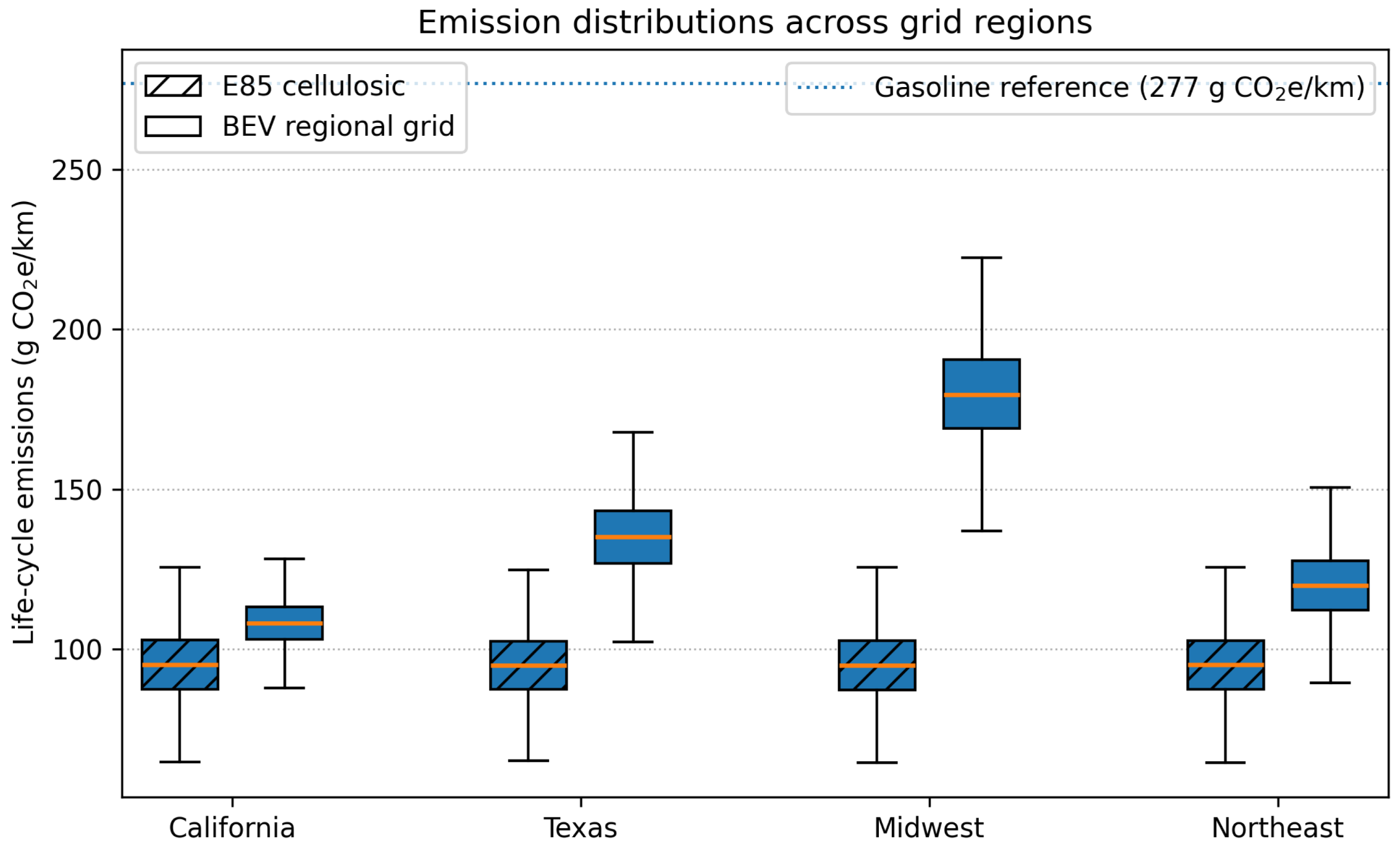
Figure 1 summarizes the multi-zone sensitivity framing for cellulosic E85 and BEV emissions. Cellulosic E85 exhibits regional stability because its dominant emissions arise from feedstock, conversion, and vehicle operation rather than grid carbon intensity. BEV emissions vary strongly by region: CAISO-zone BEVs overlap with cellulosic E85 under the stated scenario inputs, while MISO-MROW-zone BEVs remain substantially higher due to elevated grid carbon intensity.

4.5. PHEV Emission Reductions: CAISO Run and Extension Sensitivity Cases

Table 8. PHEV emission changes for AES relative to the static baseline, separated by evidence status.

Grid Zone	Static Baseline (g CO2e/km)	AES Optimized (g CO2e/km)	Mean Change (%)	Evidence Status
CAISO	181.76	123.38	32.12	Implemented CAISO/CAISO_NORTH proof-of-method run; 168/168 AES selections were cellulosic E85
ERCOT	165	119	28	Hypothetical extension sensitivity; not empirical
MISO-MROW	180	153	15	Hypothetical extension sensitivity; not empirical
ISO–NE	155	110	29	Hypothetical extension sensitivity; not empirical

Static baseline is defined in Section 3.3. Sensitivity values are useful for model exploration but should not be cited as completed regional empirical results until equivalent marginal-emissions, price, and service-event data are supplied.

separates the implemented CAISO result from prospective extension cases. In the CAISO case, the populated CSV audit reports that AES reduces PHEV emissions from 181.76 to 123.38 g CO₂e/km, a 32.12% reduction relative to the specified static baseline, with all 168 AES-selected events assigned to cellulosic E85. The ERCOT, MISO-MROW, and ISO–NE rows are not completed empirical dispatch results and should not be cited as regional reductions. They are retained only as hypothetical sensitivity outputs showing how the model would behave under declared extension-zone average factors and scenario inputs.

4.6. BEV-Only, PHEV, and E85-Only Comparison

Table 9. Comparative performance of BEV-only, PHEV with AES, and E85-only operation.

Grid Zone	BEV-Only Optimized (g CO2e/km, Mean ± Interval)	PHEV with AES (g CO2e/km)	E85-Only Cellulosic (g CO2e/km, Mean ± Interval)	Evidence Status
CAISO	Not supplied by current audit CSVs	123.38	123.38	Implemented PHEV proof-of-method; BEV-only requires separate output
ERCOT	$110\pm 20$	$119\pm 22$	$95\pm 22$	Hypothetical extension sensitivity
MISO-MROW	$168\pm 29$	$153\pm 24$	$95\pm 22$	Hypothetical extension sensitivity
ISO–NE	$98\pm 18$	$110\pm 20$	$95\pm 22$	Hypothetical extension sensitivity

Intervals denote propagated scenario uncertainty half-widths, not field-sampling confidence intervals. Extension-zone rows are hypothetical sensitivity outputs and are not completed empirical dispatch runs.

is retained as a pathway-comparison scaffold, but the populated CSV audit supplies only the implemented CAISO PHEV proof-of-method values. The uploaded files do not include a separate BEV-only optimized dispatch output; therefore the CAISO BEV-only entry is not populated from the present audit. The PHEV AES and E85-only CAISO entries coincide because the AES dynamic trace selected cellulosic E85 in all 168 events.

4.7. CAISO BEV–Cellulosic E85 Practical-Equivalence Result

The populated equivalence_tests.csv output does not support retaining the previous BEV–cellulosic E85 equivalence statement. For the supplied PHEV_FFV_CAISO pathway comparison, the mean difference for E85_cellulosic minus electric_annual_average is 28.48 g CO₂e/km with a 90% interval of 28.23–28.73 g CO₂e/km, and the test reports equivalent=False for the $\pm 10$ g CO₂e/km margin. Thus, the current archive supports only a narrower statement: annual-average electric operation is lower than the cellulosic E85 pathway under this PHEV pathway boundary, whereas the AES dynamic dispatch selected E85 in all events because the time-indexed marginal grid intensity during the audited week made electric operation less favorable in the carbon-priority objective. A separate BEV-only optimized output is required before making a BEV–E85 equivalence claim.

4.8. Battery-Production Amortization Sensitivity

Battery-production terms materially affect cross-technology comparisons. Using the declared battery-production intensity range in Table 6 and a 240,000 km lifetime, a 75 kWh BEV battery contributes 15.6–31.3 g CO₂e/km (central value 23.4 g CO₂e/km at 75 kg CO₂e/kWh), whereas a 14 kWh PHEV battery contributes 2.9–5.8 g CO₂e/km (central value 4.4 g CO₂e/km).

Table 10. Battery-production amortization sensitivity for declared battery capacities and lifetime.

Vehicle Battery Case	50 kg CO2e/kWh (g CO2e/km)	75 kg CO2e/kWh (g CO2e/km)	100 kg CO2e/kWh (g CO2e/km)
BEV, 75 kWh pack	15.6	23.4	31.3
PHEV, 14 kWh pack	2.9	4.4	5.8
Incremental BEV minus PHEV battery term	12.7	19.1	25.4

Values equal battery capacity multiplied by production intensity and divided by 240,000 km. They are not new empirical measurements; they expose the sensitivity already implied by the declared scenario parameters.

shows the arithmetic sensitivity implied by these declared parameters.

Because the populated CSV archive does not include a separate BEV-only optimized result, the previous numerical BEV–cellulosic E85 equivalence statement is not retained as an audited finding. Battery-production amortization remains important for any future BEV–PHEV–E85 comparison: adding the central incremental BEV-minus-PHEV battery term of 19.1 g CO₂e/km would materially change pathway rankings relative to a smaller-battery PHEV pathway comparison. Consequently, practical-equivalence statements are boundary-dependent and should be reported only when the corresponding BEV, PHEV, and liquid-fuel outputs are archived.

4.9. Example Daily Dispatch Profile

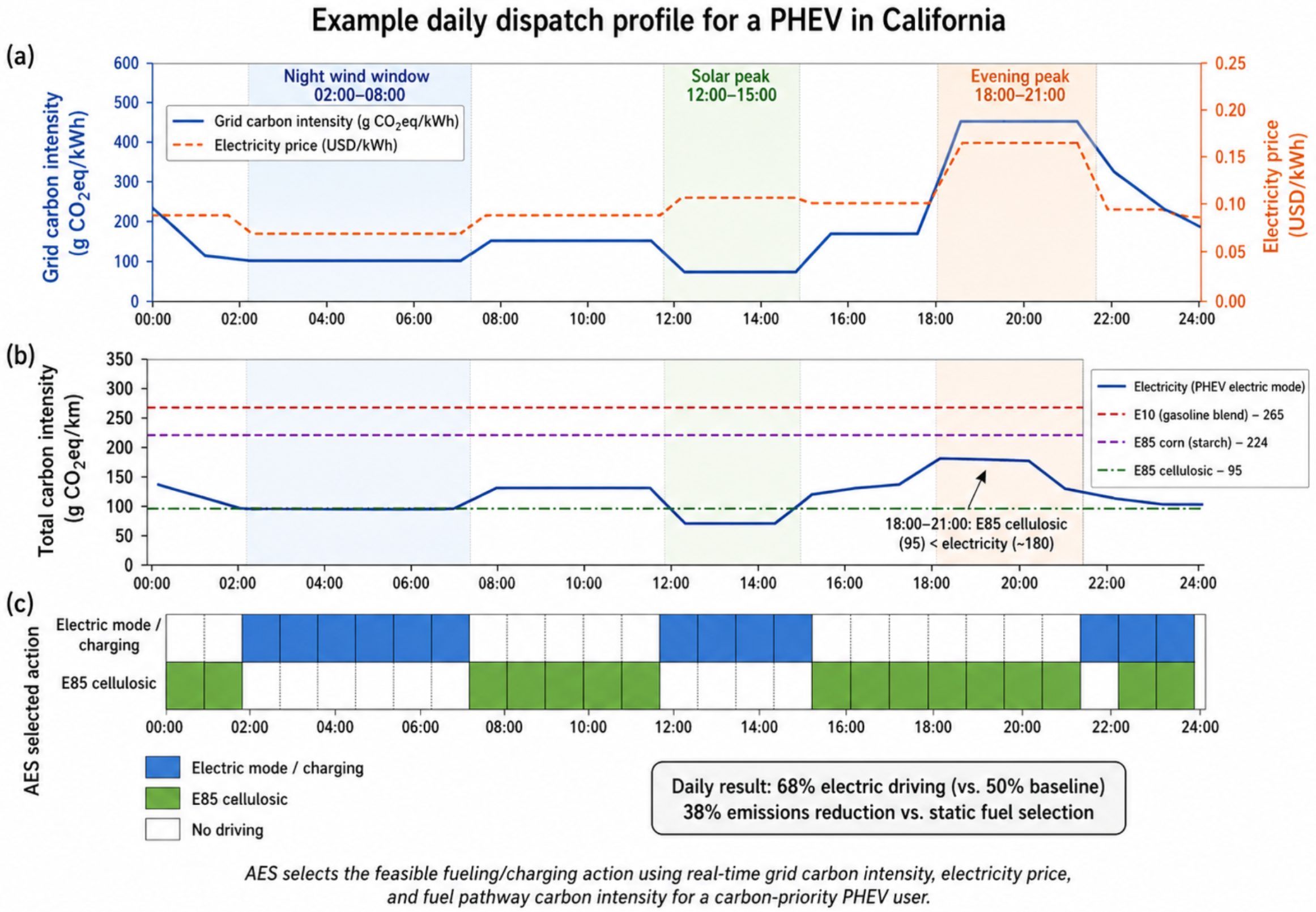
Figure 2 should be interpreted as a dispatch-profile diagnostic generated from the archived run inputs. In the populated CSV audit, however, the carbon-priority AES trace selects cellulosic E85 in all 168 service events and selects no electric charging events. The attached data therefore do not demonstrate within-week electric/E85 switching for this specific run; rather, they show that marginal grid carbon intensity remained high enough that cellulosic E85 was preferred whenever available and compatible.

5. Discussion

5.1. Operational Carbon Information Transforms Station-Level Decisions

Conventional LCA identifies promising technology pathways but cannot resolve the temporal windows during which electricity is substantially cleaner or dirtier than the annual average. The AES formulation bridges this gap by coupling pathway-level carbon-intensity factors with time-resolved marginal grid data and real-time vehicle constraints, enabling a station to generate transaction-level energy recommendations. The populated CAISO proof-of-method supports the narrower proposition that operational carbon information can alter transaction-level fuel choice relative to a static rule: the static baseline contains 85 electric and 83 E10 events, whereas the AES carbon-priority run selects cellulosic E85 in all 168 events. It does not, in this audited run, demonstrate electric/E85 temporal switching; that behavior remains a capability of the formulation to be tested in lower-MOER intervals, alternative fuel availability cases, or seasonal replications.

Compared with the recent vehicle-LCA literature, the CAISO AES result should be treated as complementary rather than contradictory. Studies by Verma et al. [6], Tang et al. [7], Kurkin et al. [8], Vieira et al. [9], Malik et al. [10], and Zajemska et al. [11] compare EV and fossil-fuel vehicle pathways across cradle-to-grave or well-to-wheel boundaries; they generally find that BEV results improve as electricity supply decarbonizes but remain sensitive to battery production, lifetime mileage, and regional grid mix. The present result instead reports a transaction-level PHEV station-dispatch outcome, so it should be compared to those studies as evidence that operational boundary and dispatch logic can change pathway selection, not as a replacement for full vehicle-platform LCA.

5.2. Regional Equivalence Is Conditional and Margin-Dependent

The populated equivalence-test output should be interpreted more narrowly than the earlier draft. It compares annual-average electric, E10, and cellulosic E85 pathway factors for the PHEV scenario, not a complete BEV-only optimized dispatch case. In that supplied file, E85_cellulosic exceeds electric_annual_average by 28.48 g CO₂e/km and is not equivalent at the $\pm 10$ g CO₂e/km margin. At the same time, the event-level AES dispatch selected E85 for all audited events because the marginal grid intensity during the selected winter week was high. This contrast reinforces the main methodological point: annual-average pathway comparisons and marginal-emissions dispatch decisions answer different questions. The extension cases illustrate conditionality only as hypothetical sensitivities; they are not evidence that the same reduction would occur in MISO-MROW, ERCOT, or ISO–NE without real marginal-emission and price data.

5.3. Temporal Optimization Benefits Are Region-Specific

The reported 32.12% emission reduction for the CAISO proof-of-method reflects the specific characteristics of one winter week and the declared service-event stream. It should not be interpreted as annual CAISO performance, as representative of summer or shoulder-season renewable patterns, or as a transferable regional reduction. The magnitude of temporal optimization benefits will differ in other regions depending on marginal-emission profiles, grid composition, price structures, and the flexibility of vehicle operators to shift charging times. This pattern is consistent with the broader smart-charging literature [2,3] and motivates seasonal replications before policy generalization.

5.4. PHEV Operational Flexibility and Its Limits

PHEVs are well suited to AES control because they expand the feasible action set beyond what is available to BEV-only or liquid-fuel-only vehicles. However, the results do not support characterizing PHEVs as universally superior. Their advantage is conditional resilience: the ability to use electricity when the grid is clean, switch to certified low-carbon liquid fuel when marginal emissions are elevated, and retain liquid-fuel range where charging infrastructure is limited. This flexibility depends on actual driver willingness to charge, charger access, dwell time, battery state, and verified fuel availability. As grids decarbonize and charging infrastructure matures, or if low-carbon liquid fuels are unavailable, the marginal value of PHEV flexibility may diminish—a trajectory that the AES framework can track through updated marginal-emission and availability inputs.

5.5. Policy Implications

The modeling results support technology-neutral, performance-based policies that reward verified carbon-intensity reductions rather than prescribing a single vehicle technology for all regions. Low-carbon fuel standards, clean electricity standards, smart-charging mandates, open marginal-emission data requirements, and station-level carbon reporting could all facilitate AES deployment. However, the policy interpretation is derived from regional and temporal variability in the model, not from a randomized policy trial. Public incentives should therefore be conditioned on measured carbon performance, infrastructure utilization, equitable user access, cybersecurity assurance, and verified supply-chain sustainability.

5.6. Limitations

Several limitations warrant acknowledgment. First, the executable implementation covers only one CAISO/CAISO_NORTH winter week (1–8 January 2026), which includes holiday-period operating conditions and should not be interpreted as seasonally or annually representative. We are investing our efforts in collecting, analysing, and formatting broader data available from US public agencies. A more robust assessment should incorporate stratified weeks or full-year runs covering seasonal variation, weekday/weekend effects, and high- versus low-renewable intervals, using public-agency sources such as EPA eGRID, EIA electricity and fuel data, CAISO OASIS market data, FHWA travel statistics, and NREL transportation-energy datasets where the variables match the AES input schema. Second, the reported implementation uses hourly service events; no separate 5 min station-control simulation is claimed. Third, user behavior is uncertain—drivers may ignore recommendations, prioritize travel time, refuse higher-cost lower-carbon options, or arrive with unexpected state-of-charge. The model represents user classes through fixed weights, but real behavior should be estimated from field trials. Fourth, infrastructure constraints are simplified: charger queues, feeder capacity, dispenser availability, E85 distribution, and station inventory can all constrain feasible dispatch. Queue penalties are inactive in the reported run and should be activated only when station-traffic data are available. Fifth, the cellulosic E85 pathway is a scenario option, not a claim of broad retail availability; deployment studies need supply constraints, certification, and station inventory data. Sixth, carbon-priority operation is the headline scenario, while a real station must consider cost, queueing, customer acceptance, and contractual constraints. Seventh, cybersecurity risks are material—AES depends on external data feeds, vehicle-to-infrastructure communication, and station controllers. Data spoofing or compromised carbon-intensity signals could produce incorrect recommendations; future deployments should include signed data streams, local fallback profiles, and anomaly detection. Eighth, infrastructure LCA and consequential market effects are excluded; large-scale AES deployment could affect electricity demand, ethanol markets, land use, and grid congestion, requiring consequential LCA and integrated energy-system modeling.

6. Conclusions

This study presents an AES framework for life-cycle-aware, time-resolved dispatch of electric charging and low-carbon liquid fuels at multi-fuel transport-energy stations. The main conclusions are:

• Static LCA is necessary but insufficient for station-level operational decisions because grid carbon intensity, prices, and feasible vehicle actions vary over time.
• In the CAISO/CAISO_NORTH proof-of-method case with 168 hourly service events over one winter week, 1–8 January 2026 Pacific time, AES-controlled PHEV operation reduces the reported scenario mean from 181.76 to 123.38 g CO₂e/km relative to the specified static baseline. This is not an annual CAISO result, not a fleet-adoption forecast, and not transferable without seasonal replication.
• ERCOT, MISO-MROW, and ISO–NE values are hypothetical extension sensitivity outputs, not completed empirical regional dispatch results; they should not be cited as measured regional reductions.
• The populated equivalence_tests.csv file does not support retaining the earlier BEV–cellulosic E85 equivalence claim as an audited result. It reports a PHEV-pathway comparison in which E85_cellulosic exceeds electric_annual_average by 28.48 g CO₂e/km and is not equivalent at the $\pm 10$ g CO₂e/km margin. A separate BEV-only optimized output is required before making a BEV–E85 equivalence claim.
• PHEVs should not be described as universally superior; their AES value is conditional operational flexibility across changing grid, price, infrastructure, driver-behavior, and certified fuel-supply conditions.

The policy conclusion is separate from the statistical results: AES can support performance-based, regionally flexible decarbonization policy only if data transparency, event-level dispatch auditing, infrastructure availability, cost sensitivity, user behavior, cybersecurity, and supply-chain sustainability are addressed.

References

1. Elgowainy, A.; Han, J.; Ward, J.; Joseck, F.; Gohlke, D.; Lindauer, A.; Ramsden, T.; Biddy, M.; Alexander, M.; Barnhart, S. Life-cycle analysis of greenhouse gas emissions from hydrogen delivery: A cost-guided analysis. Int. J. Hydrogen Energy 2018, 43, 16012–16024. [Google Scholar]
2. Graff Zivin, J.S.; Kotchen, M.J.; Mansur, E.T. Spatial and temporal heterogeneity of marginal emissions: Implications for electric cars and other electricity-shifting policies. J. Econ. Behav. Organ. 2014, 107, 248–268. [Google Scholar] [CrossRef] [Scilit]
3. Holland, S.P.; Mansur, E.T.; Muller, N.Z.; Yates, A.J. Are there environmental benefits from driving electric vehicles? The importance of local factors. Am. Econ. Rev. 2016, 106, 3700–3729. [Google Scholar] [CrossRef] [Scilit]
4. Bernardes, M.A.S. Environmental impact optimization of bifuel vehicles in Brazil using life cycle assessment and fuel selection. Int. J. Life Cycle Assess. 2009, 14, 533–541. [Google Scholar]
5. Bieker, G. A Global Comparison of the Life-Cycle Greenhouse Gas Emissions of Combustion Engine and Electric Passenger Cars; International Council on Clean Transportation: Berlin, Germany, 2021; Available online: https://theicct.org/publication/a-global-comparison-of-the-life-cycle-greenhouse-gas-emissions-of-combustion-engine-and-electric-passenger-cars/ (accessed on 22 June 2026).
6. Verma, S.; Dwivedi, G.; Verma, P. Life cycle assessment of electric vehicles in comparison to combustion engine vehicles: A review. Mater. Today Proc. 2022, 49, 217–222. [Google Scholar] [CrossRef] [Scilit]
7. Tang, B.; Wu, Z.; Li, Y. Life cycle assessment of battery electric and internal combustion engine vehicles under different electricity scenarios. Atmosphere 2022, 13, 252. [Google Scholar] [CrossRef] [Scilit]
8. Kurkin, A.; Rudenko, A.; Markov, A. Comparative life cycle assessment of electric and internal combustion engine vehicles. Energies 2024, 17, 2747. [Google Scholar] [CrossRef] [Scilit]
9. Vieira, V.; Sousa, R.; Martins, J. Comparison of battery electrical vehicles and internal combustion engine vehicles–greenhouse gas emission life cycle assessment. Appl. Sci. 2025, 15, 3122. [Google Scholar] [CrossRef] [Scilit]
10. Malik, F.H.; Alsharif, M.; Khalid, A. Evaluating carbon emissions: A lifecycle comparison between electric and conventional vehicles. World Electr. Veh. J. 2025, 16, 287. [Google Scholar] [CrossRef] [Scilit]
11. Zajemska, M.; Poskart, P.; Zajemski, K. A narrative review of life cycle assessments of electric vehicles: Methodological challenges and global implications. Energies 2025, 18, 5704. [Google Scholar] [CrossRef] [Scilit]
12. Argonne National Laboratory. GREET Model and Documentation; Argonne National Laboratory: Lemont, IL, USA, 2023. Available online: https://greet.anl.gov/ (accessed on 22 June 2026).
13. Nimesh, V.; Kumari, R.; Soni, N.; Goswami, A.K.; Mahendra Reddy, V. Implication viability assessment of electric vehicles for different regions: An approach of life cycle assessment considering exergy analysis and battery degradation. Energy Convers. Manag. 2021, 237, 114104. [Google Scholar] [CrossRef] [Scilit]
14. Olindo, R.; Schmitt, N.; Vogtländer, J. Life cycle assessments on battery electric vehicles and electrolytic hydrogen: The need for calculation rules and better databases on electricity. Sustainability 2021, 13, 5250. [Google Scholar] [CrossRef] [Scilit]
15. Shafique, M.; Luo, X. Environmental life cycle assessment of battery electric vehicles from the current and future energy mix perspective. J. Environ. Manag. 2022, 303, 114050. [Google Scholar] [CrossRef] [Scilit]
16. Oluwalana, O.J.; Adewumi, A.; Afshari, M. A systematic review of life cycle assessment of electric vehicles studies: Goals, methodologies, results and uncertainties. Energies 2025, 18, 5867. [Google Scholar] [CrossRef] [Scilit]
17. Cappelli, A.; Gargiulo, C.; Mazzarella, L. A comparative life cycle assessment of an electric and internal combustion vehicle. Energies 2025, 18, 3698. [Google Scholar] [CrossRef] [Scilit]
18. Horesh, N.; Zhou, Y.; Quinn, J. Home charging for all: Techno-economic and life cycle assessment of multi-unit dwelling electric vehicle charging hubs. J. Clean. Prod. 2023, 383, 135551. [Google Scholar] [CrossRef] [Scilit]
19. Vilaça, M.; Santos, G.; Oliveira, M.S.A.; Coelho, M.C.; Correia, G.H.A. Life cycle assessment of shared and private use of automated and electric vehicles on interurban mobility. Appl. Energy 2022, 310, 118589. [Google Scholar] [CrossRef] [Scilit]
20. Oliveri, L.M.; Lupi, F.; Rizzo, C. Electrifying green logistics: A comparative life cycle assessment. Energies 2023, 16, 7688. [Google Scholar] [CrossRef] [Scilit]
21. Rovelli, D.; Cornago, S.; Scaglia, P.; Brondi, C.; Low, J.S.C.; Ramakrishna, S.; Dotelli, G. Quantification of non-linearities in the consequential life cycle assessment of the use phase of battery electric vehicles. Front. Sustain. 2021, 2, 631268. [Google Scholar] [CrossRef] [Scilit]
22. Joshi, A.; Sharma, R.; Baral, B. Comparative life cycle assessment of conventional combustion engine vehicle, battery electric vehicle and fuel cell electric vehicle in Nepal. J. Clean. Prod. 2022, 379, 134407. [Google Scholar] [CrossRef] [Scilit]
23. Shang, H.; Sun, Y.; Huang, D.; Meng, F. Life cycle assessment of atmospheric environmental impact on the large-scale promotion of electric vehicles in China. Resour. Environ. Sustain. 2024, 15, 100148. [Google Scholar] [CrossRef] [Scilit]
24. Liu, Y.; Liu, Q.; Gao, L.; Xing, Y.; Chen, Y.; Zhang, S. The life cycle assessment and scenario simulation prediction of intelligent electric vehicles. Energy Rep. 2024, 12, 6046–6071. [Google Scholar] [CrossRef] [Scilit]
25. Zheng, G.; Peng, Z. Life cycle assessment (LCA) of BEV’s environmental benefits for meeting the challenge of ICExit (internal combustion engine exit). Energy Rep. 2021, 7, 1203–1216. [Google Scholar] [CrossRef] [Scilit]
26. Miller, G.J.; Novan, K.; Jenn, A. Hourly accounting of carbon emissions from electricity consumption. Environ. Res. Lett. 2022, 17, 044073. [Google Scholar] [CrossRef] [Scilit]
27. WattTime. How Emissions-Optimized EV Charging Enables Cleaner Electric Vehicles; WattTime: Oakland, CA, USA, 2024; Available online: https://watttime.org/wp-content/uploads/2024/01/WattTime-EVAnalysis-FullReport-vFinal.pdf (accessed on 22 June 2026).
28. SAE J2841; Utility Factor Definitions for Plug-In Hybrid Electric Vehicles Using Travel Survey Data. SAE International: Warrendale, PA, USA, 2010.
29. Plötz, P.; Moll, C.; Li, Y.; Bieker, G.; Mock, P. Real-world usage of plug-in hybrid electric vehicles: Fuel consumption, electric driving, and CO2 emissions. Transp. Res. Part D Transp. Environ. 2020, 84, 102365. [Google Scholar] [CrossRef] [Scilit]
30. Duoba, M.; Pulpeiro González, J. Updating Utility Factor (UF) Calculations in SAE J2841: Analyzing Charging Behaviors and Other Real-World Impacts on PHEV UF. In Proceedings of the 38th International Electric Vehicle Symposium and Exhibition (EVS38), Göteborg, Sweden, 15–18 June 2025. [Google Scholar]
31. Wang, M.; Han, J.; Dunn, J.B.; Cai, H.; Elgowainy, A. Well-to-wheels energy use and greenhouse gas emissions of ethanol from corn, sugarcane and cellulosic biomass for US use. Environ. Res. Lett. 2012, 7, 045905. [Google Scholar] [CrossRef] [Scilit]
32. Lavrador, R.B.; Teles, B.A.S. Life cycle assessment of battery electric vehicles and internal combustion vehicles using sugarcane ethanol in Brazil: A critical review. Clean. Energy Syst. 2022, 2, 100008. [Google Scholar] [CrossRef] [Scilit]
33. Lai, X.; Chen, Q.; Tang, X.; Zhou, Y.; Gao, F.; Zheng, Y. Critical review of life cycle assessment of lithium-ion batteries for electric vehicles: A lifespan perspective. eTransportation 2022, 12, 100169. [Google Scholar] [CrossRef] [Scilit]
34. Xia, X.; Li, P. A review of the life cycle assessment of electric vehicles: Considering the influence of batteries. Sci. Total Environ. 2022, 814, 152870. [Google Scholar] [CrossRef] [Scilit] [PubMed]
35. Feng, T.; Guo, W.; Li, Q.; Meng, Z.; Liang, W. Life cycle assessment of lithium nickel cobalt manganese oxide batteries and lithium iron phosphate batteries for electric vehicles in China. J. Energy Storage 2022, 52, 104767. [Google Scholar] [CrossRef] [Scilit]
36. Chen, Q.; Lai, X.; Gu, H.; Tang, X.; Gao, F.; Han, X.; Zheng, Y. Investigating carbon footprint and carbon reduction potential using a cradle-to-cradle LCA approach on lithium-ion batteries for electric vehicles in China. J. Clean. Prod. 2022, 369, 133342. [Google Scholar] [CrossRef] [Scilit]
37. Wu, W.; Cong, N.; Zhang, X.; Yue, Q.; Zhang, M. Life cycle assessment and carbon reduction potential prediction of electric vehicles batteries. Sci. Total Environ. 2023, 903, 166620. [Google Scholar] [CrossRef] [Scilit] [PubMed]
38. Fan, T.; Liang, W.; Guo, W.; Feng, T.; Li, W. Life cycle assessment of electric vehicles’ lithium-ion batteries reused for energy storage. J. Energy Storage 2023, 71, 108126. [Google Scholar] [CrossRef] [Scilit]
39. Lavigne Philippot, M.; Costa, D.; Cardellini, G.; De Sutter, L.; Smekens, J.; Van Mierlo, J.; Messagie, M. Life cycle assessment of a lithium-ion battery with a silicon anode for electric vehicles. J. Energy Storage 2023, 60, 106635. [Google Scholar] [CrossRef] [Scilit]
40. Accardo, A.; Garofalo, A.; Dotelli, G.; Spessa, E. Prospective LCA of next-generation cells for electric vehicle applications. IEEE Access 2024, 12, 19584–19597. [Google Scholar] [CrossRef] [Scilit]
41. Benveniste, G.; Sánchez, A.; Rallo, H.; Corchero, C.; Amante, B. Comparative life cycle assessment of Li-sulphur and Li-ion batteries for electric vehicles. Resour. Conserv. Recycl. Adv. 2022, 15, 200086. [Google Scholar] [CrossRef] [Scilit]
42. Yang, H.; Hu, X.; Zhang, G.; Dou, B.; Cui, G.; Yang, Q.; Yan, X. Life cycle assessment of secondary use and physical recycling of lithium-ion batteries retired from electric vehicles in China. Waste Manag. 2024, 178, 168–175. [Google Scholar] [CrossRef] [Scilit] [PubMed]
43. Scrucca, F.; Presciutti, A.; Baldinelli, G.; Barberio, G.; Postrioti, L.; Karaca, C. Life cycle assessment of Li-ion batteries for electric vehicles: A review focused on the production phase impact. J. Power Sources 2025, 639, 236703. [Google Scholar] [CrossRef] [Scilit]
44. Degen, F.; Mitterfellner, M.; Kampker, A. Comparative life cycle assessment of lithium-ion, sodium-ion, and solid-state battery cells for electric vehicles. J. Ind. Ecol. 2025, 29, 113–128. [Google Scholar]
45. Ankathi, S.K.; Bouchard, J.; He, X. Beyond tailpipe emissions: Life cycle assessment unravels battery’s carbon footprint in electric vehicles. World Electr. Veh. J. 2024, 15, 245. [Google Scholar] [CrossRef] [Scilit]
46. Ahmadzadeh, O.; Rodriguez, R.; Getz, J.; Panneerselvam, S.; Soudbakhsh, D. The impact of lightweighting and battery technologies on the sustainability of electric vehicles: A comprehensive life cycle assessment. Environ. Impact Assess. Rev. 2025, 110, 107668. [Google Scholar] [CrossRef] [Scilit]
47. De Sio, P.; Gaito, M.; Esperto, V.; Cozzolino, E.; Astarita, A.; Tucci, F. Life cycle assessment of a composite prototype battery enclosure for electric vehicles. Sustainability 2025, 17, 1579. [Google Scholar] [CrossRef] [Scilit]
48. Shet, K.H.N.; Moholkar, V.S. Comparative life cycle analysis of hydrogen fuel cell electric vehicles and battery electric vehicles: An Indian perspective. Int. J. Hydrogen Energy 2025, 103, 729–739. [Google Scholar] [CrossRef] [Scilit]
49. ISO 14040:2006; Environmental Management—Life Cycle Assessment—Principles and Framework. ISO: Geneva, Switzerland, 2006.
50. ISO 14044:2006; Environmental Management—Life Cycle Assessment—Requirements and Guidelines. ISO: Geneva, Switzerland, 2006.
51. U.S. Environmental Protection Agency. Emissions & Generation Resource Integrated Database (eGRID), 2023 Data Release; EPA: Washington, DC, USA, 2025. Available online: https://www.epa.gov/egrid (accessed on 22 June 2026).