


Abstract
Sustainable hydrogen production in water-scarce regions poses critical environmental challenges due to limited freshwater availability and the energy intensity of seawater treatment. This study examines the environmental trade-offs of providing water for hydrogen production via seawater desalination (with or without brine treatment) or freshwater purification, using a comprehensive life cycle assessment (LCA) framework. The assessment centers on three water-stressed countries: the United Arab Emirates (UAE), Spain, and Australia. Results reveal clear trade-offs between freshwater conservation and marine environmental pressures. Brine treatment reduces nutrient-related marine impacts but increases energy-related burdens, particularly under fossil-dominated electricity systems. Water sourcing for electrolysis coupled with energy-intensive desalination systems generally exhibits higher environmental pressures than alternative configurations, whereas freshwater-based supply for hydrogen production pathways shows lower burdens in several impact categories but raise concerns regarding freshwater resource use. Sensitivity analysis confirms that system performance is strongly influenced by water demand and electricity characteristics, highlighting the importance of aligning hydrogen deployment strategies with regional energy and water conditions. Overall, the findings demonstrate that water sourcing decisions play a critical role in shaping the environmental sustainability of hydrogen systems in water-stressed regions and must be evaluated through integrated water–energy planning.
1. Introduction
The global shift toward decarbonization has placed hydrogen at the center of clean energy transitions, offering a pathway to reduce emissions in hard-to-abate sectors such as steelmaking, long-distance transportation, and energy storage [1,2]. While hydrogen itself produces no Greenhouse Gas (GHG) emissions at the point of use, its upstream production can be resource- and emission-intensive, particularly when considering electricity and water demands. As hydrogen deployment scales, growing concerns have emerged regarding the environmental trade-offs associated with its production, especially in regions already facing water stress [3,4].
Electrolysis, a process that splits water into hydrogen and oxygen using electricity, is increasingly favored as a green hydrogen pathway and is powered by renewable sources like wind and solar [5]. However, producing one kilogram of hydrogen via electrolysis requires approximately 9–18 kg of ultrapure water, depending on system design and operational losses [6,7,8]. In arid and semi-arid regions, this water demand is expected to be met through seawater desalination. Desalination, while expanding non-traditional water supply, imposes significant energy burdens and produces concentrated brine, which, if discharged untreated, can harm marine ecosystems [9,10]. Brine treatment (BT) technologies are often proposed to mitigate nutrient and salinity impacts, yet these systems require additional energy and materials that may exacerbate other environmental burdens [11].
Alternatively, hydrogen production through steam methane reforming (SMR) with or without carbon capture remains the dominant method globally. SMR has lower water purity requirements and typically exhibits lower electricity dependency than electrolysis but is associated with GHG emissions, and concerns over methane leakage [12,13].
Life cycle assessment (LCA) has become a key tool for evaluating the environmental performance of hydrogen systems. Numerous studies have compared hydrogen production methods in terms of global warming and energy consumption [14,15], while others have begun incorporating water consumption and freshwater scarcity metrics [16]. However, limited research has assessed the water sourcing impacts of desalination, brine discharge quality (e.g., nitrate content), and BT in hydrogen LCA studies. There is also a lack of regionalized assessments that account for country-specific electricity mixes and water supply strategies.
This study addresses these gaps by conducting a comparative LCA of 20 scenarios of water sourcing for hydrogen production across three water-stressed countries: Australia, the United Arab Emirates (UAE), and Spain. Each region is characterized by distinct water scarcity profiles, desalination practices, and electricity grid compositions, making them suitable test beds for assessing hydrogen sustainability under real-world constraints.
The novelty of this work lies in its combined treatment of brine discharge quality, regionalized water–energy systems, and detailed comparison across production technologies. The findings aim to support policymakers and industry stakeholders in identifying hydrogen production strategies that are both environmentally sound and compatible with the water security needs of vulnerable regions.
The remainder of this paper is structured as follows: Section 2 reviews previous literature on hydrogen production pathways, water sourcing strategies, brine treatment, and the role of regional differences, highlighting gaps this study aims to address. Section 3 outlines the methodology, including the LCA model, scenario design, inventory parameters, and sensitivity analysis. Section 4 presents the results across midpoint and endpoint categories, including eutrophication, marine ecotoxicity, water consumption, and global warming potential. Section 5 discusses key findings, including trade-offs across regions, technologies, and water sourcing strategies, with a summary of policy implications. Section 6 concludes the study with future research directions and final reflections on regional hydrogen sustainability strategies.
2. Literature Review
Hydrogen production’s environmental sustainability has received significant attention, especially through LCA methodologies. While hydrogen is a clean energy carrier at the point of use, its upstream environmental impacts vary based on production methods, energy sources, and water inputs. Recent studies have expanded the understanding of these impacts, particularly concerning water sourcing and treatment in hydrogen production systems.
2.1. Hydrogen Production Pathways and Environmental Impacts
Electrolysis and SMR are prominent hydrogen production methods. Electrolysis, when powered by renewable energy, offers low GHG emissions but is electricity-intensive. Koj et al. [17] highlighted that the electricity demand of electrolysis technologies is the main contributor to environmental impacts and levelized costs in most considered cases. Conversely, SMR, especially when combined with carbon capture and storage, can achieve low GHG emissions if high capture rates and best practices are employed [18].
Recent studies like [19,20,21,22,23,24] have also examined the environmental impacts of hydrogen production methods. For instance, Gonzales-Calienes et al. [20] proposed a standardized LCA-based framework to quantify hydrogen production carbon intensity using consistent system boundaries, life cycle inventory development procedures, and data quality criteria. Their well-to-gate assessment compared multiple hydrogen technologies and demonstrated how harmonized methodological choices improve comparability across production pathways and support certification and regulatory frameworks. These developments highlight the growing importance of transparent LCA modeling structures when assessing hydrogen sustainability across different technological and geographic contexts, particularly when results are intended to inform policy thresholds or certification schemes.
Zhang et al. [21] performed a comparative LCA of hydrogen production via water electrolysis using onshore and offshore wind power, showing that offshore wind-based systems had slightly higher environmental impacts due to greater infrastructure requirements. However, their analysis did not examine water-related impact categories.
While previous works have broadly compared hydrogen production methods, this study deepens the analysis by explicitly modeling water sourcing for both production routes in combination with varying water sourcing strategies across three water-stressed countries. This enhances the understanding of how production technology interacts with local resource conditions, an area less explored in earlier comparative LCAs.
2.2. Water Sourcing and Desalination in Hydrogen Production
Water is a critical input for electrolysis. In regions with limited freshwater, seawater desalination becomes a practical option. However, desalination processes, particularly reverse osmosis (RO), are energy-intensive and produce brine, which poses environmental challenges [25,26]. Studies have assessed the life cycle environmental impact of seawater reverse osmosis (SWRO) desalination for potable and industrial water production. Additionally, integrating desalination with hydrogen production systems has been explored to address water and clean energy demands. Gude [27] outlined key sustainability challenges associated with desalination, including its high energy demand, brine discharge without adequate environmental impact consideration, and the absence of integrated assessments when desalination is used in emerging applications like hydrogen production. These limitations are particularly relevant in water-stressed countries aiming to scale up clean hydrogen.
Jijakli et al. [28] conducted a life cycle assessment of solar-powered desalination systems, evaluating their environmental impacts across various configurations and energy scenarios. While their study highlights the environmental trade-offs of solar desalination, it does not integrate hydrogen production or assess water feedstock implications within hydrogen LCAs. It is a similar gap in other studies like [29,30].
Vazquez-Sanchez et al. [31] performed an LCA of PEM electrolysis integrated with seawater desalination in Saudi Arabia, finding that desalinated water had minimal contribution to total environmental impacts. The study is one of the first to incorporate the contribution of desalination impacts to hydrogen production LCA. However, the study used midpoint-only indicators and did not include brine composition or endpoint impact analysis. It also focused only on hydrogen production by electrolysis. This study advances that scope by incorporating brine treatment and endpoint categories, offering deeper insight into water-related trade-offs in hydrogen systems. This study also includes SMR in addition to electrolysis, as well as impacts of different regions’ electricity mix impacts on the studied indicators.
This study bridges that gap by assessing the impact of using desalinated water as a feedstock for both SMR and electrolysis, factoring in local desalination energy intensities. Unlike previous analyses, it also includes BT energy loads and evaluates scenarios with and without BT integration, making the environmental trade-offs more transparent for policymakers.
2.3. Brine Management and Environmental Concerns
Brine discharge from desalination plants can lead to marine environmental issues [32]. Different brine management methods have been reviewed by Ahmed et al. [33], with a focus on reducing environmental issues associated with brine disposal.
Unlike most hydrogen-related LCA studies that ignore or simplify brine discharge assumptions, this study quantifies the environmental consequences of brine composition, especially nitrate concentration, and integrates the effects of BT into LCA midpoint and endpoint categories. By doing so, it provides a novel attempt to assess the lifecycle trade-offs of integrating BT into hydrogen production from an environmental perspective. The specific technologies and processes included under the BT are detailed in Section 3.3, where their integration into this LCA framework is also explained.
2.4. Sensitivity and Uncertainty Analyses in Hydrogen and Desalination LCAs
Sensitivity and uncertainty analyses are pivotal in enhancing the robustness and credibility of LCAs, especially for emerging technologies like hydrogen production and seawater desalination. These analyses help identify critical parameters influencing environmental impacts and assess the reliability of LCA outcomes under varying assumptions.
In the context of hydrogen production, several studies have underscored the importance of sensitivity analyses. For instance, a comprehensive review by Barahmand and Eikeland [34] highlighted that a significant proportion of LCA studies lack thorough uncertainty analyses, potentially compromising the reliability of their conclusions. Similarly, Cloete et al. [35] conducted a life-cycle inventory analysis of hydrogen and ammonia power generation, emphasizing the need for uncertainty quantification to capture the variability in environmental impacts.
Desalination processes, particularly SWRO, have also been the subject of sensitivity analyses to determine the influence of operational parameters on environmental performance. Fayyaz et al. [36] demonstrated that a 10% reduction in electricity consumption in SWRO systems could lead to a 5% decrease in global warming and fossil resource depletion. A study by Najjar et al. [37] models multiple scenarios with varying electricity composition percentages for SWRO, but it does not conduct a formal sensitivity or uncertainty analysis.
Hybrid desalination systems have been evaluated for their environmental performance under varying operational conditions. Bordbar et al. [12] conducted sensitivity analyses on hybrid nanofiltration-desalination plants, finding that a ±20% variation in electricity input could result in substantial changes in impact categories such as climate change and human toxicity.
Furthermore, the integration of desalination with hydrogen production necessitates comprehensive sensitivity analyses to understand the compounded environmental effects. A study by Elgowainy et al. [38] expanded the greenhouse gases, Regulated Emissions, and Energy use in Transportation (GREET) model to include water consumption factors for hydrogen production pathways, highlighting the variability in water use based on production methods and energy sources. This work emphasizes the need for detailed assessments of water-related impacts in hydrogen production LCAs.
In summary, incorporating sensitivity and uncertainty analyses in LCAs of hydrogen production and desalination systems is essential for identifying key environmental hotspots and ensuring the reliability of sustainability assessments. These analyses facilitate informed decision-making by highlighting the parameters that most significantly influence environmental outcomes.
This study expands the scope of LCA sensitivity analysis by implementing a structured one-at-a-time (OAT) sensitivity analysis across multiple technical parameters related to water recovery, energy use, and brine composition. It is one of the few to do so for combined hydrogen and desalination systems.
2.5. Regional Considerations and Water Resource Management
Regional factors significantly influence the environmental performance of hydrogen production. For instance, in arid regions, the water demand for green hydrogen production raises concerns. Studies have assessed the water requirements for hydrogen production, emphasizing the importance of sustainable water management practices. Furthermore, the integration of water management strategies in offshore Power-to-X platforms has been evaluated to address water and energy demands. A study by Lee et al. [39] evaluated the impact of large-scale hydrogen production on regional water stress, considering local water supply and demand. This study compares the regional implications between three regions based on the electricity mix differences.
Cabrera et al. [40] demonstrate how integrating desalination with wind energy and battery storage on Gran Canaria significantly reduced carbon emissions, by 77.4%, compared to grid-powered desalination. Their findings highlight the importance of decoupling desalination from fossil-dominated grids, a key conclusion echoed in this study, where electrolysis scenarios with desalinated water showed high global warming impacts. This alignment reinforces the relevance of region-specific electricity mixes in determining environmental performance across hydrogen and water systems.
2.6. Addressing the Literature Gaps
Table 1 highlights key characteristics and methodological choices across LCA studies related to hydrogen production, desalination, or their integration. It reveals that while most studies evaluated GWP, only a minority of studies included marine eutrophication, marine ecotoxicity, or water consumption indicators, despite their relevance in water-stressed or coastal regions. Electrolysis pathways received more attention than SMR, yet the type of electrolysis and the source of electricity (e.g., grid vs. renewables) were not always systematically compared.
Table 1.
Summary of Reviewed LCA Studies on Hydrogen and Desalination Pathways.
Sensitivity analysis was conducted in several studies to explore parameter uncertainties, but its depth and scope varied. Importantly, only a few studies assessed the impact of water feedstocks or explicitly modeled desalination systems for hydrogen production, and even fewer considered brine management, which is a critical environmental issue in seawater desalination. By addressing these gaps, particularly in terms of regional water feed integration, impact categories beyond GWP, and brine discharge, the present study offers a more comprehensive and policy-relevant LCA approach.
3. Methodology
3.1. Goal and Scope
The primary goal of this study is to evaluate the environmental consequences of feedwater for hydrogen production using different water sourcing and treatment strategies, particularly under the constraints of water scarcity. By applying LCA, the trade-offs between desalinated seawater, desalinated seawater with BT, and freshwater purification as water inputs for hydrogen production using either SMR or electrolysis are investigated. The analysis focuses on three water-stressed countries: Australia, the UAE, and Spain. These countries were selected based on their active involvement in hydrogen transition strategies and their regional variability in water availability, electricity generation mixes, and desalination practices [45,46,47]. This study also conducts a comprehensive sensitivity analysis across the 20 scenarios to evaluate parameter uncertainty.
3.2. Functional Unit and System Boundaries
The functional unit is defined as the production of 1 kg of hydrogen (H2) at the plant gate, irrespective of the production pathway or water source. This provides a consistent basis for comparing the environmental impacts of 20 scenarios across regions and production technologies.
The system boundary follows a cradle-to-gate approach, encompassing upstream raw material extraction, water treatment and purification, electricity generation, and excludes the hydrogen production processes via electrolysis or SMR themselves. Construction, maintenance, and end-of-life phases of desalination, brine treatment, and hydrogen production infrastructure are also excluded from the system boundary, with the analysis focusing on operational-phase impacts. Moreover, post-production activities, such as hydrogen compression, storage, distribution, or end-use combustion, are not included in the scope. In the present study, SMR scenarios are modeled without carbon capture and storage (CCS). Water recovery rates are based on representative literature values and are intended to reflect reasonable representative operating conditions rather than site-specific performance.
The analysis accounts for: energy requirements for water treatment (desalination, freshwater purification, and BT), water requirements for both electrolysis and SMR processes, brine discharge characteristics including nitrate concentration and heat content, and regional energy grid compositions to reflect local electricity emission factors in each country. Figure 1 shows the system boundary for this study.
Figure 1.
The study system boundary.
The scenario sets described in Table 2 were developed and assessed in this study, focusing on the environmental implications of different water sourcing strategies for hydrogen production. This structure enables consistent cross-comparison of the environmental performance of hydrogen production pathways under varying water sourcing and brine management strategies.
Table 2.
Study scenario sets description.
It should be noted that comparisons between electrolysis and steam methane reforming (SMR) in this study are limited to differences arising from water sourcing and treatment subsystems. Upstream fuel supply chains, hydrogen conversion efficiencies, carbon capture performance, and downstream hydrogen infrastructure are outside the comparative scope and are held constant or excluded to isolate the influence of water-related decisions in water-stressed regions.
3.3. Life Cycle Inventory (LCI) and Key Modeling Assumptions
The LCI was developed using secondary data sources to quantify water, energy, and material requirements associated with hydrogen water supply pathways. Inventory parameters and modeling assumptions were selected based on peer-reviewed literature and established databases to ensure consistency across scenarios.
Key model parameters, including process energy consumption, recovery rates, brine composition, and electricity supply characteristics, are summarized in Table 3. These parameters define the baseline system configuration used in the comparative assessment.
Table 3.
Key model assumptions and supporting data sources used in the LCA model.
A detailed description of data sources, parameter selection rationale, and supporting modeling assumptions is provided in Appendix F to ensure transparency of the inventory development process.
3.4. Life Cycle Impact Assessment (LCIA)
Impact assessment was conducted using the ReCiPe 2016 (v1.09), individualist perspective methodology at both the midpoint (problem-oriented) and endpoint (damage-oriented) levels. The midpoint categories considered in this study include global warming, marine eutrophication, marine ecotoxicity, and water consumption. Endpoint indicators include human health (DALYs), ecosystem quality (species·yr), and resource depletion cost (USD 2013). The midpoint and endpoint units are explained in Table 4 and Table 5, respectively.
Table 4.
Midpoint indicators units.
Table 5.
Endpoint indicators units.
Both Impact World+ and ReCiPe 2016 were applied during preliminary stages to ensure methodological robustness. The comparative results revealed no significant differences in the overall ranking or magnitude of key environmental impacts across scenarios. Based on this consistency and the broader interpretability of results in ReCiPe 2016, the current study reports findings using ReCiPe 2016 exclusively. This approach ensures methodological continuity while enabling more direct comparison with existing literature and greater insight into long-term damage categories.
All impact calculations were performed using SimaPro software version 9.6.0.1 PhD, and results were generated separately for each scenario using normalized and unnormalized values for clarity. Sensitivity impacts were evaluated using both absolute and percentage change metrics.
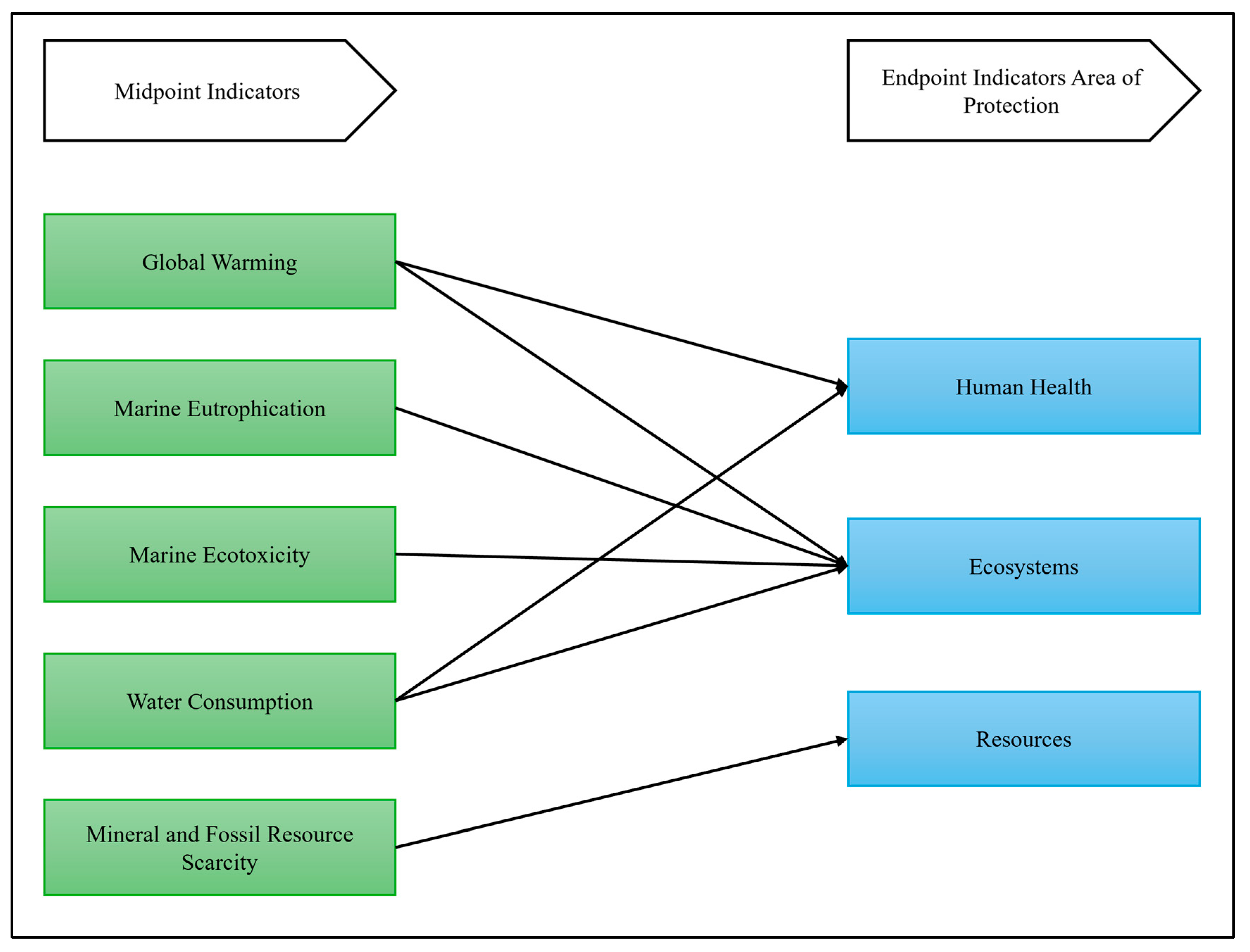
Endpoint indicators in ReCiPe 2016 represent aggregated global damage categories and do not explicitly resolve site-specific ecological impacts. Although ‘mineral and fossil resource scarcity’ is included for completeness, it was not a focus of the midpoint analysis in this study. The arrows represent causal pathways, where midpoint-level impacts contribute to damage at the endpoint level.
Marine ecotoxicity in the ReCiPe 2016 method is quantified using characterization factors expressed in 1,4-dichlorobenzene equivalents (kg 1,4-DCB eq), representing the relative toxic potential of emitted substances. Many major dissolved salts typically present in desalination brine do not have associated characterization factors for marine ecotoxicity within this method and therefore do not contribute to this impact category. Consequently, marine ecotoxicity results are primarily influenced by emissions from upstream processes, particularly energy production, where combustion-related emissions include substances characterized in terms of marine ecotoxicity potential.
Alternative water scarcity indicators, such as AWARE, could provide complementary insights; however, ReCiPe 2016 water consumption was selected to ensure consistency with endpoint damage modeling and comparability across midpoint and endpoint impact categories.
In ReCiPE 2016 framework [58], global warming contributes to two endpoint categories: human health (through heat stress and disease) and ecosystems (via climate-induced habitat shifts). Marine eutrophication and marine ecotoxicity primarily affect ecosystem quality [58]. This mapping helps translate technical emissions and resource use data into meaningful outcomes for decision-making and sustainability assessment. For reference, see Figure A2 in Appendix D for the relationship between the chosen midpoint impact categories and endpoint category indicators [58].
3.5. Sensitivity Analysis Design
This study developed 18 sensitivity iterations, each representing a variation in a single key assumption, as shown in Table 6. This allowed assessment of model responsiveness to changes in water demand, energy consumption, recovery efficiency, and nitrate discharge concentrations. This approach systematically varies individual parameters while holding all other inputs constant, allowing the relative importance of each parameter to be isolated and compared. The objective of this analysis is to identify dominant drivers of environmental impacts rather than to quantify overall system uncertainty.
Table 6.
Sensitivity Analysis assumed values for the iterations.
3.6. Sensitivity Analysis Equation
To quantify the effect of varying each parameter on the environmental outcomes, the relative change in each impact category was calculated using the following equation:
Here, the following applies:
- Is,it is the impact score of a given scenario under modified assumptions (i.e., during one of the 18 sensitivity iterations).
- Is,base is the corresponding impact score for the same scenario under baseline assumptions.
- In this equation, S denotes scenario, it denotes iteration, and base denotes baseline.
This formulation was applied to all midpoint and endpoint indicators in the ReCiPe 2016 framework. Positive values indicate an increase in environmental burden due to parameter change, while negative values indicate a reduction. The analysis allows for a direct comparison of model responsiveness across water sourcing, energy intensity, and brine discharge parameters.
Table 6 presents the baseline values, modified values, and the corresponding ranges reported in relevant literature. Each parameter was varied within the minimum, maximum, or average values found in peer-reviewed studies and industry reports to reflect realistic operational conditions. This approach strengthens the representativeness of the sensitivity analysis and ensures the scenarios tested are grounded in practical and regionally relevant evidence.
4. Results
4.1. Life Cycle Impact Assessment Results
This section presents the LCIA results for all 20 scenarios modeled in this study. The results are structured around ReCiPe 2016 midpoint and endpoint indicators and are used to assess the influence of hydrogen production pathway (electrolysis vs. SMR), water source (desalinated seawater, desalinated seawater with BT, and freshwater), and regional electricity mixes (Australia, UAE, and Spain). Absolute results for selected scenarios (scenarios with most impacted or highlighted results) are presented in Table 7 for midpoint and Table 8 for endpoint categories.
Table 7.
Midpoint indicator results.
Table 8.
Endpoint indicator results.
The absolute values for midpoint and endpoint results of all the scenarios are available in Table A1, Table A2, Table A3, Table A4, Table A5, Table A6, Table A7, Table A8, Table A9, Table A10, Table A11, Table A12, Table A13, Table A14, Table A15, Table A16, Table A17, Table A18, Table A19, Table A20, Table A21, Table A22, Table A23, Table A24, Table A25, Table A26, Table A27, Table A28, Table A29, Table A30, Table A31, Table A32, Table A33, Table A34, Table A35, Table A36, Table A37, Table A38, Table A39, Table A40, Table A41 and Table A42 in Appendix A. All comparative statements between electrolysis and SMR in this study are limited to water supply and treatment subsystems and should not be interpreted as overall hydrogen production sustainability rankings. Inclusion of full production processes and associated upstream and downstream impacts may result in different comparative outcomes.
4.1.1. Midpoint Indicator Results
The midpoint results reveal significant variation in environmental performance across scenarios, with electrolysis pathways generally showing higher burdens due to their electricity intensity inherited by the higher assumed water requirements compared with SMR. Four midpoint indicators were assessed: global warming, marine eutrophication, marine ecotoxicity, and water consumption.
In terms of global warming the highest impacts were observed in the water sourcing for electrolysis scenarios using desalinated water coupled with BT. The worst-performing case was Bii2-EL-AU, which recorded 0.323 kg CO2 eq/kg H2. On the other hand, the lowest global warming result was found in C2-SMR-AU at 0.0437 kg CO2 eq/kg H2.
The global warming values in this study reflect only the impact of water feed sourcing and treatment in the hydrogen production system. For context, full-process LCA studies such as [22] report total GWP values of 10.4 kg CO2-eq/kg H2 for SMR without CCS, 4.5 kg CO2-eq/kg H2 for SMR with CCS, and 2–3 kg CO2-eq/kg H2 for electrolysis powered by wind or solar energy. Although these figures are not directly comparable, they highlight that water feed can represent a meaningful share of life cycle climate impacts, particularly in water-stressed regions or systems requiring desalination. Thus, integrating water sourcing considerations is crucial for ensuring low-carbon hydrogen strategies.
Marine eutrophication was driven primarily by brine discharge characteristics and the presence of nitrates in the effluent. In scenarios without BT, such as A2-EL-AU, eutrophication levels were significantly higher due to direct discharge. A2-EL-AU exhibited the highest eutrophication value at 4.09 × 10⁻⁵ kg N eq. Freshwater-based water sourcing for the SMR scenario (C2-SMR-AU) had the lowest eutrophication impact, just 4.69 × 10⁻⁶ kg N eq, highlighting the importance of water source selection. Changes in marine eutrophication impacts across scenarios in this study arise from differences in nutrient emissions represented in the life cycle inventory rather than from an explicit nitrogen mass balance. The LCA software translates nutrient discharge, expressed as nitrogen-equivalent emissions, into marine eutrophication potential using characterization factors.
Notably, Bii5-SMR-AU, SMR with 100% BT, exhibited a higher global warming impact (0.161 kg CO2 eq/kg H2) and marine ecotoxicity (0.00273 kg 1,4-DCB) than all other SMR-based configurations, underscoring the indirect impacts of full treatment when powered by fossil-intensive grids.
Water consumption results were dominated by freshwater-based systems. C1-EL-AU recorded the highest water use at 11.10 m3/kg H2 due to the direct draw of freshwater resources. By contrast, desalination-based scenarios consumed less than 0.002 m3/kg H2 due to the LCIA assumption of seawater withdrawal not impacting water scarcity indicators. Among SMR systems, freshwater options (e.g., C2-SMR-AU) still showed relatively high consumption at 5.56 m3/kg H2. Although using freshwater as feedwater for SMR in Australia scenario (C2-SMR-AU) exhibited the lowest GWP among all scenarios, this benefit comes with a notable trade-off regarding water consumption impacts.
4.1.2. Endpoint Indicator Results
The endpoint assessment provided additional insight into the system-level damages associated with hydrogen production. Human health, ecosystem quality, and resource depletion costs were assessed using the ReCiPe 2016 endpoint framework. Absolute endpoint results are listed in Table 8 for selected scenarios.
Bii2-EL-AU again emerged as the most environmentally burdensome scenario. It recorded 1.30 × 10⁻⁷ DALY for human health, 7.25 × 10⁻¹⁰ species·yr for ecosystem damage, and 0.013924 USD 2013 for resource depletion. These values underscore the cumulative effect of energy-intensive water sourcing and fossil-based electricity, particularly in Australia.
In contrast, the best-performing scenario across all endpoint indicators was C2-SMR-AU. It had a human health impact of 2.20 × 10⁻⁸ DALY, ecosystem damage of 1.01 × 10⁻¹⁰ species·yr, and resource depletion cost of 0.00225 USD 2013. These outcomes demonstrate the potential of freshwater-based SMR, if water availability is not a limiting factor.
Scenarios employing BT consistently ranked higher in endpoint impacts than their non-BT counterparts. This finding supports the proposition that while BT reduces eutrophication, its energy and chemical intensity introduces greater burdens in other categories.
These results further emphasize the need to evaluate BT selectively by weighing the ecological benefits of nutrient reduction against the life cycle costs introduced by treatment energy demand.
4.2. Sensitivity Analysis Results
This section presents the results of the sensitivity analysis designed to evaluate the robustness of each scenario and identify the key drivers of environmental variability in hydrogen production systems. A total of 18 OAT iterations were applied to all scenarios by individually adjusting input parameters related to water demand, recovery efficiency, brine composition, and energy consumption for water treatment processes. Although the sensitivity analysis was conducted across all scenarios and regions, the results presented in this section focus on the Australian cases (AU) for clarity and brevity. The other regions, namely Spain and the UAE, exhibited similar trends in the direction and magnitude of change, reinforcing the generalizability of the findings. The results highlight how modest changes in model assumptions can drastically shift the environmental impacts in some of the iterations. The full sensitivity analysis results are presented in Table A43, Table A44, Table A45, Table A46, Table A47, Table A48, Table A49, Table A50, Table A51, Table A52, Table A53, Table A54, Table A55, Table A56, Table A57 and Table A58 in Appendix B.
4.2.1. Midpoint Sensitivity Results
The sensitivity analysis at the midpoint level revealed that water sourcing for electrolysis-based scenarios was significantly more sensitive to parameter changes than water sourcing for SMR-based systems. Among the various indicators, global warming and marine eutrophication showed the greatest responsiveness.
The largest increases in global warming impacts were observed in Iteration 2, where the water requirement for electrolysis was increased to 20 kg/kg H2. For instance, in Bii2-EL-AU, this resulted in a global warming impact increase of +122.2%. This sensitivity was mirrored in all midpoint impacts. For instance, marine eutrophication impacts rose sharply in iteration 2 (from 3.38 × 10⁻⁵ to 4.59 × 10⁻⁵ kg N eq). Marine ecotoxicity showed similar ranges of sensitivity to the results of global warming impacts for almost all iterations.
Conversely, Iteration 18, which modeled a higher nitrate concentration of 50 mg/L in brine (where baseline assumption was 10 mg/L), led to substantial differences in eutrophication impacts in BT scenarios. A2-EL-AU, an electrolysis scenario without BT, recorded a marine eutrophication increase of +195.4% under iteration 18, indicating that the absence of BT can exacerbate marine nutrient loading when water consumption increases. For Bi2-EL-AU (Australia with desalination and 20% BT), marine eutrophication increased in iteration 18 by +162.2% (absolute values from 3.95 × 10⁻⁵ kg N eq in the original scenario to 1.03 × 10⁻⁴ kg N eq after applying Iteration 18).
Water consumption was, as expected, most sensitive in freshwater-based systems. C1-EL-AU saw water consumption impact rise by 67% when electrolysis water requirements were increased in iteration 2 (from 11.1 m3 in baseline scenario to 18.5 m3 under iteration 2). On the other hand, desalination-based systems displayed relatively smaller midpoint impact result increases, as the water consumption impact parameter is not highly impacted if the water source is seawater.
Water sourcing for SMR scenarios (namely A5-SMR-AU, Bi5-SMR-AU, Bii5-SMR-AU, C2-SMR-AU), regardless of the water source, showed lower sensitivity in all midpoint indicators compared with water sourcing for electrolysis scenarios, with most values varying less than ±30%, showing their relative robustness under input uncertainty. The robustness may be attributed to the assumption that SMR requires half of the pure water amount that is required for electrolysis. Moreover, the iteration range for the water requirement for SMR is assumed to be from 4.5 to 5.8 kg water/kg H produced (Iteration 3 and Iteration 4). On the other hand, the iteration range for water requirement for electrolysis is from 9 to 20 kg water/kg H produced (Iteration 1 and Iteration 2). Hence, the results in Iteration 1 and Iteration 2 had much higher impacts on water sourcing for electrolysis scenarios compared to the impact of Iteration 3 and Iteration 4 on water sourcing for SMR scenarios. This means that comparing sensitivity analysis results for water sourcing for SMR against water sourcing for electrolysis would not provide significant implications. Nonetheless, changing parameters that impact both water sourcing for SMR and electrolysis (like recovery rates for desalination, specific energy consumption needed for seawater desalination, and so on) can yield a more meaningful implication comparing the robustness of SMR against electrolysis scenarios.
4.2.2. Endpoint Sensitivity Results
At the endpoint level, the same patterns were observed with greater system-wide implications. Bii2-EL-AU, the most environmentally intensive configuration, exhibited extreme sensitivity to water-related parameters. In Iteration 2, human health impacts, ecosystem damage, and resource depletion all rose by +122%
Again, Iteration 18 provided a contrasting effect. By assuming a higher nitrate load in brine, and modeling the effectiveness of BT, eutrophication impacts declined significantly, while endpoint indicators, particularly ecosystem impacts, slightly reduced after benefiting from improved discharge quality.
Water sourcing for SMR-based scenarios in Australia demonstrated relative stability across all endpoint categories. No iteration altered the human health, ecosystem, or resource depletion results by more than ±37%. The highest sensitivity result in water sourcing for the SMR scenario was observed in scenario Bii5-SMR-AU where Iteration 5 increased marine ecotoxicity by 37.1% compared to the baseline value. The other results for water sourcing for SMR in the Australia scenarios were sensitive by less than ±20%.
The results reveal substantial variability in environmental performance across scenarios, driven largely by energy mix, water source, and treatment strategy. To better understand the implications of these findings, the next section provides an in-depth discussion of the trade-offs identified, supported by sensitivity analysis and regional policy relevance.
5. Discussion
This section summarizes and discusses the main findings from the life cycle and sensitivity analyses, highlighting the key environmental trade-offs associated with different hydrogen production pathways, water sourcing methods, and regional contexts. It also reflects on the broader implications of the results for sustainable hydrogen deployment in water-stressed regions.
5.1. Interpreting the Trade-Offs Between Water Source and Production Method
This study has demonstrated that the environmental impacts of hydrogen production vary significantly depending on the water source, treatment strategy, energy context, and production method employed. The worst-performing configuration across all midpoint and endpoint categories was Bii2-EL-AU, which used desalinated seawater for electrolysis coupled with 100% BT in Australia.
In contrast, the best-performing configuration was C2-SMR-AU, representing water sourcing for SMR using freshwater in Australia. All water sourcing for SMR scenarios had almost half the impact values compared to their counterparts in water sourcing for Electrolysis scenarios, reflecting SMR feedwater’s lower energy intensity in water purification and reduced water requirements for SMR compared with electrolysis.
The results show a 634.1% increase in global warming impacts and 839.7% increase in marine ecotoxicity when comparing Bii2-EL-AU (water sourcing for electrolysis in Australia with desalination and full brine treatment) to C2-SMR-AU (water sourcing for SMR in Australia with freshwater purification), underlining the substantial environmental burden of electrolysis when powered by fossil-heavy grids and reliant on desalinated water with BT. In the UAE, the transition from no BT to full BT increased GWP by 75% in water sourcing for electrolysis scenarios (A1-EL-AE vs. Bii1-EL-AE). Conversely, eutrophication impacts were reduced by approximately 40%. This trend is similar for Australia scenarios. This confirms that while BT offers pollution mitigation, its energy burden must be managed through low-carbon grid integration.
Eutrophication in estuarine and coastal marine ecosystems is primarily driven by excess nutrient inputs (especially nitrogen compounds like nitrate) which stimulate the overproduction of marine phytoplankton and algae. This process can lead to a cascade of harmful outcomes, including harmful algal blooms (e.g., dinoflagellates) that are toxic or inedible to marine life, reductions in water clarity, and increased nuisance blooms of gelatinous zooplankton. Over time, it alters species composition, reducing biodiversity and favoring less desirable or invasive species. The death and decline of coral reef communities are also frequently linked to eutrophic conditions, along with elevated pH, oxygen depletion (hypoxia), and increased risk of mass fish kills. These effects not only disrupt ecosystem stability but also have socioeconomic implications through losses in fisheries, recreational value, and coastal aesthetics [59]. Therefore, even though the modeled per-kilogram values are low, the potential for local or regional harm remains a valid concern in high-density hydrogen infrastructure near coastal zones.
Marine ecotoxicity exhibited counterintuitive trends. Marine ecotoxicity results, expressed in 1,4-DCB equivalents, were highest in scenarios involving brine treatment. This impact is almost solely attributed to the energy consumption required for these processes. In particular, the combustion of fossil fuels for electricity generation contributed significantly to 1,4-DCB emissions upstream. This explains why scenarios with higher energy consumption exhibit increased marine ecotoxicity even when brine composition remains similar. Although marine ecotoxicity was included in the analysis to investigate potential toxic effects from direct brine discharge, the results indicate that energy-related emissions (not the brine discharge composition) are the dominant factor [58]. The negligible impact from brine discharge towards marine ecotoxicity indicators is based on literature that suggests negligible amounts of 1,4-dichlorobenzene (1,4-DCB) equivalents associated with brine characteristics [51,52,53,54,55,56]. However, marine ecotoxicity induced by brine discharge combined with energy consumption can result in these substances accumulating in aquatic food chains, impairing reproductive and developmental processes in marine life, and ultimately disrupting entire ecosystems by reducing biodiversity and altering species composition [58]. This highlights the importance of decarbonizing energy inputs for water treatment when targeting ecotoxicity reduction. Under future decarbonized electricity mixes, the environmental performance of energy-intensive processes such as desalination, brine treatment, and electrolysis would improve substantially. In such contexts, the trade-offs observed between climate-related impacts and marine eutrophication reduction would be partially alleviated, strengthening the environmental case for integrated desalination–electrolysis systems in regions with low-carbon power generation.
The freshwater-based water sourcing for electrolysis scenario (C1-EL-AU) recorded a water consumption impact of 11.1 m3/kg H2, over 7000 times greater than desalination-based scenarios, which consumed less than 0.002 m3/kg H2. This significant contrast is due to ReCiPe 2016’s assumption that seawater withdrawals exert negligible pressure on water scarcity. This highlights a key trade-off: freshwater sourcing for SMR and electrolysis can be efficient in emissions but extremely intensive in water consumption. Reliance on purified freshwater leads to elevated water consumption impacts, which relate to freshwater resource depletion and water scarcity concerns, particularly in regions already facing water stress. This underscores the importance of considering both climate and water-related impacts when evaluating hydrogen production strategies. The water consumption indicator primarily reflects depletion of freshwater resources and therefore assigns substantially lower burdens to seawater use, which is consistent with the characterization framework of ReCiPe 2016. However, this does not imply that seawater abstraction or desalination is environmentally benign, particularly in coastal regions experiencing marine ecological stress. In this study, environmental pressures associated with seawater use are captured through other impact pathways, including energy-related emissions, marine eutrophication, and marine ecotoxicity linked to desalination and brine discharge processes. Consequently, interpretation of water sourcing sustainability should consider the full set of impact indicators rather than water consumption alone, especially when evaluating trade-offs between freshwater conservation and marine environmental pressures.
Consequently, the relative performance observed between electrolysis- and SMR-based scenarios reflects differences in water-feed management rather than a full life cycle comparison of hydrogen production technologies. Comparing full pathway LCA results can result in different rankings as the total pathway impacts would be different.
Table 9 provides a qualitative comparison of regional factors (such as electricity grid composition, water source) that influence the environmental impacts of hydrogen production across the UAE, Australia, and Spain. It highlights how identical technologies can yield markedly different results depending on local conditions.
Table 9.
Qualitative Comparison of Regional Factors Influencing Hydrogen Environmental Impacts.
5.2. The Role of Regional Energy Mix and Infrastructure
The regional electricity grid composition had a dominant influence on hydrogen’s environmental performance. The Australian scenarios, due to the country’s coal-heavy energy mix, consistently ranked highest in all impact categories, and the UAE followed closely. Spain demonstrated better performance across the board, owing to its higher share of renewable electricity and lower energy demands for desalination. For instance, electrolysis using desalinated water in Australia (A2-EL-AU) emitted 0.181 kg CO2 eq/kg H2, while the same configuration in Spain (A3-EL-ES), which has higher renewable integration, emitted only 0.141 kg CO2 eq/kg H2, a 22% reduction.
Water sourcing for Electrolysis only offers meaningful climate benefits when coupled with low-carbon power. The sensitivity analysis confirmed this: under Iteration 2 (increased water requirement), global warming impact for Bii2-EL-AU increased by 122.2%, human health damage by 122.2%, and ecosystem damage by 121.9%. No comparable increase was observed in C2-SMR-AU, confirming the vulnerability of electrolysis systems to both water and electricity inputs.
It is important to note that electricity grid composition is a dynamic parameter; as the energy mix transitions toward renewables in the future, the environmental impacts associated with electrolysis are expected to decrease substantially.
These findings confirm that both water sourcing and regional energy context are critical to the environmental performance of hydrogen production pathways. Policy and infrastructure decisions should account for these contextual factors to ensure truly sustainable hydrogen deployment.
5.3. Insights from Sensitivity Analysis
The sensitivity analysis provided crucial insights into the most influential parameters driving environmental outcomes. Water sourcing for Electrolysis pathways was particularly sensitive to assumptions about water demand, BT efficiency, and energy intensity. For example, when ultrapure water demand for electrolysis was increased from 9 to 20 kg/kg H2 (Iteration 2), global warming rose by 122.2%, human health impacts increased by 122.2%, and resource depletion by 122.1% for Bii2-EL-AU.
Likewise, the marine eutrophication impact in A2-EL-AU (water sourcing for electrolysis without BT) increased by 195.4%, highlighting how nutrient loading from untreated brine scales with water usage. These impacts were also elevated due to Australia’s fossil-intensive electricity grid, exacerbating the trade-offs.
In contrast, scenarios assuming higher nitrate concentrations in brine (50 mg/L) and effective treatment systems (Iteration 18) reduced eutrophication impacts by 162.2% in Bi2-EL-AU, and lowered endpoint impacts by up to 37.1% in ecosystem damage, showing that well-implemented BT can offer important environmental co-benefits, though at an energy cost.
Marine ecotoxicity was also impacted by BT energy demand. For example, increasing the BT energy input from 10 to 15 kWh/m3 (Iteration 11) raised ecotoxicity by 14.3% in Bi2-EL-AU. Conversely, reducing freshwater purification energy to 0.1 kWh/m3 (Iteration 13) cut ecotoxicity by 8.2% in C1-EL-AU, showing the environmental benefit of high-efficiency water treatment.
Operational recovery rates in desalination and freshwater purification systems can vary due to feedwater composition, membrane performance, and operational management. The present study uses representative literature-based recovery values to maintain comparability across scenarios. While site-specific variability was not modeled explicitly, the sensitivity analysis explores the response of environmental outcomes to changes in recovery rate assumptions, thereby providing a structured assessment of how process performance variability may influence comparative results. For example, in the A2-EL-AU case, the recovery rate sensitivity iterations show that changing desalination recovery can materially shift results: Iteration 5 increases global warming and marine ecotoxicity by approximately +25.0% (25.03% and 25.05%, respectively) and increases marine eutrophication by +38.31%, whereas Iteration 6 reduces global warming and marine ecotoxicity by about −16.7% (−16.69% and −16.70%) and reduces marine eutrophication by −25.54%. Iteration 5 represents a lower desalination recovery rate (40%) and Iteration 6 represents a higher desalination recovery rate (60%), compared to the base assumption for desalination recovery rates (50%). These results indicate that recovery rate assumptions influence the magnitude of impacts (primarily through changes in energy intensity per unit water produced), while the comparative interpretation across scenarios remains guided by the broader water–energy configuration.
Water sourcing for SMR-based systems, such as C2-SMR-AU, demonstrated exceptional robustness. Across all 18 sensitivity iterations, none of the endpoint indicators fluctuated by more than ±20%, confirming the low sensitivity of SMR to input variation, primarily due to its low reliance on ultrapure water and stable fossil-based operation. This stability makes water sourcing for SMR a more predictable option in uncertain or resource-constrained contexts, even if its hydrogen production process GHG emissions profile is not negligible.
5.4. Implications for Policy and Planning in Water-Scarce Regions
The findings of this study carry several implications for sustainable hydrogen planning. In regions where fossil-based electricity and water stress intersect, water sourcing for electrolysis, particularly when combined with desalination and BT, may not be the most sustainable pathway. In these contexts, water sourcing for SMR, possibly paired with carbon capture along with the SMR process, can serve as an interim strategy while grid and water infrastructure evolve.
Grid decarbonization must proceed in parallel with hydrogen deployment to ensure that electrolysis can deliver environmental benefits. Even modest increases in renewable energy share can significantly reduce the emissions burden of water treatment and hydrogen generation. Governments should encourage co-located systems that integrate solar, wind, and hydrogen production, especially in regions with desalination infrastructure already in place.
BT strategies should be implemented appropriately and based on discharge regulations, ecological sensitivity, and electricity mix impacts on the environment. While BT reduces marine nutrient loading, it can increase global warming and resource depletion cost if not managed efficiently. Based on the sensitivity analysis, the contribution of brine discharge to marine eutrophication is highly dependent on its nitrate concentration. In regions where brine contains elevated nitrogen levels, untreated discharge poses a substantial risk to marine ecosystems by intensifying nutrient loading. Conversely, in cases where brine is low in nitrogen content, the environmental risk associated with direct discharge is significantly reduced, suggesting that under such conditions, controlled untreated release may be a more acceptable strategy.
The integration of brine reuse into hydrogen production presents a promising alternative that merits further exploration. Treated wastewater could reduce reliance on desalinated or freshwater sources while lowering marine discharge volumes. Although not modeled in this study, this pathway may offer a compelling blend of environmental and operational benefits.
To translate the study’s insights into actionable strategies, Table 10 presents key policy and investment recommendations. These are organized by theme and tailored to regional contexts, highlighting priorities such as grid decarbonization in the UAE and Australia, support for efficient desalination technologies, and selective use of brine treatment or CCS-SMR based on local conditions.
Table 10.
Policy and Investment Recommendations Based on LCA of Hydrogen Water Feed Strategies.
Although this study examines three water-stressed countries, the results should be interpreted as context-dependent rather than universally transferable. Environmental outcomes are strongly influenced by regional electricity mix, desalination characteristics, and local water sourcing assumptions. Consequently, the relative performance of water supply options may differ under alternative energy systems, treatment technologies, or site-specific operating conditions. The findings therefore provide insight into system-level trade-offs under the modeled conditions rather than general rankings applicable to all geographic settings.
This discussion has outlined the key environmental trade-offs of hydrogen production pathways in water-stressed regions, emphasizing the role of regional infrastructure, energy source, and brine management. To build on these insights, the next section offers concluding remarks and suggests avenues for future research to enhance the environmental sustainability of hydrogen deployment.
6. Future Research and Conclusions
Based on the study summary, recommendations are made for future research and policy direction, with the goal of supporting more environmentally resilient hydrogen strategies. The main conclusions of the study are then stated at the end of this section.
6.1. Limitations and Future Research Directions
This study is not without limitations. Brine composition was modeled using nitrate concentrations from literature and plant data, but site-specific variability may affect real-world outcomes. The study also excluded infrastructure impacts such as construction and decommissioning of desalination, BT, and hydrogen production facilities, which could be more relevant in long-term or smaller-scale systems. Although infrastructure-related impacts may be relevant in long-term or small-scale systems, their exclusion is consistent with comparative LCA studies emphasizing operational performance. Furthermore, the use of generic electricity mixes does not capture dynamic grid interactions, which could affect time-based emissions profiles, especially for systems integrating intermittent renewables.
The water consumption values used for hydrogen production represent theoretical (stoichiometric) requirements and do not explicitly include operational losses, cooling demand, purge streams, or plant-specific process configurations. Actual industrial water use may therefore be higher, particularly for electrolysis systems requiring high-purity feedwater. As a result, modeled water consumption likely reflects a lower-bound estimate of operational demand. While this assumption supports consistent comparison across scenarios and is partially explored through sensitivity analysis, detailed modeling of plant-level water balances was beyond the scope of this study.
The integration of CCS may influence overall environmental performance through additional energy demand and process modifications; however, its effect on water sourcing and treatment requirements is uncertain and was not evaluated in this study. Assessing the interaction between CCS deployment and water-related impacts represents a relevant direction for future research.
While this study integrates brine treatment in the life cycle perspective through nitrate concentration as a proxy for marine eutrophication, it does not account for the spatial variability of marine ecosystem sensitivity to brine discharge. Local factors such as water circulation, marine biodiversity hotspots, and proximity to coral reefs or seagrass beds can influence ecological outcomes considerably. Future studies should consider combining LCA with spatial risk modeling or marine impact frameworks such as species sensitivity distributions (SSDs) or marine impact indices to assess location-specific risks. However, in the absence of high-resolution spatial data across the three case regions, the nitrate-based midpoint was chosen to provide a generalizable yet conservative estimation of marine eutrophication-related impacts. Although this study uses nitrate concentration as a generalized proxy for brine impacts, it is important to acknowledge that local marine conditions significantly influence the environmental outcomes of brine discharge. Salinity is a primary physical stressor associated with desalination brine discharge. However, the ReCiPe 2016 impact assessment method does not provide characterization factors that directly represent ecological impacts from elevated salt concentrations. Consequently, this study represents potential environmental burdens from brine discharge using available proxy indicators, including marine eutrophication (primarily associated with nutrient loading such as nitrate) and marine ecotoxicity (associated with DCB emissions). These indicators provide partial representation of marine environmental pressures but do not explicitly quantify salinity-driven ecological effects.
Another key limitation of this study is the use of annual average electricity grid mixes, which may not fully capture the temporal dynamics of renewable energy generation, particularly in regions with high solar or wind variability. The use of country-level averages may mask sub-national heterogeneity; however, the objective of this study is to assess system-level trade-offs rather than site-specific outcomes. Moreover, incorporating temporally resolved electricity data could further refine results, particularly for electrolysis-based pathways, and represents a relevant avenue for future research. Electrolysis systems are highly sensitive to fluctuations in electricity source and availability, and the environmental performance of hydrogen production can vary significantly by hour or season. Incorporating time-resolved grid data or adopting a dynamic life cycle assessment (LCA) approach would provide a more accurate and granular understanding of these impacts. Future research should aim to model hourly or seasonal electricity profiles to better assess the real-world sustainability of electrolysis in different regional contexts, especially as countries decarbonize their grids.
Furthermore, because desalination, brine treatment, and hydrogen production are strongly coupled processes, interactions among parameters may influence system behaviour in ways not captured by one-at-a-time variation. Future work could extend this analysis through global or probabilistic sensitivity approaches to better capture parameter interactions in coupled water–energy–treatment systems.
Brine treatment was represented using a generic electrodialysis process with fixed energy consumption to ensure consistent comparison across scenarios. This simplified representation does not account for technology-specific performance, scalability, resource recovery, or salinity-dependent efficiency, and therefore introduces structural uncertainty, particularly when comparing different treatment extents.
Moreover, future research can consider the integration of alternative water sources such as treated wastewater or reclaimed industrial effluents, which may offer a viable means to reduce the environmental burdens associated with desalination and freshwater use. Incorporating temporal variability in electricity generation and water availability would enhance the accuracy (or robustness) of life cycle models, particularly in regions with seasonal fluctuations. Additionally, spatially explicit modeling of brine discharge and other hydrogen production processes’ localized ecological impacts could provide more accurate assessments of marine impacts. Local-scale ecological damages, like coastal environments, may require complementary site-specific assessment tools beyond the scope of this study. Finally, linking environmental life cycle results with techno-economic analysis and stakeholder perspectives would support more comprehensive and context-sensitive planning for hydrogen infrastructure.
6.2. Conclusions
This study has conducted a comprehensive LCA of feedwater for hydrogen production systems under varying water sourcing and treatment configurations, spanning 20 scenarios across three water-stressed countries: Australia, the UAE, and Spain. By combining detailed process inventories, regionalized energy mixes, and explicit modeling of brine discharge quality, the analysis offers new insights into the environmental trade-offs associated with hydrogen deployment in water-scarce contexts.
The results confirm that hydrogen production pathways vary widely in environmental performance depending on the water source, production method, and regional electricity characteristics. Water sourcing for Electrolysis using desalinated water with full BT in Australia (Bii2-EL-AU) was identified as the most environmentally intensive configuration, with a global warming of 0.323 kg CO2 eq/kg H2, human health impacts of 1.30 × 10⁻⁷ DALY, and ecosystem damage of 7.25 × 10⁻¹⁰ species·yr.
Brine discharge quality emerged as a critical factor influencing marine eutrophication impacts. The trade-off between marine protection and energy burden reinforces the need for selective BT, particularly in sensitive coastal areas.
The sensitivity analysis further demonstrated that water sourcing for electrolysis and SMR is highly susceptible to changes in water demand, energy input, and brine composition.
The regional electricity mix proved to be a dominant driver of environmental outcomes. The same water sourcing for the electrolysis system in Spain outperformed its counterparts in the UAE and Australia due to Spain’s higher share of renewable energy. These findings confirm that grid decarbonization is a prerequisite for realizing the environmental potential of green hydrogen, especially when paired with energy-intensive water treatment and sourcing strategies.
The results suggest that while electrolysis holds long-term promise, it may not be environmentally optimal in all contexts without parallel investments in clean electricity and efficient water systems. SMR, despite its association with fossil fuels, may serve as a viable transitional option in certain geographies.
These findings underscore the importance of aligning hydrogen production strategies with both energy and water sustainability goals. However, it is important to recognize that the environmental trade-offs identified in this study are dynamic. As electricity grids continue to decarbonize and more energy-efficient water treatment and brine management technologies become available, the relative burdens associated with different hydrogen pathways may shift significantly.
BT reduces marine eutrophication but increases energy demand, underlining the need for selective implementation. Regional factors, especially electricity mix and desalination technology, play a dominant role in shaping environmental outcomes. No single hydrogen strategy is optimal in all settings. Policymakers must tailor hydrogen pathways to local water, energy, and environmental conditions while investing in renewable energy, efficient water treatment, and appropriate levels of BT and reuse.
Hydrogen may be a promising solution for future energy systems, but it will only be sustainable if designed with water as a central consideration. This study offers guidance to ensure that the hydrogen transition supports, not undermines, climate and water security goals.
Author Contributions
H.A.A.-A.: Conceptualization, Methodology, Software, Validation, Formal analysis, Investigation, Resources, Data Curation, Writing—Original Draft, Writing—Review & Editing, Visualization, Funding acquisition. K.T.: Conceptualization, Validation, Resources, Writing—Review & Editing, Supervision, Project administration. All authors have read and agreed to the published version of the manuscript.
Funding
This research was funded by the United Arab Emirates Ministry of Higher Education and Scientific Research, grant number 202364044.
Data Availability Statement
The original contributions presented in this study are included in the article. Further inquiries can be directed at the corresponding authors.
Acknowledgments
This research was supported by the Watanabe Memorial Foundation for the Advancement of New Technology.
Conflicts of Interest
The authors declare no conflicts of interest.
Appendix A. Study Results for Midpoint and Endpoint Indicators
Table A1.
Midpoint impacts for Unit.
Table A2.
Midpoint impacts for A1-EL-AE.
Table A3.
Midpoint impacts for A2-EL-AU.
Table A4.
Midpoint impacts for A3-EL-ES.
Table A5.
Midpoint impacts for A4-SMR-AE.
Table A6.
Midpoint impacts for A5-SMR-AU.
Table A7.
Midpoint impacts for A6-SMR-ES.
Table A8.
Midpoint impacts for Bi1-EL-AE.
Table A9.
Midpoint impacts for Bi2-EL-AU.
Table A10.
Midpoint impacts for Bi3-EL-ES.
Table A11.
Midpoint impacts for Bi4-SMR-AE.
Table A12.
Midpoint impacts for Bi5-SMR-AU.
Table A13.
Midpoint impacts for Bi6-SMR-ES.
Table A14.
Midpoint impacts for Bii1-EL-AE.
Table A15.
Midpoint impacts for Bii2-EL-AU.
Table A16.
Midpoint impacts for Bii3-EL-ES.
Table A17.
Midpoint impacts for Bii4-SMR-AE.
Table A18.
Midpoint impacts for Bii5-SMR-AU.
Table A19.
Midpoint impacts for Bii6-SMR-ES.
Table A20.
Midpoint impacts for C1-EL-AU.
Table A21.
Midpoint impacts for C2-SMR-AU.
Table A22.
Endpoint impacts for Unit.
Table A23.
Endpoint impacts for A1-EL-AE.
Table A24.
Endpoint impacts for A2-EL-AU.
Table A25.
Endpoint impacts for A3-EL-ES.
Table A26.
Endpoint impacts for A4-SMR-AE.
Table A27.
Endpoint impacts for A5-SMR-AU.
Table A28.
Endpoint impacts for A6-SMR-ES.
Table A29.
Endpoint impacts for Bi1-EL-AE.
Table A30.
Endpoint impacts for Bi2-EL-AU.
Table A31.
Endpoint impacts for Bi3-EL-ES.
Table A32.
Endpoint impacts for Bi4-SMR-AE.
Table A33.
Endpoint impacts for Bi5-SMR-AU.
Table A34.
Endpoint impacts for Bi6-SMR-ES.
Table A35.
Endpoint impacts for Bii1-EL-AE.
Table A36.
Endpoint impacts for Bii2-EL-AU.
Table A37.
Endpoint impacts for Bii3-EL-ES.
Table A38.
Endpoint impacts for Bii4-SMR-AE.
Table A39.
Endpoint impacts for Bii5-SMR-AU.
Table A40.
Endpoint impacts for Bii6-SMR-ES.
Table A41.
Endpoint impacts for C1-EL-AU.
Table A42.
Endpoint impacts for C2-SMR-AU.
Appendix B. Sensitivity Analysis Results (Percentage Difference Values)
Table A43.
Sensitivity analysis for midpoint results for A2-EL-AU.
Table A44.
Sensitivity analysis for midpoint results for A5-SMR-AU.
Table A45.
Sensitivity analysis for midpoint results for Bi2-EL-AU.
Table A46.
Sensitivity analysis for midpoint results for Bi5-SMR-AU.
Table A47.
Sensitivity analysis for midpoint results for Bii2-EL-AU.
Table A48.
Sensitivity analysis for midpoint results for Bii5-SMR-AU.
Table A49.
Sensitivity analysis for midpoint results for C1-EL-AU.
Table A50.
Sensitivity analysis for midpoint results for C2-SMR-AU.
Table A51.
Sensitivity analysis for endpoint results for A2-EL-AU.
Table A52.
Sensitivity analysis for endpoint results for A5-SMR-AU.
Table A53.
Sensitivity analysis for endpoint results for Bi2-EL-AU.
Table A54.
Sensitivity analysis for endpoint results for Bi5-SMR-AU.
Table A55.
Sensitivity analysis for endpoint results for Bii2-EL-AU.
Table A56.
Sensitivity analysis for endpoint results for Bii5-SMR-AU.
Table A57.
Sensitivity analysis for endpoint results for C1-EL-AU.
Table A58.
Sensitivity analysis for endpoint results for C2-SMR-AU.
Appendix C. Electricity Mix Comparison Between the UAE, Australia and Spain
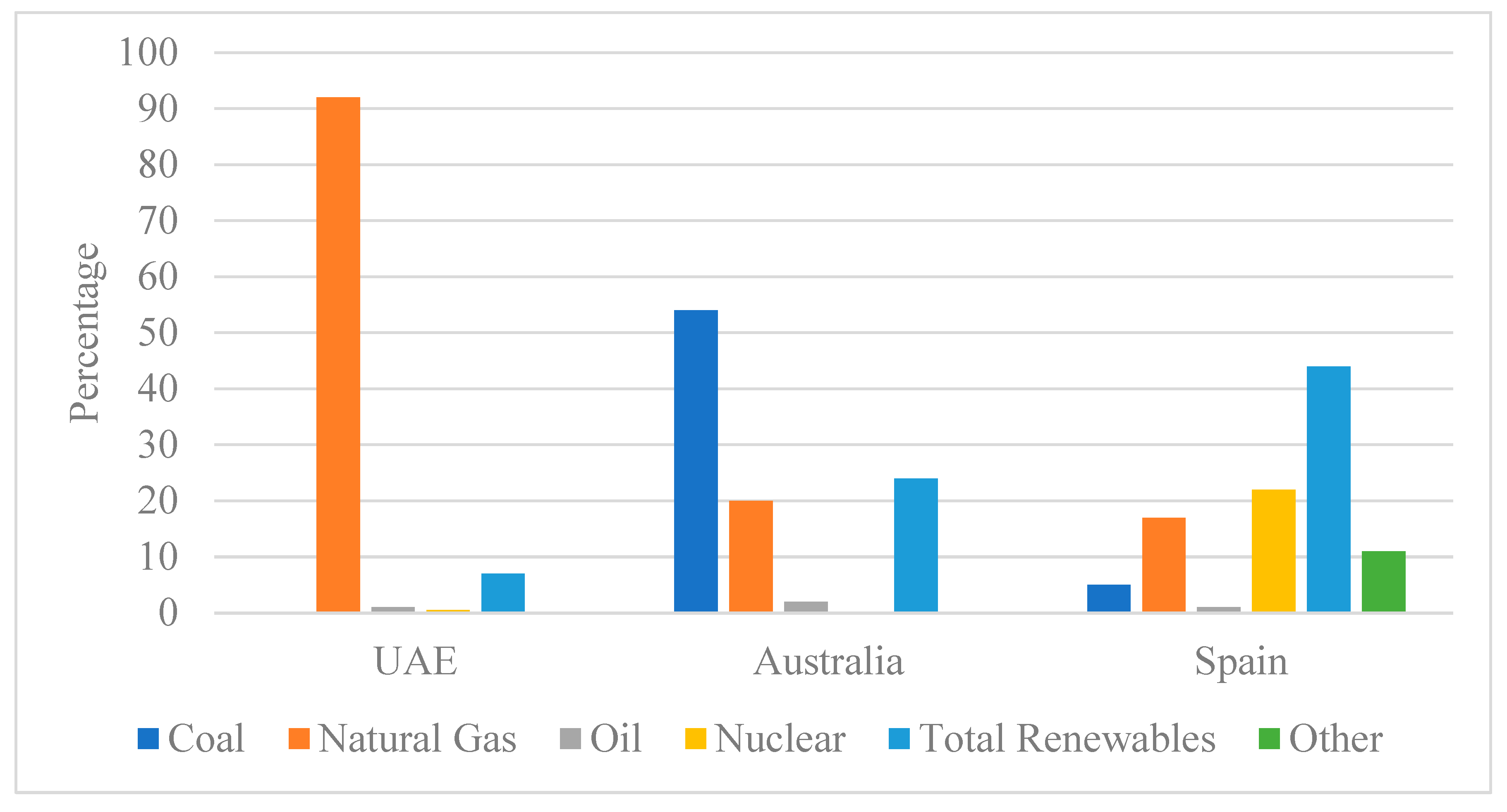
Figure A1.
Electricity mixes in the UAE, Australia and Spain [57].
Appendix D. Electricity Mix Comparison Between the UAE, Australia and Spain
Figure A2.
Relationship between Midpoint impact categories and endpoint category indicators [58].
Appendix E. Representative Brine Composition Used in LCA Inventory
Table A59.
Representative characteristics of major dissolved ions in desalination brine used in the study’s life cycle inventory, based on reported ranges for reverse osmosis discharge [51,52,53,54,55,56].
Appendix F. Supporting Documentation for LCI Parameterization
This appendix provides the detailed rationale and supporting documentation for the LCI parameters used in the modeling framework. To improve readability of the main methodological section, technical justification of parameter selection, data sources, and modeling choices is presented here. The information provided supports transparency, interpretability, and reproducibility of the inventory development process.
The LCI is built using secondary data sources. For hydrogen production, the inventory includes process-specific requirements for water, energy, and chemical inputs. For electrolysis, the baseline assumption is a requirement of 9 kg of ultrapure water per 1 kg of H2 produced. For SMR, the water demand is assumed to be 4.5 kg/kg H2. These values are based on the stoichiometric values of pure water requirements to simplify the assumptions [6,7].
Water purification processes include RO for seawater desalination, with an energy requirement of 3.5 kWh/m3 [48], and the sensitivity analysis considered the range 3.5–4.5 kWh/m3. Freshwater purification is modeled as requiring 1.0 kWh/m3 as average value [49], with sensitivity tested from 0.1 to 2.5 kWh/m3. BT is modeled at 10 kWh/m3 [49] under baseline assumptions, with sensitivity scenarios ranging from 7 to 15 kWh/m3. In this study, the term brine treatment (BT) refers to the additional treatment of desalination reject brine before discharge, in contrast to direct brine disposal into the marine environment. The assumed BT process is electrodialysis (ED/EDR), selected based on its technical feasibility in treating hypersaline waste streams. This assumption is informed by the findings of [50], who highlight the growing application of ED/EDR in Zero Liquid Discharge (ZLD) systems due to its ability to handle high salinity limits and recover valuable resources. The life cycle inventory for brine treatment incorporates additional energy and is associated with ED, reflecting its environmental impact within the LCA framework.
The recovery rate for seawater reverse osmosis (RO) desalination was assumed to be 50%, in line with values reported in [26], who provided a comprehensive review of energy consumption and operational performance of seawater desalination systems. The recovery rate for freshwater purification was assumed to be 81%, as supported by global assessments presented in [46] which highlight typical recovery rates for river water RO treatment processes.
Brine composition was modeled using empirically sourced nitrate concentrations to assess marine eutrophication and human health impacts. A baseline nitrate concentration of 10.7 mg/L was selected based on representative values reported in the literature, with sensitivity scenarios ranging from 0.01 to 50 mg/L to reflect possible variations observed in monitoring reports and field data. These values were drawn from published studies and discharge assessments in various desalination contexts [51,52,53,54,55,56].
Nitrate concentration in brine was modeled explicitly as a waterborne emission in the life cycle inventory, using the “Nitrate, ES” substance for Spain, “Nitrate, AU” for Australia and “Nitrate, AE” for the UAE. The assumed baseline value of 10.7 mg/L was multiplied by the total brine volume discharged to calculate the corresponding mass of nitrate released into the marine environment (e.g., 77.04 mg per functional unit in scenario Bi3-EL-ES). These emissions were assigned to the ocean sub-compartment and contributed to midpoint impact categories such as marine eutrophication as modeled by the fate and effect pathways in ReCiPe 2016. These impacts were further aggregated to endpoint indicators affecting ecosystem quality. The study does not perform an explicit mass balance of nitrogen species; instead, marine eutrophication impacts are calculated through characterization of nutrient emissions using established life cycle impact assessment factors. Variations in marine eutrophication results therefore reflect differences in modeled nutrient discharge associated with treated and untreated brine streams.
In addition to nitrate, other representative brine constituents were included in the model based on common brine discharge composition [52], such as sodium (Na+), calcium (Ca2+), chloride (Cl−), sulfate (SO42−), manganese compounds, and waste heat. The full list of assumed modeled concentrations is provided in Table A59 in Appendix E. While these substances were emitted to the same marine compartment, their contributions to midpoint and endpoint impact indicators were negligible compared to nitrate emissions. Therefore, nitrate was the dominant brine component influencing the marine-related environmental impacts modeled in this study.
Electricity consumption for all processes was aligned with national grid mixes, retrieved from the IEA and region-specific sources as used by the Ecoinvent database [54]. The electricity mix profiles are illustrated in Figure A1 in Appendix C, for reference. Electricity grid data for each country in the study (UAE, Spain, and Australia) was sourced from the Ecoinvent 3.9.1 database through SimaPro. We utilized low-voltage electricity market datasets of each country, which represent national-level consumption mixes. These datasets are modeled as market activities that account for production technologies, imports, grid transmission, and losses. National average electricity mixes were used to ensure consistency and comparability across the three case-study countries, recognizing that sub-national variability in grid composition and water scarcity may influence localized impact outcomes. Temporal variability in renewable generation is also not explicitly captured in this study.
For instance, the dataset “electricity, low voltage {AE}|market group|Alloc Def, U” reflects UAE’s national grid mix for the year 2020, based on IEA World Energy Statistics and Balances. It includes both domestic generation and imports, transmission network losses, and emissions associated with high-voltage transmission infrastructure [57].
Similar datasets were used for Australia and Spain, each representing the full national mix rather than regional sub-grids. As SimaPro’s spatial resolution is limited to country-level markets in these cases, finer spatial variations were not modeled. Nonetheless, the use of the most current country-level data ensures an accurate and consistent basis for comparative LCA across regions.
References
- International Energy Agency (IEA). Global Hydrogen Review 2021—Analysis—IEA. IEA. Available online: https://www.iea.org/reports/global-hydrogen-review-2021 (accessed on 5 March 2026).
- Buttler, A.; Spliethoff, H. Current status of water electrolysis for energy storage, grid balancing and sector coupling via power-to-gas and power-to-liquids: A review. Renew. Sustain. Energy Rev. 2017, 82, 2440–2454. [Google Scholar] [CrossRef] [Scilit]
- Ishaq, H.; Dincer, I.; Crawford, C. A review on hydrogen production and utilization: Challenges and opportunities. Int. J. Hydrogen Energy 2021, 47, 26238–26264. [Google Scholar] [CrossRef] [Scilit]
- Shahverdian, M.H.; Sohani, A.; Sayyaadi, H. A 3E water energy nexus based optimum design for a hybrid PV-PEMFC electricity production systems for off-gird applications. Energy Convers. Manag. 2022, 267, 115911. [Google Scholar] [CrossRef] [Scilit]
- Selvam, D.C.; Devarajan, Y.; Raja, T.; Vickram, S. Advancements in water electrolysis technologies and enhanced storage solutions for green hydrogen using renewable energy sources. Appl. Energy 2025, 390, 125849. [Google Scholar] [CrossRef] [Scilit]
- International Energy Agency (IEA). The Future of Hydrogen: Seizing Today’s Opportunities; IEA Publications: Paris, France, 2019; Available online: https://www.iea.org/reports/the-future-of-hydrogen (accessed on 5 March 2026).
- Nnabuife, S.G.; Darko, C.K.; Obiako, P.C.; Kuang, B.; Sun, X.; Jenkins, K. A comparative analysis of different hydrogen production methods and their environmental impact. Clean Technol. 2023, 5, 1344–1380. [Google Scholar] [CrossRef] [Scilit]
- International Renewable Energy Agency (IRENA) and Bluerisk. 2023 Water for Hydrogen Production. Available online: https://www.irena.org/Publications/2023/Dec/Water-for-hydrogen-production (accessed on 5 March 2026).
- Elimelech, M.; Phillip, W.A. The future of seawater desalination: Energy, technology, and the environment. Science 2011, 333, 712–717. [Google Scholar] [CrossRef] [Scilit]
- Gude, V.G.; Fthenakis, V. Energy efficiency and renewable energy utilization in desalination systems. Prog. Energy 2020, 2, 022003. [Google Scholar] [CrossRef] [Scilit]
- Panagopoulos, A.; Haralambous, K.-J. Environmental impacts of desalination and brine treatment—Challenges and mitigation measures. Mar. Pollut. Bull. 2020, 161, 111773. [Google Scholar] [CrossRef] [Scilit] [PubMed]
- Bordbar, B.; Khosravi, A.; Orkomi, A.A.; Peydayesh, M. Life cycle assessment of hybrid nanofiltration desalination plants in the Persian Gulf. Membranes 2022, 12, 467. [Google Scholar] [CrossRef] [Scilit] [PubMed]
- Voldsund, M.; Jordal, K.; Anantharaman, R. Hydrogen production with CO2 capture. Int. J. Hydrogen Energy 2016, 41, 4969–4992. [Google Scholar] [CrossRef] [Scilit]
- Bicer, Y.; Dincer, I.; Zamfirescu, C.; Vezina, G.; Raso, F. Comparative life cycle assessment of various ammonia production methods. J. Clean. Prod. 2016, 135, 1379–1395. [Google Scholar] [CrossRef] [Scilit]
- Aydin, M.I.; Dincer, I. A life cycle impact analysis of various hydrogen production methods for public transportation sector. Int. J. Hydrogen Energy 2022, 47, 39666–39677. [Google Scholar] [CrossRef] [Scilit]
- Mehmeti, A.; Angelis-Dimakis, A.; Arampatzis, G.; McPhail, S.; Ulgiati, S. Life cycle assessment and water footprint of hydrogen production methods: From conventional to emerging technologies. Environments 2018, 5, 24. [Google Scholar] [CrossRef] [Scilit]
- Koj, J.C.; Zapp, P.; Wieland, C.; Görner, K.; Kuckshinrichs, W. Life cycle environmental impacts and costs of water electrolysis technologies for green hydrogen production in the future. Energy Sustain. Soc. 2024, 14, 64. [Google Scholar] [CrossRef] [Scilit]
- Hydrogen Council 2021. Hydrogen Insights. 2021. Available online: https://hydrogencouncil.com/en/hydrogen-insights-2021/ (accessed on 5 March 2026).
- Martinez, G.E.; Degens, R.; Espadas-Aldana, G.; Costa, D.; Cardellini, G. Prospective Life cycle Assessment of Hydrogen: A Systematic Review of Methodological choices. Energies 2024, 17, 4297. [Google Scholar] [CrossRef] [Scilit]
- Gonzales-Calienes, G.; Kannangara, M.; Yang, J.; Shadbahr, J.; Bensebaa, F.; Alvarez-Majmutov, A.; Chen, J.; Mehr, N.G.; Benali, M. Life cycle assessment of hydrogen production pathways to support hydrogen decarbonization policies in a Canadian context. Front. Energy 2025, 19, 1093–1108. [Google Scholar] [CrossRef] [Scilit]
- Zhang, J.; Wang, Z.; He, Y.; Li, M.; Wang, X.; Wang, B.; Zhu, Y.; Cen, K. Comparison of onshore/offshore wind power hydrogen production through water electrolysis by life cycle assessment. Sustain. Energy Technol. Assess. 2023, 60, 103515. [Google Scholar] [CrossRef] [Scilit]
- Henriksen, M.S.; Matthews, H.S.; White, J.; Walsh, L.; Grol, E.; Jamieson, M.; Skone, T.J. Tradeoffs in life cycle water use and greenhouse gas emissions of hydrogen production pathways. Int. J. Hydrogen Energy 2023, 49, 1221–1234. [Google Scholar] [CrossRef] [Scilit]
- Zhang, J.; Ling, B.; He, Y.; Zhu, Y.; Wang, Z. Life cycle assessment of three types of hydrogen production methods using solar energy. Int. J. Hydrogen Energy 2022, 47, 14158–14168. [Google Scholar] [CrossRef] [Scilit]
- Osman, A.I.; Nasr, M.; Mohamed, A.R.; Abdelhaleem, A.; Ayati, A.; Farghali, M.; Al-Muhtaseb, A.H.; Al-Fatesh, A.S.; Rooney, D.W. Life cycle assessment of hydrogen production, storage, and utilization toward sustainability. WIREs Energy Environ. 2024, 13, e526. [Google Scholar] [CrossRef] [Scilit]
- Nassrullah, H.; Anis, S.F.; Hashaikeh, R.; Hilal, N. Energy for desalination: A state-of-the-art review. Desalination 2020, 491, 114569. [Google Scholar] [CrossRef] [Scilit]
- Kim, J.; Park, K.; Yang, D.R.; Hong, S. A comprehensive review of energy consumption of seawater reverse osmosis desalination plants. Appl. Energy 2019, 254, 113652. [Google Scholar] [CrossRef] [Scilit]
- Gude, V.G. Desalination and sustainability—An appraisal and current perspective. Water Res. 2015, 89, 87–106. [Google Scholar] [CrossRef] [Scilit]
- Jijakli, K.; Arafat, H.; Kennedy, S.; Mande, P.; Theeyattuparampil, V.V. How green solar desalination really is? Environmental assessment using life-cycle analysis (LCA) approach. Desalination 2011, 287, 123–131. [Google Scholar] [CrossRef] [Scilit]
- Raluy, R.G.; Serra, L.; Uche, J.; Valero, A. Life-cycle assessment of desalination technologies integrated with energy production systems. Desalination 2004, 167, 445–458. [Google Scholar] [CrossRef] [Scilit]
- Shahabi, M.P.; McHugh, A.; Anda, M.; Ho, G. Environmental life cycle assessment of seawater reverse osmosis desalination plant powered by renewable energy. Renew. Energy 2013, 67, 53–58. [Google Scholar] [CrossRef] [Scilit]
- Vazquez-Sanchez, H.; Okeke, I.J.; Singh, E.; Baaqel, H.; Saville, B.A.; MacLean, H.L.; Sarathy, S.M. A life cycle assessment of e-hydrogen production using proton-exchange membrane water electrolysis coupled with desalination in Saudi Arabia. Int. J. Hydrogen Energy 2025, 139, 792–805. [Google Scholar] [CrossRef] [Scilit]
- Lattemann, S.; Höpner, T. Environmental impact and impact assessment of seawater desalination. Desalination 2008, 220, 1–15. [Google Scholar] [CrossRef] [Scilit]
- Ahmed, M.; Shayya, W.H.; Hoey, D.; Mahendran, A.; Morris, R.; Al-Handaly, J. Use of evaporation ponds for brine disposal in desalination plants. Desalination 2000, 130, 155–168. [Google Scholar] [CrossRef] [Scilit]
- Barahmand, Z.; Eikeland, M.S. Life Cycle Assessment under Uncertainty: A Scoping Review. World 2022, 3, 692–717. [Google Scholar] [CrossRef] [Scilit]
- Cloete, S.; Del Pozo, C.A.; Cloete, J.H.; Álvaro, Á.J. The future of fuels: Uncertainty quantification study of mid-century ammonia and methanol production costs. Energy Convers. Manag. 2023, 297, 117701. [Google Scholar] [CrossRef] [Scilit]
- Fayyaz, S.; Masjedi, S.K.; Kazemi, A.; Khaki, E.; Moeinaddini, M.; Olsen, S.I. Life cycle assessment of reverse osmosis for high-salinity seawater desalination process: Potable and industrial water production. J. Clean. Prod. 2022, 382, 135299. [Google Scholar] [CrossRef] [Scilit]
- Najjar, E.; Al-Hindi, M.; Massoud, M.; Saad, W. Life cycle assessment and cost of a seawater reverse osmosis plant operated with different energy sources. Energy Convers. Manag. 2022, 268, 115964. [Google Scholar] [CrossRef] [Scilit]
- Elgowainy, A.; Han, J.; Wang, M.; Carter, N.; Stratton, R.; Hileman, J.; Malwitz, A.; Balasubramanian, S.N. Life-Cycle Analysis of Alternative Aviation Fuels in GREET. 2012. Available online: https://rosap.ntl.bts.gov/view/dot/35807 (accessed on 5 March 2026).
- Lee, U.; Xu, H.; Daystar, J.; Elgowainy, A.; Wang, M. AWARE-US: Quantifying water stress impacts of energy systems in the United States. Sci. Total Environ. 2018, 648, 1313–1322. [Google Scholar] [CrossRef] [Scilit] [PubMed]
- Cabrera, P.; Carta, J.A.; Matos, C.; Rosales-Asensio, E.; Lund, H. Reduced desalination carbon footprint on islands with weak electricity grids. The case of Gran Canaria. Appl. Energy 2024, 358, 122564. [Google Scholar] [CrossRef] [Scilit]
- Alhaj, M.; Tahir, F.; Al-Ghamdi, S.G. Life-cycle environmental assessment of solar-driven Multi-Effect Desalination (MED) plant. Desalination 2021, 524, 115451. [Google Scholar] [CrossRef] [Scilit]
- Bareiß, K.; De La Rua, C.; Möckl, M.; Hamacher, T. Life cycle assessment of hydrogen from proton exchange membrane water electrolysis in future energy systems. Appl. Energy 2019, 237, 862–872. [Google Scholar] [CrossRef] [Scilit]
- Mannan, M.; Alhaj, M.; Mabrouk, A.N.; Al-Ghamdi, S.G. Examining the life-cycle environmental impacts of desalination: A case study in the State of Qatar. Desalination 2018, 452, 238–246. [Google Scholar] [CrossRef] [Scilit]
- Zhao, G.; Pedersen, A.S. Life cycle assessment of hydrogen production and consumption in an isolated territory. Procedia CIRP 2018, 69, 529–533. [Google Scholar] [CrossRef] [Scilit]
- Darwish, M.A.; Abdulrahim, H.K.; Hassan, A.S.; Mabrouk, A.A. PV and CSP solar technologies & desalination: Economic analysis. Desalination Water Treat. 2015, 57, 16679–16702. [Google Scholar] [CrossRef] [Scilit]
- Jones, E.; Qadir, M.; Van Vliet, M.T.H.; Smakhtin, V.; Kang, S.-M. The state of desalination and brine production: A global outlook. Sci. Total Environ. 2018, 657, 1343–1356. [Google Scholar] [CrossRef] [Scilit] [PubMed]
- International Energy Agency (IEA) 2024. Global Hydrogen Review. 2024. Available online: https://www.iea.org/reports/global-hydrogen-review-2024 (accessed on 5 March 2026).
- Martínez-Medina, M.À.; Pérez-Martín, M.Á.; Estrela, T. Desalination in Spain and the role of solar photovoltaic energy. J. Mar. Sci. Eng. 2024, 12, 859. [Google Scholar] [CrossRef] [Scilit]
- Navarro, R.; Lizaso, J.L.S.; Sola, I. Assessment of Energy Consumption of Brine Discharge from SWRO Plants. Water 2023, 15, 786. [Google Scholar] [CrossRef] [Scilit]
- Tong, T.; Elimelech, M. The global rise of zero liquid discharge for wastewater management: Drivers, technologies, and future directions. Environ. Sci. Technol. 2016, 50, 6846–6855. [Google Scholar] [CrossRef] [Scilit] [PubMed]
- Sirota, R.; Winters, G.; Levy, O.; Marques, J.; Paytan, A.; Silverman, J.; Sisma-Ventura, G.; Rahav, E.; Antler, G.; Bar-Zeev, E. Impacts of desalination brine discharge on benthic ecosystems. Environ. Sci. Technol. 2024, 58, 5631–5645. [Google Scholar] [CrossRef] [Scilit] [PubMed]
- Omerspahic, M.; Al-Jabri, H.; Siddiqui, S.A.; Saadaoui, I. Characteristics of desalination brine and its impacts on marine chemistry and health, with emphasis on the Persian/Arabian Gulf: A review. Front. Mar. Sci. 2022, 9, 845113. [Google Scholar] [CrossRef] [Scilit]
- Brika, B.; Omran, A.A.; Addien, O.D. Chemical elements of brine discharge from operational Tajoura reverse osmosis desalination plant. Desalination Water Treat. 2015, 57, 5345–5349. [Google Scholar] [CrossRef] [Scilit]
- Ahmed, M.; Arakel, A.; Hoey, D.; Thumarukudy, M.R.; Goosen, M.F.; Al-Haddabi, M.; Al-Belushi, A. Feasibility of salt production from inland RO desalination plant reject brine: A case study. Desalination 2003, 158, 109–117. [Google Scholar] [CrossRef] [Scilit]
- Mohamed, A.M.O.; Maraqa, M.; Handhaly, J.A. Impact of land disposal of reject brine from desalination plants on soil and groundwater. Desalination 2005, 182, 411–433. [Google Scholar] [CrossRef] [Scilit]
- Ahmad, M.; Garudachari, B.; Al-Wazzan, Y.; Kumar, R.; Thomas, J.P. Mineral extraction from seawater reverse osmosis brine of Gulf seawater. Desalination Water Treat. 2019, 144, 45–56. [Google Scholar] [CrossRef] [Scilit]
- International Energy Agency (IEA). World Energy Statistics and Balances 2020. 2020. Available online: https://www.iea.org/data-and-statistics/data-product/world-energy-statistics-balances (accessed on 5 March 2026).
- Huijbregts, M.A.J.; Steinmann, Z.J.N.; Elshout, P.M.F.; Stam, G.; Verones, F.; Vieira, M.; Zijp, M.; Hollander, A.; van Zelm, R. ReCiPe2016: A harmonised life cycle impact assessment method at midpoint and endpoint level. Int. J. Life Cycle Assess. 2016, 22, 138–147. [Google Scholar] [CrossRef] [Scilit]
- Smith, V.H.; Tilman, G.D.; Nekola, J.C. Eutrophication: Impacts of excess nutrient inputs on freshwater, marine, and terrestrial ecosystems. Environ. Pollut. 1999, 100, 179–196. [Google Scholar] [CrossRef] [Scilit] [PubMed]
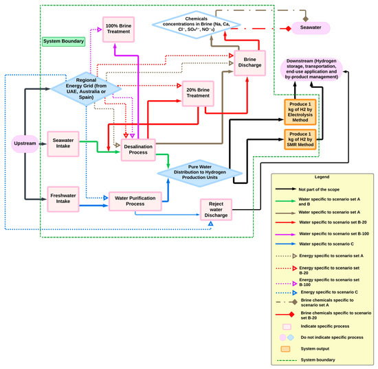
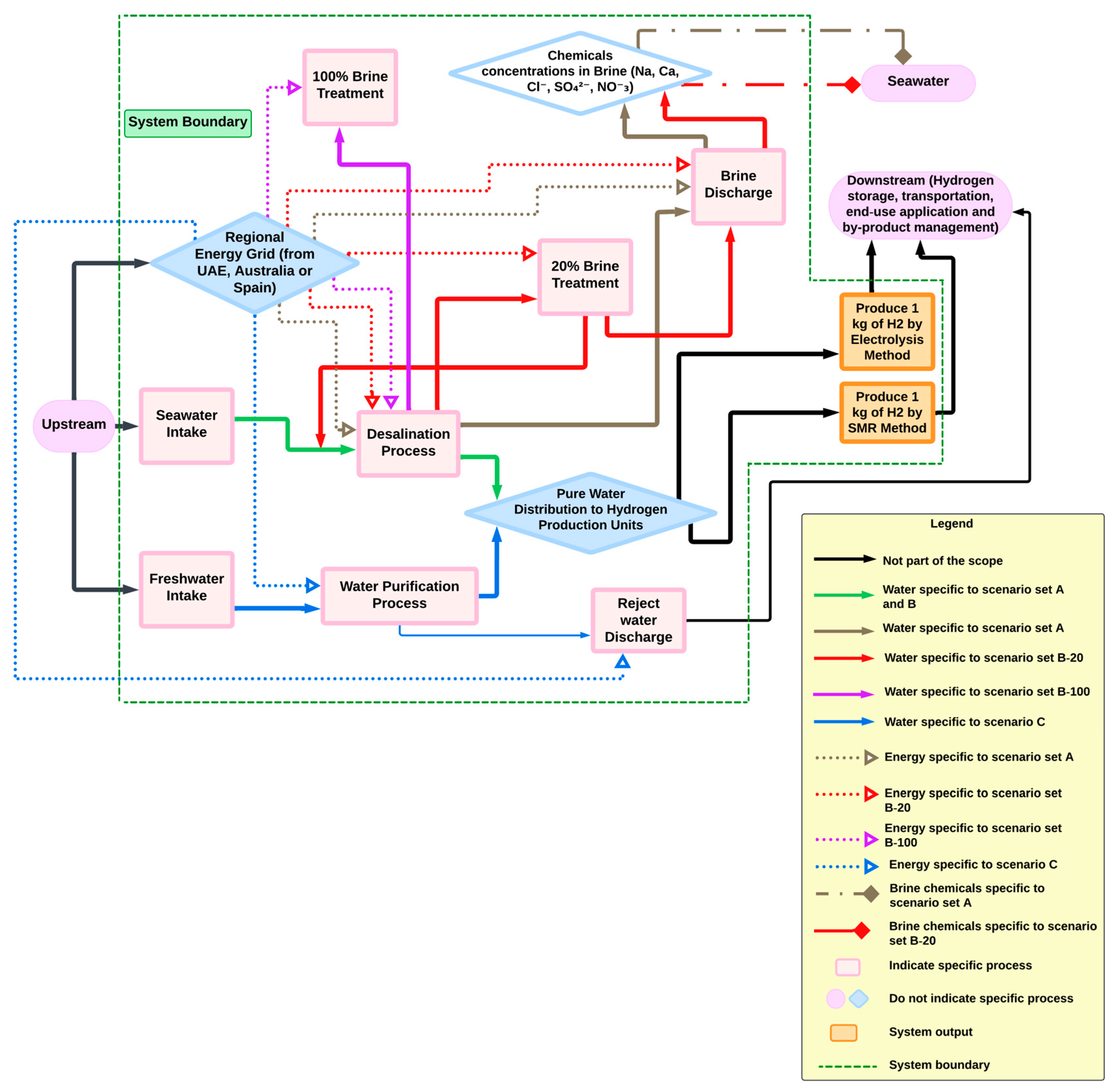

Disclaimer/Publisher’s Note: The statements, opinions and data contained in all publications are solely those of the individual author(s) and contributor(s) and not of MDPI and/or the editor(s). MDPI and/or the editor(s) disclaim responsibility for any injury to people or property resulting from any ideas, methods, instructions or products referred to in the content. |
© 2026 by the authors. Licensee MDPI, Basel, Switzerland. This article is an open access article distributed under the terms and conditions of the Creative Commons Attribution (CC BY) license.