Article

Analyzing the Applicability of Random Forest-Based Models for the Forecast of Run-of-River Hydropower Generation

1
MINES ParisTech, Centre de Mathématiques Appliquées (CMA), Sophia Antipolis, 06560 Paris, France
2
Université Côte d’Azur, Inria, CNRS, 06560 Sophia Antipolis, France
3
LNEG—Laboratório Nacional de Energia e Geologia, I.P. Estrada da Portela, Bairro do Zambujal Ap 7586, 2610-999 Amadora, Portugal
*
Author to whom correspondence should be addressed.
Clean Technol. 2021, 3(4), 858-880; https://doi.org/10.3390/cleantechnol3040050
Submission received: 1 October 2021 / Revised: 17 November 2021 / Accepted: 15 December 2021 / Published: 20 December 2021
(This article belongs to the Special Issue AI in Clean Energy Systems)

Abstract

:
Analyzing the impact of climate variables into the operational planning processes is essential for the robust implementation of a sustainable power system. This paper deals with the modeling of the run-of-river hydropower production based on climate variables on the European scale. A better understanding of future run-of-river generation patterns has important implications for power systems with increasing shares of solar and wind power. Run-of-river plants are less intermittent than solar or wind but also less dispatchable than dams with storage capacity. However, translating time series of climate data (precipitation and air temperature) into time series of run-of-river-based hydropower generation is not an easy task as it is necessary to capture the complex relationship between the availability of water and the generation of electricity. This task is also more complex when performed for a large interconnected area. In this work, a model is built for several European countries by using machine learning techniques. In particular, we compare the accuracy of models based on the Random Forest algorithm and show that a more accurate model is obtained when a finer spatial resolution of climate data is introduced. We then discuss the practical applicability of a machine learning model for the medium term forecasts and show that some very context specific but influential events are hard to capture.

1. Introduction

The European community called for fully decarbonized power generation by 2050. Achieving this goal means that 80% to 100% of the EU’s electricity will be produced by renewable energy sources. Fortunately, as shown in several studies [1], the integration of high levels of renewable energy in the existing power grid in many countries seems to be technically and economically feasible. However, this growth of the renewables share in the existing power systems will likely be driven by very intermittent solar and wind resources and will require a more flexible and smarter electric power system management.
Among the renewable sources, hydropower has been identified as highly valuable for climate mitigation due to its low carbon footprint, high generation efficiency, reliability, and flexibility. For this reason, installed hydropower capacity continues to grow quickly to empower the transition towards climate neutrality. During the year 2020, 21 G W of hydroelectric capacity was put into operation worldwide ( 1.6 % more than 2019). Hydropower capacity rose by 3 G W in Europe [2], and continues being the European most dominant source of renewable electrical energy. Table 1 reports the top fifteen European countries by installed (run-of-river and reservoir) hydropower capacity, together with the total hydropower generated in 2020.
Hydropower plants can have low hydraulic heads and small reservoir (RoR) or can include large water reservoir with hydraulic heads up to several hundred meters (Res). In this second case, water recirculation between lower and higher levels can be possibly implemented by pump-storage systems. Among these existing technologies, we focus on the ‘pure’ run-of-river-based one, which is more directly affected by the daily patterns of climate variables. RoR plants exist alongside rivers and do not contain large reservoirs to store or regulate the flow of the adjacent river. Typically, they generate electricity according to the water flow. This latter is defined by seasonal patterns of precipitation, evaporation, drainage, and other characteristics, which all depend on the geography and climate peculiarity of locations [3]. Although the seasonal patterns of wet and dry seasons are relatively predictable, they are not guaranteed and can vary from one year to another [4]. Within a given season, output of RoR plants can then be impacted by the daily rivers discharge levels.
RoR plants are generally not operated in compliance with the power system’s needs, as is done for the conventional fossil fuel power plants, due to the variability of the ‘fuel’ supplying the hydropower generation. However, mathematical models can be introduced for helping the analysis of the impact of climate variables on hydropower generation. In particular, reliable models can be used to provide accurate forecasts of the hydropower availability based on possible climate variable time series. This useful tool supports the integration of the RoR hydropower generation into the scheduling planning process of electricity generation.
In the literature, the impact of climate variability and change on hydroelectric production is usually evaluated by using hydrological models, such as IHACRES [5], HBV M [6], and GEOTRANSF [7]. The inputs to these models usually include time series of meteorological variables (e.g., precipitation, temperature, and solar radiation) and physiographic information of the power plants locations (e.g., characteristics of surface water bodies, soil type, and topography). For every location of interest, when all these data are available and the model parameters are calibrated, hydrological models accurately represent the rainfall–runoff relationship. Finally, the transformation from the river runoff to hydropower production requires additional information about the power plants under investigation (e.g., hydraulic head). When not all the required inputs are available for calibrating a hydrological model, future hydropower projections are usually computed as the long-term mean over the past years. However, the link with observable climate variable is then lost. Indeed, with more initiatives aiming at a greater availability of climate variable forecasts for the next season, building such a model could not support the decision-making process.
For our work, we have the availability of the following data:
  • time series of climate data (precipitation and temperature),
  • time series of the hydropower production at level of a country, and
  • hydropower yearly installed capacity.
With the above inputs, we aim at building a model able to catch the relationship between climate variables and hydropower capacity factor (CF), that is, a fraction of the produced power over the installed one. In this paper, we investigate the use of Machine Learning (ML) techniques for building such a model. Differently from a hydrological model, machine learning does not require a detailed knowledge of the technical design of individual plants.
In the literature, it is shown that ML methods are well-suited to the domain of wind speed and wind power prediction [8,9] as well as for solar radiation and solar production [10]. ML techniques were also applied to the run-off forecast, see in [11] and references therein, but at the best of our knowledge, a little attention is dedicated in the literature to the prediction of run-of-river hydropower generation from climate data. The reason for this lack could be due to the fact that, while the spatial-temporal relation between wind speed–wind power generation (solar radiation-solar power) is local [12], the one between climate variables, river run-off, and hydropower generation is much more complex due to the coexistence of several spatial and temporal scale conditions. An example is the determination of the temporal relation between the generation and weather event. Indeed, the impact of the climate variables on the water flow, and the corresponding power production, may occur with a certain delay, whose determination depends on physically-based phenomena. For instance, the melting process of the snow at a high altitude requires a certain amount of time, which depends on the local air temperature. Therefore, the water flow increment due to the snowfall during the winter may occur only after many months as the temperature increases. However, due to climate changes, such delay is not easily predictable.
The recent paper [13] also applies ML for the modeling of hydropower CF based on climate data. Although we share with that paper the aim and the ML algorithm used, there are significant differences. The first is the selection of the climate dataset. We use a dataset provided by Deutscher Wetterdienst (DWD) [14]. In [13], only the country average of the climate data is considered. Instead, we show here that a better performance can be obtained when climate data with a finer spatial resolution are included in the predictors for the ML models. The authors also calibrated their ML on the full dataset and used the model as a backcasting tool to generate past hydropower output time series. We focus instead on daily predictions for the medium season. Our focus here is to better understand how such models can provide useful insight to the power sector, or what we can learn from the prediction errors. We thus discuss the prediction errors and some modeling challenges such as country specific issues that make the prediction difficult. This finally leads us to evaluate the limits and applicability of ML for operational forecast of the expected electricity output for the next season or year.
The structure of the paper is as follows. In Section 2, we give details about the data that feed the ML models. Section 3 is dedicated to the presentation of the procedure used to build the three models considered in this paper. Models’ comparison and evaluation are presented in Section 4. In that section, we also discuss the practical applicability of the ML model when used for the prediction of the one-year ahead capacity factor. Finally, conclusions and a few hints for future research are presented in the last section of the paper.

2. Materials

2.1. Climate Input Data

Climate data include the time series of precipitation and near surface air temperature with a spatial resolution in the atmosphere about 0.95° on Europe (50° N) and 95 vertical levels reaching up into 80 km height. These data are produced by using a data assimilation technique described in [15]. As mentioned, these data covering the period 1995–2019 are provided by Deutscher Wetterdienst (DWD) [14]. Although the data are available in six-hour temporal resolution, we use the daily resolution for this study. Forecasting aggregated daily capacity factors is preferred to leave more flexibility to the intraday hourly dispatch. Concerning the spatial resolution, we aggregate climate data to NUTS2 level (i.e., statistical regions for the application of regional policies [16]) or to country level.

2.2. Hydropower Production and Installed Capacity Data
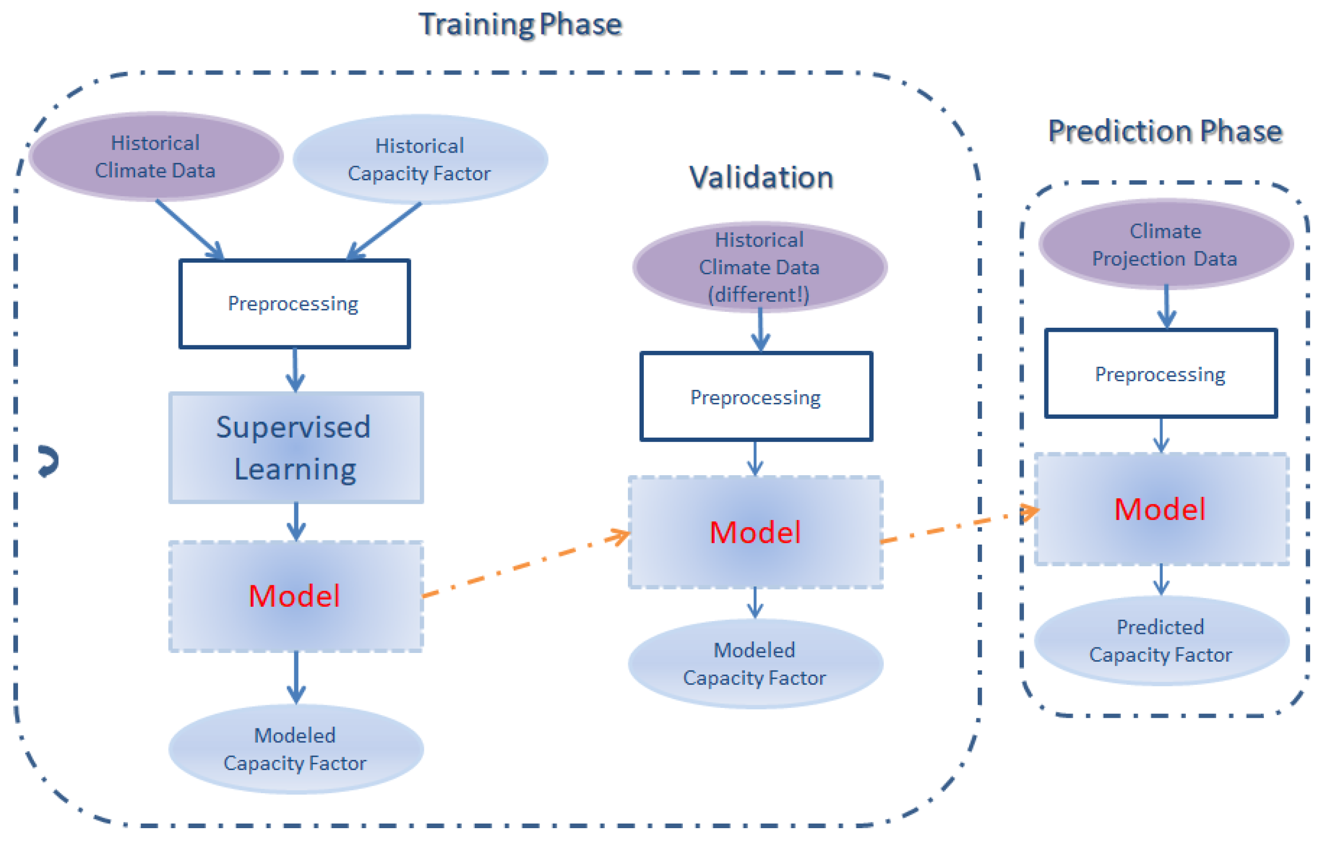
Data of hydropower production aggregated at country level are from the ENTSO-E Transparency Platform [17], where energy demand and generation data are systematically collected at hourly time resolution starting from 1 January 2015 to the current days. Among the fifteen countries listed in Table 1, we select the eleven for which data are available at least from January 2016. These are indicated in bold in that table. In order to be consistent with temporal scale of climate data, we compute the daily average value. From the same platform, we also collect the value of the yearly hydropower installed capacity. With this two kinds of information, we can compute the time series of the capacity factor, which is defined as the percentage of hydropower generated over the installed one. Note that for some country, such as Spain and Norway, data of the hydropower generation present values larger than the installed capacity. For this reason, we set as the installed capacity for this country and for the year when this event occurs equal to the peak of hydropower production. Note that differently from the work in [13], we do not consider a fixed installed capacity over all the years for computing the CF. We mention here that the CF is only available at the level of a country.

3. Methodology

3.1. Machine Learning

Machine learning has been gaining more and more importance in many areas of science, finance, and industry [18]. Typically, it is used to predict an outcome based on a set of features. In the case of the present paper, the ML model is built to predict the daily time series of the RoR capacity factor over the coming season based on future daily time series of the climate variables.
The workflow of the ML procedure is given in Figure 1.
The procedure starts by training a so-called (supervised) learner with a set of data, including the observed outcome and feature measurements. This leads to building a model that predicts the unobserved outcome based on a different set of input features of the same kind used in the training phase. A good learner is one that accurately predicts such an outcome. The features are often called predictors or inputs in the statistical literature, whereas the outcomes are called responses or outputs. In this paper, we will make use of all these terms. Based on evaluation metrics including the correlation coefficient, the normalized mean absolute, and the normalized mean square errors, to be defined in Section 3.3, we will compare three models to determine the one with the highest accuracy.
In [19], we performed a preliminary study for selecting the best ML technique for predicting hydropower production from climate data. We compared five regression methods and showed that Random Forests (RF) [20] leads to the best results. Therefore, in this paper, we compare the performance of this algorithm by considering several combinations of predictors. The RF algorithm is based on an ensemble of decision trees. Random vectors are used for growing each tree in the ensemble. A tree is grown by considering a random selection of the training set. Then each tree depends on the values of a random vector sampled independently and with the same distribution for all trees in the forest. The RF algorithm requires setting up some hyperparameters. In our experiments, we set the number of trees equal to 500 and minimum leaf size equal to 5, and we select sampling over all variables. Although theoretically a larger number of trees and a smaller minimum leaf size should improve the accuracy of the model, preliminary tests have shown that the improvements are not significant enough to justify a larger computational effort. The tuning of the rest of the hyperparameters is implemented by the optimization procedure offered by MATLAB Machine Learning toolbox 11.4 [21] along with the trial and error approach.

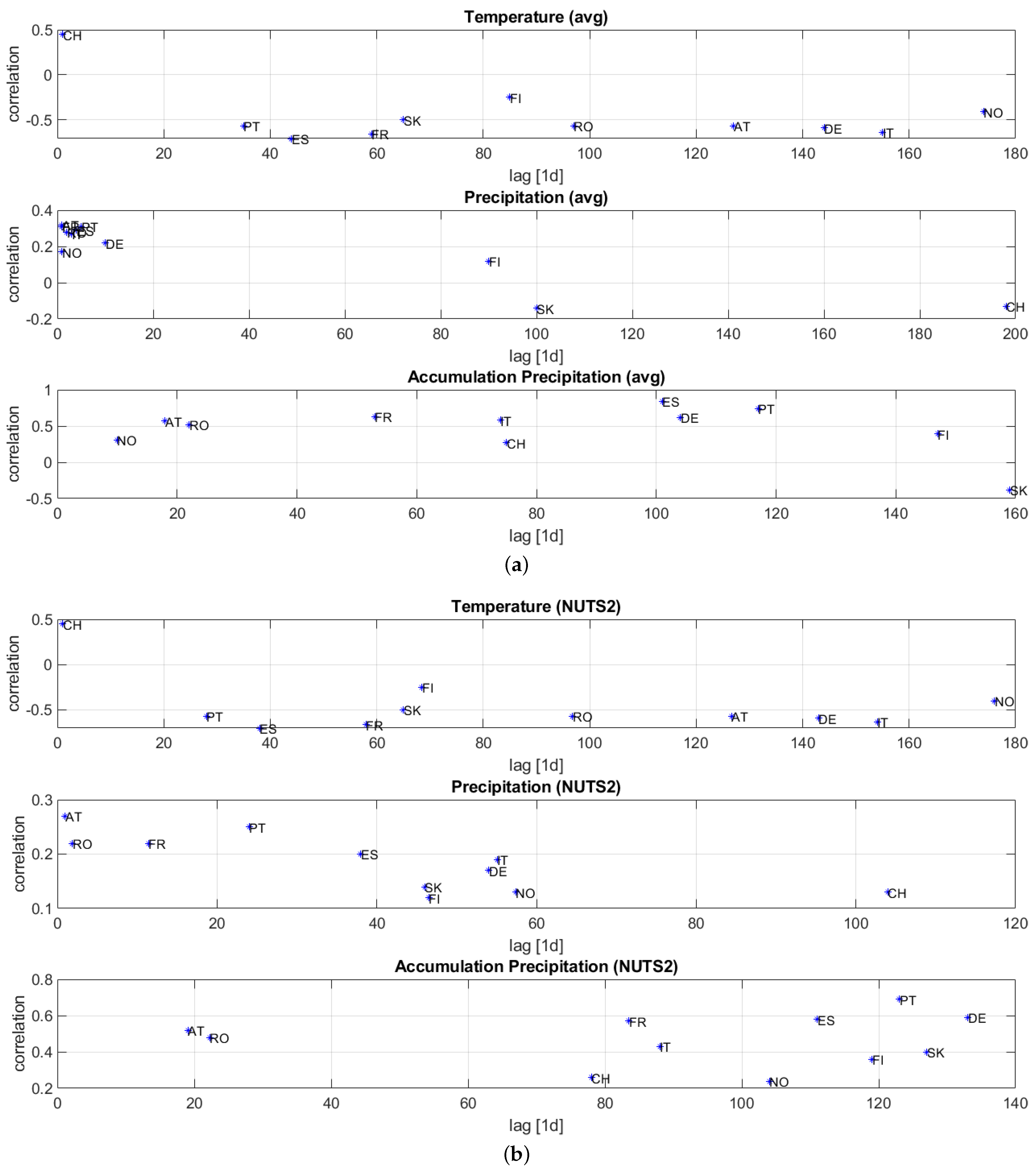
3.2. Choice of the Predictors

The experiments aim at formalizing the model with the best accuracy for predicting the RoR hydropower daily capacity factor for the EU countries listed in bold in Table 1.
The first step in the ML workflow is the training phase. Let us indicate with T train = { t 1 , , t j , , t N } a given daily spaced time interval, where t 1 and t N are, respectively, the initial and final date. We assume that over the training period we collect the data corresponding to
  • air temperature, i.e., the time series A T = [ A T t 1 , , A T t N ] ;
  • precipitation, i.e., the time series T P = [ T P t 1 , , T P t N ] ; and
  • capacity factor of hydropower generation, i.e., the time series y = [ y t 1 , , y t N ] .
As we explained above, the effects of the climate data on hydroelectricity generation occur with a certain delay, which also depends on the location of the climate event. In order to take this observation into account, we enrich the list of inputs by considering that the hydropower generation at a day t i is also influenced by
  • the air temperature at the preceding k 1 -th day with respect to t i , where k 1 is computed by considering the lag that maximizes the sample Pearson correlation [22] between the time series of the hydropower generation y and of the air temperature A T , say ρ ( y , A T ) ;
  • the precipitation at the preceding k 2 -th day with respect to t i , where k 2 is computed similarly to k 1 by considering ρ ( y , T P ) ; and
  • the sum of precipitation in the last k 3 days with respect to t i , with k 2 defined as explained above.
The above procedure is called optimal lags in [23]. In this paper, we show the effect of introducing a finer spatial resolution for temperature and precipitation at NUTS2 level. Therefore, different lags are defined for the different NUTS2 climate data. Moreover, depending on the country, not all the above inputs are relevant for the prediction of the hydropower CF. Then, in order to choose if a certain time series is used as input to the RF algorithm, we compute the correlation, ρ , between the time series of each above input and the response over the training period [24]. Then, a time series is added to the list of predictors if | ρ | is bigger than a certain threshold ρ ¯ . This choice was implemented as we observed that adding inputs whose correlation with the response is lower than a chosen threshold does not improve the prediction in terms of the evaluation criteria to be presented below.
Once the predictors are selected, they are used for training a learner. The accuracy of each model is assessed by performing a classical 5-fold cross-validation [18] and by computing the values presented in the next section.

3.3. Model Validation
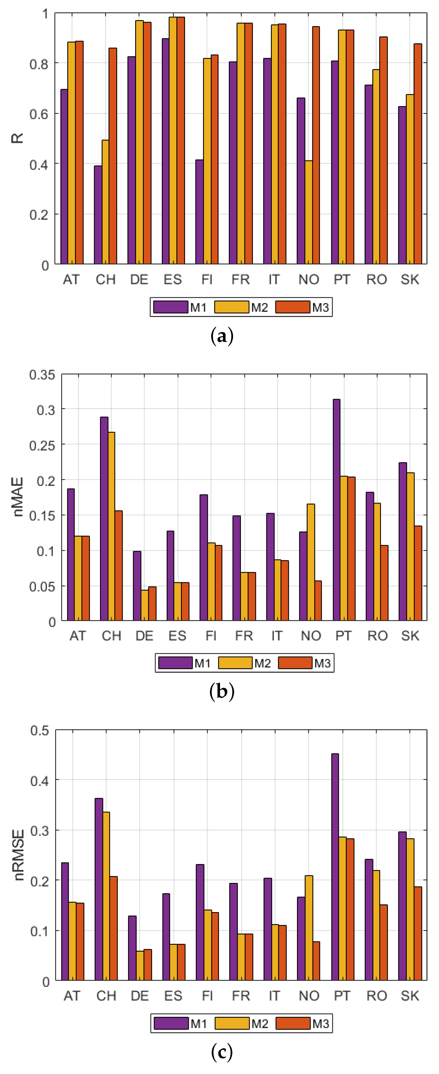
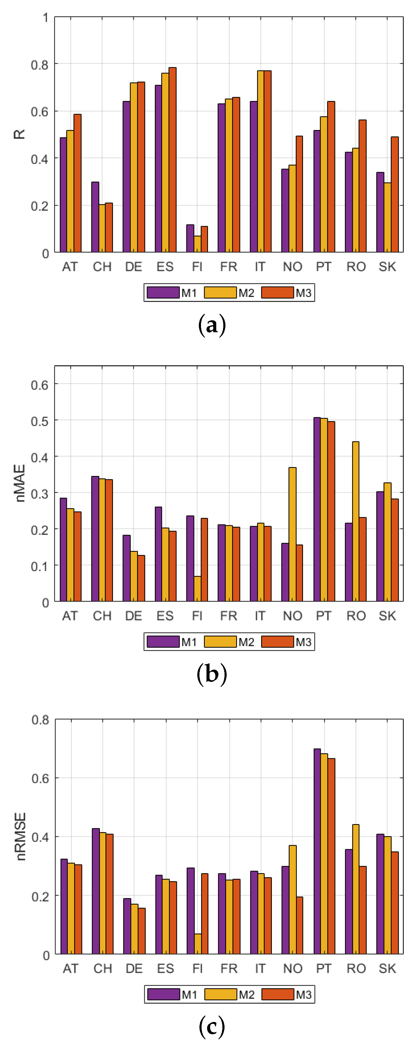
In this section, we describe the measure used in the validation phase. We call T test = { τ 1 , , τ M } this daily spaced time interval, and we indicate with y ¯ = [ y ¯ τ 1 , , y ¯ τ M ] the time series of the observed CF over this testing period. Note that we set the lags k i , i = 1 , 2 , 3 to the values computed in the training phase. The main difference here is that the input list does not include the time series of the hydropower CF, which instead will be the output of this phase.
From now on, we will use the term ‘modeled’ instead of ‘predicted’ output for the results of the ML process, which we indicate as y ^ = [ y ^ τ 1 , , y ^ τ M ] . It is important to highlight that the testing period is distinct from T train and that y ¯ is not used as input to the model, but it will be used only for purpose of comparison.
For the performance evaluation of the models used in this paper, we consider the following measures:
  • Correlation coefficient (R)
    R = c o v ( y ¯ , y ^ ) σ y ¯ σ y ^ ,
    where c o v is the covariance, and σ y ¯ and σ y ^ are the standard deviation of y ¯ and y ^ , respectively. It is a measure of the strength and direction of the linear relationship between the observed and the modeled variables.
  • Normalized Mean Absolute Error ( n M A E )
    n M A E = i = 1 M | y ^ i y ¯ i | i = 1 M y ¯ i .
    Note that the normalized version of MAE is preferred in this case as the actual CF may include also zero or close to zero values, then the classical mean absolute percentage error would lead to large error values.
  • Normalized Root Mean Square Error ( R M S E )
    n R M S E = R M S E 1 / M i = 1 M y ¯ i ,
    where R M S E = 1 M i = 1 M ( y ^ i y ¯ i ) 2 .

4. Results

This section first describes the ML models considered in this paper. Then a classical 5-fold cross validation is used to select the model providing the best performace. As further validation for the model selection, we also perform a leave one year out validation. Then the model showing the best performance in those validation procedures is used for the prediction of the one-year-ahead capacity factor. Finally, we discuss how to extract practical information for the ML model’s error to be integrated in an energy system model.

4.1. Model Selection

Table 2 shows the list of features considered in this paper. The definition of each model is based on the selection of the inputs passed to the RF algorithm.
Climate data are averaged at country level in model M1 and at NUTS2 level in model M2. A combination of these two types of inputs is implemented in model M3.
The selection of the lags for the climate time series in M1 is similar to that proposed in [23] where only an average aggregation is considered. As explained in Section 3.2, for the other models, we select only a subset of the NUTS2 climate time series based on their correlation with the response over T train . Our numerical experiments indicate that a threshold correlation ρ ¯ = 0.5 seems to be a good compromise between the number of selected predictors and the accuracy of the solution. Figure 2 reports the values of the optimal lags selected for the predictors in the ML models computed considering the maximum correlation between each climate and energy time series over the period 2015 to 2019. When NUTS2 data are used, as in M2 and M3, an optimal lag for each NUTS2 time series is computed. For matter of space, in Figure 2b, we only show the average lag values. More details are reported in Table A1 in Appendix A.1.
Figure 3 shows the values of the metrics presented in Section 3.3 obtained by implementing a 5-fold cross-validation [18]. We can observe that a more accurate model is obtained for all countries when only selected NUTS2 climate time series are chosen. This shows that a significant improvement is achieved when climate data with a finer spatial resolution are used.
As there is still some information in the average climate data which could improve the accuracy, we implemented M3 combining these two types of inputs. Note that the average and a subset of NUTS2 climate data are not truly redundant, and their simultaneous use as inputs can improve the model accuracy [24]. Indeed, the results in Figure 3 confirm this conjecture. Therefore, we select model M3 and evaluate the accuracy of the out-of-bag 5-fold cross-validation values.
In Figure 4, we report quality measures for evaluating the performance of the selected model for reproducing the observed time series of the CF. In particular, we show the values of the variance and the quantiles of the corresponding time series. From this figure, we can see that M3 can well reproduce the observed time series variance for all countries, but, in general, it tends to overestimate minimum values and underestimate the maximum. As a result, the range of values spanned by the modeled CF is narrower than the observed one. On the other hand, we can observe that the values of 25 % , 50 % , and 75 % quantiles are well reproduced by M3. The numerical values of these measures are also given in Table A2 in the Appendix A.2.
Finally, in Figure 5, we report the scatter plot of the out-of-bag 5-fold cross-validation output of M3 and the observed CF. In those figures, we indicate with blues dots the CF values in the period December–January–February (DJF), with orange circles the values in the period March–April–May (MAM), with red dots for June–July–August (JJA) and, finally, with green circles for September–October–November (SON). We can see that the modeled CF is, in general, quite close to the observed data. For countries with a relevant installed capacity (>9 G W ), such as Italy and France, we obtain a correlation coefficient equal to 0.96 and 0.95, respectively. Note that these values drop to 0.88 and 0.86 when only the mean values of the climate data are used as predictors. The worst fit ( R = 0.72 ) is obtained for Switzerland, which is interestingly the country with the smallest RoR installed capacity among the ones considered in this paper. Note also that the hydropower data for CH were collected starting from 2016, that is, a smaller training period is available. Moreover, in Figure 5, we can observe a cloud of red points corresponding to high values of CF in the summer period of 2019. This occurrence was not observed in the past years and, for this reason, it could not be ‘learned’ by our model.
As a further comparison, we evaluate the performance of the three models in predicting a one-year time series by training and testing over different time slices. Each row in Table 3 shows the data used in the training and testing phases for each model, amounting to 80 % and 20 % , respectively. For instance, the first row says that we train each of the three models over the period 2016 to 2019, and we use the year 2015 for testing. We train and test the RF algorithm five times for each model, and, as a result, we obtain a time series of the modeled CF covering the five years considered, and all being ‘out-of-sample’ data.
As shown in Figure 6, the performance of all models is lower in this case. This was expected as the RF algorithm tends to perform better on the out-of-bag k-fold validation [25]. However, these results confirm the trend observed before. Indeed, by comparing the values of R, nMAE, and nRMSE corresponding to M1 and M3, we can observe that the contemporary use of the mean value and a selected subset of NUTS2 climate time series leads to an increase of 7 % of the average correlation coefficient, and a decrease of 7 % and 10 % in nMAE and nRMSE, respectively.

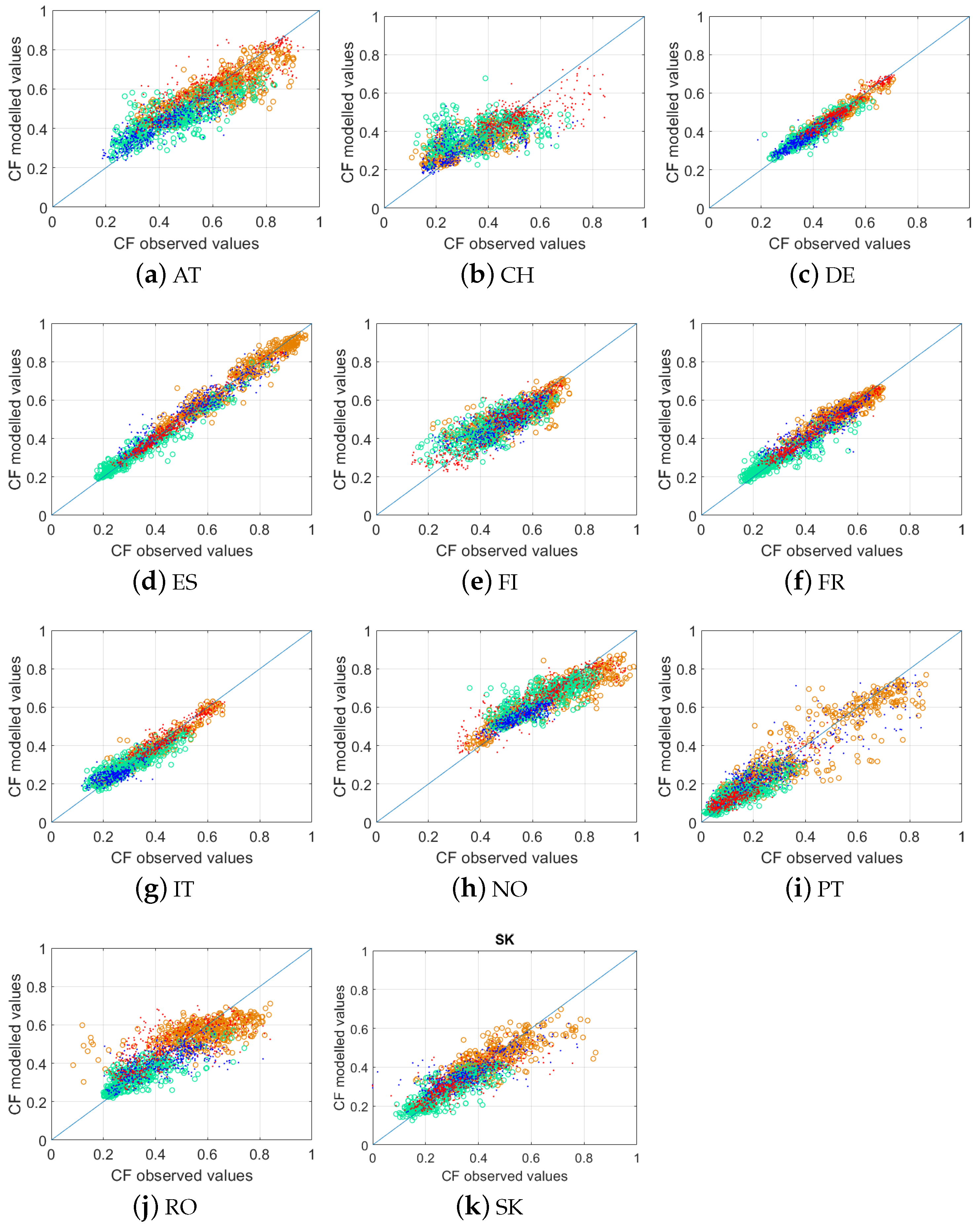
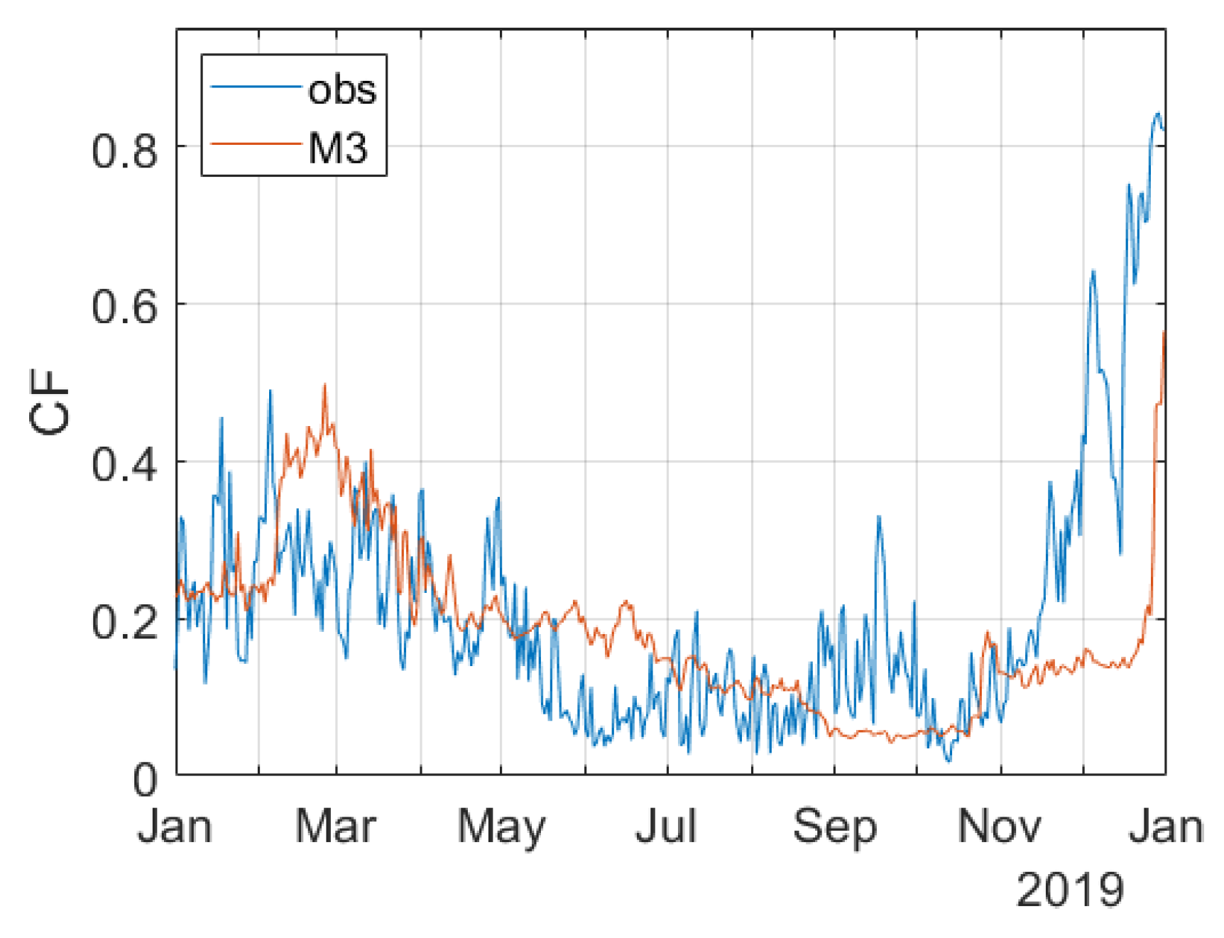
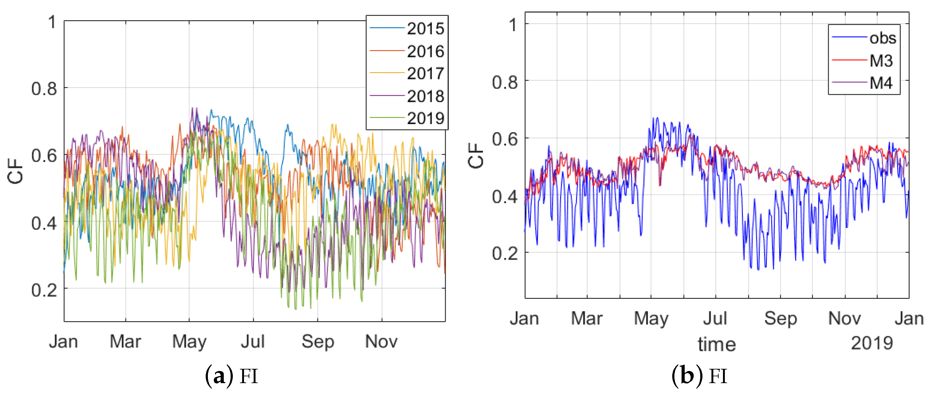
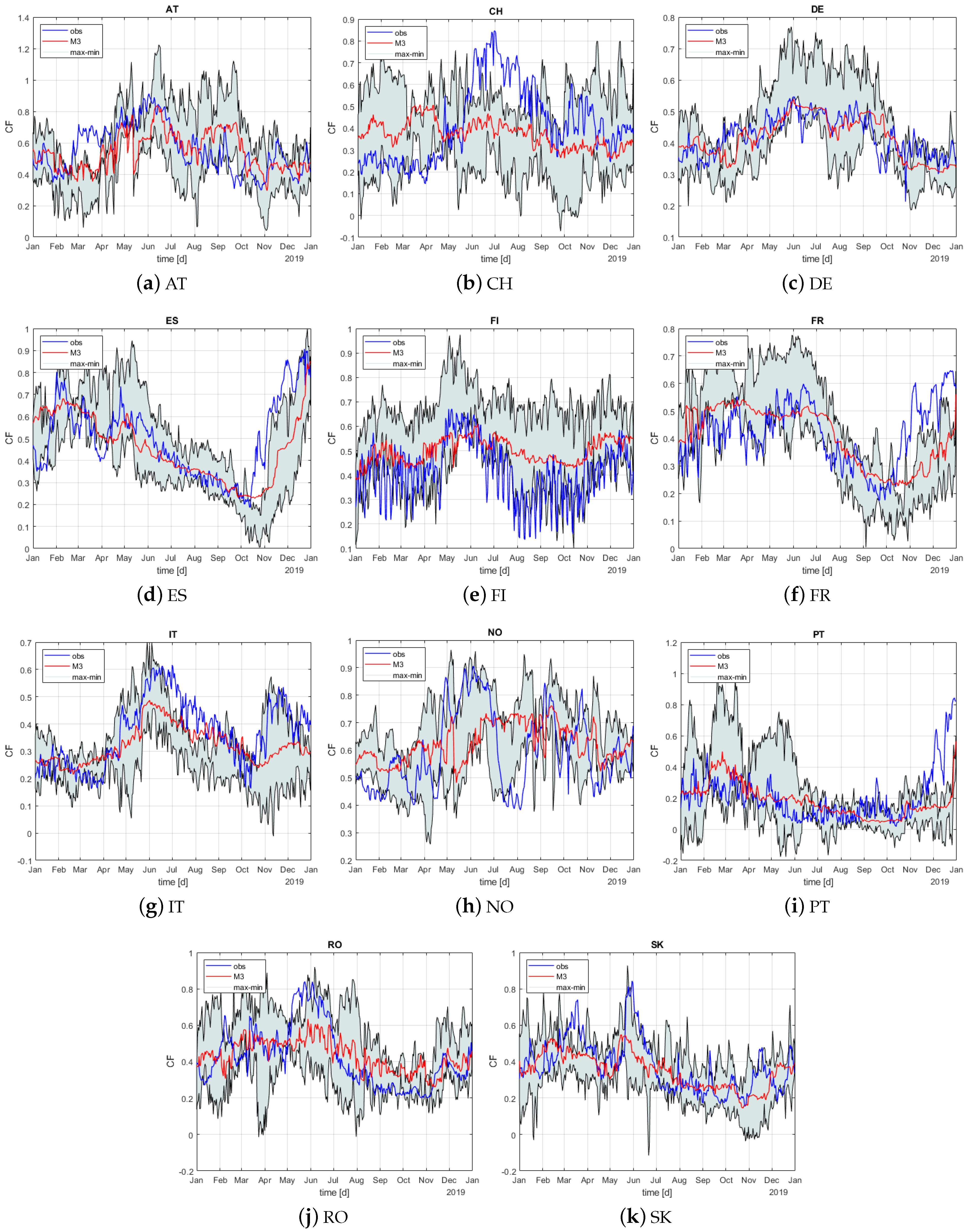
4.2. Accuracy of Prediction

The main goal of the ML model formalized in this work is to be used to perform medium term predictions. This means that we predict daily time series of the hydropower CF one year ahead of the most recent observation of the predictors. With this in mind, in what follows, we assume to train model M3 over the interval 2015 to 2018, and perform a ‘prediction’ over 2019. The following evaluation of this model comes as an example to present possible issues that could be met when this kind of models are used for performing future predictions.

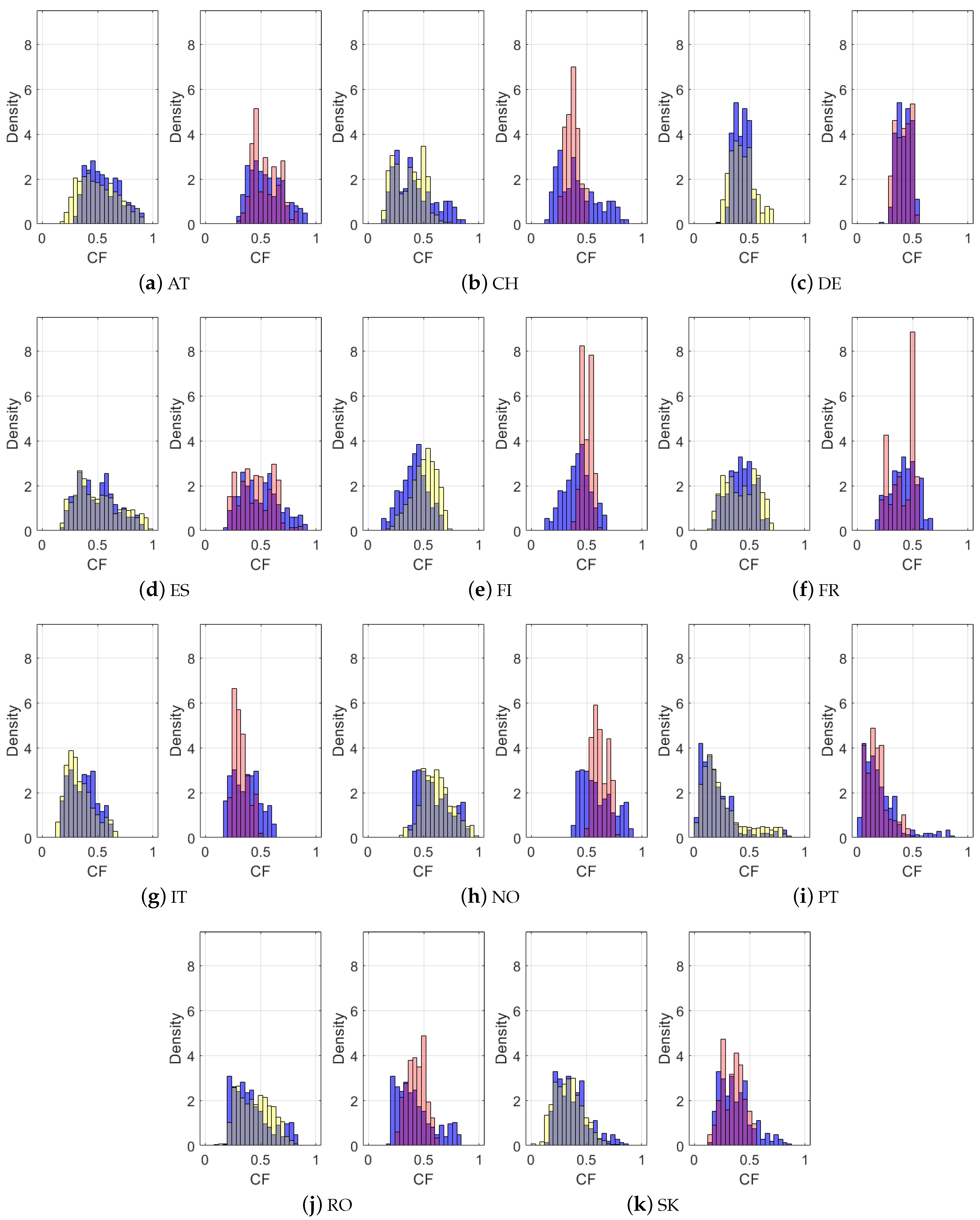
4.2.1. Modeling Challenge: Representativeness of the Training Set

In Figure 7, for each country, in the leftmost panels, we compare the distribution of the observed CF in 2019 (blue) and the distribution of observed CF over the interval 2015–2018. This figure allows understanding the difficulties in predicting the values of CF in 2019 as the values spanned by the CF in the training and testing intervals are quite different, see, for instance, the cases of Austria, Germany, and Finland. In the rightmost panels, we compare the total distribution of modeled and observed time series over the year 2019. As already mentioned above, our model tends to estimate a narrow range of CF values. For this reason, we observe a higher density in the intermediate values for the modeled CF.

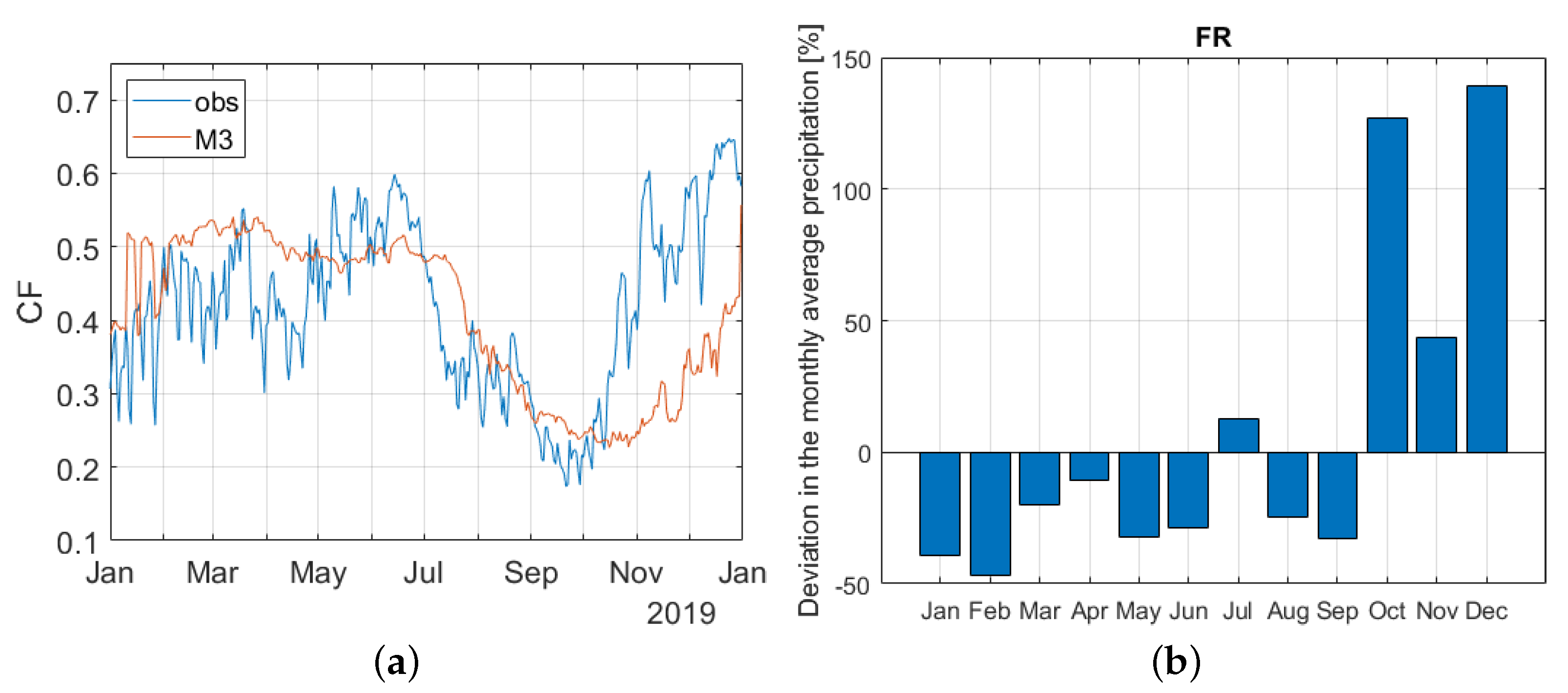
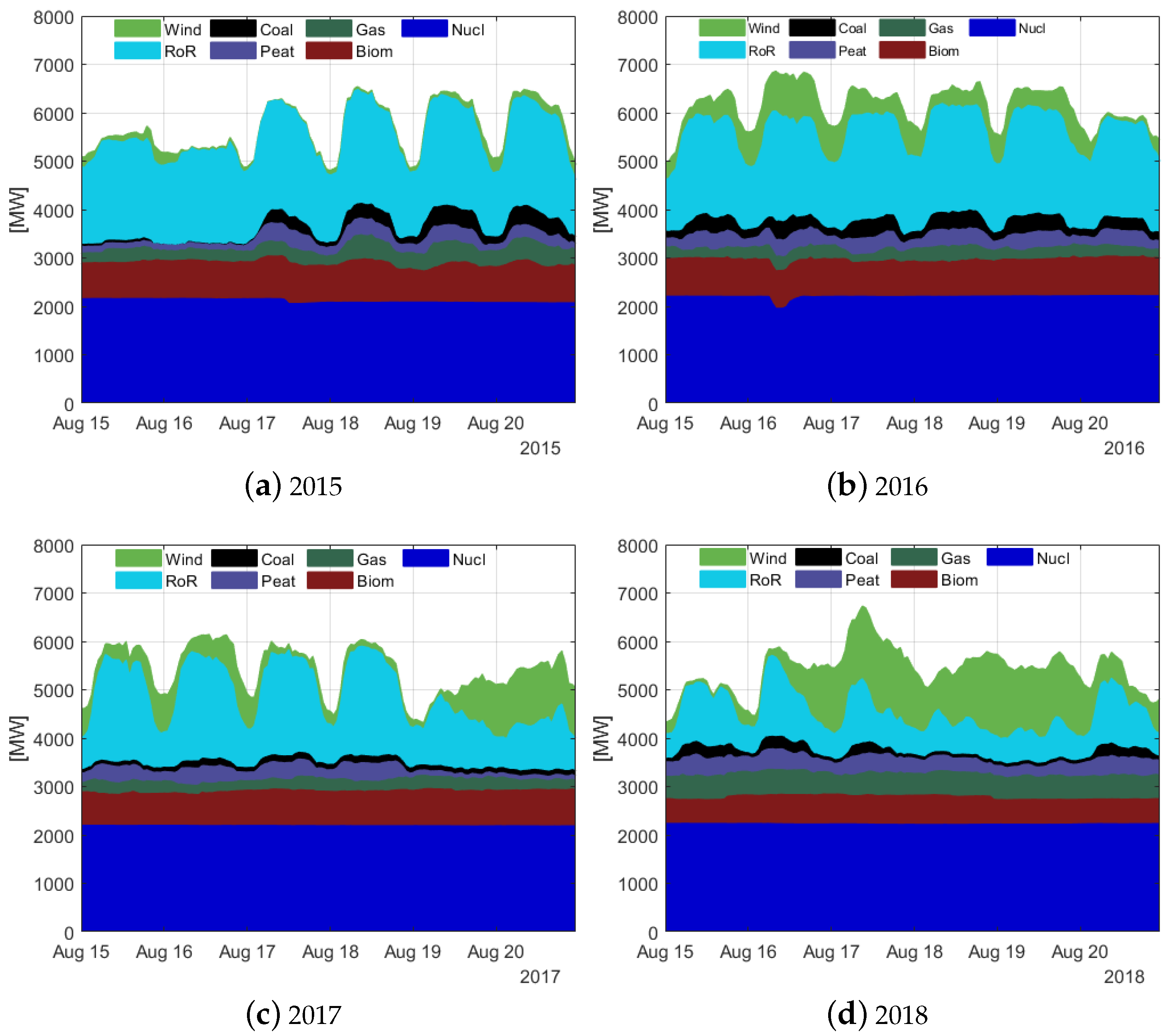
4.2.2. Modeling Challenge: Insights on Country Specific Issues

France: Autumn’s heavy rainfall
When we use the routine shown in Table 3 for predicting the CF over one entire year, we collect the values of R, nMAE, and nRMSE corresponding to each of the five years considered. The best fit we obtained for the year 2018 with R = 0.9, nMAE = 0.17, and nRMSE = 0.2, whereas for 2019 we observed a drop in the accuracy with a correlation coefficient R = 0.44, nMAE = 0.22, and nRMSE = 0.28. In this section, we explore a possible reason for such a discrepancy in the prediction performance.
Figure 8a reports the time series of the observed CF (blue line) and the modeled CF (red line). As said, the overall accuracy of the modeled CF is low and in particular, model M3 could not predict the CF corresponding to the last part of the year. To explain that, we looked at the deviation of the monthly average of the precipitation (at country level) over 2019 with respect to the monthly average over the past years. As we can see in Figure 8b, October and December 2019 in France registered an exceptional amount of precipitation if compared with average of the four previous years (https://surfobs.climate.copernicus.eu/stateoftheclimate/october2019.php, accessed on 1 November 2019). This yielded a fast increase of the RoR CF, which was not ’seen’ by the ML model. Although model M3 has shown to perform quite well for France, so as displayed in Figure 3 and Figure 6, the prediction ability is limited to events which are included in the training set.
Portugal: trans-boundary challenge
We point out here that an accurate model for the RoR hydropower CF for the Iberian Peninsula, particularly for Portugal, is quite hard to build. Indeed, Spain and Portugal share three of the largest rivers in the Iberian Peninsula, and, being upstream, Spain generates 70 % of the annual water resources of these rivers. In order to regulate the water sharing, in 1998 these two countries signed the Albufeira Convention. This Convention establishes the minimum volume of water that Spain must release to Portugal, which is 2700 h m 3 in each hydrological year. However, in the hydrological year 2018/2019, Spain did not honor the agreements and only shared a third of the agreed river flow with Portugal. That, of course, impacted the Portuguese RoR hydropower generation and altered the climate dependency. The modeled CF in Figure 9 shows an underestimation after November and an overestimation before September which could be linked to the combination of lower than average precipitations and the water sharing issue.
Finland: is there any hydropeaking effect?
As illustrated by Figure 10, model M3 performs poorly for Finland (R = 0.48, nMAE = 0.25, nRMSE = 0.32). The comparison of the available training data (i.e., daily value in the interval 2015 to 2018) shows that this could be explained by the fact that there is no clear tendency, and that only 2018 exhibits a low CF capacity factor in August and September. A second peculiarity of the observed CF in Finland (right panel) is the evidence of important daily variations. A possible explanation for such behavior could be the issue of hydropeaking, which is discussed more precisely in [26]. The mechanism at play will then be the occurrence of very irregular river flows due to sudden variations in the output of upstream hydropower reservoirs to balance the system. Reservoir refers in Finland mostly to ‘pondage’ and smaller reservoir for RoR plants. By working with daily capacity factors, we account for the possibility of intraday variation. Cascading of plants here refers to several RoR dams on a single river.
In this paper, the ML models are built assuming that we deal with ’pure’ run-of-river plants. However, as explained above, this assumption may be too restrictive for some specific countries. For this reason, we include the time series of the country average electricity demand as a further input and define M4. Although a slight improvement in the evaluation metrics is obtained (R = 0.56, nMAE = 0.24, nRMSE = 0.31) the modeled CF cannot reproduce the hydropeaking effect.
The demand may not be the only cause of hydropeacking. In fact, further analysis shows that a source of ’unseen’ occurrence in training data may be linked also to the change in the energy mix of this country. As shown in Figure 11, between 2015 and 2018 for the month of August, RoR plants are increasingly operated to compensate the fluctuation of wind power (installed wind capacity was 496 MW in 2015 and increased to 1908 MW in 2018). The balance also incidentally shows that wind replaced more hydropower than coal or natural gas during this episode, pointing potentially to a minimum ‘must run level’ that requires further investigation. As this change happened in 2018, but not in the previous years, then our interpretation is that it makes it more difficult for the ML model to automatically learn. Then, when we test over 2019 (that was not included in the training), the ML model does not perform well.
This observation seems to lead to the conclusion that for some countries the list of predictors should be enriched with more specific information, such as shares of energy, installed capacity, etc. This is left as a subject for future research.

4.2.3. Relevance for Operational Use

To build an estimator of electricity generation from RoR installations for a large geographical area such as the interconnected EU power system, ML techniques undoubtedly provide a very practical alternative to a full set of more precise hydrological models at individual plants level. The previous sections however showed that while an ML model can capture the overall rainfall dependency trend, several factors of operational importance may be hard to generalize with the current set of available time series. We also recall here a methodological point of caution (as discussed in Section 4.2), which is that while cross-validation approaches are important to confirm the choice of a model type, their performance can be misleading as they usually perform better than the models built for predictive purposes. Figure 12 depicts how ML for RoR could theoretically be integrated as useful step in a larger process. We argue here that, as more data become available, an iterative process will improve the performance of the pipeline. In turn, better ML-based tools will be a strong incentive to more systematically explore singular events which might not be labeled as extremes but sufficiently significant to still have a high operational value.
As standalone tools, the tested ML models for RoR output prediction on large geographical areas are not yet precise enough to provide decisive operational insights, but including additional information could improve its usability. We test here a very simple approach which interprets the observed performances during the training phase as plausible systematic error. Concretely, knowing the relative error on the training data set for each past year gives a time series of error that we apply to the ML output. As depicted by Figure 13, the information provided is then the ML output and a corresponding min and max range. The width of the shaded area is season and country dependent, and it reflects the explanatory capacity of the training set.
The cumulative effect of these national modeling attempts can then be assessed by accounting for the installed capacity in each country. Indeed, errors in regions with larger installed capacity will have higher operational impact. As shown in Figure 14, the aggregated forecast error between M3 and the observed output could reach 5 GW. We also distinguished a first range of error accounting for potential cancellation of errors between countries (light blue) and a more conservative range that sums the maximum error for each country (grey). Thus, despite important challenges and a lack of longer time series, we believe that complementing the output from ML with indications about the scale of prediction errors and their possible sources is critical to provide useful insight for seasonal to year ahead forecasts.

5. Discussion and Conclusions

Europe is expected to strongly expand its wind and solar power capacity by 2050 to meet its climate goals. In an interconnected system, balancing these highly intermittent sources by hydropower will also involve a European-wide evaluation of the variability of hydropower generation for future climatic conditions.
The methodological framework described in this paper aims to contribute to this issue by translating time series of climate variables into time series of hydropower capacity factor. In this paper, we use the potential of machine learning to obtain such a model. Two main reasons justify the relevance of using this methodology.
First in this analysis, we are not interested in providing detailed results in terms of local hydropower production, but our objective is to model the climate dependency of run-of-river hydropower production at the more aggregated country, then EU levels. Second, machine learning offers the great advantage of extracting useful information without explicitly modeling the phenomenon (e.g., location, hydraulic head, and potentially cascading plants) involved and thus requires fewer data.
We investigated the performance of several models based on the classical Random Forest algorithm. Recent works showed that this algorithm lends itself well for modeling the hydropower capacity factor from climate data. Our experiments showed that a more accurate model is obtained for our dataset when we introduce a finer spatial resolution for the inputs. The performance varies greatly across countries and seasons. Using this model, we then discussed the applicability of the ML output for year ahead forecast. We observed that the current level of accuracy of the ML outputs for all the countries is likely not precise enough to give a strong operational advantage. However, trying to understand the reasons for poor performance for specific countries outlined the length of existing time series and the influence of singular events as plausible explanations. On one side, machine learning does not require numerous diverse inputs for building a model between climate variables and hydropower production, on the other hand, more historical data would be necessary for opportunely training the learners and improve the model accuracy and response to extreme or singular events that have a better probability to be incorporated as the training dataset improves. Although this is an important issue now, it may be naturally fixed with time, and the methodology used in this paper will still hold and earn more value.

Author Contributions

Conceptualization, V.S., E.A., M.B. and S.G.S.; developed code, analysis and validation, V.S.; investigation V.S., E.A.; writing—original draft preparation, V.S.; writing—review and editing V.S., E.A. and M.B.; project admistration, E.A. and S.G.S.; funding acquisition E.A. and S.G.S. All authors have read and agreed to the published version of the manuscript.

Funding

This research was supported by the Europen Clim2power project. Project CLIM2POWER is part of ERA4CS, an ERA-NET initiated by JPI Climate, and funded by FORMAS (SE), DLR (DE), BMWFW (AT), FCT (PT), EPA (IE), ANR (FR) with co-funding by the European Union (Grant 690462).

Data Availability Statement

Climata data are provided by Deutscher Wetterdienst (DWD) [14] and are from their https://esgf.dwd.de/search/clim2power/, accessed on 1 December 2020. Data of hydropower generation and installed capacity are from [17]. More details are presented in Section 2.

Conflicts of Interest

The authors declare no conflict of interest.

Abbreviations

The following abbreviations are used in this manuscript:
MLMachine Learning
RFRandom Forest
RoRRun-of-River
ResReservoir
CFCapacity Factor

Appendix A

Appendix A.1. Optimal Lags in Model Training

In Table A1, we report the values of the optimal lags used in the ML models for the time series of temperature (AT), precipitation (TP), and accumulation of precipitation (Acc TP). The computation is performed by considering climate and energy daily time series data over the period from 2015 to 2019. When the climate data are aggregated at NUTS2 level, an optimal lag for each of the time series is computed. In the first set of columns, titled ‘NUTS2 features’, we report the minimum (min), average (avg), and maximum (max) values of the optimal lags of these NUTS2 time-series. Note the wide range of optimal lags selected for different NUTS time series, highlighting the distinct contribution provided by climate data in different country areas. The second set of columns, named ‘avg features’, shows the optimal lags when climate data are aggregate at country level.
Table A1. Optimal lags (in day) used in the ML models.
NUTS2 FeaturesAvg Features
CountryATTPAcc TPATTPAcc TP
MinAvgMaxMinAvgMaxMinAvgMax
AT126126.661281111819.1123127118
CH11167104.71198717889119875
DE143143.63144154.7815640133.1520014410104
ES93846238.9410223111.35200444101
FI5268.5085146.509136119.251478590147
FR4458.5979111.401032083.5915459153
IT140154.76161155.141982387.90200155374
NO174176.71184157.421985104200174110
PT1828.8035424.40103113123.60131355117
RO9696.879711.8721722.253297222
SK6565651466319127.7517665100159

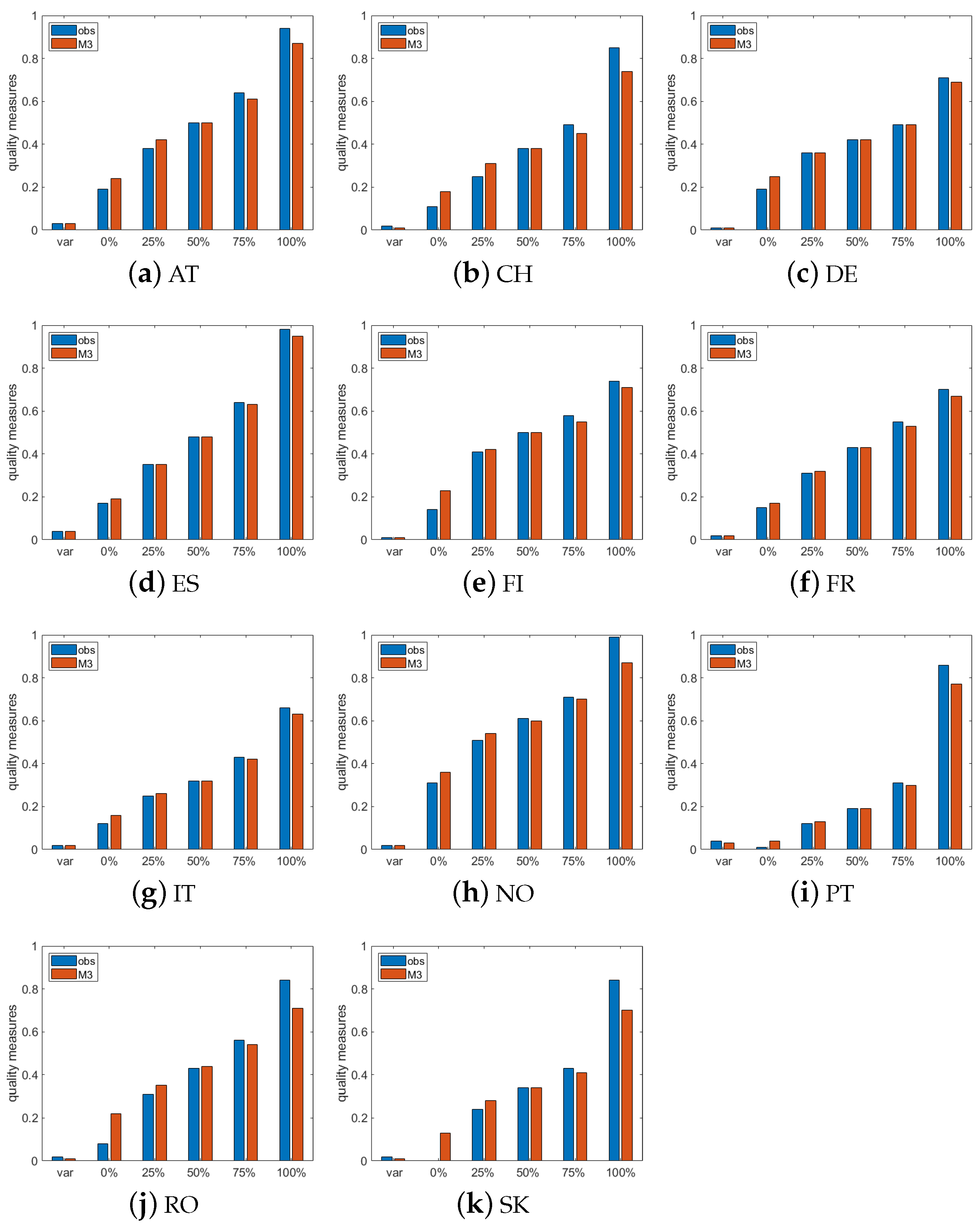
Appendix A.2. Time Series Quality Measures

Table A2. Time series quality measures.
ObservationsM3
Var0%25%50%75%100%Var0%25%50%75%100%
AT0.030.190.380.500.640.940.030.240.420.500.610.87
CH0.020.110.250.380.490.850.010.180.310.380.450.74
DE0.010.190.360.420.490.710.010.250.360.420.490.69
ES0.040.170.350.480.640.980.040.190.350.480.630.95
FI0.010.140.410.500.580.740.010.230.420.500.550.71
FR0.020.150.310.430.550.700.020.170.320.430.530.67
IT0.020.120.250.320.430.660.020.160.260.320.420.63
NO0.020.310.510.610.710.990.020.360.540.600.700.87
PT0.040.010.120.190.310.860.030.040.130.190.300.77
RO0.020.080.310.430.560.840.010.220.350.440.540.71
SK0.020.000.240.340.430.840.010.130.280.340.410.70

References

  1. IRENA. Smart Grids and Renewables: A Guide for Effective Deployment; Technical Report; IRENA: Abu Dhabi, United Arab Emirates, 2013. [Google Scholar]
  2. International Hydropower Association. Hydropower Status Report: Sector Trends and Insights. Available online: www.hydropower.org/status2019 (accessed on 1 January 2020).
  3. Stoll, B.; Andrade, J.; Cohen, S.; Brinkman, G.; Brancucci Martinez-Anido, C. Hydropower Modeling Challenges; Technical Report WFGX. 1040; National Renewable Energy Laboratory: Golden, CO, USA, 2017.
  4. Hamududu, B.; Killingtveit, A. Assessing climate change impacts on global hydropower. Energies 2012, 5, 305–322. [Google Scholar] [CrossRef] [Green Version]
  5. Jakeman, A.J.; Hornberger, G.M. How much complexity is warranted in a rainfall-runoff model? Water Resour. Res. 1993, 29, 2637–2649. [Google Scholar] [CrossRef]
  6. Bergstra, J.S.; Bardenet, R.; Bengio, Y.; Kégl, B. Algorithms for hyper-parameter optimization. Adv. Neural Inf. Process. Syst. 2011, 9, 2546–2554. [Google Scholar]
  7. Bellin, A.; Majone, B.; Cainelli, O.; Alberici, D.; Villa, F. A continuous coupled hydrological and water resources management model. Environ. Model. Softw. 2016, 75, 176–192. [Google Scholar] [CrossRef]
  8. Treiber, N.A.; Heinermann, J.; Kramer, O. Computational Sustainability, Studies in Computational Intelligence; Section: Wind Power Prediction with Machine Learning; Springer International Publishing: Cham, Switzerland, 2016; Volume 645. [Google Scholar]
  9. Baumgartner, J.; Gruber, K.; Simoes, S.G.; Saint-Drenan, Y.M.; Schmidt, J. Less Information, Similar Performance: Comparing Machine Learning-Based Time Series of Wind Power Generation to Renewables.ninja. Energies 2020, 13, 2277. [Google Scholar] [CrossRef]
  10. Voyant, C.; Notton, G.; Kalogirou, S.; Nivet, M.L.; Paoli, C.; Motte, F.; Fouilloy, A. Machine learning methods for solar radiation forecasting: A review. Renew. Energy 2017, 105, 569–582. [Google Scholar] [CrossRef]
  11. Kratzert, F.; Klotz, D.; Brenner, C.; Schulz, K.; Herrnegger, M. Rainfall-runoff modelling using Long Short-Term Memory (LSTM) networks. Hydrol. Earth Syst. Sci. 2018, 22, 6005–6022. [Google Scholar] [CrossRef] [Green Version]
  12. Drobinski, P. Wind and solar renewable energy potential resources estimation. Encycl. Life Support Syst. (EOLSS) 2012, 8, 1–12. [Google Scholar]
  13. Ho, L.T.T.; Dubus, L.; De Felice, M.; Troccoli, A. Reconstruction of Multidecadal Country-Aggregated Hydro Power Generation in Europe Based on a Random Forest Model. Energies 2020, 13, 1786. [Google Scholar] [CrossRef] [Green Version]
  14. German Meteorological Service (DWD—Deutscher Wetterdienst). Available online: https://www.dwd.de/EN/Home/home_node.html (accessed on 1 December 2021).
  15. Fröhlich, K.; Dobrynin, M.; Isensee, K.; Gessner, C.; Paxian, A.; Pohlmann, H.; Haak, H.; Brune, S.; Früh, B.; Baehr, J. The German Climate Forecast System: GCFS. J. Adv. Model. Earth Syst. 2021, 13, e2020MS002101. [Google Scholar] [CrossRef]
  16. European Commission; Statistical Office of the European Union. Statistical Regions in the European Union and Partner Countries: NUTS and Statistical Regions 2021: 2020 Edition; Publications Office of the EU: Luxembourg, 2020.
  17. European Network of Transmission System Operator for Electricity. Available online: https://www.entsoe.eu/ (accessed on 1 December 2021).
  18. Hastie, T.; Tibshirani, R.; Friedman, J. The Elements of Statistical Learning; Springer: New York, NY, USA, 2009. [Google Scholar]
  19. Sessa, V.; Assoumou, E.; Bossy, M.; Carvalho, S.; Simoes, S.G. Machine Learning for Assessing Variability of the Long-Term Projections of the Hydropower Generation on a European Scale; Technical Report, 2020; Available online: https://hal-mines-paristech.archives-ouvertes.fr/hal-02507400 (accessed on 1 December 2021).
  20. Breiman, L. Random forests. Mach. Learn. 2001, 45, 5–32. [Google Scholar] [CrossRef] [Green Version]
  21. MATLAB and Deep Learning Toolbox. Available online: https://fr.mathworks.com/products/deep-learning.html (accessed on 1 December 2021).
  22. Pearson, K. Notes on regression and inheritance in the case of two parents. Proc. R. Soc. Lond. 1895, 58, 240–242. [Google Scholar]
  23. De Felice, M.; Dubus, L.; Suckling, E.; Troccoli, A. The impact of the North Atlantic Oscillation on European hydropower generation. arXiv 2018. [Google Scholar] [CrossRef] [Green Version]
  24. Guyon, I.; Elisseeff, A. An introduction to variable and feature selection. J. Mach. Learn. Res. 2003, 3, 1157–1182. [Google Scholar]
  25. Janitza, S.; Hornung, R. On the overestimation of random forest’s out-of-bag error. PLoS ONE 2018, 13, e0201904. [Google Scholar] [CrossRef] [PubMed]
  26. Ashraf, F.B.; Haghighi, A.T.; Riml, J.; Alfredsen, K.; Koskela, J.J.; Kløve, B.; Marttila, H. Changes in short term river flow regulation and hydropeaking in Nordic rivers. Sci. Rep. 2018, 8, 17232. [Google Scholar] [CrossRef] [PubMed]
Figure 1. Machine learning workflow.
Cleantechnol 03 00050 g001
Figure 2. Optimal lag and corresponding maximum value of correlation for each country. (a) Predictors’ agrregation at country level. (b) Predictors’ agrregation at NUTS2 level.
Cleantechnol 03 00050 g002
Figure 3. Models comparison via 5-fold cross-validation: (a) correlation coefficient, (b) normalized mean absolute error, and (c) normalized root mean square error.
Cleantechnol 03 00050 g003
Figure 4. Time series quality measures.
Cleantechnol 03 00050 g004
Figure 5. Scatter plot of the modeled and observed capacity factors. We indicate with blue dots the values in the period December–January–February (DJF), with orange circles the values in the period March–April–May (MAM), with red dots for June–July–August (JJA) and, finally, with green circles for September–October–November (SON).
Cleantechnol 03 00050 g005
Figure 6. Models comparison via validation as in Table 3: (a) correlation coefficient, (b) normalized mean absolute error, and (c) normalized root mean square error.
Cleantechnol 03 00050 g006
Figure 7. Leftmost panels: Distribution of the observed capacity factor (blue bars) compared with the distribution of the observed CF over the training period (yellow bars). The gray shade indicates the intersection of the two distributions. Rightmost panels: Distribution of the modeled time series (pink bars) compared with the observed distribution (blue bars). The violet shade indicates the intersection of the two distributions.
Cleantechnol 03 00050 g007
Figure 8. (a) Time series of the observed and modeled capacity factor over the test year 2019, with training set over 2015–2018. (b) Deviation of the monthly average precipitation in 2019 from the monthly average precipitation in the four previous years.
Cleantechnol 03 00050 g008
Figure 9. Time series of the observed and modeled capacity factor over the test year 2019, with training set over 2015–2018. (Figure 9 was modified according to the reviewers’comments).
Cleantechnol 03 00050 g009
Figure 10. (a) Time series of the observed CF. (b) Time series of the observed CF (blue line) along with the time series of CF obtained by models M3 (red line) and M4 (violet line) over the year 2019.
Cleantechnol 03 00050 g010
Figure 11. Comparison of the energy mix in Finland in August.
Cleantechnol 03 00050 g011
Figure 12. Post-processing applied to the ML model predictions.
Cleantechnol 03 00050 g012
Figure 13. Observed capacity factor (blue line), M3 model prediction (red line), and maximum and minimum error envelops computed over the training set (black lines).
Cleantechnol 03 00050 g013
Figure 14. Total power generated by the eleven countries: observed (blue line) and modeled (red line). The gray shade is the interval of confidence computed by considering the errors over the training set.
Cleantechnol 03 00050 g014
Table 1. Top fifteen EU countries by installed hydropower capacity in 2020 (excluding pumping storage). We show in bold the countries considered in this study.
CountryTotal Installed Capacitity (RoR + Res) [MW]Total Generated [TWh]
Norway (NO)29,334 (1149 + 28,185)141.69
Spain (ES)20,294 (1155 + 19,139)33.34
France (FR)16,947 (9759 + 7188)64.84
Italy (IT)14,900 (10,441 + 4459)47.62
Austria (AT)8160 (5724 + 2436)42.52
Switzerland (CH)6194 (606 + 5588)40.62
Romania (RO)6134 (2746 + 3388)15.53
Germany (DE)5117 (3819 + 1298)24.75
Portugal (PT)4372 (2857 + 1515)13.96
Finland (FI)3153 (3153 + -)15.56
Greece (GE)2702 (299 + 2403)3.43
Serbia (RS)2477 (2005 + 472)9.66
Bulgaria (BG)2347 (537 + 1810)3.37
Croatia (HR)1865 (1444 + 334)3.40
Slovakia (SK)1626 (1208 + 418)4.67
Table 2. Model definition via predictors’ selection.
PredictorsM1
(avg)
M2
(NUTS2)
M3
(avg + NUTS2)
Temperature
sync
lagged (opt)
Precipitation
sync
lagged (opt)
accum (opt)
Table 3. Implementation of the routine for comparing the performance of the ML models. Training (pink) and testing (blue) intervals.
20152016201720182019


Publisher’s Note: MDPI stays neutral with regard to jurisdictional claims in published maps and institutional affiliations.

