Estimating Smart Wi-Fi Thermostat-Enabled Thermal Comfort Control Savings for Any Residence

Abstract

Nowadays, most indoor cooling control strategies are based solely on the dry-bulb temperature, which is not close to a guarantee of thermal comfort of occupants. Prior research has shown cooling energy savings from use of a thermal comfort control methodology ranging from 10 to 85%. The present research advances prior research to enable thermal comfort control in residential buildings using a smart Wi-Fi thermostat. “Fanger’s Predicted Mean Vote model” is used to define thermal comfort. A machine learning model leveraging historical smart Wi-Fi thermostat data and outdoor temperature is trained to predict indoor temperature. A Long Short-Term-Memory neural network algorithm is employed for this purpose. The model considers solar heat input estimations to a residence as input features. The results show that this approach yields a substantially improved ability to accurately model and predict indoor temperature. Secondly, it enables a more accurate estimation of potential savings from thermal comfort control. Cooling energy savings ranging from 33 to 47% are estimated based upon real data for variable energy effectiveness and solar exposed residences.

1. Introduction

The latest International Panel for Climate Change (IPCC) urges worldwide carbon neutrality by 2050 in order to ensure that the global temperature rise remains below 1.5 °C above the preindustrial age level. A global temperature rise above this value is deemed to have catastrophic effects [1].

Some recent studies offer recommendations on how to best get there. For example, a recent study by Stanford researchers projects a need to reduce energy consumption by the order of 59% [2]. Similarly, the National Renewable Energy Laboratory (NREL) has stated that a deep energy demand reduction of 50% can permit renewable energy penetration to expand to 80% by 2050 [3].

In general, retrofit investments are not as cost effective as controls improvements to reduce consumption. Controls improvements are seen to be more cost effective, with its value equal to USD 0.35/kWh savings [4]. In other words, it is far more cost beneficial to save energy through controls improvements than to pay for the energy itself.

One controls improvement in both the residential and commercial sectors that has significant savings potential is associated with management of thermal comfort instead of management of temperature in interior spaces. In the commercial building sector, prior research by Masoso and Grobler, 2010, Vakiloroaya et al., 2014, Ghahramani et al., 2015a, and Ghahramani and Dutta, 2018 documented potential cooling energy savings from using comfort-driven and energy-aware HVAC system operations in the range of 4–32% [5,6,7,8]. These researchers noted that the savings extent was dependent upon building type, internal HVAC controls, and outdoor weather conditions. Other researchers have employed thermal comfort control strategies based upon time-averaged ventilation (TAV), a method of reducing airflow while still maintaining equal comfort and outside air supply, to yield energy savings. Kaam et al., 2017 saw the following energy reductions: fan (15%), reheat (41%), and chilled water (23%) [9]. Two recent reviews document a wide range in savings predictions from thermal comfort control. Yam et al. documented energy savings ranging from 7–40% and peak demand reduction of up to 69%, whereas Merebat et al.’s extensive review of over 125 research efforts showed energy savings ranging from 10 to up to 70% [10]. Additionally, in another study, cooling energy saving estimations were determined to be as high as 40% in residential buildings [11]. Last of all, Lou et al., studied possible use of a smart Wi-Fi thermostat to achieve thermal comfort control. Their study predicted energy savings of up to 85% for a 1-month period in the summer in the Midwest, US [12].

In this context, the present research seeks to build upon the prior research of Lu et al. [12] to improve the accuracy of energy savings predictions from use of smart Wi-Fi thermostat data leveraged thermal comfort control. The prior work did not account for solar fenestration and solar irradiation absorption on the residences’ exterior surfaces in developing a data-based model of the internal temperature within a residence and on the determination of human thermal comfort. Additionally, the research posited here aims to demonstrate an ability to estimate both potential savings from thermal comfort control in any residence where smart Wi-Fi thermostats are present.

2. Background

Maintaining human thermal comfort inside residential or commercial buildings is the main goal of HVAC systems. There is a wealth of literature describing the factors which contribute most to thermal comfort. Indoor environmental factors (indoor temperature, indoor relative humidity, air velocity inside a space, and mean radiant temperature (MRT); occupational factors (occupants’ age, gender, clothing, metabolic rate, and behavior, such as turning on/off the a/c or opening or closing windows and blinds) have been seen as the dominant influencers.

Fanger’s predicted mean vote (PMV) index has been used most for defining the thermal comfort inside a controlled space. It basically predicts the mean value of votes of a group of occupants on a seven-point thermal sensation scale (shown below). Thermal neutrality is obtained when an occupant’s internal heat production is the same as their heat loss. Different methods can be used to assess this for different combinations of metabolic rate, clothing insulation, temperature, airspeed, mean radiant temperature, and relative humidity [13]. With the PMV index value for a space calculated, the PPD, or index that establishes a quantitative prediction of the percentage of thermally dissatisfied occupants (i.e., too warm or too cold), can be determined. PPD essentially gives the percentage of people predicted to experience local discomfort. These indices have been incorporated into ASHRAE 55 and ISO 7730 standards. Further, the EN 16798 standard for thermal comfort are based on the predefined PMV and PPD calculations found in the ASHRAE 55 and ISO 7730 standards [14].

Table 1. Summary of recent smart thermal comfort-based control technologies.

Ref.	Building Type	Technologies/Sensors Employed	Model/Algorithm Applied	Control Strategy Implemented	Savings Estimation
[15]	Commercial Building	Simulation Software	Deep Reinforcement Learning (DRL)	Reinforcement Learning Agent	Up to 50%
[11]	Residential Building	Temperature, Relative Humidity, and Occupancy Sensors	No Simulation	Thermal Comfort-Based Controller	Up to 39.5%
[16]	Residential Building	Thermostat Data Occupant Surveys of Comfort	Second-Order Equivalent Thermal Parameter (ETP)	PMV-PPD-Based Smart Thermostats Control	Up to 11.5%
[17]	Commercial Building	Thermostat Building Automation System	Artificial Neural Network (ANN)	No Control. Merely Assessed Thermal Comfort	Not Mentioned
[18]	Commercial Building	Simulation Software	Deep Reinforcement Learning (DRL)	Deep Reinforcement Learning Agent	Up to 21%
[19]	Residential Building	Simulation Software	No Details	PMV and Metabolic Rate-Based Controller	Up to 28.8%

shows a summary of smart thermal control technologies. Included in this table are the sensors and technologies employed, the algorithm and model applied, the implemented control strategy, and the saving estimation derived.

Prior research has demonstrated success in controlling for thermal comfort using smart Wi-Fi thermostats and/or building automation systems. With the global market for smart Wi-Fi thermostats forecasted to increase from USD 2.5 billion to USD 6.4 billion from 2021–2026 [20] driven especially by the proliferation of smart home technologies, there is much promise for implementing thermal comfort control in residences. However, equally true is the promise for estimating with accuracy the savings achievable from thermal comfort control based upon actual data unique to the residence in which a smart Wi-Fi thermostat is installed.

Prior research has generally focused on implementing thermal comfort control generally on a single or several residences. Often these implementation pathways have required additional sensors which limit widespread adoption of such control strategies. Integration of thermal comfort control as a fundamental capability for all smart Wi-Fi thermostats is now possible. The potential global impact on energy consumption and carbon emissions is certainly substantial, and the timeline to achieve such savings is short. However, it would be helpful for policy makers to understand with confidence the energy consumption and carbon emission savings which could result from widespread adoption of residential thermal comfort control.

It is observed in Section 1 that the derived savings for such control widely varies. Clearly this variation is building- and climate-dependent. However, the ability to estimate savings potential for thermal comfort control at scale has not yet happened. This paper seeks to advance this capability.

Here, we propose to build upon a prior effort of one of the authors of this paper reported in Lou et al. [12]. This effort investigated development of a data-based model using archived smart Wi-Fi thermostat data to predict internal temperature as a function of exterior weather conditions. This model was used to simulate thermal comfort control. In their approach, they improved estimation of mean radiant temperature (MRT) for the predicted mean vote (PMV) through smart Wi-Fi enabled predictions of wall and ceiling R-Values for exterior room surfaces using the technique reported by Alanezi et al. [21]. With wall and ceiling R-Values estimated, the inside wall/ceiling temperatures were calculatable considering quasi-steady heat transfer. This estimate of the interior surfaces of exterior walls and ceiling enabled better determination of the MRT, yielding improvement in the PMV calculation. In a thermal comfort control scenario, the temperature setpoint needed to achieve a minimal comfort condition could be calculated for all times. This setpoint target could be used to control the on-off status of the cooling or heating system.

The research completed by Lou et al., however, did not account for solar heat gain to a residence, either from solar fenestration or through the envelope both in the development of the data-based model to predict internal temperature and solar fenestration influence on perceived thermal comfort. Their estimate of cooling energy savings (as high as 86%) was as a result too high. Accounting for solar heat gain contributions will certainly yield improved accuracy savings estimates.

The following describes the case study included in this research, presents the methodology for predicting MRT with inclusion of solar heat gain, and the what-if analysis used to determine a more accurate estimation of cooling energy savings. It concludes with a discussion of the results, its limitations, and the future research required. This research will show the improvement of including the solar contributions to the predictive model of internal temperature leveraging smart Wi-Fi thermostat data and including solar fenestration estimation inclusion in the PMV calculation. The improvement in model accuracy, impact of solar input data inclusion in the model on cooling energy with temperature control, and impact of both solar heat gain and fenestration on savings calculations for thermal comfort control will be documented. The variable housing envelope thermal effectiveness and house NSEW orientation will enable generalization of the results. In essence, we seek to show that this technique can be applied to any residence with a smart Wi-Fi thermostat to estimate thermal comfort control savings based upon the construction of the residence and occupant preferences for internal temperature maintenance.

3. Case Study

In this study, several two-story residences in the Midwest US were considered. The houses selected were from a group of residences owned by a university that had been recently audited to document the amount of insulation in the envelope [22]. The targeted residences in this study had variability relative to size, envelope R-Values, and sunlight exposure.

Table 2. Residential building geometrical, shading, and energy characteristics data.

House Characteristics	House #1	House #2	House #3	House #4	House #5
Afloor (m2)	54	84	54	59	45
Awall (m2)	159	187	156	152	149
Awindow (m2)	2–3	2–3	2–3	2–3	2–3
Rwall (m2 °K/W)	0.88	0.7	0.7	2.5	0.88
Rwindow (m2 °K/W)	0.35	0.35	0.35	0.35	0.35
RAttic (m2 °K/W)	3.87	2.15	1.1	6.69	3.17
Shaded Faces	North/West	North/East/West	North/West	North/East/West	North/West
Compressor Cooling Size (kW)	10.5	8.8	10.5	10.5	12.25

lists all of the residential energy and solar exposure characteristics employed.

4. Methodology

4.1. Model Improvements Considering Solar Heating Inputs

The following describes the data employed, particularly emphasizing how the solar data contribute to the prediction of the MRT.

4.1.1. Data Collection and Preprocessing

4.1.1.1. Data Employed

In addition to the residence specific data described in Table 2, other data were collected. This data included smart Wi-Fi thermostat readings (cooling setpoint, indoor air temperature, relative humidity, and cool demand status) and historical local weather data obtained from NOAA’s Climate Data Online resource [23].

Solar heating inputs are based upon hourly solar irradiation with consideration of the location, day of the year, time of the day, orientation of the exterior surfaces. Solar data corresponding to clear sky days were collected from NASA Prediction of Worldwide Energy Resources (POWER) [24]. The collected solar data, in addition to local times, were utilized to estimate the hourly solar irradiation in order to be used in the developed model knowing the temporal cloud cover. Solar angles were also estimated for each house based upon the same criteria that used in hourly irradiation estimation, all solar angles were estimated based on methods from Duffle and Beckman [25].

In order to estimate the hourly solar irradiation at each surface, several solar angles need to be determined considering the location of the house and the time of day. One of the most important angles to calculate hourly solar irradiation is solar altitude angle (α) which represents the angle between the horizontal and the line to the sun, (0 < α < 90). To estimate hourly solar irradiation, solar incidence angle (${\theta }_{i,surface}$) should be determined as well and can be defined as the angle between the solar irradiation on a surface and a line perpendicular to the same surface.

The most important variables to estimate hourly solar irradiation at each surface are cloud cover, beam solar irradiance, diffuse solar irradiance, and ground-reflected solar irradiance. Cloud cover is the fraction of sky that is overcast by clouds from an observed location; beam solar irradiance ($I_{b,surface}$) is the direct solar incidence that is received by a surface; diffuse solar irradiance ($I_{d,surface}$) is the scattered solar radiation in the atmosphere by molecules and particles, and the ground-reflected solar irradiance ($I_{g,surface}$) is the solar radiation fraction reflected by the ground. Hourly solar irradiation received by each surface can determined simply using Equation (1) [25], as shown below.

Table 3. Sample of the solar related data established for each residence.

Date	Time	Solar Altitude Angle (Degree)	Solar Incidence Angle (South) (Degree)	Cloud Cover (%)	Beam Solar Radiation (South) (W/m2)	Diffuse Solar Radiation (South) (W/m2)	Ground Reflective (South) (W/m2)	Total Solar Radiation Received by South Side (W/m2)
07/06/2018	09:02	41.139	86.837	24	38	97	10	109
…	…	…	…	…	…	…	…	…
14/06/2018	14:28	70.252	74.385	41.7	229	135	46	243
…	…	…	…	…	…	…	…	…
23/06/2018	16:14	42.096	87.691	91.7	16	96	6	103

shows a sample of the solar data integrated with each house to be considered in the predictive model and MRT estimations.

$$I_{total-solar,surface}=I_{b,surface}\cos \left({\theta }_{i,surface}\right)+I_{d,surface}+I_{g,surface}$$

(1)

4.1.1.2. Data Preprocessing

Following the prior work of Lou et al. [12], first, two-minute uniformly spaced data were developed from the non-uniformly spaced delta smart Wi-Fi thermostat data using linear interpolation. Secondly, the uniformly spaced smart Wi-Fi thermostat data were synched with historical weather and solar data using a nearest neighbor interpolation approach. The third step was to remove highly correlated features using Pearson’s correlation method [26]. The last step was to apply min–max normalization. A sample of the uniformly spaced smart Wi-Fi thermostat features synchronized with selected weather and solar heating features is shown in

Table 4. Sample of selected synchronized Smart Wi-Fi thermostat features with weather and solar heating features.

Date	Time	Outdoor Temperature (F)	Indoor Temperature (F)	Cooling Setpoint Temperature (F)	Cooling Demand Status (0/1)	Cloud Cover (%)	Solar Altitude Angle (degree)	Southern Beam Solar Radiation (W/m2)	Western Beam Solar Radiation (W/m2)
02/6/2018	0:00:00	69	77	80	0	53.5	−27.549	0	0
…
12/6/2018	10:16:00	76	72.5	72	1	96.2	55.93	57	0
…
24/6/2018	16:06:00	83	72	72	0	35.2	−27.714	137	448

.

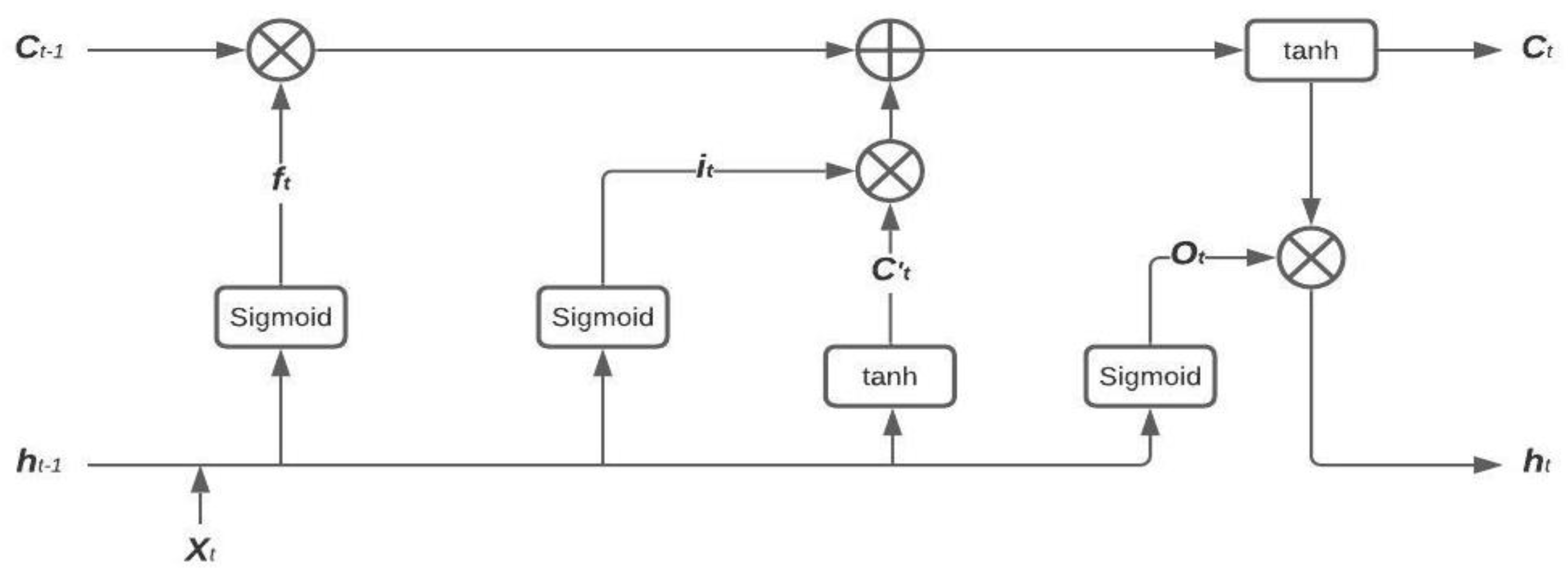
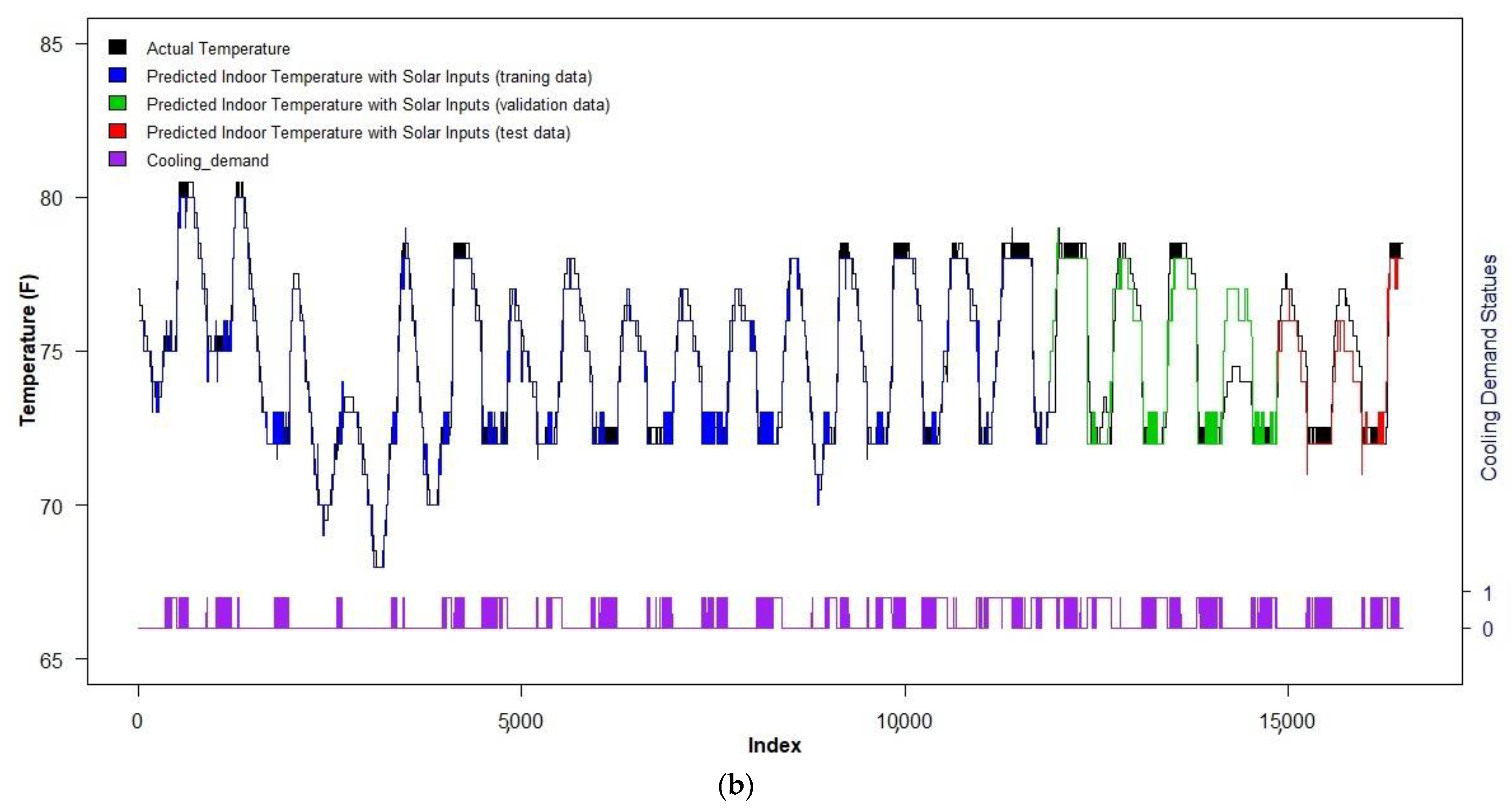
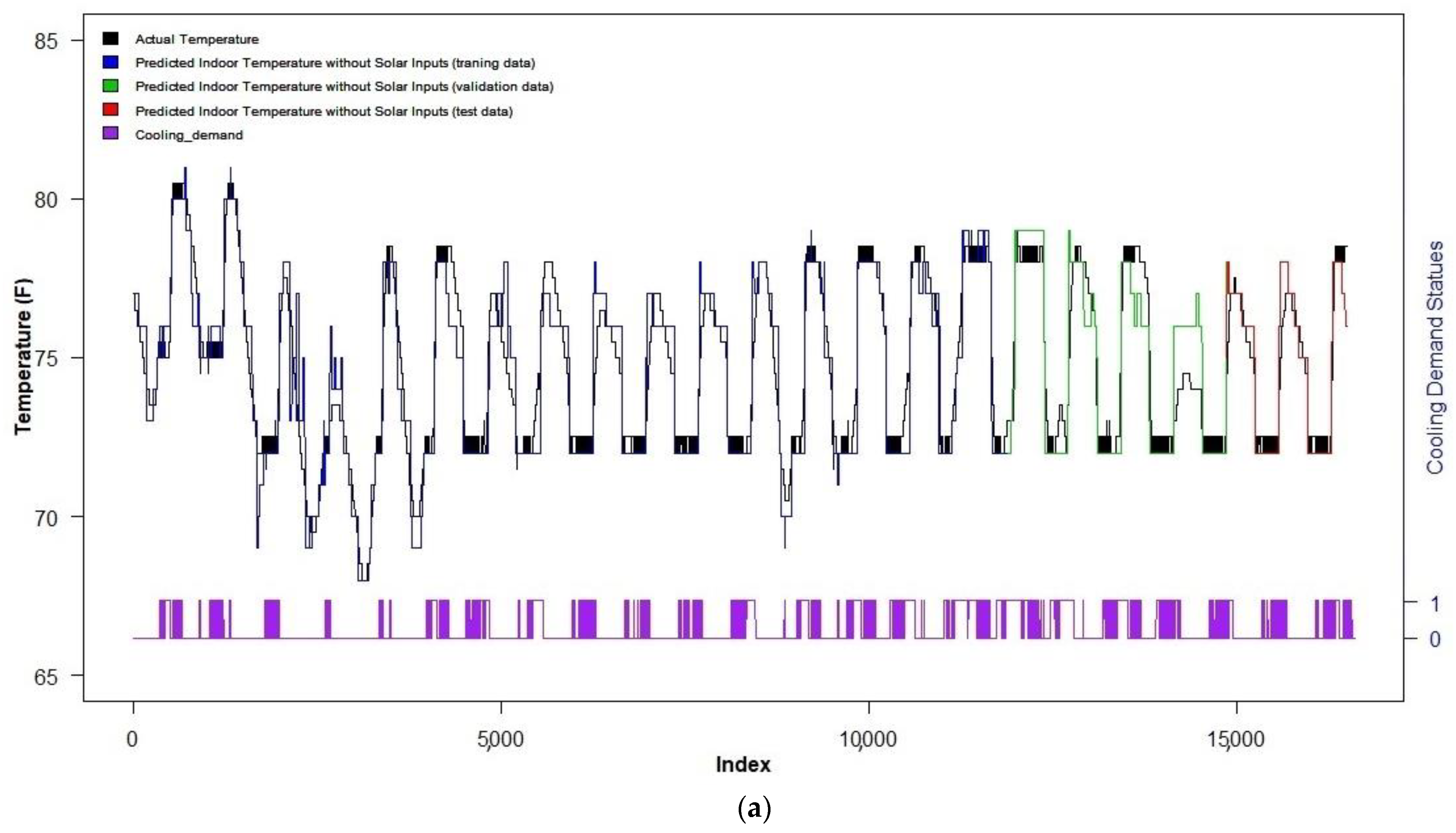
4.1.2. Model Development and Improvement

One of the aims of this research was to improve the data-enabled dynamic model to predict the indoor temperature inside a residence by accounting for solar heat gain terms. Huang et al. [27] employed various recurrent Neural Networks (RNN) described by Hochreiter and Schmidhuber in 1997 [28]. Their research showed that the Long Short-Term Memory (LSTM) algorithm yielded the most accurate predictions. The present research particularly looks to improve the LSTM model self-learning algorithm to predict indoor temperature using smart Wi-Fi thermostat and weather data through the inclusion of solar heating input data.

The Long Short-Term Memory (LSTM) neural network has a complex architecture in comparison to RNN methods, as shown in Figure 1 [28]. Basically, it has three unique gates: a forget gate (ft), which decides whether to maintain or delete the combination of the old hidden state (ht-1) and the input data (Xt); an input gate (it), which allows to new information to be stored in the cell state (Ct), and an output gate which determines the next hidden state.

The LSTM is a type of recurrent neural network (e.g., prior values of the response variable—indoor temperature—and all other inputs) can be used as predictors for the current response. The lookback period controls how far back in time prior values are used to predict the current response. Here, a lookback period of 60 points (2 h) is considered. For computational efficiency and to prevent overfitting of a model, the data is “batched”. In this study, a batch size of 128 was selected. This means that the total number of response periods was divided into 128 bins of input–output pairs. Batching enables propagation of weightings across time. This, along with regularization, helps to prevent over-fitting. Here regularization constants for L₁ and L₂ were both set to 0.0001. R-squared, MAE and RMSE metrics were employed to evaluate the validation quality.

In this study, the first 70% of the data were used for training. The remaining 30% of the data were used for testing to demonstrate confidence in the developed model to new data.

Best models were developed for input data features both including and excluding the solar input features described in Section 4.1.1.1.

4.2. Estimating Changes in Cooling Required When Solar Heating Is Included

The required cooling energy to maintain the specified thermostat setpoint temperature was calculated for the two models emerging from Section 4.1.2 (e.g., with and without solar heating inputs). This comparison permits estimation of the solar heat gain into the building and its effect on the cooling demand.

The cooling demand can be simulated through use of the developed dynamic model to predict indoor temperature using simple on–off control logic commonly used in thermostat systems. Equation (2) describes the simple control logic that was used in this research.

$$Cooling Demand Status \left(CD{S}_t\right) z=\{\begin{array}{l}ON \left(1\right), T_{indoor}>T_{cooling setpoint}+0.5°\left(F\right)\\ CD{S}_{t-1}, T_{indoor}=T_{cooling setpoint}\\ OFF \left(0\right), T_{indoor}\le T_{cooling setpoint}-0.5°\left(F\right)\end{array}$$

(2)

4.3. Estimating Impact of Solar Heat Gain on PMV Control

4.3.1. PMV Model

“Fanger’s predicted mean vote (PMV) model” is used in this study to quantify thermal comfort [13]. Its use in the literature is well documented and not described here. A seven-point thermal sensation scale proposed by the American Society of Heating, Refrigerating, and Air-Conditioning Engineers (ASHRAE) is typically used to define various levels of comfort [3]. This seven-point thermal sensation scale ranges from −3 to +3. This range accounts for the thermal comfort experienced by a majority of people. A general hot feeling corresponds to a PMV index of +3. A general cold feeling corresponds to a PMV index of −3, and so. Most people experience thermal comfort satisfaction when the PMV index ranges between −0.5 and +0.5.

The following values were set for the parameters entering into the PMV calculation. The metabolic rate, M, was set to 1 met (seated at rest), applicable to a resident sitting. The clothing insulation value, Icl, was set to 0.5 in the summer. The relative air velocity term, var, was equated to 0.1 m/s, based upon the minimum value accepted by ASHRAE-55. The room temperature and humidity were based upon the smart Wi-Fi thermostat measurement. The next section details the calculation of the MRT.

4.3.2. MRT Estimation

The mean radiant temperature (MRT) is one of the main factors needing calculation in order to quantify the thermal comfort inside a residence. Different approaches have been employed to estimate it. One of these requires direct measurement of the temperature for each interior surface in a room, and calculation of the view factors between the surfaces and a person approximated within the room [29]. However, the difficulty of identifying the angle factors due to the position of an occupant makes this approach time consuming and complex. Another effort employed use of a black-globe thermometer, along with measured room temperature and the air velocity [29]. One of the issues with this approach is the size of the black body that used in the thermometer; the smaller the size, the lower the accuracy. The simplest method equates the MRT to the indoor temperature. Collectively these approaches are either inaccurate [29] or are made impractical, through the requirement of additional measurements, beyond just the room temperature.

In a recent study, Lou et al. [12] used knowledge of the wall, window, and ceiling R-Values (information that ultimately could be inferred from smart Wi-Fi thermostat data, Alanezi et al. [21]) to develop a model to estimate the MRT which could be completely reliant upon readily available geometrical data and smart Wi-Fi thermostat data. This model estimated the interior temperature of all exterior wall and ceiling surfaces enclosing a space using smart Wi-Fi thermostat-derived envelope R-Values. To do this, a steady-state analysis with knowledge of the real-time indoor and outdoor temperature was used. Assuming negligible solar gain to an exterior surface (an assumption that will be relaxed in this study), a steady-state energy balance between the heat flow from interior surface of an envelope to the indoor air and the heat flow through the envelope component was developed. This energy balance was rearranged to obtain the interior surface temperature of envelope component according to Equation (3).

$$T_{e,in}=\frac{\left(R_e+R_{ho}\right)T_{indoor}-R_{hi}{T}_o}{R_{hi}+R_e+R_{ho}}$$

(3)

Above R_ho is the overall thermal resistance on exterior surface, R_hi is the overall thermal resistance on the interior surface (assumed to be 0.04 and 0.12 m²-K/W respectively), R_e is the conductive thermal resistance through envelope component, and T_e,in is interior surface temperature of envelope component.

Interior surfaces unconnected to exterior surfaces are assumed here to be equal to the indoor temperature, which is considered equal to the measured smart Wi-Fi thermostat temperature. Undoubtedly, there will be temperature variation within a residence. Therefore, this estimation as representative of all spaces in a residence certainly is associated with some error. However, most centrally heated and cooled residences are controlled by a single thermostat based upon temperature in a single room, so the approach posed here simply represents a natural extension of this type of whole residence HVAC control.

Solar heat gain certainly influences the thermal comfort residents perceive. Solar fenestration can cause residents to feel warmer. Moreover, solar heat gain through walls and ceilings can render warmer interior surfaces and a higher MRT. Not accounting for both in calculating the PMV, such as in the work of Lou et al. [12], as a result yields a non-conservative estimate of comfort. The following describes how the MRT model of Lou et al. was consequently modified to account for both solar heat contributions.

Exterior residential surfaces are exposed to solar irradiation during the day. This solar irradiation can be accounted for through the use of what is referred to as the sol-air temperature, T_sol-air by replacing T_o in Equation (3) with this temperature [30]. The sol-air temperature is defined by Equation (4).

$$T_{sol-air}=T_o+\frac{\alpha I_{total-solar,surface} }{h_o}-\frac{ϵ \Delta R }{h_o}$$

(4)

where I_{total-solar,surface} is the total incident solar flux exposed to a surface comprised of the diffuse, ground reflected, and beam solar irradiance, as given in Equation (1); ∆R is the difference between long wave radiation incident on surface from sky and surroundings and radiation emitted by black body at outdoor air temperature; α is the absorptance of surface for solar radiation; ϵ is the hemispherical emittance of surface, and h_o is the coefficient of heat transfer for long wave radiation and convection outer surface.

From Equations (3) and (4), the interior surface temperature of envelope component can be expressed as

$$T_{e,in}=\frac{\left(R_e+R_{ho}\right)T_{indoor}-R_{hi}{T}_{sol-air}}{R_{hi}+R_e+R_{ho}}$$

(5)

Previously, the MRT was estimated using an area weighted average of room surface temperatures as given by Equation (5). The exterior wall/ceiling component interior surface temperatures can be calculated according to Equation (6).

$$MR{T}_0=\frac{A_1{T}_{s1}+\dots +A_N{T}_{sN}}{A_1+\dots +A_N}$$

(6)

Above, the subscript 0 refers to an MRT calculation exclusive of solar fenestration. If there is solar fenestration heat gain in a room, it must influence the MRT. To compute an MRT with consideration of this, the transmitted solar heat needs to be estimated based on the incident solar irradiation to the windows, the solar incidence angle, θ_incidence, on each wall (defined as the angle between the solar irradiation on a surface and a line perpendicular to the same surface), and the solar heat gain coefficient (SHGC) as shown in Equation (7)

$$I_{transmitted-solar,window,i}=I_{total-solar}*SHGC \left({\theta }_{incidence,i}\right)$$

(7)

where i represents the ith surface.

With the transmitted solar radiation through fenestration on each surface, a delta MRT for each room can be calculated using an average transmitted solar energy from multiple windows in a space (Equation (7)) from Equation (8) [29,30].

$$I_{transmitted-solar}=I_{transmitted-solar,window,i}+\dots +I_{transmitted-solar,window,n}$$

(8)

where n is the number of surfaces in a room which allow solar radiation to be transmitted through fenestration.

The effect of solar fenestration on human feeling of comfort can be accounted for through use of a radiation heat transfer coefficient acting between the actual mean radiant temperature and the indoor temperature as referenced in ASHRAE 55 [30], according to:

$$Q_{rad}=I_{transmitted-solar}=h_r \left(MR{T}_{actual}-T_{indoor}\right)$$

(9)

Here, $MR{T}_{actual}=MR{T}_0+\Delta MRT$, where $\Delta MRT$ is the change in MRT as a result of solar fenestration. The radiation heat transfer coefficient in the standard is listed at typically being 4.7 W/m²-K [29].

As a first approximation, T_indoor can be equated to $MR{T}_0$. This assumption is reasonable when solar fenestration gain has a small effect on MRT (if the window area is small relative to the wall area) and when the walls and ceiling are reasonably well insulated. All residences in this study had window area fractions of no more than 0.14 so the first requirement is satisfied. However, the latter is only satisfied in the higher efficiency residences considered here. With this assumption, Equation (10) can be reorganized to solve for $\Delta MRT$ acording to:

$$\Delta MRT=\frac{I_{transmitted-solar}}{h_r}$$

(10)

The actual MRT can then be approximated as:

$$MR{T}_{actual}~MRT+\Delta MRT$$

(11)

4.3.3. Summary of PMV Calculations

While these values have been set, they are offered with caution. A recent review of fifty years of the PMV model acknowledges that improper specification of any of these parameters can significantly affect the PMV calculation. The EN 16798-1 and 16798-2 Standards offer guidance about how all six terms in the PMV can be calculated, but doing so in practice can be difficult [31]. The methodology posed here leverages reasonable values for the terms which are not measured and for the PMV. The thermal comfort savings calculated will therefore nominal. However, the actual thermal comfort for a residence ultimately could adapt to resident feedback of discomfort when the algorithm is not working for the residents. This type of feedback would improve the resident specific model of thermal comfort.

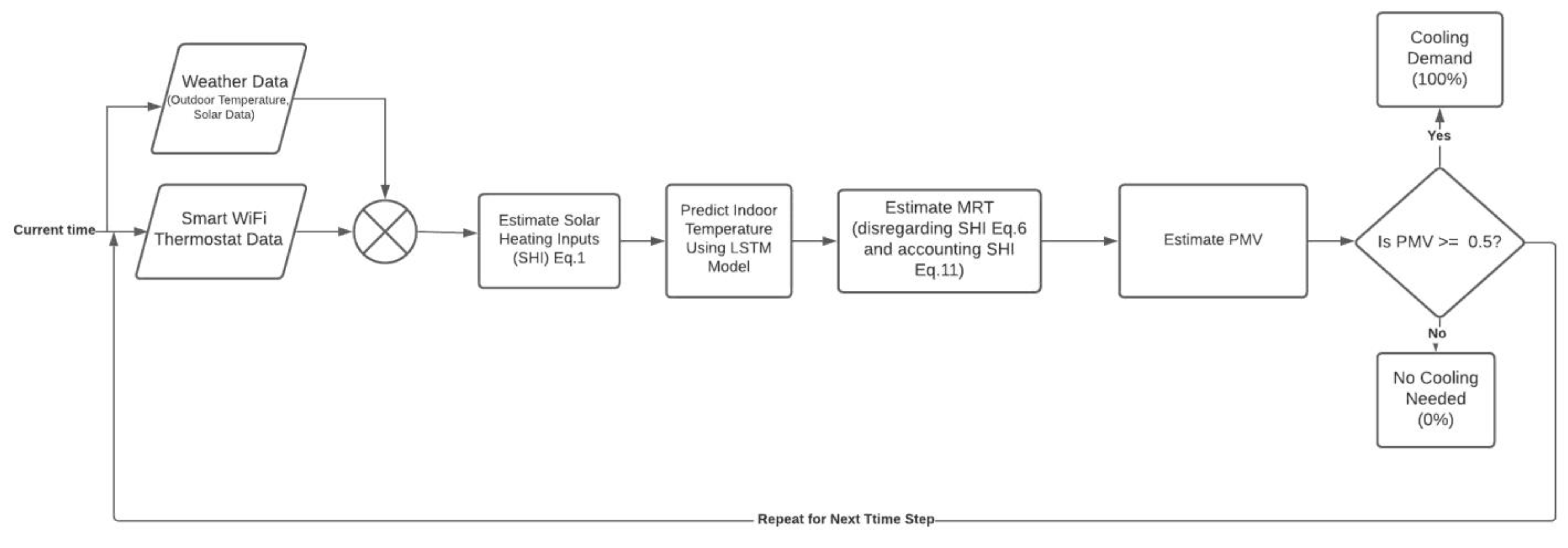
4.3.4. Thermal Comfort Control Logic

A simple on–off control logic based upon measuring the internal temperature and humidity, estimating the current PMV values, and comparing the present value to the desired or setpoint PMV value was employed. This comparison will then prompt the turning on or off the HVAC system. Here the PMV setpoint was 0.25 (slightly warm). A +− PMV setpoint delta of 0.25 was established. Thus, if the PMV value rose above 0.5, cooling was initiated. If it fell below 0, cooling was disengaged. Otherwise, the cooling demand was not changed from the prior state.

The flowchart shown in Figure 2 summarizes the complete control strategy. In step 1, current weather data are accessed and synchronized with the smart Wi-Fi data. The next step is to estimate the solar heat inputs using Equation (1) mentioned previously in Section 2 to identify their effect on thermal comfort. Next the indoor temperature is predicted using the trained LSTM Model obtained from historical weather data, smart Wi-Fi data, and solar related data (described in Section 4.1.2). The subsequent step is to estimate for a given zone the MRT; in one case, disregarding solar heating inputs, as given by Equation (6), and in other case, accounting for solar heating inputs, as given by Equation (11). With an MRT calculated, the PMV index can be determined at each sampled time considering the predicted indoor temperature, the indoor humidity obtained from thermostat data, estimated mean radiant temperature (MRT), and occupants’ data (M ranges from 1.1–1.3 met and I_cl ranges from 0.36–0.5 clo). The last step is to check if the estimated PMV value is larger or equal to the highest desired PMV value; if the PMV value is larger or equal to 0.5, the cooling demand is set to 100%; if it is below 0, the cooling demand is set to 0%; otherwise, it is not changed. This control logic is repeated each time step in this study.

4.4. Evaluating Savings from PMV Control with Solar Contributions Accounted For

As was reviewed in Section 2, energy savings from thermal comfort control, not temperature control, have been reported as ranging from 10–85% depending on several factors, such as location of the building, the number of the occupants, and other factors related to the PMV. Comparing savings from thermal comfort control to conventional controls, it can be seen clearly that utilizing comfort controls would have an impact on the global energy reduction goals as well as carbon dioxide pollution. The prior work of Lou et al. reported savings at the high end of this range. However, as previously mentioned, their work did not consider solar heat gain contributions to comfort.

Here we estimate cooling energy savings from thermal comfort control for the five residences shown in Table 2 for the time period from 2/6/2018–24/6/2018 for actual weather conditions and with and without consideration of solar heat gain. The baseline for comparison is a temperature control scenario, where the indoor setpoint temperature was considered to be 22 °C during the day (from 6 a.m.–5 p.m.) and 26 °C during the remainder of the day.

The cooling energy consumption was determined by considering the cooling size of the residence’s HVAC and the effective duty cycle for the whole period. The cooling duty cycle is defined as:

$$Effective Duty Cycle=\frac{{\displaystyle \sum }\left(Cooling time\right)\times \left(Cooling Demand Status\right)}{{\displaystyle \sum }Time}$$

(12)

5. Results

LSTM machine learning predictive models for the residential internal temperature were developed using the input features previously described in Section 4.1.1.2. Best models were developed with and without inclusion of the solar input terms. As noted previously, the models were trained using the earliest 70% of the data. The remainder of the data was used for testing.

Table 5. Hyper-parameter settings and validation metrics for the best model developed for each consideration.

Model	Lookback Steps	Hidden Layers (Units)			Batch Size	MAE	R2	MAPE (%)	RMSE
LSTM w/o Solar Inputs	30	40	25	15	128	0.66296	0.847	0.866	1.003
LSTM w/Solar Inputs	30	40	25	15	128	0.406	0.912	0.537	0.627

shows the hyper-parameter settings and validation metrics for both considerations (disregarding and accounting for solar inputs).

Figure 3a shows a time series plot of the measured indoor temperature and the predicted indoor temperature over the entire time period without taking solar heating inputs into account for House #1 (with almost 50% shading and medium insulation level). Figure 3b shows a similar plot for the model including solar heating inputs. A comparison between the two plots, especially in the validation and testing range, shows a substantial improvement in the predictions. This same result was seen for all of the residences considered. Clearly the additional solar heat inputs are critical for improvement of the predictive model in comparison the results of Lu et al., which was effectively represented by the case shown in Figure 3a.

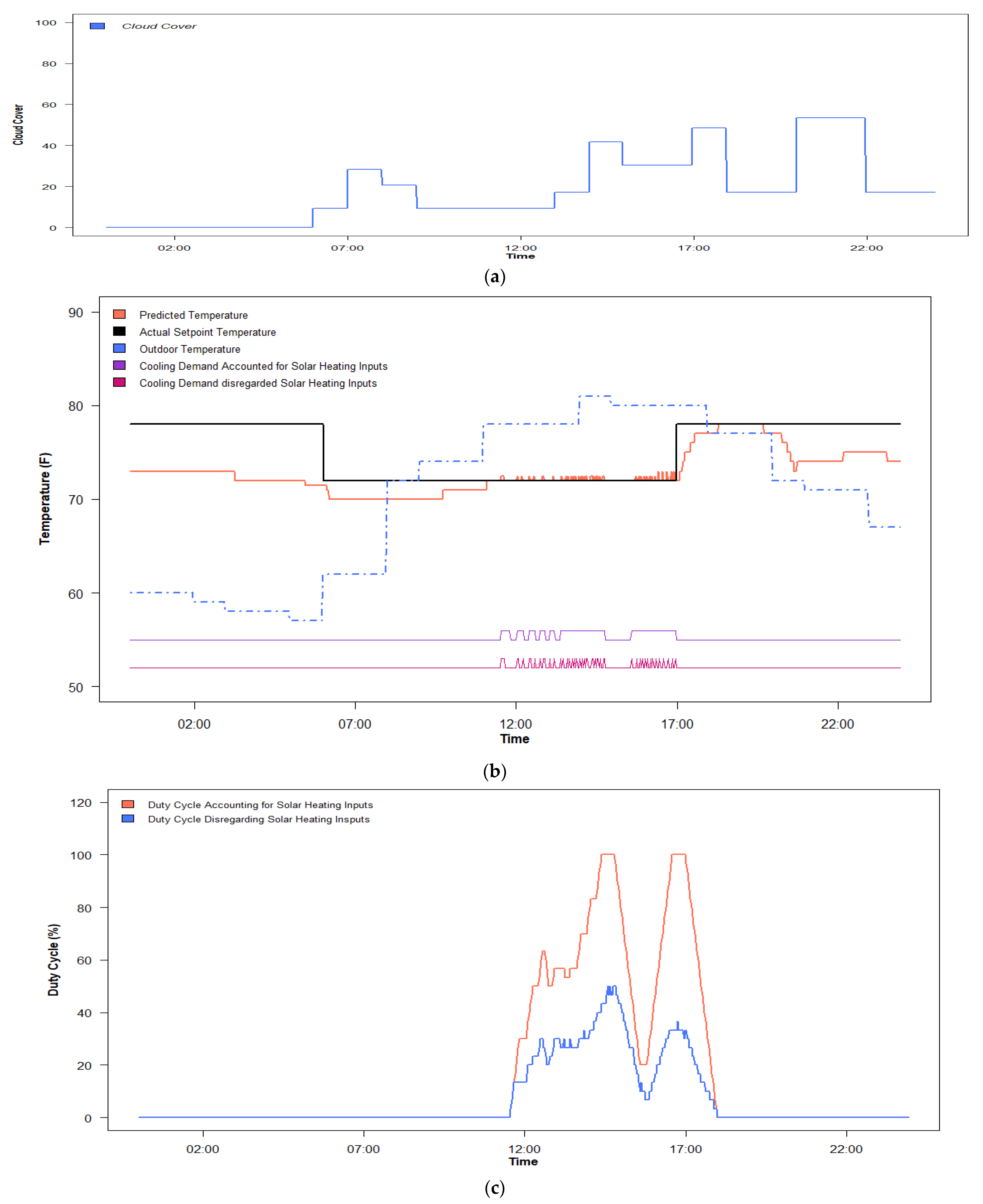
5.1. Cooling Reduction from Thermal Comfort Control versus Traditional Temperature Control with and without Consideration of Solar Heat Gain

Solar heat gain certainly increases the required cooling of a residence. Figure 4 shows a time series for a fairly cloudy day (Figure 4a) of the predicted temperature, actual setpoint temperature, and predicted real time cooling demand with and without inclusion of the solar heat input terms (Figure 4b). Figure 4c shows the cooling duty cycle for a 24 h window for the solar heat input and no solar heat input cases. It is obvious that the required cooling is slightly reduced due to the high cloud cover during the day. It can be inferred that solar heat gain effects on the cooling required to maintain comfort are relatively small.

Figure 5 shows similar results for a mostly sunny day. It is clear especially from comparison of the cooling duty cycle with and without solar terms of Figure 5c to Figure 4c that this reveals a much greater reduction in cooling if solar inputs are not considered for the sunny day case. Solar heating in the cloudy case accounts for 17% of the cooling, whereas in the mostly sunny case, it accounts for 58%.

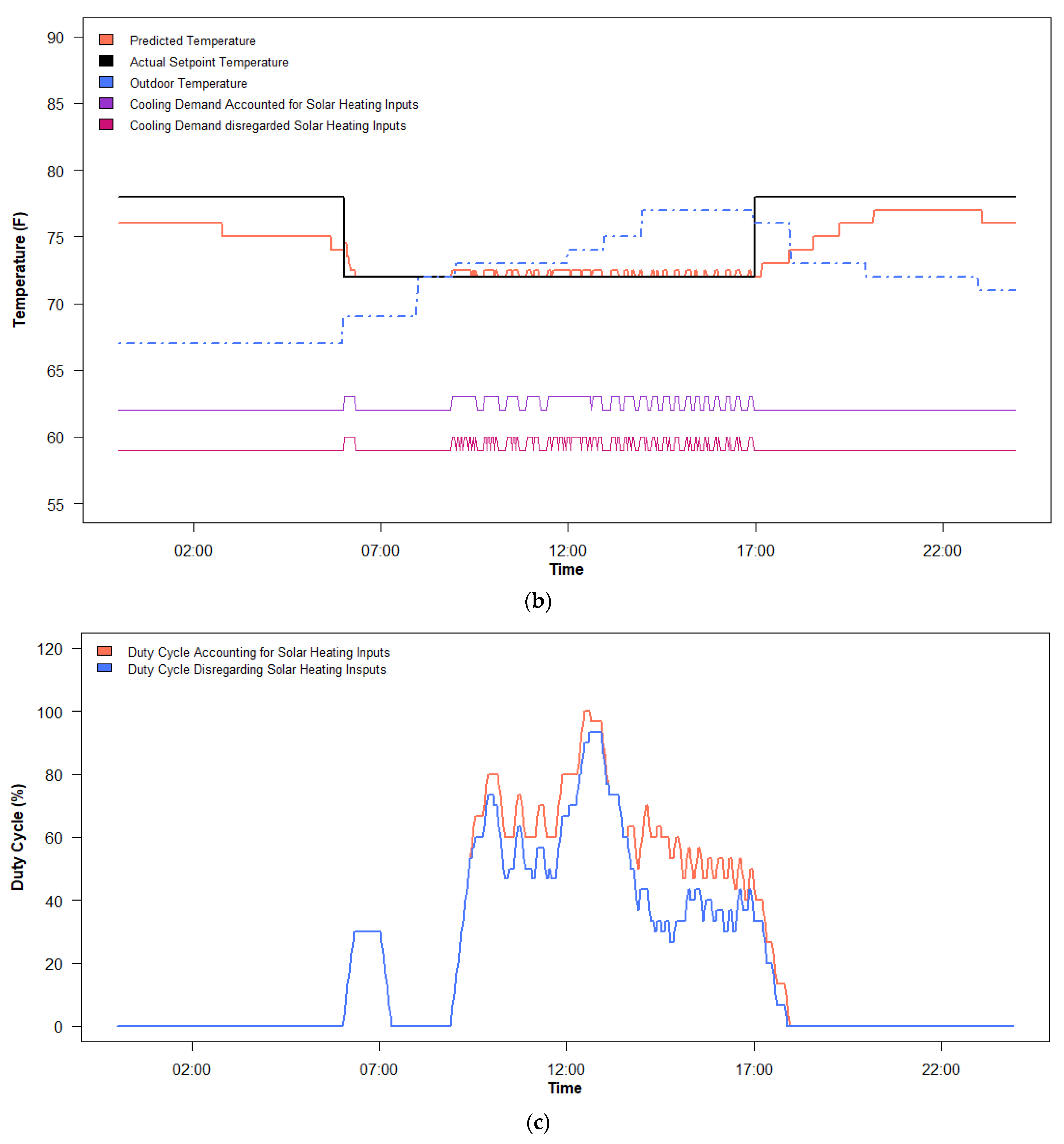
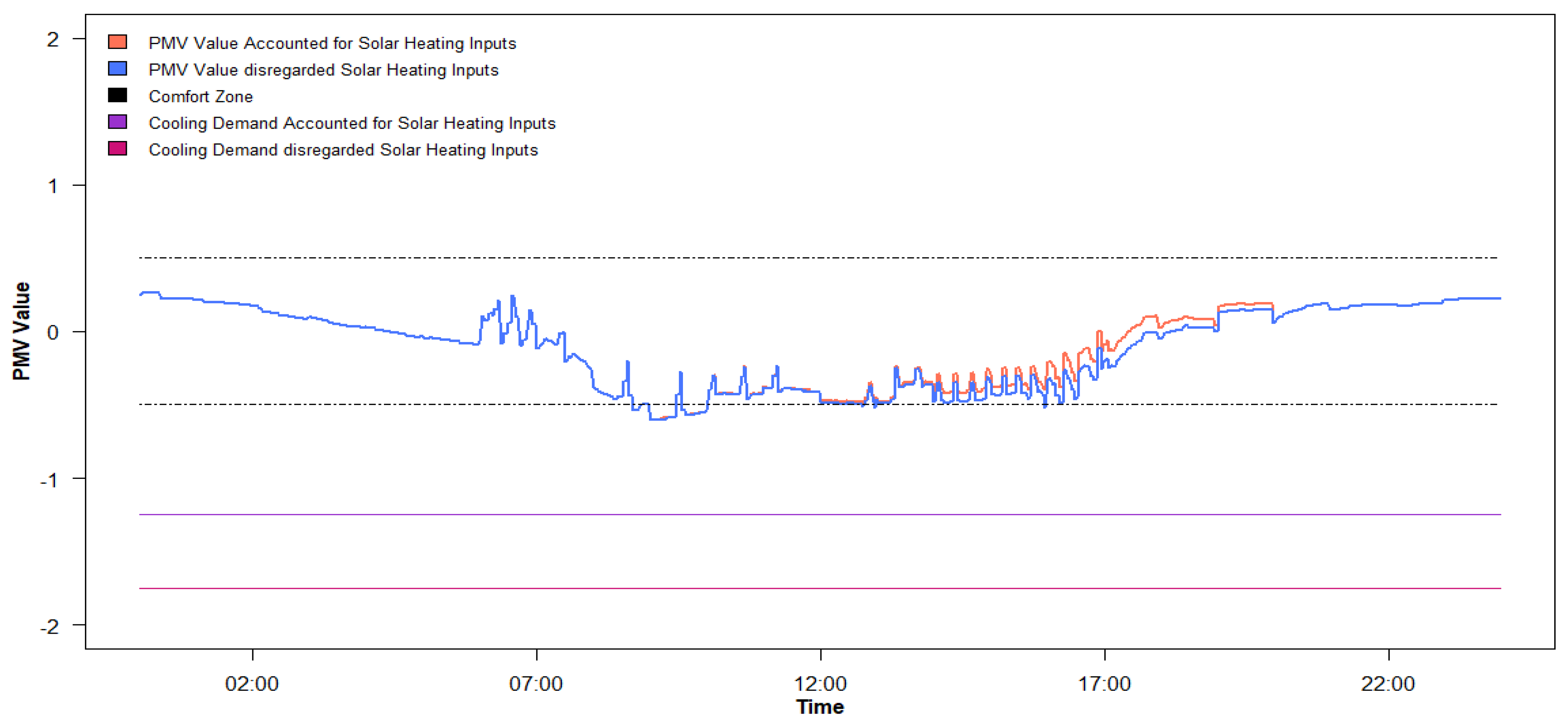
5.2. Impact of Solar Heat Gain on PMV Value

Figure 6 and Figure 7 provides time series of the PMV values calculated for the cases considered in Figure 4 (mostly cloudy) and Figure 5 (mostly sunny) with and without consideration of solar heating. The two plots reveal the impact of the solar heat gain on the actual PMV for, respectively, a mostly cloudy and mostly sunny day for the same residence. It is clear for the mostly cloudy case presented in Figure 6 that the solar heat gain has little impact on the actual PMV value. In contrast, Figure 7 reveals a large difference between the PMV value calculated by accounting for solar heat gain and discounting it. The solar heat gain case yields a substantially higher PMV value.

5.3. Savings from PMV Control with Solar Heat Gain Contributions Accounted For

Figure 8 shows a comparison of the total cooling energy consumption for several residences over the complete time period for three cases: (i) the actual temperature control case (baseline); (ii) thermal comfort control with solar heat gain contributions considered, and (iii) thermal comfort control when solar heat gain contributions were not considered. The light blue bars represent the actual cooling energy consumption, while the red and the dark blue bars represent the cooling energy consumption for thermal comfort with and without considering solar heat gain. PMV control simulations were conducted for each of the residences shown in Figure 2 in order to evaluate the impact of residence shading.

From this figure it is clear that for all residences, inclusion of the solar heat gain contributions yields smaller savings from PMV-based thermal comfort control than similar calculations if these contributions are not included. This result is not surprising. However, this research uniquely uses actual data and a well-validated model to demonstrate this. It also shows that the amount of savings depends upon the amount of shading a residence has. With greater shading (e.g., Houses 2 and 4), smaller differences in savings from PMV-based thermal comfort control between the solar heat gain and non-solar heat gain cases are estimated in comparison to residences with less shading (e.g., Houses 1, 3, and 5). It is also clear that residences with greater wall and ceiling insulation see smaller savings from thermal comfort control (House 4 is the most insulated house). In contrast, the residence having the poorest insulation is associated with the biggest savings from thermal comfort control (House 2 and 3).

Table 6. Savings from application of thermal comfort control logic for the residences considered in study.

	House #1	House #2	House #3	House #4	House #5
Insulation Level	Medium	Low	Low	High	Medium
Savings from Thermal Comfort Control w/ and w/out Solar Heat Gain Consideration	40%/53%	47%/56%	46%/60%	33%/43%	40%/52%

summarizes the savings from thermal comfort control for each of the residences included in this study and for both the solar heat gain contribution and non-solar heat gain cases.

In this study, cooling energy savings range from 33 to 47% by applying thermal comfort control with consideration of solar heat gain, well below that observed by Lou et al. [13], whereas cooling energy savings range from 43 to 60% if solar heat gain is not considered.

6. Conclusions

This paper has demonstrated improvement in data-based machine learning dynamic models to predict the indoor temperature through the addition of solar heating inputs. Model improvements were made possible through the use of an LSTM algorithm and through accounting of solar heat gain. This model was critical to the conduct of what-if assessments which permitted both improved accuracy of cooling energy savings from thermal comfort control and quantitative estimation of the solar heat gain contribution to any residence. In total, cooling energy savings from thermal comfort when considering more realistic solar heat gain ranged from 33 to 47%; in contrast, 43 to 60% were solar heat gain to be ignored. The extent of savings and the influence of solar heat gain on it was seen to depend upon the energy effectiveness of a residential construction and the level of shading. Greater wall and ceiling insulation reduces thermal comfort savings potential.

The value of this research is that is shows that smart Wi-Fi thermostat data in any residence can be used to estimate thermal comfort control energy savings. Such information should be extremely useful for policy makers and smart Wi-Fi thermostat manufacturers.

It is clear that there are limitations of this research. The modified MRT approach used here relies upon knowledge of the number and type of windows in a room. This information would certainly be difficult to come by. There is a potential work-around relative to this issue; however, one that is enlightened by the research posed here. The difference in cooling required with and without solar heat gain should permit estimation of solar heat gain to the residence. This data-based assessment, derived from models developed with and without solar contributions, could be performed readily for any residence using smart Wi-Fi thermostat data. A corrected MRT could be developed from this solar heat gain estimate. Further, the corrected MRT calculation should be validated with measurements.

Secondly, while the savings estimations were reasonable and saw expected dependency on residence efficiency and solar heat gain, there is a need to validate the estimations. There is a need to implement this strategy in multiple residences and validate resident perceived thermal comfort. The implementation must include resident feedback about when the algorithm is not providing them the thermal comfort they desire. The thermal comfort model would then need to adapt based upon this feedback.

More importantly, in order to derive value from this research, it is essential that a smart Wi-Fi thermostat manufacturer integrate this technology into their thermostat control algorithms. This will also require such manufacturers to market and sell comfort control to its customers.

There is a wealth of future research potentially triggerable by this research. Here, as noted above, the corrected MRT was obtained based upon estimation of the solar fenestration. This approach could be very laborious if it was implemented at scale. It is feasible that Geographical Information Systems (GIS) could be used to automatically make this calculation for any residence using technologies such as Google Earth. Secondly, there is opportunity for research to estimate aggregate potential savings from regional efforts to improve shading and to implement thermal comfort control.

References

1. Masson-Delmotte, V.; Zhai, P.; Pörtner, H.-O.; Roberts, D.; Skea, J.; Shukla, P.R.; Pirani, A.; Moufouma-Okia, W.; Péan, C.; Pidcock, R. (Eds.) IPCC, 2018: Global Warming of 1.5 °C. An IPCC Special Report on the Impacts of Global Warming of 1.5 °C above Pre-Industrial Levels and Related Global Greenhouse Gas Emission Pathways, in the Context of Strengthening the Global Response to the Threat of Climate Change, Sustainable Development, and Efforts to Eradicate Poverty; in press; IPCC: Geneva, Switzerland, 2018. [Google Scholar]
2. Stanford University Energy and Climate Plan. Available online: https://sustainable.stanford.edu/sites/default/files/E%26C%20Plan%202016.6.7.pdf (accessed on 26 June 2021).
3. Hand, M.M.; Baldwin, S.; DeMeo, E.; Reilly, J.M.; Mai, T.; Arent, D.; Porro, G.; Meshek, M.; Sandor, D. (Eds.) Renewable Electricity Futures Study (Entire Report) National Renewable Energy Laboratory. Renewable Electricity Futures Study; NREL/TP-6A20-52409; National Renewable Energy Laboratory: Golden, CO, USA, 2012. Available online: http://www.nrel.gov/analysis/re_futures/ (accessed on 13 April 2021).
4. Puget Sound Energy: Major HVAC Controls Upgrade Rebates. PSE. Available online: https://www.pse.com/en/business-incentives/commercial-hvac-upgrade-incentives/major-hvac-controls-upgrade-rebates (accessed on 13 April 2021).
5. Masoso, O.; Grobler, L.J. The dark side of occupants’ behaviour on building energy use. Energy Build. 2010, 42, 173–177. [Google Scholar] [CrossRef]
6. Vakiloroaya, V.; Samali, B.; Fakhar, A.; Pishghadam, K. A review of different strategies for HVAC energy saving. Energy Convers. Manag. 2014, 77, 738–754. [Google Scholar] [CrossRef]
7. Ghahramani, A.; Dutta, K.; Yang, Z.; Ozcelik, G.; Becerik-Gerber, B. Quantifying the influence of temperature setpoints, building and system features on energy consumption. In Proceedings of the Winter Simulation Conference (WSC); Huntington Beach, CA, USA, 6–9 December 2015, IEEE: Piscataway, NJ, USA, 2015; pp. 1000–1011. [Google Scholar]
8. Ghahramani, A.; Dutta, K.B. Becerik-gerber, energy trade off analysis of optimized daily temperature setpoints. J. Build. Eng. 2018, 19, 584–591. [Google Scholar] [CrossRef]
9. Kaam, S.; Raftery, P.; Cheng, H.; Paliaga, G. Time-averaged ventilation for optimized control of variable-air-volume systems. Energy Build. 2017, 139, 465–475. [Google Scholar] [CrossRef] [Green Version]
10. Yang, L.; Yan, H.; Lok, C. Thermal comfort and building energy consumption implications—A review. Appl. Energy 2014, 115, 164–173. [Google Scholar] [CrossRef]
11. Park, J.; Kim, T.; Lee, C. Development of Thermal Comfort-Based Controller and Potential Reduction of the Cooling Energy Consumption of a Residential Building in Kuwait. Energies 2019, 12, 3348. [Google Scholar] [CrossRef] [Green Version]
12. Lou, R.; Hallinan, K.; Huang, K.; Reissman, T. Smart Wifi Thermostat-Enabled Thermal Comfort Control in Residences. Sustainability 2020, 12, 1919. [Google Scholar] [CrossRef] [Green Version]
13. Fanger, P.O. Thermal Comfort: Analysis and Applications in Environmental Engineering; McGraw-Hill: New York, NY, USA, 1970. [Google Scholar]
14. Khovalyg, D.; Kazanci, O.; Gundlach, I.; Bahnfleth, W.; Toftum, J.; Olesen, B.W. Impact of Indoor Environmental Quality Standards on the Simulated Energy Use of Classrooms. In Proceedings of the Windsor Conference 2020, Windsor, UK, 16–19 April 2020. [Google Scholar]
15. Azuatalam, D.; Lee, W.; de Nijs, F.; Liebman, A. Reinforcement Learning for Whole-building HVAC Control and Demand Response. Energy AI 2020, 2, 100020. [Google Scholar] [CrossRef]
16. Li, Y.; de la Ree, J.; Gong, Y. The Smart Thermostat of HVAC Systems Based on PMV-PPD Model for Energy Efficiency and Demand Response. In Proceedings of the 2018 2nd IEEE Conference on Energy Internet and Energy System Integration (EI2), Beijing, China, 20–22 October 2018; pp. 1–6. [Google Scholar] [CrossRef]
17. Deng, Z.; Chen, Q. Artificial neural network models using thermal sensations and occupants’ behavior for predicting thermal comfort. Energy Build. 2018, 174, 587–602. [Google Scholar] [CrossRef]
18. Chemingui, Y.; Gastli, A.; Ellabban, O. Reinforcement Learning-Based School Energy Management System. Energies 2020, 13, 6354. [Google Scholar] [CrossRef]
19. Hong, S.; Lee, J.; Moon, J.; Lee, K. Thermal Comfort, Energy and Cost Impacts of PMV Control Considering Individual Metabolic Rate Variations in Residential Building. Energies 2018, 11, 1767. [Google Scholar] [CrossRef] [Green Version]
20. Smart Thermostat Market. Market Research Firm. Available online: https://www.marketsandmarkets.com/Market-Reports/smart-thermostat-market-266618794.html (accessed on 15 April 2021).
21. Alanezi, A.M.; Hallinan, K.; Huang, K. Automated Residential Energy Audits Using a Smart WiFi Thermostat-Enabled Data Mining Approach. Energies 2021, 14, 2500. [Google Scholar] [CrossRef]
22. Altarhuni, B.; Naji, A.; Brodrick, P.; Hallinan, K.; Brecha, R.J.; Yao, Z. Large scale residential energy efficiency prioritization enabled by machine learning. Energy Efficiency 2019, 12, 2055–2078. [Google Scholar] [CrossRef]
23. Responsible Party DOC/NOAA/NESDIS/NCEI. National Centers for Environmental Information, NESDIS, NOAA, U.S. Department of Commerce (Point of Contact). NOAA’s Climate Divisional Database (nCLIMDIV). NOAA’s Climate Divisional Database (nCLIMDIV)—CKAN. Available online: https://catalog.data.gov/dataset/noaas-climate-divisional-database-nclimdiv (accessed on 10 January 2021).
24. NASA. Prediction of Worldwide Energy Resources (Power). (2020, November 12). Available online: https://catalog.data.gov/dataset/prediction-of-worldwide-energy-resources-power (accessed on 24 March 2021).
25. Duffie, J. Solar Engineering of Thermal Processes; John Wiley: Hoboken, NJ, USA, 2020. [Google Scholar]
26. Xu, P.; Han, S.; Huang, H.; Qin, H. Redundant features removal for unsupervised spectral feature selection algorithms: An empirical study based on nonparametric sparse feature graph. Int. J. Data Sci. Anal. 2018, 8, 77–93. [Google Scholar] [CrossRef]
27. Huang, K.; Hallinan, K.; Lou, R.; Alanezi, A.M.; Alshatshati, S. Sun, Q. Self-Learning Algorithm to Predict Indoor Temperature and Cooling Demand from Smart WiFi Thermostat in a Residential Building. Sustainability 2020, 12, 3685. [Google Scholar]
28. Sepp, H.; Schmidhuber, J. Long Short-Term Memory. Neural Comput. 1997, 9, 1735–1780. [Google Scholar] [CrossRef]
29. AHSRAE. ASHRAE Handbook—Fundamentals; ASHRAE, Inc.: Atlanta, GA, USA, 2005. [Google Scholar]
30. Arens, E.; Hoyt, T.; Zhou, X.; Huang, L.; Zhang, H.; Schiavon, S. Modeling the comfort effects of short-wave solar radiation indoors. Build. Environ. 2015, 88, 3–9. [Google Scholar] [CrossRef] [Green Version]
31. d’Ambrosio Alfano, F.R.; Olesen, B.W.; Palella, B.I.; Pepe, D.; Riccio, G. Fifty Years of PMV Model: Reliability, Implementation and Design of Software for Its Calculation. Atmosphere 2020, 11, 49. [Google Scholar] [CrossRef] [Green Version]
Figure 1. Long Short term memory architecture.
Cleantechnol 03 00044 g001
Figure 2. Flowchart showing process for simulated thermal comfort control using developed LSTM Deep Learning Neural Network model of internal temperature.
Cleantechnol 03 00044 g002
Figure 3. Actual temperature versus predicted temperature using whole dataset using an LSTM model for these cases: (a) without consideration of solar heating inputs and (b) with consideration solar heating inputs.
Cleantechnol 03 00044 g003aCleantechnol 03 00044 g003b
Figure 4. Time series plots for a mostly cloudy day for: (a) cloud cover; (b) predicted temperature and cooling requirements (with and without solar heat inputs) for given outdoor temperature and indoor temperature setpoint variation, and (c) cooling duty cycle for 24 h time window with and without solar heating inputs.
Cleantechnol 03 00044 g004aCleantechnol 03 00044 g004b
Figure 5. Time series plots for a mostly sunny day for the same residence shown in Figure 4 for (a) cloud cover; (b) predicted temperature and cooling requirements (with and without solar heat inputs) for given outdoor temperature and indoor temperature setpoint variation, and (c) cooling duty cycle for 24 h time window with and without solar heating inputs.
Cleantechnol 03 00044 g005
Figure 6. Time series plots of real time PMV value and cooling demand for the solar heat gain and non-solar heat gain cases.
Cleantechnol 03 00044 g006
Figure 7. Time series plots of real time PMV value and cooling demand for the solar heat gain and non-solar heat gain cases.
Cleantechnol 03 00044 g007
Figure 8. Comparative cooling energy consumption for residences included in Table 2 for three cases: (1) actual, (2) PMV control with solar heat gain, and (3) PMV control without solar heat gain.
Cleantechnol 03 00044 g008