
Kalman Filter-Based Real-Time Implementable Optimization of the Fuel Efficiency of Solid Oxide Fuel Cells


Abstract
1. Introduction
2. Modeling of the Electric Power Characteristic of Solid Oxide Fuel Cells
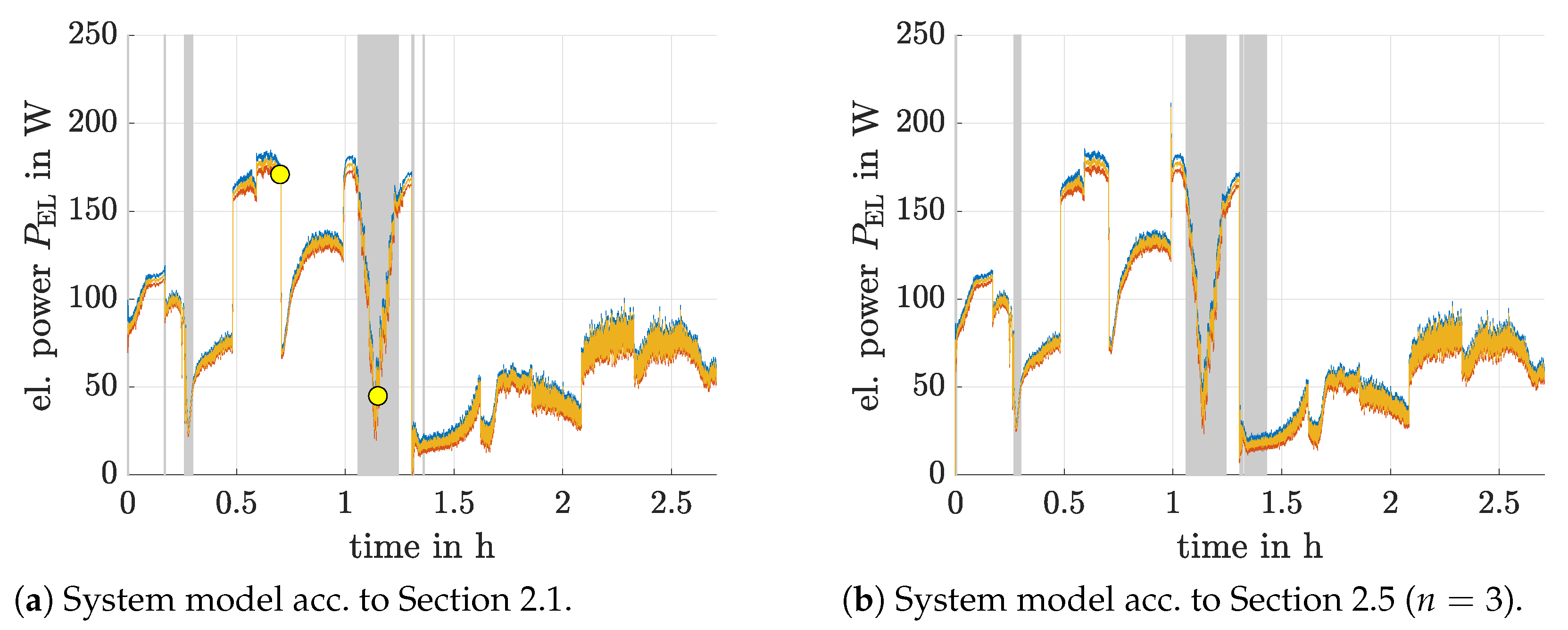
2.1. Static Neural Network Model
2.2. Optimization of the Neural Network Structure
2.2.1. Optimal Network Inputs
2.2.2. Optimal Number of Hidden Layer Neurons
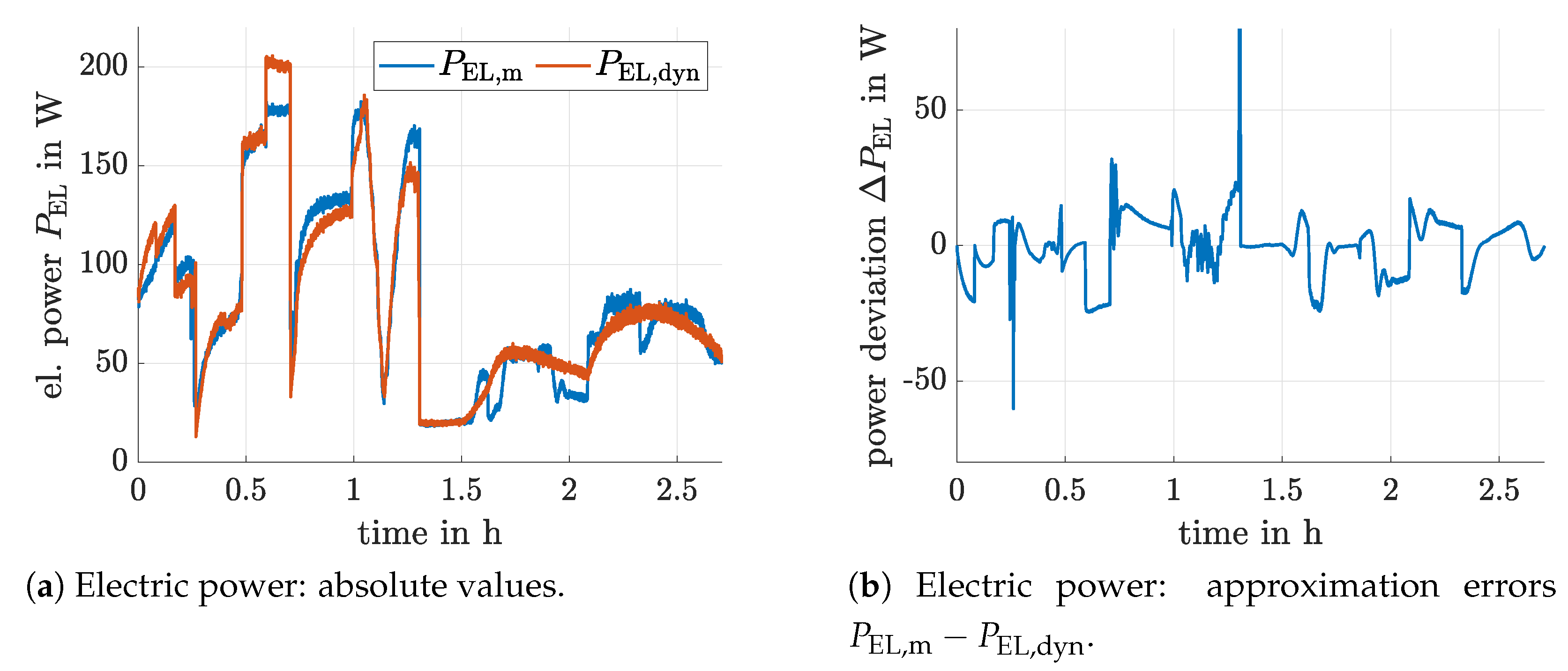
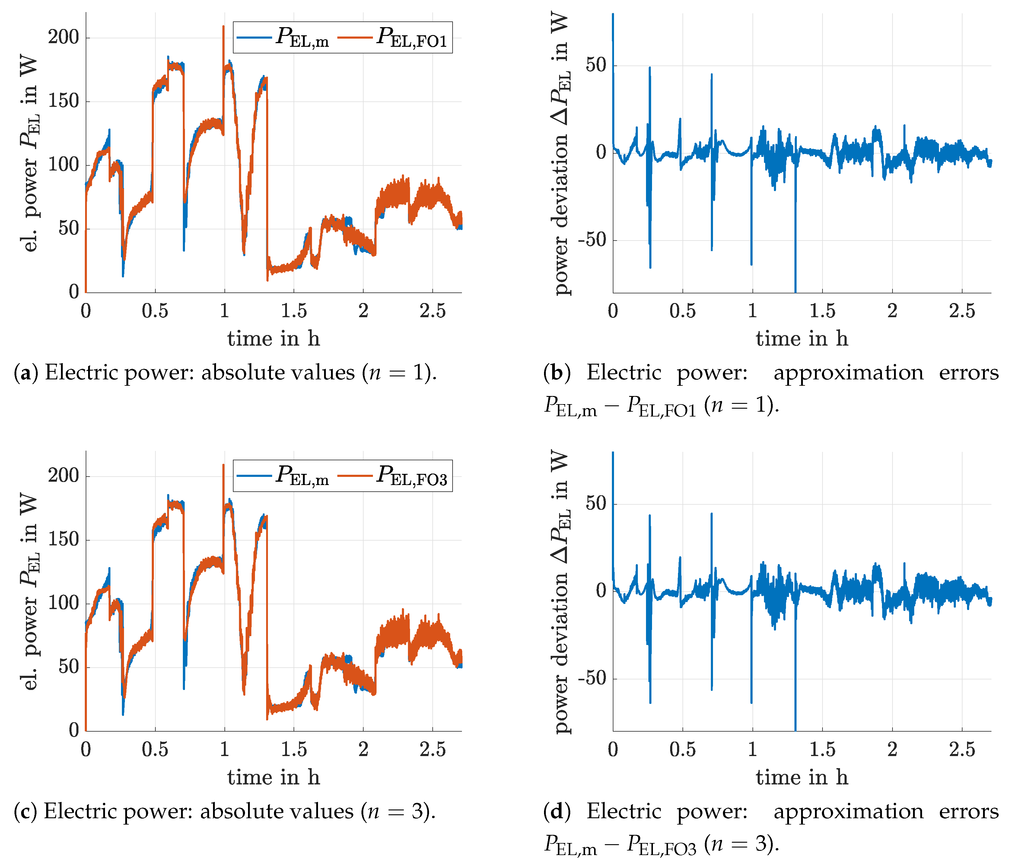
2.3. First-Order Dynamic Neural Network Model
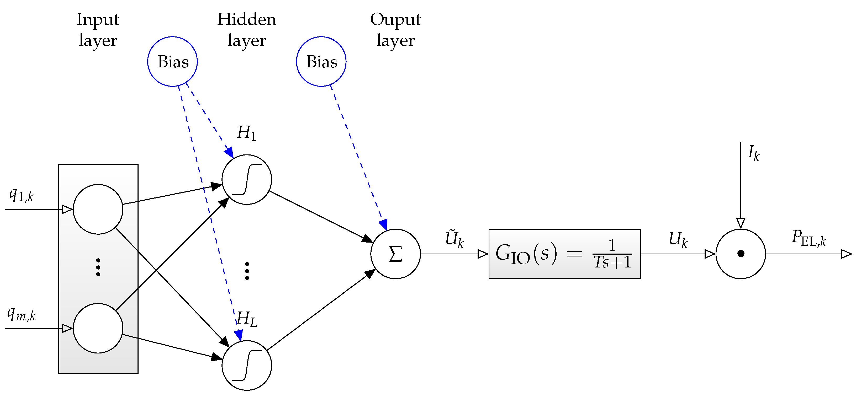
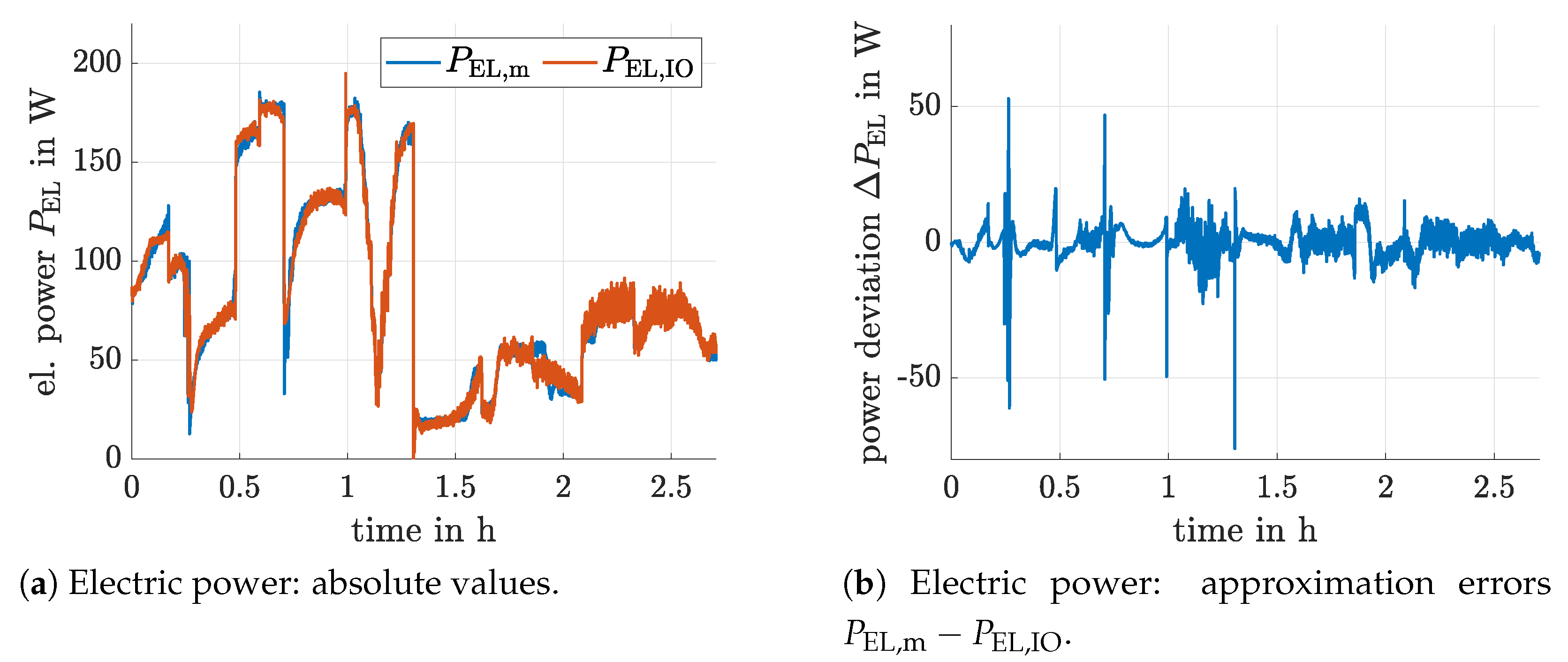
2.4. Hammerstein Neural Network Model with Integer-Order Dynamics
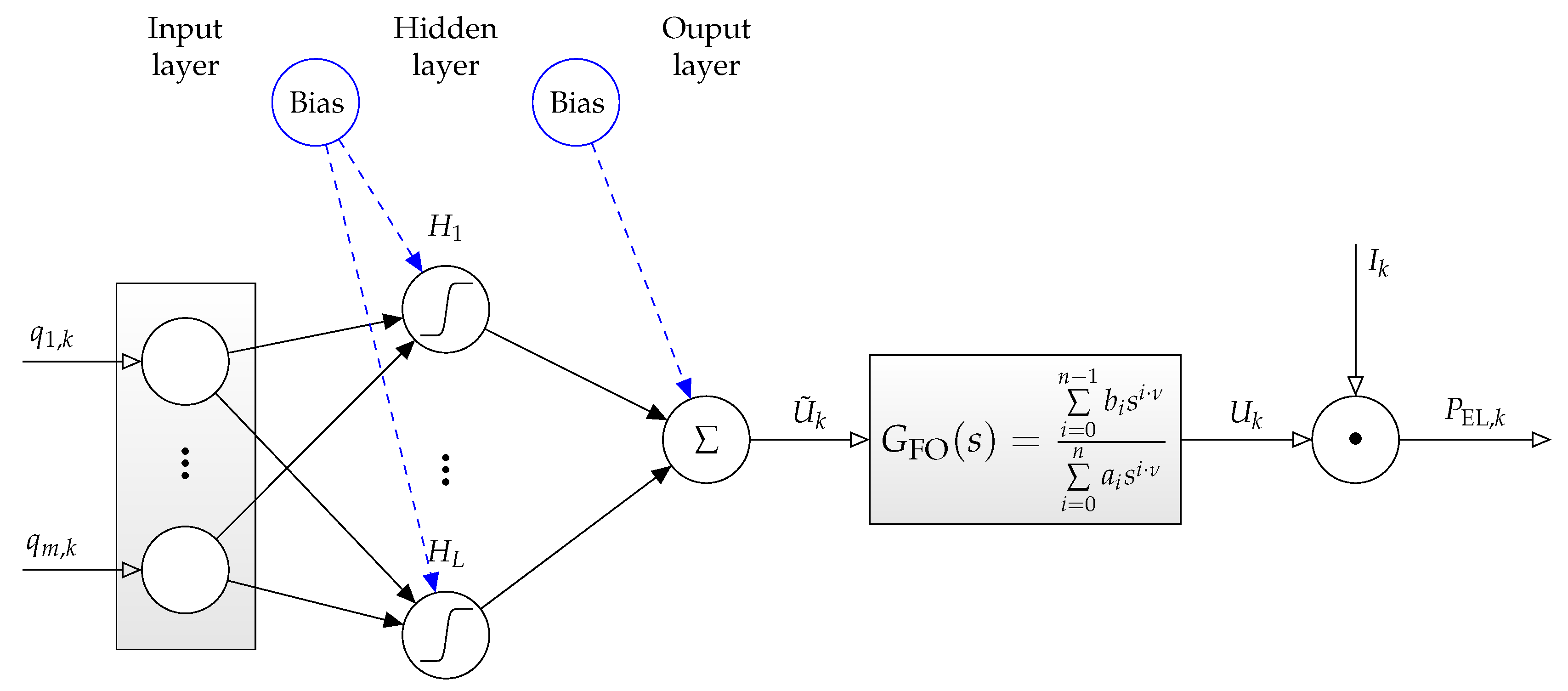
2.5. Hammerstein Neural Network Model with Fractional-Order Dynamics
3. Kalman Filter-Based Power Estimation and Online Parameter Identification
4. Online Optimization of the Electric Current and Hydrogen Mass Flow
5. Numerical Validation
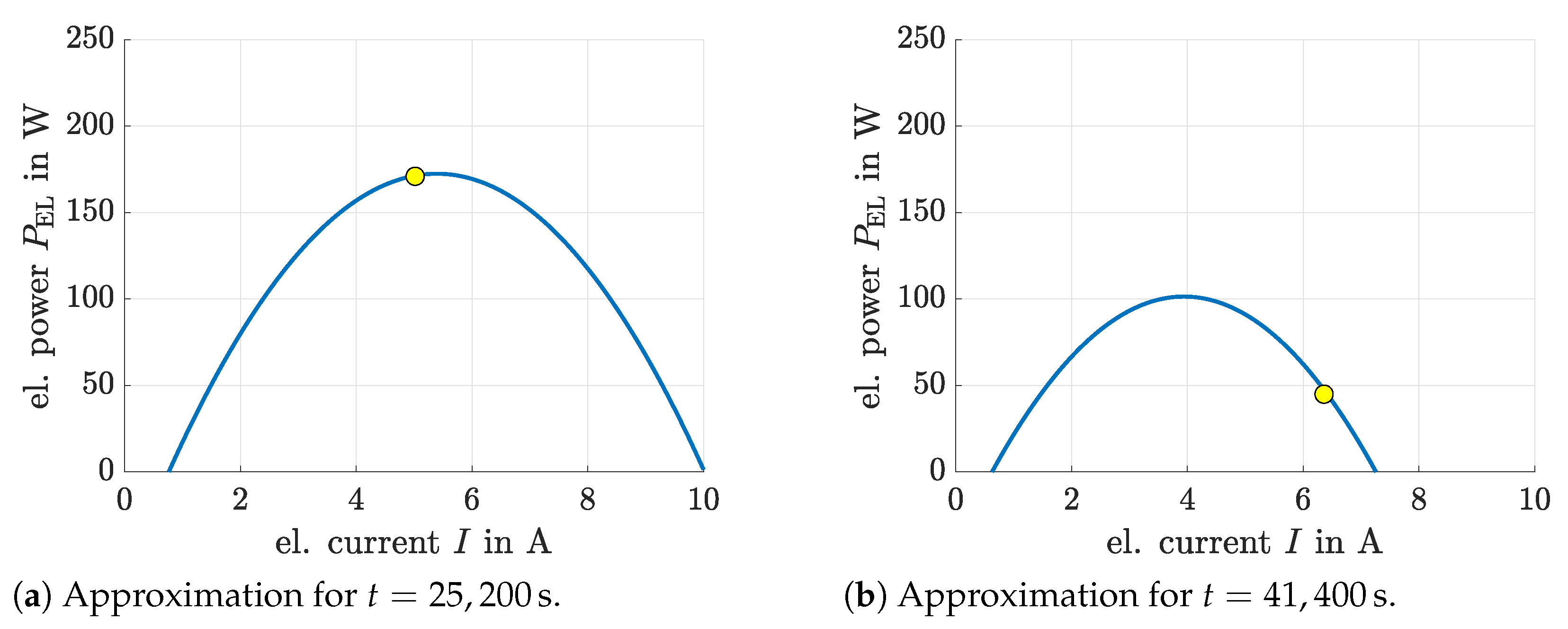
5.1. Identification of Operation in Ohmic Polarization
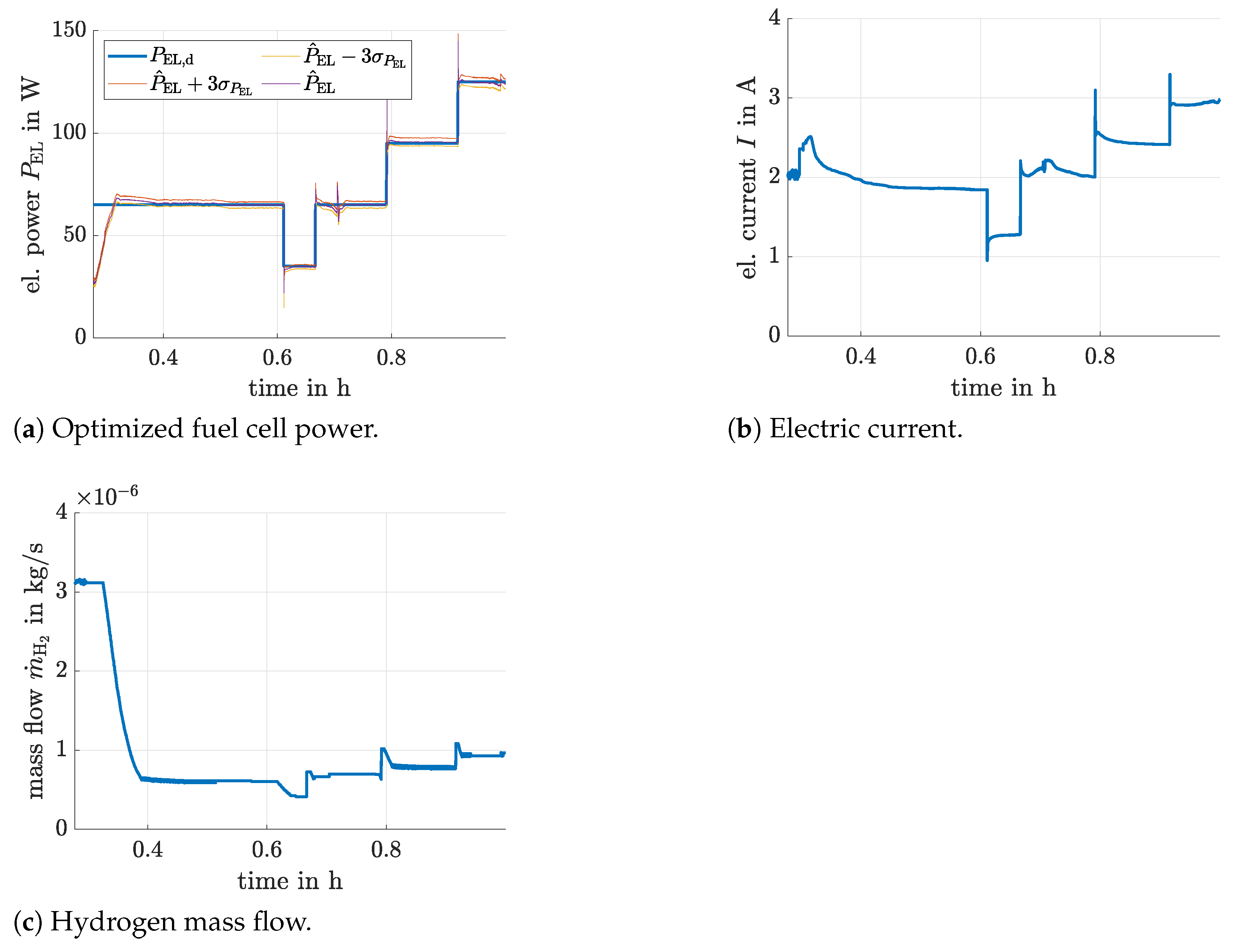
5.2. Validation of the Kalman Filter-Based Input Optimization
- step-wise changes,
- sinusoidal power variations, and
- a smooth transition between operating points that is characterized by the superposition of functions.
6. Conclusions and Outlook on Future Work
Funding
Data Availability Statement
Conflicts of Interest
References
- Pukrushpan, J.; Stefanopoulou, A.; Peng, H. Control of Fuel Cell Power Systems: Principles, Modeling, Analysis and Feedback Design, 2nd ed.; Springer: Berlin, Germany, 2005. [Google Scholar]
- Bove, R.; Ubertini, S. (Eds.) Modeling Solid Oxide Fuel Cells; Springer: Berlin, Germany, 2008. [Google Scholar]
- Stiller, C. Design, Operation and Control Modelling of SOFC/GT Hybrid Systems. Ph.D. Thesis, University of Trondheim, Trondheim, Norway, 2006. [Google Scholar]
- Stiller, C.; Thorud, B.; Bolland, O.; Kandepu, R.; Imsland, L. Control Strategy for a Solid Oxide Fuel Cell and Gas Turbine Hybrid System. J. Power Sources 2006, 158, 303–315. [Google Scholar] [CrossRef]
- Huang, B.; Qi, Y.; Murshed, A. Dynamic Modeling and Predictive Control in Solid Oxide Fuel Cells: First Principle and Data-Based Approaches; John Wiley & Sons: Chichester, UK, 2013. [Google Scholar]
- Huang, B.; Qi, Y.; Murshed, A. Solid Oxide Fuel Cell: Perspective of Dynamic Modeling and Control. J. Process. Control. 2011, 21, 1426–1437. [Google Scholar] [CrossRef]
- Stambouli, A.B.; Traversa, E. Solid Oxide Fuel Cells (SOFCs): A Review of an Environmentally Clean and Efficient Source of Energy. Renew. Sustain. Energy Rev. 2002, 6, 433–455. [Google Scholar] [CrossRef]
- Divisek, J. High Temperature Fuel Cells. In Handbook of Fuel Cells; John Wiley & Sons, Ltd.: Hoboken, NJ, USA, 2010. [Google Scholar]
- Arsalis, A.; Georghiou, G. A Decentralized, Hybrid Photovoltaic-Solid Oxide Fuel Cell System for Application to a Commercial Building. Energies 2018, 11, 3512. [Google Scholar] [CrossRef]
- Weber, C.; Maréchal, F.; Favrat, D.; Kraines, S. Optimization of an SOFC-based Decentralized Polygeneration System for Providing Energy Services in an Office-Building in Tokyo. Appl. Therm. Eng. 2006, 26, 1409–1419. [Google Scholar] [CrossRef]
- Sinyak, Y. Prospects for Hydrogen Use in Decentralized Power and Heat Supply Systems. Stud. Russ. Econ. Dev. 2007, 18, 264–275. [Google Scholar] [CrossRef]
- Dodds, P.E.; Staffell, I.; Hawkes, A.D.; Li, F.; Grünewald, P.; McDowall, W.; Ekins, P. Hydrogen and Fuel Cell Technologies for Heating: A Review. Int. J. Hydrog. Energy 2015, 40, 2065–2083. [Google Scholar] [CrossRef]
- Frenkel, W.; Rauh, A.; Kersten, J.; Aschemann, H. Experiments-Based Comparison of Different Power Controllers for a Solid Oxide Fuel Cell Against Model Imperfections and Delay Phenomena. Algorithms 2020, 13, 76. [Google Scholar] [CrossRef]
- Han, S.; Sun, L.; Shen, J.; Pan, L.; Lee, K.Y. Optimal Load-Tracking Operation of Grid-Connected Solid Oxide Fuel Cells through Set Point Scheduling and Combined L1-MPC Control. Energies 2018, 11, 801. [Google Scholar] [CrossRef]
- Rauh, A.; Dötschel, T.; Aschemann, H. Experimental Parameter Identification for a Control-Oriented Model of the Thermal Behavior of High-Temperature Fuel Cells. In Proceedings of the CD-Proceedings of IEEE International Conference on Methods and Models in Automation and Robotics MMAR, Miedzyzdroje, Poland, 22–25 August 2011. [Google Scholar]
- Rauh, A.; Senkel, L.; Kersten, J.; Aschemann, H. Reliable Control of High-Temperature Fuel Cell Systems using Interval-Based Sliding Mode Techniques. IMA J. Math. Control. Inf. 2016, 33, 457–484. [Google Scholar] [CrossRef]
- Rauh, A.; Senkel, L.; Aschemann, H. Reliable Sliding Mode Approaches for the Temperature Control of Solid Oxide Fuel Cells with Input and Input Rate Constraints. In Proceedings of the 1st IFAC Conference on Modelling, Identification and Control of Nonlinear Systems, MICNON 2015, Saint-Petersburg, Russia, 24–26 June 2015. [Google Scholar]
- Rauh, A.; Senkel, L.; Aschemann, H. Interval-Based Sliding Mode Control Design for Solid Oxide Fuel Cells with State and Actuator Constraints. IEEE Trans. Ind. Electron. 2015, 62, 5208–5217. [Google Scholar] [CrossRef]
- Rauh, A.; Senkel, L.; Auer, E.; Aschemann, H. Interval Methods for the Implementation of Real-Time Capable Robust Controllers for Solid Oxide Fuel Cell Systems. Math. Comput. Sci. 2014, 8, 525–542. [Google Scholar] [CrossRef]
- Rauh, A.; Senkel, L.; Kersten, J.; Aschemann, H. Verified Stability Analysis for Interval-Based Sliding Mode and Predictive Control Procedures with Applications to High-Temperature Fuel Cell Systems. In Proceedings of the 9th IFAC Symposium on Nonlinear Control Systems, Toulouse, France, 4–6 September 2013. [Google Scholar]
- Dötschel, T.; Auer, E.; Rauh, A.; Aschemann, H. Thermal Behavior of High-Temperature Fuel Cells: Reliable Parameter Identification and Interval-Based Sliding Mode Control. Soft Comput. 2013, 17, 1329–1343. [Google Scholar] [CrossRef]
- Abbaker, O.; Wang, H.; Tian, Y. Robust Model-Free Adaptive Interval Type-2 Fuzzy Sliding Mode Control for PEMFC System Using Disturbance Observer. Int. J. Fuzzy Syst. 2020, 22, 2188–2203. [Google Scholar] [CrossRef]
- Aliasghary, M. Control of PEM Fuel Cell Systems Using Interval Type-2 Fuzzy PID Approach. Fuel Cells 2018, 18, 449–456. [Google Scholar] [CrossRef]
- Harrag, A. Modified P&O-Fuzzy Type-2 Variable Step Size MPPT for PEM Fuel Cell Power System; Springer: Singapore, 2021; pp. 363–370. [Google Scholar]
- Rauh, A.; Frenkel, W.; Kersten, J. Kalman Filter-Based Online Identification of the Electric Power Characteristic of Solid Oxide Fuel Cells Aiming at Maximum Power Point Tracking. Algorithms 2020, 13, 58. [Google Scholar] [CrossRef]
- Kalman, R. A New Approach to Linear Filtering and Prediction Problems. Trans. ASME J. Basic Eng. 1960, 82, 35–45. [Google Scholar] [CrossRef]
- Stengel, R. Optimal Control and Estimation; Dover Publications, Inc.: Mineola, TX, USA, 1994. [Google Scholar]
- Anderson, B.; Moore, J. Optimal Filtering; Dover Publications, Inc.: Mineola, TX, USA, 2005. [Google Scholar]
- Razbani, O.; Assadi, M. Artificial Neural Network Model of a Short Stack Solid Oxide Fuel Cell Based on Experimental Data. J. Power Sources 2014, 246, 581–586. [Google Scholar] [CrossRef]
- Xia, Y.; Zou, J.; Yan, W.; Li, H. Adaptive Tracking Constrained Controller Design for Solid Oxide Fuel Cells Based on a Wiener-Type Neural Network. Appl. Sci. 2018, 8, 1758. [Google Scholar] [CrossRef]
- Burstein, G. A Hundred Years of Tafel’s Equation: 1905–2005. Corros. Sci. 2005, 47, 2858–2870. [Google Scholar] [CrossRef]
- Tafel, J. Über die Polarisation bei kathodischer Wasserstoffentwicklung. Z. Phys. Chem. StÖchiometrie Verwandtschaftslehre 1905, 50, 641–712. (In German) [Google Scholar] [CrossRef]
- Rauh, A.; Kersten, J.; Frenkel, W.; Kruse, N.; Schmidt, T. Physically Motivated Structuring and Optimization of Neural Networks for Multi-Physics Modeling of Solid Oxide Fuel Cells. Math. Comput. Model. Dyn. Syst. 2021. under review. [Google Scholar]
- Kanjilal, P.; Dey, P.; Banerjee, D. Reduced-Size Neural Networks Through Singular Value Decomposition and Subset Selection. Electron. Lett. 1993, 29, 1516–1518. [Google Scholar] [CrossRef]
- Garrappa, R. Predictor-Corrector PECE Method for Fractional Differential Equations. MATLAB Central File Exchange. Available online: www.mathworks.com/matlabcentral/fileexchange/32918-predictor-corrector-pece-method-for-fractional-differential-equations (accessed on 14 January 2020).
- Tee, K.; Ge, S.S.; Tay, E.H. Barrier Lyapunov Functions for the Control of Output-Constrained Nonlinear Systems. Automatica 2009, 45, 918–927. [Google Scholar] [CrossRef]
- Rauh, A.; Senkel, L. Interval Methods for Robust Sliding Mode Control Synthesis of High-Temperature Fuel Cells with State and Input Constraints. In Variable-Structure Approaches: Analysis, Simulation, Robust Control and Estimation of Uncertain Dynamic Processes; Rauh, A., Senkel, L., Eds.; Math. Eng.; Springer: Berlin, Germany, 2016; pp. 53–85. [Google Scholar]
- Cont, N.; Frenkel, W.; Kersten, J.; Rauh, A.; Aschemann, H. Interval-Based Modeling of High-Temperature Fuel Cells for a Real-Time Control Implementation Under State Constraints. In Proceedings of the 21st IFAC World Congress, Berlin, Germany, 12–17 July 2020. [Google Scholar]
- Nocedal, J.; Wright, S.J. Numerical Optimization, 2nd ed.; Springer: New York, NY, USA, 2006. [Google Scholar]
- Rutishauser, H. Theory of Gradient Methods. In Refined Iterative Methods for Computation of the Solution and the Eigenvalues of Self-Adjoint Boundary Value Problems; Birkhäuser Basel: Basel, Switzerland, 1959; pp. 24–49. [Google Scholar]
- Rauh, A.; Kersten, J. Verification and Reachability Analysis of Fractional-Order Differential Equations Using Interval Analysis. In Electronic Proceedings in Theoretical Computer Science, Proceedings 6th International Workshop on Symbolic-Numeric methods for Reasoning about CPS and IoT, online, 31 August 2020; Dang, T., Ratschan, S., Eds.; Open Publishing Association: Den Haag, The Netherlands, 2021; Volume 331, pp. 18–32. [Google Scholar] [CrossRef]
- Rauh, A.; Kersten, J.; Aschemann, H. Interval-Based Verification Techniques for the Analysis of Uncertain Fractional-Order System Models. In Proceedings of the 18th European Control Conference ECC2020, Saint Petersburg, Russia, 12–15 May 2020. [Google Scholar]


| Variable | Physical Meaning |
|---|---|
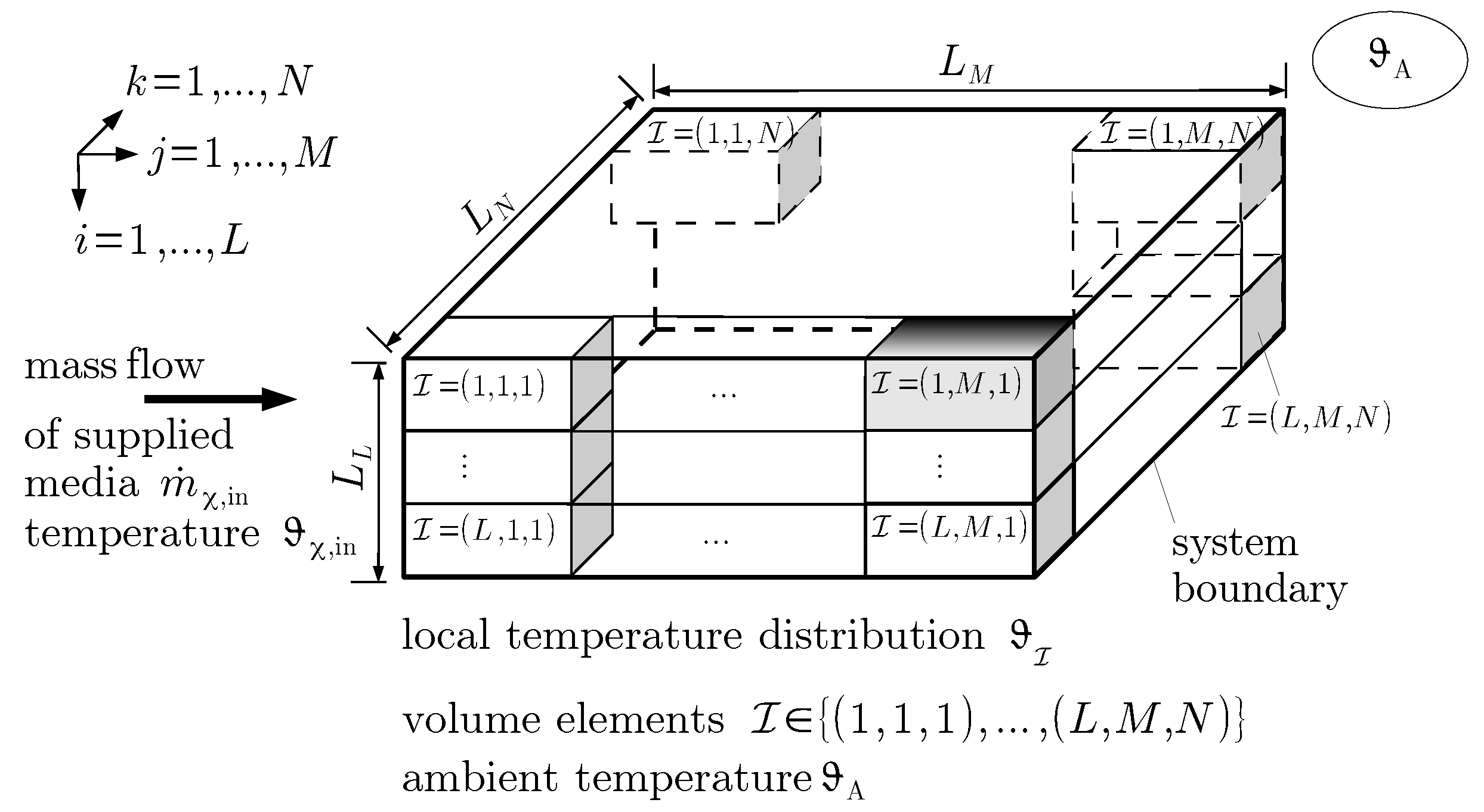
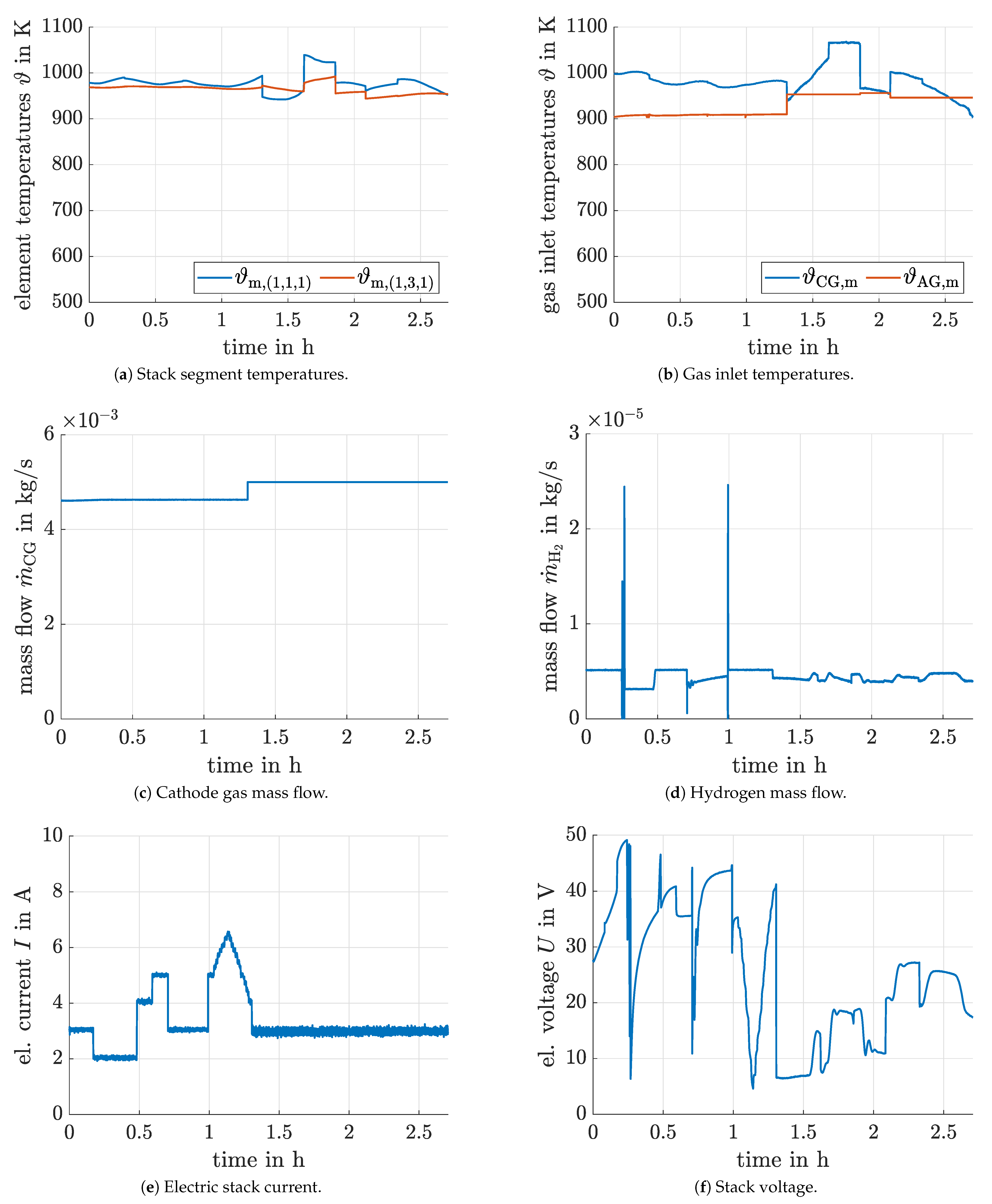
| , , | stack segment temperatures, discretization in the direction of gas mass flow |
| I | electric stack current |
| U | electric stack voltage |
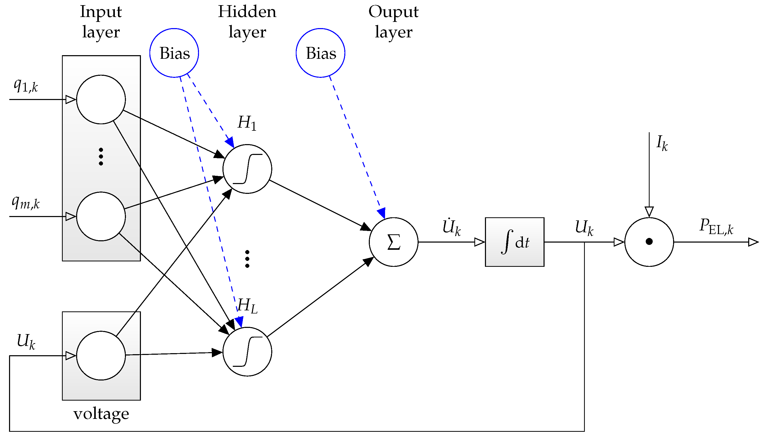
| temporal derivative of the electric stack voltage | |
| electric power | |
| mass flow of supplied cathode gas (preheated air) | |
| gas inlet temperature at the cathode | |
| nitrogen mass flow (anode) | |
| hydrogen mass flow (anode) | |
| gas inlet temperature at the anode | |
| ambient temperature | |
| subscript index | measured variable (added for distinction from simulation and estimation results) |
| subscript index k | discrete time index (sampling time: ) |
| Network Type | Network Inputs | ||||||||||
|---|---|---|---|---|---|---|---|---|---|---|---|
| I | U | ||||||||||
| static voltage prediction (Figure 2, Figure 7 and Figure 9) | ✔ | ✘ | ✔ | ✔ | ✘ | ✘ | ✔ | ✔ | ✔ | ✔ | ✘ |
| dynamic voltage prediction (Figure 5) | ✔ | ✘ | ✔ | ✔ | ✔ | ✘ | ✔ | ✔ | ✔ | ✔ | ✘ |
| Order n | Order | |||||||
|---|---|---|---|---|---|---|---|---|
| 1 | − | − | − | − | ||||
| 3 |
| No. | Network Type | Optimized? | Training Data | Hidden Neurons | RMS | ||||
|---|---|---|---|---|---|---|---|---|---|
| U | |||||||||
| Figure 2 | voltage prediction (static) | ✘ | ✘ | ✘ | ✘ | ✘ | ✔ | 30 | |
| Figure 2 | voltage prediction (static) | ✔ | ✘ | ✘ | ✘ | ✘ | ✔ | 7 | |
| Figure 5 | voltage prediction (dynamic) | ✘ | ✘ | ✘ | ✘ | ✔ | ✘ | 30 | |
| Figure 5 | voltage prediction (dynamic) | ✔ | ✘ | ✘ | ✘ | ✔ | ✘ | 9 | |
| Figure 7 | voltage prediction () | ✘ | ✘ | ✘ | ✘ | ✘ | ✔ | 30 | |
| Figure 7 | voltage prediction () | ✔ | ✘ | ✘ | ✘ | ✘ | ✔ | 7 | |
| Figure 9 | voltage prediction (, ) | ✘ | ✘ | ✘ | ✘ | ✘ | ✔ | 30 | |
| Figure 9 | voltage prediction (, ) | ✔ | ✘ | ✘ | ✘ | ✘ | ✔ | 7 | |
| Figure 9 | voltage prediction (, ) | ✘ | ✘ | ✘ | ✘ | ✘ | ✔ | 30 | |
| Figure 9 | voltage prediction (, ) | ✔ | ✘ | ✘ | ✘ | ✘ | ✔ | 7 | |
| System Model | Reference Signal | RMS |
|---|---|---|
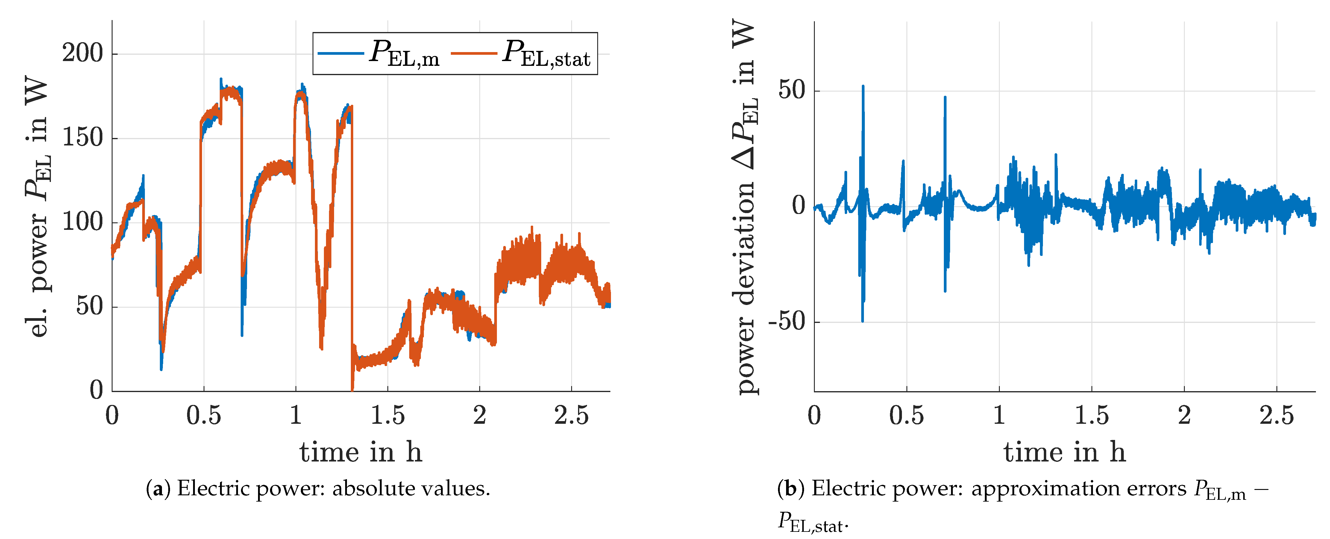
| Figure 2 | step-wise changes | |
| Figure 2 | sinusoidal | |
| Figure 2 | smooth | |
| Figure 7 | step-wise changes | |
| Figure 7 | sinusoidal | |
| Figure 7 | smooth | |
| Figure 9 () | step-wise changes | |
| Figure 9 () | sinusoidal | |
| Figure 9 () | smooth |
Publisher’s Note: MDPI stays neutral with regard to jurisdictional claims in published maps and institutional affiliations. |
© 2021 by the author. Licensee MDPI, Basel, Switzerland. This article is an open access article distributed under the terms and conditions of the Creative Commons Attribution (CC BY) license (http://creativecommons.org/licenses/by/4.0/).
Share and Cite
Rauh, A. Kalman Filter-Based Real-Time Implementable Optimization of the Fuel Efficiency of Solid Oxide Fuel Cells. Clean Technol. 2021, 3, 206-226. https://doi.org/10.3390/cleantechnol3010012
Rauh A. Kalman Filter-Based Real-Time Implementable Optimization of the Fuel Efficiency of Solid Oxide Fuel Cells. Clean Technologies. 2021; 3(1):206-226. https://doi.org/10.3390/cleantechnol3010012
Chicago/Turabian StyleRauh, Andreas. 2021. "Kalman Filter-Based Real-Time Implementable Optimization of the Fuel Efficiency of Solid Oxide Fuel Cells" Clean Technologies 3, no. 1: 206-226. https://doi.org/10.3390/cleantechnol3010012
APA StyleRauh, A. (2021). Kalman Filter-Based Real-Time Implementable Optimization of the Fuel Efficiency of Solid Oxide Fuel Cells. Clean Technologies, 3(1), 206-226. https://doi.org/10.3390/cleantechnol3010012