Abstract
Efforts have been underway worldwide to reintroduce seawater to many historically diked salt marshes for restoration of tidal flow and associated estuarine habitat. Seawater restoration to a diked Cape Cod marsh was simulated using the computer program PHREEQC based on previously conducted microcosm experiments to better understand the associated timing and sequence of multiple biogeochemical reactions and their implications to aquatic health. Model simulations show that acidic, reducing waters with high concentrations of sorbed ferrous iron (Fe[II]), aluminum (Al), sulfide (S2−), ammonia (NH4+ + NH3), and phosphate (PO43−) are released through desorption and sediment weathering following salination that can disrupt aquatic habitat. Models were developed for one-dimensional reactive transport of solutes in diked, flooded (DF) marsh sediments and subaerially exposed, diked, drained (DD) sediments by curve matching porewater solute concentrations and adjusting the sedimentary organic matter (SOM) degradation rates based on the timing and magnitude of Fe(II) and S2− concentrations. Simulated salination of the DD sediments, in particular, showed a large release of Al, Fe(II), NH4+, and PO43−; the redox shift to reductive dissolution provided higher rates of SOM oxidation. The sediment type, iron source, and seasonal timing associated with seawater restoration can affect the chemical speciation and toxicity of constituents to aquatic habitat. The constituents of concern and their associated complex biogeochemical reactions simulated in this study are directly relevant to the increasingly common coastal marsh salination, either through tidal restoration or rising sea level.
1. Introduction
Historical blockage of tidal exchange within salt marshes through diking reduces or eliminates seawater interaction and has resulted in the freshening of surface water and marsh porewater. This diking of coastal wetlands has resulted in water-quality problems such as hypoxia and acidified leachate [1,2,3], the loss of shellfish and fisheries habitat and biodiversity [4,5,6,7], loss of buffer from sea-level rise [8], and stagnated freshwater ponds that host mosquitos and midges [1]. Diking of coastal wetlands has been practiced extensively for hundreds of years (yrs) in western Europe and the North Atlantic [5]. In southern New England, pre-colonial salt marshes have been ditched, drained, and diked for livestock grazing, hay production, and later insect control to the point where about 50 to 70 percent were destroyed [9,10]. In the contiguous U.S., it has been estimated that 5000–6000 km2 of wetland or potential wetland space in the intertidal zone has impaired tidal exchange, behind dikes, levees, or transportation infrastructure [11,12,13]. These concerns with diking have led to widespread efforts in salt marsh restoration, including the removal of tidal restrictions. Restoration of disconnected saline tidal flows is intended to reverse the water-quality problems listed above and has also been found to substantially reduce emission of CO2 and CH4 [11,12,13,14]. However, restoration of diked coastal marshes from fresh to saltwater can cause substantial eutrophication from the release of freshwater sediment-derived nutrients and also the release of acidity and iron (Fe) from Fe sulfide minerals [4,15]. Furthermore, the effects of sea-level rise and subsequent increased freshwater salinity on aquatic habitat are complex and not well understood [16,17]. Therefore, understanding these diked marsh systems can help inform coordination of restoration efforts to avoid potential problems.
The response of marsh biogeochemistry to tidal restoration depends on the flood-tide depth and duration and their effects on sediment, porewater, and substrate composition [4]. Diked marshes are generally either seasonally flooded or perennially drained depending on the freshwater drainage capacity of culverts and creek systems [5]. Diked marshes with sediments that are seasonally flooded (referred to as “diked, seasonally flooded” or DF) accumulate peat of higher organic content than salt marsh peat [4,18,19] because the inorganic sediment supply normally imported by flood tides is limited [20] and the decomposition in freshwater peats, dominated by methanogens, is slow [21]. Furthermore, porewater nutrient concentrations are low [5], probably as a result of both anoxic conditions, which are conducive to denitrification, and sorption of ammonium (NH4+) and phosphate (PO43−) to surfaces. Seawater restoration in these diked wetlands should cause nutrient release because the increase in SO42− concentrations and corresponding SO42− reducing conditions will enhance SOM degradation, which increases pH and production of bicarbonate, and subsequently leads to desorption of NH3 [4]. Diked marshes with sediments that were drained (referred to as “diked, drained” or DD) resulted in air penetration into previously anoxic sediments, subsequent oxidation of SOM and Fe sulfide minerals, and release of acidity, dissolved Fe, Al, and nutrients including NH4+ and PO43−. DF and DD sediments represent the end members in these diked marsh systems, and understanding the way they respond to seawater restoration is critical in assessing the resulting biogeochemical changes.
Acidic soils are common in estuaries, and their inundation by tidal restoration or sea-level rise can lead to significant amounts of desorption and ion exchange [4,16,22,23]. The major distinction between sorption (adsorption and absorption) and exchange is that geochemical model equations for sorption use the concentration of one chemical only, and ignore the effects of other solutes, whereas exchange involves the replacement of one chemical for another at the solid surface [24,25]. The behavior of PO43− in aqueous systems, for example, can be affected by both ion exchange and sorption processes [26,27]. Geochemical models such as PHREEQC can simulate both sorption/desorption and exchange; sorption/desorption can be modeled as surface complexation reactions (such as the Dzombak and Morel [28] model) and exchange can be modeled using several conventions such as Gaines–Thomas [29]. Sorption (or desorption) is generally used herein to describe both sorption/desorption and ion-exchange reactions.
The Herring River estuary in Wellfleet, Massachusetts (MA) (Figure 1) is an example of such a diked marsh system, and the third and largest salt marsh restoration project (445 hectares) is currently underway. The ocean tides were blocked from the Herring River following construction of the Chequesset Neck Road Dike in 1909, causing a transition from salt marsh to freshwater wetlands. Considerable concern over the marsh restoration of the Herring River exists because (1) a stressed river herring population that includes alewife (Alosa pseudoharengus) and blueback herring (Alosa aestivalis) [30] migrates through the river into upstream kettle ponds; (2) acidic waters with low dissolved oxygen (DO) and high Fe and nutrient concentrations, common to diked marsh creeks, are released during seawater interaction and intense rain events [3,31]; and (3) these waters are received by Wellfleet Harbor, which contains productive shellfish aquaculture that is sensitive to water-quality degradation. Out of concern that this marsh restoration program could severely affect the Wellfleet Harbor Area of Critical Environmental Concern [32], sediment cores were collected from areas near and in the area of anticipated restoration and used in marsh sediment microcosm salination experiments to assess the biogeochemical effects of seawater intrusion, as described in Portnoy and Giblin [4,5]. Sediment microcosm experiments are helpful in understanding marsh restoration effects on porewater biogeochemistry [4,5] but are constrained by the given length of the experiments, rates of porewater flow, and variations in the sediment biogeochemistry. Geochemical modeling is necessary for improved understanding of coastal marsh biogeochemistry by allowing the calculation of multiple complex biogeochemical reactions coupled with varying response factors such as mineralogy, sediment properties, and flow rates.
In this study, biogeochemical modeling was used to describe seawater reintroduction to diked marsh sediments based on microcosm experiments using sediment cores from Herring River marsh and the North Sunken Meadow salt marsh in Eastham, MA (Figure 1 and Figure 2) [4,5]. The reactive-transport model simulations help relate the complex biogeochemical changes observed in the microcosms after salination [4] to chemical reactions and reaction rates so that the timing and sequence of these reactions (including desorption and a redox shift to SO42− reduction) can be simulated over longer time periods for the resalination of the Herring River, and potentially other diked marsh settings.
The USGS computer program PHREEQC (“pH-redox-equilibrium model in the C programming language”; [29]) was used to simulate one-dimensional reactive transport in diked salt marsh sediments. The models account for spatial and temporal changes in seawater flowing through freshwater sediments, transport of associated chemical constituents, and a set of chemical reactions including desorption of constituents, SOM decomposition, and dissolution and precipitation of iron-bearing minerals. The Supplementary Materials (SM) provides further details on (SM File S1) the PHREEQC [29] model input and selected output files, along with aquatic life water-quality criteria for simulated pH and solute concentrations, and (SM File S2) the calibration of microcosm models. The PHREEQC model input and selected output files, and instructions on running the model, are also available as a USGS data release [33].

Figure 1.
Location of the Herring River study area, Wellfleet, Massachusetts, and location of the North Sunken Meadow core sample collection site. Modified from [34].
Figure 1.
Location of the Herring River study area, Wellfleet, Massachusetts, and location of the North Sunken Meadow core sample collection site. Modified from [34].


Figure 2.
Herring River watershed basin boundary with the major soil series as determined by the Natural Resources Conservation Service [35]. The Freetown and Swansea soil series (green) are primarily diked, flooded (DF) soils that occur primarily on upgradient arms of the marsh system, where groundwater levels are presumably higher in elevation. The Maybid soil series (brown) are primarily diked, drained sediments with acidic pH. Modified from [36]).

2. Methods
Geochemical models were first developed and calibrated with PHREEQC [29] using data from the Herring River microcosm experiments [4] (Appendix A, Supplementary Materials Files S1 and S2); then “basecase” models were used to simulate a single flow velocity over longer time periods (Table 1) and with varying Fe(III) source minerals. Biogeochemical reactions associated with marsh restoration that need to be simulated are discussed in Section 2.1, and development and calibration of the PHREEQC models are detailed in Section 2.2. Development of basecase models that are used to vary biogeochemical conditions and simulation times are discussed in Section 2.3.

Table 1.
Column conditions and saltwater flow rates used in the PHREEQC simulations for cores representing diked, flooded (DF) sediments, and diked, drained (DD) sediments for the Herring River, Massachusetts [33]. %, percent; h, hour; mo, month; yr, year.
Table 1.
Column conditions and saltwater flow rates used in the PHREEQC simulations for cores representing diked, flooded (DF) sediments, and diked, drained (DD) sediments for the Herring River, Massachusetts [33]. %, percent; h, hour; mo, month; yr, year.
| Simulation | Microcosm Flow, Saltwater (Solution 0) | Porosity (%) | Number of Pore Volumes | Number of Shifts | Time per Shift (Seconds) | Velocity a (Meters/Second) | |
|---|---|---|---|---|---|---|---|
| Volume (Liters) | Time Period | DF/DD | |||||
| Microcosm column experiment models [4] | 10 | 12 h | 90/55 | 1.38/2.29 | 62/103 | 687/419 | 1.4 × 10⁻⁵/2.4 × 10−5 |
| 3 | 3 mos | 90/55 | 0.42/0.69 | 18.9/30.9 | 412,031/251,793 | 2.4 × 10⁻⁸/3.97 × 10−8 | |
| 1.5 | 10 mos | 90/55 | 0.21/0.34 | 9.44/15.4 | 2,746,872/1,678,618 | 3.7 × 10⁻⁹/5.96 × 10−9 | |
| 3.5 | 7 mos | 90/55 | 0.49/0.80 | 22/36 | 824,062/503,585 | 1.2 × 10⁻⁸/1.99 × 10−8 | |
| Basecase models | 72.9 | 12 yrs | 90/55 | 10.2/16.7 | 458/750 | 828,818/506,573 | 1.2 × 10⁻⁸/1.97 × 10−8 |
| 605 | 100 yrs | 90/55 | 9.9 × 10⁴/1.6 × 105 | 3808/ 6230 | 828,718/ 506,543 | 1.2 × 10⁻⁸/1.97 × 10−8 | |
a The velocity of water in each cell is determined by the length of the cell (0.01 m) divided by the time per shift.
2.1. Study Area and Marsh Restoration Biogeochemistry
Partial restriction on inflowing tides at Herring River (Figure 1) has resulted in lower mean sea level landward of the dike so that surficial sediments in wetland areas adjacent to the Herring River main stem have been dewatered (Figure 2). In 2017–2018, the typical tide range on the upstream side of the Herring River tide-control structure was about 0.67 m, whereas on the downstream side (Wellfleet Harbor), it was about 3.1 m [34]. Restoration of the Herring River marsh involved demolition of the existing dike and removal of tidal restrictions in a phased approach by outfitting the new bridge with sluice gates that will allow water and salinity levels to rise gradually over the coming decade, enabling the ecosystem to grow back more naturally. As of March 2025, tidal flow has begun to be transitioned from the old dike culverts to the tidal gates of the new Chequessett Neck Road Bridge and Water Control Structure, but the restricted tidal flow remains the same and the restoration process will not begin until construction is complete in another year [37].
Reflooding with seawater during the Herring River restoration would likely result in rapid infiltration into unsaturated DD sediments, as seawater infiltrates pore spaces and replaces soil gas, but relatively slowly in the DF sediment, where freshwater will eventually be replaced by saltwater.
Based on studies of salt marsh restorations and microcosm experiments [4,5], immediate re-entry of seawater into diked and seasonally flooded and drained marshes results in significant die off of freshwater biomass and subsequent oxidation of SOM coupled to the reduction of oxygen (Equation (1)), ferric oxyhydroxides (Equation (2)), and SO42− (Equation (3)) and results in anoxic conditions and increased concentrations of alkalinity, Fe(II), and S2− in sediments.
CH2O(s) + O2(g) → CO2(aq) + H2O(l)
CH2O(s) + 4Fe(OH)3(s) + 7H+(aq) → 4Fe2+(aq) + HCO3−(aq) + 10H2O(l)
CH3COOH(s) + SO42−(aq) + 2H+(aq) → H2S(aq) + 2CO2(aq) + 2H2O(l).
Ferric hydroxides can also be reduced by dissolved S2− [38]. These biogeochemical reactions in saltmarsh sediments are analogous to those described for marine sediments during diagenesis [39] and follow the well-known sequence of microbially mediated reactions that proceed from most energetically favorable to less favorable reactions. SOM is first oxidized by oxygen, then by nitrate, Fe(III), SO42−, and finally carbon (C) through methanogenesis by the hydrogenotrophic pathway (Equation (4)):
or by the acetoclastic pathway [40]. Fe(II) or Fe(III) can react with the S2− to form Fe monosulfides (FeS), such as mackinawite (Equation (5)):
and eventually Fe disulfide (FeS2) such as pyrite, which can take place rapidly with H2S as a reactant [41,42,43]. Large amounts of NH4+ and PO43− could be released by desorption and cation exchange as pH rises, and from reductive dissolution of Fe(III) hydroxide minerals, causing eutrophication; P is also released from sorption sites.
HCO3−(aq) + H+(aq) + 4H2 → CH4(aq) + 3H2O(l)
2FeOOH(s) + 3HS−(aq) → 2FeSmack + S0(aq) + 3OH−(aq) + H2O(l)
The aeration of peat marsh sediments can cause oxidation of pyrite (Equation (6)):
that generates highly acidic (pH < 4) porewaters rich in dissolved Fe(II) and SO42− and can lead to fish mortality [1,2,44]. The Fe(II) initially released may be oxidized to Fe(III), which is a more effective oxidant than oxygen [45,46,47], and can be solubilized by organic ligands [48]. The Fe2+ oxidizes and may precipitate Fe(III) hydroxide and Fe(III) hydroxysulfate minerals, such as goethite (Equation (7)) or jarosite minerals (Equations (8) and (9)):
FeS2(s) + 7/2O2(g) + H2O(l) → Fe2+(aq) + 2SO42−(aq) + 2H+(aq)
Fe(OH)2+(aq) + H2O(l) ↔ FeOOH(goethite) + 4H+(aq)
3Fe3+(aq) + M+(aq) + 2HSO4−(aq) + 6H2O(l) → MFe3(SO4)2(OH)6(jarosite) + 8H+(aq)
3Fe3+(aq) + NH4+(aq) + 2HSO4−(aq) + 6H2O(l) → NH4Fe3(SO4)2(OH)6(jarosite-amm) + 8H+(aq).
Jarosite is commonly found in acid-SO42− soils as a byproduct of pyrite oxidation in DD sediments [5] and is well-documented to form at low pH [49]; M+ can include monovalent cations such as Na+ or NH4+, as in ammonium jarosite or “jarosite-amm” (Equation (9)). Goethite is the predominant secondary phase on pyrite surfaces under alkaline conditions [50]. Cations such as Na+ can compete with Fe2+ for sorption or exchange sites (X) on goethite and other Fe oxide minerals [51] such as Na+ for FeX2 (Equation (10)):
and can result in increased dissolved Fe2+ concentrations [52,53]. The biogeochemical cycling of Fe in estuaries has a strong seasonal component because of the integral role of organic ligands that are generated and decomposed during the growing season [48].
FeX2(exch) + 2Na+(aq) ↔ 2NaX(exch) + Fe2+(aq)
Fe sulfide mineral (FeS or FeS2) oxidation (Equation (6)), Fe(II) oxidation, and jarosite precipitation (Equations (7)–(9)) generate acidity that can be harmful to aquatic life. The United States Environmental Protection Agency (USEPA) water-quality criteria for pH in freshwater suggest a range of 6.5 to 9; pH below this range physiologically stresses many species and can result in decreased reproduction, decreased growth, disease, or death [4,54]. NH3 is toxic to saltwater aquatic life, with chronic and acute values of 0.23 mg/L (0.016 mmol/L) and 1.7 mg/L (0.12 mmol/L), respectively [55]. NH4+ is the dominant species at pH < 9.2 and is likely mobilized by desorption during salination [4,56]. Al is also mobilized during salination of diked marshes and is a particular concern for aquatic life, particularly fish [57].
2.2. Microcosm Geochemical Models and Calibration
Previous microcosm experiment data [4] were evaluated and used to develop and calibrate one-dimensional models using PHREEQC [29] to simulate the resalination of DF and DD sediments at the Herring River after dike removal. Two microcosm experiment models were created, one for salination of each sediment type (DF and DD) used in the experiments. Model assumptions and set up for the sediment cores are described in Section 2.2.1. Model calibration involved iteratively curve fitting simulated with measured solute concentrations to establish SOM degradation rates (Section 2.2.2) and calculating the number of exchange sites and the log k for H+ to obtain the simulated pH best fit with the Portnoy and Giblin [4] data.
2.2.1. Model Assumptions and Set Up
The PHREEQC models assume that fresh porewater initially fills the sediment cores (Figure 3) and is replaced by an influx of seawater for 20 months, to be consistent with Portnoy and Giblin [4] experiments. In simulations of DF and DD sediments, seawater passed through the columns after about 8 h and 5 h, respectively. The models had similar initial solute concentrations of freshwater, but the pH, Fe(II), and ammonium concentrations differed. Seawater concentrations (Table 1) were the same for both microcosm models.
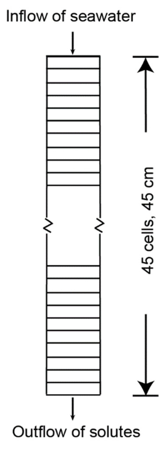
Figure 3.
Diagram of biogeochemical model for which geochemical reactions and solute movement through microcosm cores [4,5] were simulated.
PHREEQC is one of the most commonly used codes for a variety of water chemistry studies, including the combined effects of complex biogeochemical reactions and transport [17,58,59]. PHREEQC is ideal for biogeochemical simulations such as tidal marsh restoration because it implements several types of aqueous models that have capabilities for calculations including speciation and saturation index, and 1-D transport with reactions including aqueous, mineral, gas, solid–solution, surface-complexation (used to model sorption and desorption) and ion-exchange equilibria, and kinetic reaction [29]. It also has a built-in BASIC interpreter that allows for complex reaction rate laws and output post-processing options [29]. PHREEQC was used with the phreeqc.dat thermodynamic database; input files, concentration-time plots, and selected output are provided in Supplementary Material (SM) File S1 (Tables S1–S10) and in Brown [33]. Details on model calibration are provided in SM File S2.
The PHREEQC option for advective-reactive transport simulation with reversible and irreversible chemical reactions [29] was used for these models. This study utilizes site-specific data and processes that are common to other tide-restricted marsh systems worldwide that contain harmful or toxic levels of acidity and constituents including S2−, NH4+, Al, and Fe(II). Although the 1-D flow assumptions are reasonable for simulations of column experiments, actual field conditions include 3-D flow that is tide dependent, heterogeneous hydraulic properties, and sediment biogeochemistry that varies laterally beyond the extent of the cores. These conditions will result in uncertainty that is not accounted for in this study, but the models allow a simplified understanding of the biogeochemical reactions and solute transport rates. Mineral phases and SOM are assumed to react to equilibrium with the aqueous phase throughout the simulations (Table 2). Simulated flow of porewater and seawater through the sediments did not include the processes of diffusion or dispersion.
Table 2.
Rates of sedimentary organic matter (SOM) degradation and mineral dissolution and precipitation reactions used in the resalination models of diked, flooded (DF) sediments and diked, drained (DD) sediments. Note that oxygen reduction and denitrification are not significant to oxidation of carbon; PHREEQC simulations show that dissolved oxygen and any existing nitrate are reduced very quickly after sediments are filled with seawater. Model calibration is described in SM File S2.
| Reaction Number | Reaction | Reaction Type | Equation | Rates (1/s): Determined by Calibration for DF Sediments | Rates (1/s): Determined by Calibration for DD Sediments |
|---|---|---|---|---|---|
| 1 | Oxidation of SOM by reduction of Fe(III) [ammonium jarosite is source of the Fe(III) used in the model] | Redox, kinetically controlled | DOM a + 4x Fe3+4xOH− → xCO2(g) + 4x Fe2+ + 3/xH2O + y NH3 + z H3PO4 | Rate = 3.5 × 10⁻⁹ | Rate = 7 × 10⁻⁹ |
| 2 | Oxidation of SOM by reduction of SO42− | Redox, kinetically controlled | DOM a + (x/2)SO42− + (y-2z)CO2 + (y-2z)H2O → (x/2)H2S + (x+y−2z)HCO3− + yNH4+ + zHPO42− | IF(tot(“Fe(+3)”) ≤ 2 × 10⁻⁶, THEN rate = 2.5 × 10⁻¹⁰ | IF(tot(“Fe(+3)”) ≤ 2 × 10⁻⁶, THEN rate = 1.76 × 10⁻⁹ |
| 3 | Oxidation of SOM by methanogenesis | Redox, kinetically controlled | DOM a + (y−2z)H2O → x/2CH4 + (x−2y+4z/2)CO2 + (y−2z)HCO3− + yNH4+ + zHPO42− | IF (tot(“Fe(+3)”) ≤ 2 × 10⁻⁶, AND (tot(“SO42−)”) ≤ 2 × 10⁻⁶, THEN rate = 3 × 10⁻¹¹ | IF (tot(“Fe(+3)”) ≤ 2 × 10⁻⁶, AND (tot(“SO42−)”) ≤ 2 × 10⁻⁶, THEN rate = 1.76 × 10⁻¹⁰ |
| 4 | FeS precipitation | Equilibrium | FeS = Fe+2 + S−2 | NA | NA |
| 5 | Al(OH)3 (amorphous) precipitation and dissolution | Equilibrium | Al(OH)3 + 3H+ = Al+3 + 3 H2O | NA | NA |
a DOM = (CH2O)x(NH3)y(H3PO4)z, where x, y, z represent the C:N:P ratios, respectively [60].
The microcosm core dimensions for both models were incorporated into a model grid that uses 45 1 cm cells for the 45 cm core length (Figure 3), with a core volume of 7.95 L. For the two PHREEQC models (Tables S1a,b and S2a,b), the sediments in the columns were initially assumed to be filled with fresh porewater as defined in solutions 1–45 and equilibrated with the DF and DD sediments, respectively (Table 3). Establishing the initial chemistry involved assigning surface exchange sites, solid phase reactant concentrations, kinetics, and solution concentrations for each cell (Table 3 and Table 4). The infilling seawater solution (“Solution 0”) was then introduced to the column, and transport was modeled by “shifting” solution 0 to cell 1, the solution in cell 1 to cell 2, and so on until solution 45 is shifted to cell 45, which is equilibrated with exchange 45, surface 45, equilibrium phases 45, and kinetics 45. The keywords, including “exchange”, “surface”, “equilibrium phases”, and “kinetics”, define the input for PHREEQC, as explained in Parkhurst and Appelo [29]. “Exchange” defines the exchange assemblage composition, “surface” defines the composition of surfaces, “equilibrium phases” defines a singular phase that reacts reversibly, and “kinetics” specifies kinetic reactions and parameters for reactive-transport calculations. The number of cell shifts and the time per shift used in the simulation are shown in Table 1. At every time step, the speciation of the solution and its reaction with sediments was computed.
Table 3.
Solution chemistry of diked, flooded (DF) and diked, drained (DD) sediments and artificial seawater used in PHREEQC simulations of Portnoy and Giblin [4] microcosm experiments. Freshwater chemistry is from [4] except as noted, using freshwater and column-bound concentrations from the same types of cores and at the same depth. Concentrations in mmol/L.
| Constituent or Property | DF Solution 1–45 | DD Solution 1–45 | Seawater Composition, Solution 0 |
|---|---|---|---|
| Temperature °C | 25 | 25 | 25 |
| pH | 6.7 | 4 | 8.5 a |
| pe | -- | -- | 8.45 |
| Na | 0.026 a | 0.026 a | 468 c |
| Ca | 0.004 a | 0.004 a | 10.2 c |
| Mg | 0.0015 a | 0.0015 a | 53.2 c |
| K | 0.001 a | -- | 10.2 c |
| Cl | 0.040 | 0.715 a | 545 c |
| S(6), sulfate | -- | -- | 28.2 c |
| Alkalinity as HCO3- | 4 a | 0.1 a | 2.3 c |
| N(-3), ammonium | 0.001 | 0.075 a | - |
| S2− | 0.1 a | 0 a | -- |
| P | 0.001 b | 0.002 a | -- |
| Fe(II) | 0.0001 a | 0.1 a | -- |
| Fe(III) | 0.0001 a | 0.001 | -- |
| Si | -- | -- | 0.07 c |
| O(0), diss. oxygen | 0.01 | 0.01 | 0.75 |
| Al | 0.01 a | 0.3 a | -- |
a Generally based on Portnoy and Giblin [4], Portnoy and Giblin [5]; b fit parameter—for phosphorus DF and aluminum DF; c Nordstrom, et al. [61].
Table 4.
Ion-exchange and surface complexation sites for diked, flooded (DF) and diked, drained (DD) sediments used in PHREEQC simulations of Portnoy and Giblin [4] microcosm experiments.
Table 4.
Ion-exchange and surface complexation sites for diked, flooded (DF) and diked, drained (DD) sediments used in PHREEQC simulations of Portnoy and Giblin [4] microcosm experiments.
| Parameter | DF Biogeochemistry | DD Biogeochemistry |
|---|---|---|
| Exchange concentrations (mol/L) | 0.50 | 0.85 |
| Surfaces sites (mol/L) | 0.027 | 0.2 |
| Equilibrium phases—ammonium jarosite concentration (mol/L) | 0.0001 throughout (0.005 in basecase) | Varies with profile [5] |
| Rate of reaction | DF rates (Table 2) | DD rates (Table 2) |
| Solutions | DF freshwater; artificial seawater (Table 3) | DD freshwater; artificial seawater (Table 3) |
In the model simulations, seawater (Solution 0) is passed through the 45 sediment core cells, bringing O2 and SO42− electron acceptors into contact with the Fe(III)- and SOM-bearing sediments, which oxidize SOM, Fe(II), and H2S, and displaces the fresh porewater. Reactions defined in the conceptual model required the calculation and (or) matching of the solute curves from Portnoy and Giblin [4] to the simulated curves based on (1) the amount of Fe that is reactive for reductive dissolution, (2) fitting the rates of organic carbon reaction coupled to either DO reduction, Fe(III) reductive dissolution, SO42− reduction, or methanogenesis (Table 3 and Table 4), and (3) surface reactions between ions and sorption sites (Table 4). Solid-phase chemistry for each model included SOM, FeS, jarosite, Al(OH)3(a), clays with cation-exchange capacity, and hydrous-ferric-oxide surfaces. SOM, which consists of roots and litter from modern terrestrial vegetation, is most abundant in surface soils [4]. Both jarosite (KFe3(SO4)2(OH)6) and goethite (FeOOH) commonly occur in root channels above the continually waterlogged peat containing intact salt marsh rhizomes [62]. Model simulations included decomposition of SOM assuming a C:N:P molar ratio of 106:16:1 (Table 2) [63,64]. Coastal salt marshes typically contain a higher C ratio because of contributions from vascular plants, but simulations using higher percentages of C and a higher N:P ratio [65,66] than the Redfield ratio did not improve the model fit.
2.2.2. Sedimentary Organic Matter (SOM) Degradation Rates
Model calibration began by iteratively varying SOM degradation rates so that simulated Fe and SO42− and alkalinity concentration curves matched those in the [4] microcosm experiment as closely as possible. The calibration began with fitting the simulated peak of Fe(II) resulting from Fe(III) dissolution (Equation (2)) with the [4] observed peak. The Fe(III) source mineral is reduced at a rate coupled with SOM degradation. The Fe(II) concentration peak is assumed to occur when the supply of reactive Fe(III) mineral is exhausted. As soon as the peak dissolved Fe(II) is reached, concentrations decrease because continued SOM degradation switches to SO42− reduction (Equation (3), which is thermodynamically less favorable than Fe(III) reduction. The S2− generated then reacts with Fe(II) and precipitates as FeS(ppt) (Equation (5). The rate of SO42− reduction was adjusted so that the decrease in dissolved Fe(II) generally matched the measured decrease observed in the [4] experiments. The rate of methanogenesis could not be similarly fitted because SO42− was not exhausted in the microcosms, so the rate of methanogenesis was set to a factor of about 10 less than the rate of degradation by SO42− reduction.
2.2.3. Solution Chemistry, Ion Exchange, and Surface Complexation (Sorption)
Solutions used in the models include porewater solutions, which differ between the DF and DD sediment core models, and seawater solution, which was identical for both models (Table 3). The porewater solution chemistry used for DF and DD sediment simulations is based on values provided in [4] that represent constituent concentrations or properties measured in DF and DD cores; however, values were modified to include fit parameters for P and Al. The seawater solution was based on the artificial seawater composition used in [4] experiments and mean seawater composition [61] (Table 3).
Interactions between solutes and solid surfaces were modeled following Parkhurst and Appelo [29] (Example 14) using ion exchange and surface complexation, which can be collectively referred to as sorption (or desorption). The cation exchange equilibrium reaction that is common to seawater intrusion of freshwater sediments is shown by Equation (11):
where X− is a cation exchange site (e.g., filled by H+, K+, or 1/2Ca2+) common in clays and Na+ is an abundant cation in seawater.
Na+(aq) + X−(exch) ↔ NaX(exch),
Cation exchange parameters were determined from data on cation extraction from freshwater DD cores [4]. The number of sites and the log k for H+ were adjusted until the simulated pH best fit the Portnoy and Giblin [4] data. Calculating the number of exchange sites for cations was an iterative process that involved adjusting the number of sites based on the difference between measured and simulated concentrations on the surface in equilibrium with fresh porewater concentrations (Table 4), using the literature values of cation exchange equilibrium constants from the PHREEQC database. This iteration process continued until the occupied sites simulated matched as closely as possible with the measured amount of exchangeable Fe(II) and NH4+.
Phosphorus sorption was modeled as a surface-complexation process [27,28,29] that proceeds by the following reaction:
SiteOH + PO43−(aq) + 2H+(aq) ↔ SiteHPO4− + Fe2+(aq) + H2O(aq)
The default database for PHREEQC contains thermodynamic data for hydrous ferric oxide (Hfo) on a particle surface; the values are derived from Dzombak and Morel [28], who defined a strong binding site (Hfo_s) and a weak binding site (Hfo_w) and used 0.2 M per mol Fe for weak sites and 0.005 M for strong sites, a surface area of 5.33 × 10⁴ m2/M Fe, and a gram-formula weight of 89 g Hfo per mol Fe. The surface complexation model of Parkhurst et al. [27] was used to simulate interactions for surface complexation of H+ and PO43−, two constituents that react at surface sites and are of interest for eutrophication and water quality. Following Parkhurst et al. [27], the number of sites for H+ sorption for DD sediments was varied until the simulated pH matched the measured pH at the end of the [4] experiment; the number of surface sites for DF were adjusted for the difference in porosity.
2.3. Basecase Geochemical Models
Two basecase models were also developed using the same reaction rates as in the microcosm models but a constant porewater velocity was used for each of the DF and DD sediment cores (Table 1). The PHREEQC basecase simulations provide estimates of concentrations and speciation of nutrients, metals, and other constituents over 12 yr and 100 yr periods (Tables S2–S4 and S10a,b). Whereas the microcosm models required several velocities to simulate the Portnoy and Giblin [4] experiments, constant velocities similar to those used in the microcosm experiments were used for the basecase model (1.21 × 10⁻⁸ m/s for DF sediments and 1.97 × 10⁻⁸ m/s for DD sediments). These velocities are on the low end of the range observed in tidal wetlands by Harvey, et al. [67] of 1.2 × 10⁻⁵ to 2 × 10⁻⁷ m/s, after converting from hydraulic conductivity using porosities of 90 and 55 percent for DF and DD cores, respectively (Table 1) [4], with vertical hydraulic gradients of 1. Sensitivity analyses were performed by running scenarios under varying types and strengths of Fe(III) source minerals.
3. Results and Discussion
3.1. Geochemical Modeling of Microcosm Experiments
The models for resalination of both DF and DD marsh sediments assume that fresh porewater initially fills the sediment cores (Figure 3) and is replaced by an influx of seawater for about 20 months. As part of the model calibration, curve fitting was used to develop both the DF and DD models, as described in Supplemental Materials (SM) File S2.
3.1.1. Biogeochemical Model of Diked, Flooded (DF) Sediments
PHREEQC simulations of resalination show that metals and nutrients are mobilized from DF sediments by desorption. Nutrients and dissolved inorganic carbon (DIC) are also mobilized by the degradation of SOM. Whereas healthy tidal marshes are characterized by SO42− reducing redox conditions [8], DF sediments have low amounts of Fe(III) and SO42−, and so the predominant redox process is methanogenesis. The geochemical model of DF sediments, therefore, includes SOM, equilibrium phases including FeS, a small amount (0.1 mmol/L) of Fe(III) source mineral (i.e., jarosite-amm), and Al(OH)3(a), and exchangeable Fe(II), NH4+, and PO43− (SM Table S1a). The response of pH and solute concentrations is shown in Figure 4, and the PHREEQC output file and more detailed (shorter time interval) plots are provided in SM Table S3.
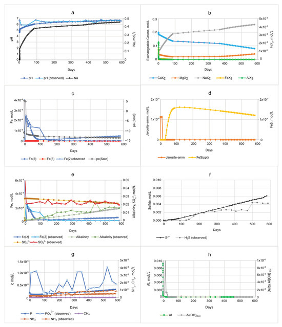
Figure 4.
Simulated pH and concentrations of dissolved constituents during simulated resalination of diked, flooded (DF) Herring River sediments based on [4] microcosm experiments. Changes in porewater chemistry as seawater passes through the column are shown in plots for (a) pH and Na; (b) exchangeable cations; (c) Fe and pe (Sato 1960); (d) jarosite-amm and FeS minerals; (e) Fe(II), SO42−, and alkalinity; (f) H2S and S2−; (g) PO43−, NH3, and CH4; and (h) Al and delta Al(OH)3(a).
The PHREEQC model calibrated to the [4] experiment data shows that seawater passes through the DF sediment column after about 8 h, as observed by Na+ concentrations and exchangeable cations (Figure 4a,b and Table S3). The DO initially present in seawater is immediately reduced after reacting with DF sediments that contain abundant SOM, Fe(II), and S2−, and Fe(II) increases sharply in the first 9 h (Figure 4c). The increasing front of dissolved solids concentration is accompanied by a brief decrease in pH as hydrogen ions (H+), Fe(II), and other cations are desorbed from sediments, and a small amount of jarosite-amm is dissolved (Figure 4a–d). The pe (Sato) in porewater peaks from 11 h to 14 days, before decreasing again as dissolved Fe(II) begins to increase. The desorption and exchange of Na+ for exchangeable cations including FeX2 (Equation (10)) and HX results in an initial Fe(II) concentration peak at 0.4 days (Figure 4c). Dissolved Fe(II) in porewater increases again and peaks at 3.4 µmol/L at 15 days in response to the reductive dissolution of jarosite-amm (Equation (9); Figure 4c,d). Once jarosite-amm is depleted after 10 days, SO42− reduction begins and S2− is generated after 14 days (Figure 4d–f; SM Table S3). The pH and alkalinity increase with the introduction of alkaline, SO42−-rich seawater and the generation of alkalinity from SOM oxidation coupled to Fe(III) mineral reduction and SO42− reduction (Equations (2) and (3); Figure 4d,e). As the concentration of SO42− is reduced, S2− increases, reacts with dissolved Fe(II), and begins to form FeS at about 30 days (Figure 4d,f). FeS mineral precipitation peaks after 118 days, then begins to dissolve after 149 days with the decreasing concentration of dissolved Fe(II) (Figure 4d,e).
Both alkalinity and NH4+ concentrations increase steadily throughout the DF sediment column simulation, along with a steady decrease in SO42−; this is consistent with SO42− reduction coupled to SOM oxidation (Figure 4e,g). Much of the total NH3 increase (includes both the NH4+ + NH3 forms) observed in the DF column experiments seems to result from the weathering of jarosite-amm and degradation of SOM rather than strictly desorption as surmised by [4]. NH4+ is the dominant and least toxic form of total NH3 in the moderately acidic DF porewater throughout most of the simulation. NH3 is the most toxic form to aquatic life and, at elevated pH, dominates over the ionized form, NH4+. Although P is commonly considered the “limiting nutrient” in freshwater ecosystems, it is generally not limiting in estuarine environments unless N inputs are sufficient, in which case PO43− inputs can cause eutrophication and harmful algal growth [68]. Phosphorus concentrations (nearly all in the form of PO43−) were less than 0.002 mmol/L as P at the beginning of the simulation and steadily increased after about 80 days, reaching 0.003 mmol/L after 582 days (Figure 4g).
Simulated Al concentrations peak sharply after 8 h as a result of desorption, to 15 mmol/L during the onset of salination, along with the precipitation of a small amount of Al(OH)3(a) (1.1 mmol/L) (Figure 4a,h). By 12 h, the Al peak drops to 0.62 mmol/L and gradually declines to 0.095 mmol/L by about 180 days (SM Table S3).
3.1.2. Biogeochemical Model of Diked, Drained (DD) Sediments
DD sediments have abundant Fe(III) minerals from the oxidation of FeS minerals, and so Fe(III)-reducing conditions prevail below the upper sediments that are subaerially exposed. The geochemical model of DD sediments includes SOM, the equilibrium phases jarosite-amm, FeS, and Al(OH)3(a), and exchangeable Fe(II), NH4+, and PO43− (SM Table S1b). The presence of Fe(III) and SO42− in these sediments (products of FeS oxidation) provides electron acceptors for Fe(III) reduction and SO42− reduction coupled to the oxidation of SOM. The responses of pH and solute concentrations to salination of DD sediments are shown in Figure 5, and the PHREEQC output file and more detailed (shorter time interval) plots are provided in SM Table S4.

Figure 5.
Simulated, and in some cases observed, pH and concentrations of dissolved constituents during simulated resalination of a diked, drained (DD) Herring River sediment column based on Portnoy and Giblin [4] microcosm experiments. Changes in porewater chemistry as seawater passes through the column are shown in plots for (a) pH and Na; (b) exchangeable cations; (c) Fe and pe [69]; (d) jarosite-amm and FeS minerals; (e) Fe(II), SO42−, and alkalinity; (f) H2S and S2−; (g) PO43−, NH3, and CH4, and (h) Al and delta Al(OH)3(a).

The simulated pH is very low (<4.3) at the beginning of the simulation because of the acidity produced from Fe sulfide oxidation and desorption of cations including H+ and Fe(II) (Figure 5a–c). Jarosite-amm was included as an equilibrium phase that varied with depth (SM Table S1b) to best match the Fe(II) concentration observed by Portnoy and Giblin [4]. After about 77 days of salination, the pH rises above 5 and alkalinity continues to increase, both from the high alkalinity in seawater and from the oxidation of SOM coupled to SO42− and Fe(III) reduction (Figure 5a–e; SM Table S4). At the beginning of the simulation, DO decreases to low concentrations after reacting with DD sediments that contain SOM, Fe(II), and S2− (SM Table S4). The jarosite-amm is depleted in 126 days, at which point the pe(Sato) drops to −12.6, SO42− reduction becomes the dominant electron-accepting process, and S2− begins reacting with dissolved Fe(II) to form FeS minerals (Figure 5c,d). FeS minerals stop forming at 583 days because Fe(II) concentrations are depleted. Because FeS is no longer forming, S2− concentrations sharply increase after 578 days.
Total NH3 concentrations are much higher in DD sediments than in DF sediments, which demonstrates the greater degradation rates of SOM, the greater abundance of jarosite-amm, and the acidic soils that allow for more sorbed NH4+ (Figure 5e,g). Simulated NH3 concentrations in porewater are similar to those observed in the Portnoy and Giblin [4] column experiments, ranging as high as 7.1 mmol/L (99 mg/L as N). PO43−-P concentrations are initially much higher (up to 0.12 mmol/L) in the DD sediment cores than in the DF cores (0.0019 mmol/L), probably due to the large sorbed fraction on the Fe oxides (jarosite-amm) in the DD cores that is released with reductive dissolution of jarosite-amm; PO43−-P concentrations decreased to 0.006 mmol/L once the Fe oxide was depleted. Simulated inorganic PO43−-P concentrations are initially higher than those observed in the Portnoy and Giblin [4] column experiments but decrease to background levels, contrary to measured inorganic PO43−-P concentrations in the experiment that increased to 0.15 mmol/L. This discrepancy may result from an Fe(III) phosphate mineral, such as vivianite, that is present in DF sediments but was not accounted for as an equilibrium phase in the model input. In acid SO42− soils, Krairapanond, et al. [70] found that PO43− sorption was mostly associated with Fe oxides and secondarily with Al oxides. In summary, smaller amounts of NH4+, PO43−, and Fe(II) were mobilized from the DF sediments as compared to the DD, because (1) less NH4+ was sorbed to these sediments, and (2) dissolved Fe(II) mobilized by seawater was precipitated as Fe sulfide minerals. CH4 concentrations increased rapidly at 560 days with the absence of preferred electron acceptors O2, Fe(III), and SO42−.
Al concentrations increase significantly, from 0.09 mmol/L to briefly peak at 200 mmol/L after 7 h of salination (SM Table S4), then gradually decline to 0.59 mmol/L after 79 days, below the original concentration (Figure 5h). A large amount of dissolved Al (244 mmol/L) is exchanged or desorbed off the acidic sediments during the first 88 days and some of this Al (1.4 mmol/L) is precipitated as Al(OH)3(a). Portnoy and Giblin [4] observed a 6-fold increase in porewater Al after salination that was attributed to cation exchange in the acidic Herring River marsh sediments.
3.1.3. Comparison of DF and DD Models
The simulated microcosm model results for DF and DD marsh sediments reflect the differing depositional environments and biogeochemistry of the two soil types and their response to salination (Table 5). DF sediments are freshwater-submerged, organic-matter rich, and methanogenic, and they have low amounts of Fe and SO42− due to more reducing conditions and sequestration by Fe sulfide minerals. The DD sediments, on the other hand, have abundant Fe(III) minerals from the oxidation of FeS minerals, and so Fe(III)-reducing conditions prevail below the upper sediments that are subaerially exposed. Porewater affected by seawater emerges from DF and DD sediments after about 8 h (Tables S3 and S4). Salination of both of these end-member sediments results in the mobilization of metals, nutrients, and DIC by desorption and the degradation of SOM.
Table 5.
Characteristics of sediments and water in diked salt marshes on Cape Cod, MA, before tidal restoration [4,58] and after microcosm simulations.
The pH in both DF and DD sediment porewater drops initially from the mobilization of acidity, then rises from buffering by seawater and the oxidation of SOM coupled to electron acceptors (Figure 4a–e and Figure 5a–e). The simulated pH is lower in DD (as low as 4.2 pH) compared to DF sediments (as low as 4.7 pH), for the first 85 days of the simulation, primarily because of the acid-sulfate DD soils (Figure 4d and Figure 5d).
The DO in DF porewater is rapidly reduced as seawater reacts with sediments that contain abundant reductants (SOM, Fe(II), and S2−). In DD sediments, however, the presence of Fe(III) minerals and SO42− provides suitable conditions for Fe(III) reduction and SO42− reduction below the upper sediments. The greater SOM degradation rates estimated for DD sediments result from the energetically more favorable reductive dissolution of Fe(III) minerals (jarosite-amm) compared to DF sediments, where SO42− reduction becomes the primary redox process (Table 2). The higher alkalinity generated from DD porewater is consistent with the greater DD SOM mineralization rates from the microcosm model fittings, compared to the more reduced DF sediments (Table 2; Figure 4e and Figure 5e).
All Fe forms are much higher in DD sediments compared to DF sediments. Dissolved Fe concentrations in DD sediments peak at 0.24 mmol/L after 15 days, then decline to 0.01 mmol/L by 118 days as jarosite-amm is depleted (Figure 4c). DF porewater concentrations then rise gradually again as Fe sulfide minerals dissolve and reach 3.4 mmol/L by the end of the simulation, 578 days. Dissolved Fe concentrations in DD porewater are much higher, as a result of the oxic conditions and the abundance of oxidized pyrite. Dissolved Fe in DD porewater peaks at 46 mmol/L at 385 days (desorption and reductive dissolution of jarosite-amm), then are depleted by 583 days as Fe(II) reacts with S2− to form FeS/ FeS2 (Figure 5c). The S−2 porewater concentrations in both modeled sediments are initially very low (Figure 4f and Figure 5f). The S−2 in DF porewater gradually increases to 6.1 mmol/L by the end of the simulation. The S−2 concentration in the DD porewater sharply increases to 28 mmol/L by 578 days and coincides with the decrease in dissolved Fe(II) and the slowing formation of FeS. Although DF sediments are more reduced throughout much of the simulations, DD sediments become methanogenic near the end, and CH4 concentrations increase rapidly to peak at 2.8 mmol/L at 578 days.
Aside from sorbed Fe, jarosite-amm and FeS are the major Fe forms simulated in the microcosm models. The jarosite-amm in DF sediments peaks at 0.1 mmol/L after 12 h of salination but is depleted through reductive dissolution by 10 days. The jarosite-amm in DD sediments is present initially at 25 mmol/L and is depleted through reductive dissolution by 126 days (Figure 4d and Figure 5d). This is important because the energetically more favorable reductive dissolution of jarosite-amm in DD sediments compared to the Fe(III)-poor DF sediments results in greater C degradation rates. S2− concentrations also are lower in DD sediments (Figure 4g and Figure 5g), due to the greater amount of FeS mineral being formed (Figure 4d and Figure 5d). For DF sediments, FeS mineral precipitation peaks after 118 days (coincident with lower dissolved Fe(II)), then begins to dissolve, reaching 0.12 mmol/L after 580 days (Figure 4d,e). For DD sediments, FeS minerals begin forming later, after 118 days, and reach 0.38 mmol/L by the end of the simulation at 589 days (Figure 5b).
Dissolved concentrations of NH4+ and P are mobilized from marsh sediments by the accelerated organic decomposition and also by desorption, as brought on by seawater restoration. Porewater NH4+ concentrations in DF sediments are very low initially and gradually increase to 0.52 µmol/L by 580 days. NH4+ concentrations in DD porewater rise more rapidly, from 0.62 to 5.7 mmol/L by the end of the simulation. Portnoy and Giblin [4] found the NH4+ adsorbed on silts and clays of the aerated DD soils. Porewater PO43− concentrations were low in DF sediments and gradually increased to 3.3 µmol/L by 580 days. Dissolved PO43− in DD sediments was high initially (12.5 mmol/L), decreased and peaked again after 5 days, then dropped below 10 µmol/L for the remainder of the simulation. PO43− in DD sediments was found to be likely associated with abundant Fe and Al oxides [4].
Simulated Al concentrations in porewater peak sharply within 7 or 8 h of salination from both DF and DD sediments. Al concentrations in DD porewaters were much higher (up to 200 mmol/L) and remained over 100 mmol/L for 5 h, until gradually declining to 0.59 mmol/L by 80 days.
3.2. Basecase Simulations of Seawater Flooding in Diked Marsh Sediments
The biogeochemical responses of DF and DD porewaters to salination in the 12 yr run basecase models (Figure 6; SM Tables S6 and S7) are generally similar but extended over a longer period compared to solute responses of the microcosm experiment simulations, which began with a high rate of flushing in the first 12 h (Table 1). Because the initially high flow rate was not used in the basecase models, these simulations can be used as a more conservative estimate of porewater movement through low permeability marsh sediments. Besides using jarosite-amm, additional Fe(III) source minerals were used in a sensitivity analysis to assess the effects of their varying reactivities and solubilities on simulated porewater biogeochemistry (SM Tables S2a–j). In addition to jarosite-amm (log k = −19.02), other Fe(III) oxide minerals include schwertmannite (another Fe(III) oxyhydroxy-sulfate mineral, log k = 2.25), Fe(OH)2(a) (log k = 4.89), and goethite (log k = −1.0) [71] that were included in separate simulations (Section 3.1.2). In addition, jarosite-amm was simulated at a higher initial concentration (0.11 mol/L), an order of magnitude greater than was used in the basecase scenarios. Finally, extended basecase simulations that were run for over 100 yrs provide improved long-term understanding of conditions and processes that affect constituents of concern.
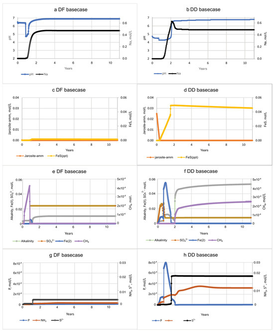
Figure 6.
The pH and solute concentrations during the basecase model salination simulations of diked, flooded (DF) and diked, drained (DD) sediments. Changes in porewater chemistry as seawater passes through the columns are shown in plots for pH (a,b) and Na; jarosite-amm and FeS minerals (c,d); alkalinity, Fe(II), SO42−, and CH4 (e,f); and PO43−, NH3; and S2− (g,h).
The porewater pH in the basecase models during the first 2 yrs was acidic in both cores, dipping briefly to 4.8 with DF porewater, and remaining below pH 5 with DD porewater for over 2 yrs. The pH of DD porewater was much lower at the beginning of the simulation than the DF sediment because of the acidity produced by Fe sulfide oxidation and cation exchange that mobilizes cations including H+ and Fe(II). The low Fe(II) concentration in the DF sediment (Figure 6c) is consistent with the relatively small amount of jarosite-amm dissolution (Figure 6d–f), whereas the more abundant Fe(III) source (jarosite-amm) in the DD sediment resulted in accompanying increases in Fe(II), as well as NH3 and PO43− concentrations (Figure 6e–h). Alkalinity concentrations in the basecase simulations increased up to 0.01 mol/L in DF porewater and up to 0.05 mol/L in DD porewater after 5 yrs (Figure 6e,f) and demonstrate the greater degradation of organic C from Fe(III) reduction, SO42− reduction, and methanogenesis.
Concentrations of Al species increase with the drop in pH during both microcosm and basecase simulations (Figure 7 and Figure 8; SM Tables S3, S4, S6 and S7). Al concentrations are dominated by Al+3, AlSO4+, and AlOH+2 at both DF and DD sites. Al concentrations peaks much earlier in the microcosm simulations, because of the relatively high rate of flushing used in the beginning of the experiments. For the DF microcosm simulation, Al peaks only briefly at 0.36 days, coincident with the 3.6- hr dip in pH from 6.7 to 4.6, before decreasing to background levels by 0.5 days (Figure 7a). Because of the sustained acidic conditions in DD porewater, concentrations of Al species are much higher (0.2 mol/L) and extend over a longer period (80 days) compared to the DF sites (Figure 7; SM Tables S3 and S4). For the basecase simulations, concentrations of Al+3, AlSO4+, and AlOH+2 also dominate the Al species. Al+3 has the highest concentration and AlOH+2, the most toxic species, has the lowest concentration. Al in DF porewater peaks between 319 days to 425 days and reaches 0.01 mol/L (Figure 8a; SM Table S6). The DD microcosm simulation has the same relative concentrations of Al species as the DD basecase simulation, peaking at 0.19 mol/L with a coincident drop in pH to 4.2 at 315 days. Al concentration does not decline until the rise of pH after 2 yrs (Figure 8b; SM Table S7).
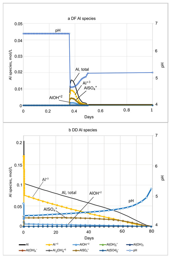
Figure 7.
Plots showing the PHREEQC Al species concentrations and pH during microcosm experiment simulations of seawater movement through (a) diked, flooded (DF) sediments and (b) diked, drained (DD) sediments based on Portnoy and Giblin [4] microcosm experiments. Assumed Al solubility control by Al(OH)3(a).
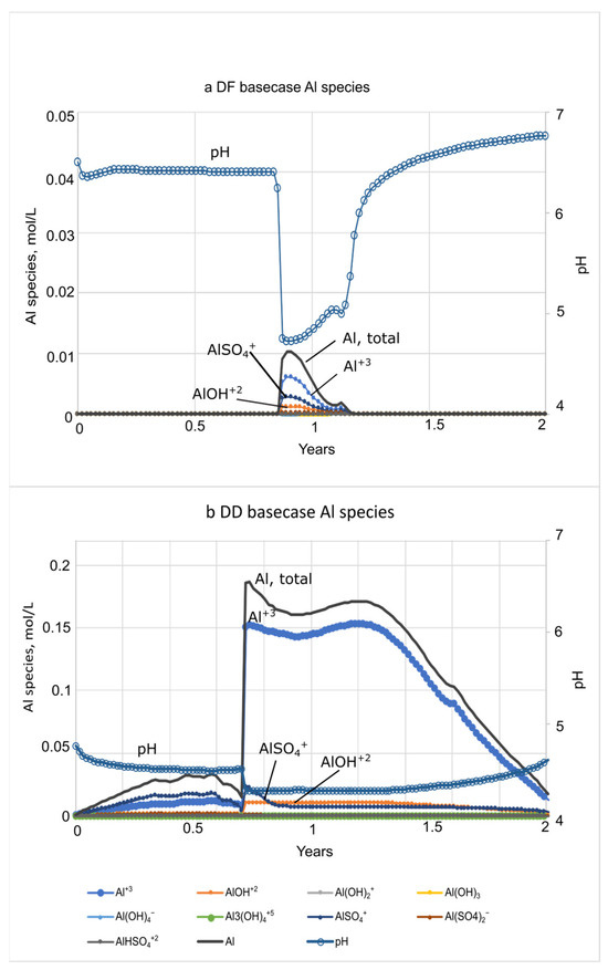
Figure 8.
Plots showing PHREEQC Al species concentrations and pH during basecase simulations of seawater movement through (a) diked, flooded (DF) sediments and (b) diked, drained (DD) sediments. Assumed Al solubility control by Al(OH)3(a).
Extended (100 yr) basecase simulations show that pH (6.9, 6.8) and the pe(Sato) (−13.6, −13.2) in DF and DD sediment porewaters are very similar after 100 yrs. Whereas dissolved Fe in DF porewater is zero after depletion of Fe sources, DD porewater had 0.64 mmol/L from the oxidative dissolution of FeS. The S2− concentrations in the more reduced DF sediments reach a stable concentration of 0.0034 mol/L after a year of resalination; after 1.6 yrs, S2− concentrations in DD porewater increased as Fe(III) was depleted and FeS minerals stop forming and begin to dissolve, but slowly, and they still have concentrations of 0.04 mol/L at the end of the 100 yr simulations (SM Table S10b). Alternatively, S2− in DD sediments are higher (0.02 mol/L) but decrease to near zero by 19 yrs (SM Table S10a,b). Simulated FeS in DF marsh sediments is much lower in abundance (by 15×) than that of DD, oxidizing more rapidly, and is depleted by 33 yrs (SM Table S10a). NH3 concentrations in DF porewater increase at about 9 months, reach 1 mol/L after 4 yrs, and remain steady for 100 yrs. NH3 concentrations in DD porewater reach 0.078 mol/L at just under 5 yrs and decline with the gradual rise in pH and the depletion of jarosite-amm to a negligible concentration after 24 yrs (SM Table S10b).
The 12 yr basecase scenario was then modified in a sensitivity analysis to assess the effects of varying types and amounts of Fe(III) source minerals on pH and solute concentrations. The dissolution of Fe(III) hydroxide minerals varied; the more soluble Fe(OH)2(a), schwertmannite, and goethite were generally depleted earlier than jarosite-amm (Figure 9a,b; SM Tables S8a–d and S9a–d). All of the Fe(III) sources in the simulations were reduced by organic C oxidation and not by S2− because they were depleted by the time S2− concentrations increased after seawater was introduced and SO42− reduction became dominant. Fe(III) minerals in DF sediments are much less abundant than in DD sediments and are generally depleted within 6 months, with the exception of the simulation including high (10x) jarosite-amm, which remained until about 7.7 yrs. Porewater concentrations of Fe(II) in DF sediments are also low, 0.036 mol/L for 10× jarosite-amm, compared to 0.22 mol/L in DD sediments (Figure 9c,d; SM Table S8d). FeS mineral precipitation increases with the availability of Fe(II) from Fe(III) mineral dissolution (Figure 9c–f) and S2− (reduced from SO42− in seawater; SM Tables S8 and S9). Although jarosite-amm has a lower solubility than the other Fe(III) sources, simulations indicate that Fe(II) concentrations peak higher and last longer (Figure 9c,d). Once the Fe(III) minerals are depleted, S2− concentrations increase and remain high as SO42− reduction becomes the dominant electron acceptor for organic C degradation. The amount of FeS mineral in DF sediments remains steady or slightly declining over the 12 yr simulation, higher in jarosite-amm than in simulations with other Fe(III) minerals (Figure 9e,f; SM Table S8). The high (×10) concentration of jarosite-amm used in simulations also results in higher pH (greater than 8) compared to the default concentration and reflects the consumption of acidity during both Fe(III) mineral dissolution and FeS precipitation (SM Tables S8d and S9d).
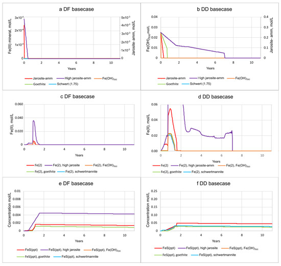
Figure 9.
The mineral and porewater concentrations during basecase simulations with varying types (and jarosite-amm strength) of Fe(III) source minerals, including jarosite-amm, 10× amount of jarosite-amm, Fe(OH)3(a), schwertmannite, and goethite. Changes in porewater chemistry as seawater passes through the sediments are shown in plots for Fe(III) mineral (a,b); Fe2+ or Fe(II) (c,d); and FeS minerals (e,f) for diked, flooded (DF) and diked, drained (DD) sediments, respectively.
3.3. Biogeochemical Implications of Seawater Restoration
The microcosm experiment models and the basecase models can be used to better understand the biogeochemical implications of seawater restoration on the Herring River and Wellfleet Harbor by incorporating speciation for constituents of concern (Al), varying the Fe(III) hydroxide source and strength, varying the flow rate, and varying the time interval. These models could also be applied to other freshwater marshes along coastal areas that are vulnerable to changing climatic conditions and sea-level rise. Aquatic organisms are adversely affected by low pH, suboxic or anoxic conditions, and high concentrations of dissolved Fe, S2−, and Al. Fluxes of solutes such as NH4+ and PO43− to coastal water could cause eutrophication and hypoxia.
The sediment column salination simulations (and the column experiments) are a 1-D simplification of the actual field conditions that contain temporal and spatial variability associated with the seasons, tidal effects, precipitation, interaction with groundwater, and the heterogeneities in biogeochemistry, sediment texture, SOM content, bioturbation, and flow rates. For example, SOM degradation rates and organo-metallic complexation are likely to be higher during warm seasons [48,72]; Al toxicity increases with temperature; the acidity and concentrations of nutrients, Fe, S2−, and Al vary with SOM content [48,73]; and nutrient fluxes will vary with tide amplitude because of varying dilution by seawater. These results can be used to determine and help isolate biogeochemical processes, estimate rates, and determine potential concerns for aquatic life. In particular, the models can improve understanding of the biogeochemical processes, the interaction of constituents of concern with pH, redox, and complexation, and the general timing and sequence of the contaminant releases and reactions. Future work could include coupling the PHREEC models with two- or three-dimensional groundwater flow and solute transport models to simulate progressive mixing of tidally varying saltwater into the freshwater marsh sediments.
Several constituents derived from the DF and DD marsh sediments are a concern to both freshwater and saltwater aquatic health in the Herring River and Wellfleet Harbor (SM Table S5). Since 2021, biogeochemical conditions similar to those expected during marsh restoration have been observed episodically at Herring River monitoring stations at Duck Harbor due to overwash that carries saltwater over the dune crest into the Herring River watershed (Figure 2; Timothy Smith, National Park Service written communication, 2023). These overwash events, which are observed almost monthly during spring tides, have caused a significant die off of vegetation and have resulted in low pH and elevated concentrations of Fe(II) and NH4+ in water samples and/or continuous monitors in the Herring River (Sophia Fox, National Park Service written communication, 2023).
In the microcosm experiment simulations for DF sediments, pH was as low as 4.7 after about 8 h, which is well under the freshwater-quality criteria range (6.5–9), until waters became saline at 8.7 h. At 8.7 h and later, the pH was well under the acceptable saltwater-quality criteria range (6.5–8.5) and remained so until about 400 days; pH varying outside those ranges approaches the lethal limits of some species [74] (SM Table S5). The basecase models showed delayed changes in solutes, and the pH drop began over 300 days into the simulation.
Dissolved Fe in microcosm simulations were below the freshwater health criterion of 1000 µg/L for both DF and DD cores. Although there are no saltwater health criteria for Fe [54], Fe can be detrimental to the health of fish, invertebrates, and periphyton and can cause oxidative injury to various organs and physical damage to the gills [75,76]. Fe concentrations were well over 5 mmol/L (300 µg/L) in the DD core after 10 h until near the end of the simulation (SM Table S5).
SM Table S5 shows both the EPA’s 2018 and the 1988 Al guidance criteria for freshwaters [74,77]. The early peak in Al concentrations for the DF core is above EPA’s 2018 guidance but below the Al guidance range that considers pH and hardness [54]. Al concentrations in saline water exceed 24 μg/L from 8.5 h until 58 days of the DF microcosm experiment simulation. For DD sediments, the pH and temperature affect the proportion of the neutral NH3 species and therefore are used to determine the freshwater aquatic criteria for NH3. There are two exceedances of the total NH3 saltwater aquatic criteria for the DD microcosm simulation, 19 mg/L (1.4 mmol/L) and 16 mg/L (1.1 mmol/L) near the end of the 589 day simulation after pH had risen and NH3 was more dominant (SM Table S5) [55,78]. Freshwater criteria for NH3 are pH, temperature, and life-stage dependent, whereas those criteria for saltwater are only pH and temperature dependent.
Al is an example of a constituent of concern that can vary significantly in porewater with biogeochemical conditions during seawater restoration, as illustrated in differences between the microcosm experiment models and the basecase models (Figure 4, Figure 5 and Figure 6). High Al concentrations are most common in freshwater because of the greater solubility of Al under the often acidic (<7 pH) conditions. Al toxicity is reduced by increases in cations including Ca2+ and Mg2+ that compete with Al3+ for uptake by aquatic organisms [79,80] and can be measured as total hardness [54]. Al toxicity also decreases when Al complexes with dissolved organic carbon (DOC), thereby reducing the bioavailability to aquatic organisms [79,81,82]. Al concentration, speciation, and toxicity in estuaries varies with pH and with temperature, DOC concentrations, and base cations, including Ca and Mg. Al minerals are moderately soluble below pH 5, with toxicity increasing up to a pH of about 6.0 (at 25 °C), at which point amorphous Al(OH)3(a) or gibbsite [83,84] dissolve and aqueous Al peaks. Al species were included in the microcosm and basecase salination models of the Herring River sediment porewater (Figure 7 and Figure 8; Tables S3, S4, S6 and S7). The toxic Al species Al(OH)2+ dominates between pH 5 and 6 [83]. Concentrations of Al(OH)2+ exceeded the freshwater acute Al value (varies with temperature, pH, DOC, and hardness) in DD sediments until saline conditions ensued after 10 days, and thereafter exceeded the chronic Al value (24 µg/L; [85]) for more than 500 days (SM Table S5). With the basecase models, Al concentrations increased at both sites with the drop in pH, peaking after about one year, and consisted mostly of Al+3, AlSO4+, and AlOH+2 (Figure 8). As mentioned previously, Al toxicity decreases when Al complexes with DOC, which varies seasonally, although DOC complexation was not simulated here. In addition, cold water will have a greater proportion of toxic species at higher pH values than warm water [86], although the temperature effects on speciation was not simulated. As a result of these factors, seasonality could have important effects on Al toxicity in the Herring River, and salination during colder months could be problematic to aquatic life.
Another potentially important factor not studied here but directly relevant to post restoration biogeochemical conditions is the compaction of sediments resulting from accelerated aeration, organic decomposition, and subsidence that occurs following seawater restoration [4,5]. Portnoy and Giblin [4] observed 6–8 cm of subsidence in the DF microcosm cores. The diking has also blocked the flood-tide sediment source to the marsh and led to further subsidence [5]. Because of this subsidence and exacerbated by sea-level rise, tidal restoration can lead to a greater extent of seawater inundation onto marsh sediments compared to natural conditions [87,88]. The prolonged seawater flooding resulting from this subsidence could therefore lead to a greater extent of desorption and redox chemistry changes, and larger pulses of acidity, metals, and nutrients that are harmful to the aquatic ecosystem, as described in this section.
The persistence of FeS (and presumably also FeS2) in extended simulations, particularly in DD sediments, reflects the tidally flooded conditions common to normal salt marsh soils in which Fe, S, and acidity are generally immobilized. Burton et al. [16] found that tidal reflooding of wetland acid SO42− soils resulted in enrichment of Fe2+ and SO42− and pyrite reformation within the subtidal zone and did not result in rapid restoration. However, extended simulations of Herring River sediments show that pH increases and concentrations of most solutes in DF and DD sediments converge over time (Table S10a,b). Simulated concentrations of S2− in DD porewater remain elevated for several years (Figure 6) before decreasing to near zero after almost 20 yrs (SM Table S10a,b); S2− toxicity is less of a concern in DD sediments because the high concentrations of Fe(II) mobilized by seawater precipitate sulfides. S2− toxicity can cause reduced plant uptake [89], and various fish species are sensitive to un-ionized H2S [74].
These biogeochemical modeling simulations illustrate the complexities and improve understanding of how diked or otherwise freshwater wetlands and their globally important carbon reservoirs respond biogeochemically to dike removal and sea-level rise. Organic C degradation and its effect on biogeochemical cycling of Fe, S, CH4, N, and P is intimately connected to microbe–soil–plant interactions in sediments [90]. Both the DF and DD sediments have NH4+ sorbed on silts and clays and PO43− likely associated with abundant Fe and Al oxides (Dent 1986). As shown in the model simulations, salination has the potential to mobilize a large pulse of NH4+, PO43−, H+, and Fe(II) (as already observed in part at the Duck Harbor overwash area on the Herring River; Figure 2), as well as potentially toxic levels of Al. The large amount of S2− stored in these diked sediments, even the drained aerobic sediments [62], can result in a sharp increase in acidity but will eventually moderate by seawater buffering. Therefore, gradual restoration and careful monitoring of tidal restorations in diked wetlands could help mitigate the immediate negative effects of biogeochemical changes associated with restoration activities. With the resalination of diked coastal wetlands such as the Herring River, SO42− reducers will likely overtake methanogens in SOM decomposition, which increases thermodynamic energy yields and subsequently increases the turnover of N and P.
4. Summary and Conclusions
Biogeochemical models were developed and calibrated to greenhouse microcosm experiments that were conducted to assess the biogeochemical effects of seawater restoration on the historically diked Herring River marsh for diked, flooded (DF) sediments and diked, drained (DD) sediments by Portnoy and Giblin [4]. Models for 1-D reactive transport of solutes in these marsh sediment porewaters were developed using PHREEQC, matching the simulated solute curves with the results from Portnoy and Giblin [4] microcosm experiments. Basecase models were then modified from the microcosm experiment models to simulate salination over longer time periods using single flow velocities and varying Fe source mineral types and strength to better understand biogeochemical conditions.
The reintroduction of seawater to marsh sediments in the microcosm simulations showed flushing of acidic porewater with sometimes high concentrations of Fe2+, S2−, H+, NH3, and Al. The simulated microcosm model results for DF and DD marsh sediments reflect the differing depositional environments and biogeochemistry of the two soil types and their response to salination (Table 5). Desorption was significant, particularly in DD sediments, and simulated using both ion exchange and surface complexation reactions. The pH in both DF and DD sediment porewater drops initially from the mobilization of acidity, then rises from buffering by seawater and the oxidation of SOM coupled to electron acceptors. The simulated pH is lower in DD (as low as 4.2 pH) compared to DF sediments (as low as 4.7 pH), for the first 85 days of the simulation, primarily because of the acid sulfate DD soils. Simulated porewater pHs were at times below the acceptable freshwater- and (or) saltwater-quality criteria ranges for both sediment types.
Simulated redox conditions shifted quickly after the onset of salination; DF porewater shifted from methanogenic to SO42− reducing after 10 days. DD porewater quickly became Fe(III), reducing as a result of jarosite-amm dissolution. Potential to exceed aquatic criteria levels is greater for DD sediments because the acidic conditions generally allow for greater capacity to sorb Fe2+, S2−, NH3, and Al. NH3 was much higher in DD porewater than in DF sediments because of the greater degradation rates of the SOM and the acidic soils that allowed for more NH4+ sorption before salination. Al concentrations in DD porewater exceeded the 24 µg/L saltwater aquatic criteria [91] for DD sediments once the porewater became saline (10 h) and thereafter exceeded the chronic saltwater Al value (24 µg/L) for more than 500 days. Although Al and most metals would be much less soluble once seawater infiltrates marsh sediments and the pH increases, the toxic species Al(OH)2+ dominated the total Al concentrations under the initially acidic conditions and exceeded the USEPA freshwater acute Al level in DD sediment porewater.
The basecase simulations (run over 12 yrs) of DF and DD porewaters showed similar biogeochemical responses to salination as the microcosm simulations, but the lower flow rates represent a conservative flow estimate that might be observed in low permeability marsh sediments. These basecase reactive transport models, which are based on calibrated real-world diked marshes, allow simulations of varying flow and biogeochemical conditions, and speciation of contaminants such as Al. Jarosite-amm, a likely Fe(III) source in Herring River sediments, has a lower solubility than other possible Fe(III) sources [92] and simulations indicate that Fe(II) concentrations peaked later and longer than for Fe(OH)2(a), goethite, or schwertmannite.
Extended basecase simulations were run for over 100 yrs to provide long-term understanding of conditions and processes that affect constituents of concern. For example, S2− concentrations in the more reduced DF sediments reach a stable concentration of 0.0034 mol/L after a year of resalination, whereas S2− in DD sediments are higher (0.02 mol/L) but decrease to near zero by 19 yrs. Simulated FeS in DF marsh sediments was much lower in abundance (by 15×) than that of DD sediments, oxidized more rapidly, and was depleted by 33 yrs. NH3 concentrations in DF porewater increased rapidly at about 9 months, reached 1 mol/L after 4 yrs, and remained steady for 100 yrs. NH3 concentrations in DD porewater reached 0.078 mol/L at just under 5 yrs and declined to a negligible concentration after 24 yrs with the gradual rise in pH and the depletion of jarosite-amm.
This study was undertaken to help inform National Park Service staff on the level and duration of expected risk and the best strategies associated with dike opening. Although there is significant uncertainty in 1-D geochemical simulations, this study utilizes site-specific data that are common to data collected in other tide-restricted marsh systems worldwide that contain low pH and harmful or toxic levels of acidity, metals, and nutrients. In addition, these findings are consistent with recently observed spring tide overwash events at the Herring River that have led to locally acidic and Fe-fouled conditions. Future work could include coupling the PHREEQC models with two- or three-dimensional groundwater flow and solute transport models to simulate progressive mixing of tidally varying saltwater into the freshwater marsh sediments. These results can be used to help understand the general timing and sequence of the contaminant releases and reactions (including complexation, desorption, and degradation of SOM), and the potential risks to aquatic life.
Supplementary Materials
Geochemical modeling data and model calibration details that support the findings in this paper can be downloaded at https://www.mdpi.com/article/10.3390/soilsystems9030089/s1, SM File S1 contains the following tables [4,5,27,29,33,65,66,85,93,94,95,96]; Table S1a: Microcosm model input used to simulate resalination of diked, flooded (DF) sediment column, Herring River, Wellfleet, Massachusetts; Table S1b: Microcosm model input used to simulate resalination of diked, drained (DD) sediment column, Herring River, Wellfleet, Massachusetts; Table S2a: Basecase model input used to simulate resalination of diked, flooded sediments of the Herring River, Wellfleet, Massachusetts, over a 12-year period; Table S2b: Basecase model input used to simulate resalination of diked, drained sediments of the Herring River, Wellfleet Massachusetts, over a 12-year period; Table S2c: Basecase model input used to simulate resalination of diked, flooded sediments of the Herring River, Wellfleet Massachusetts, over a 12-year period, using Fe(OH)3(a) as the Fe(III) source; Table S2d: Basecase model input used to simulate resalination of diked, flooded sediments of the Herring River, Wellfleet Massachusetts, over a 12-year period, using goethite as the Fe(III) source; Table S2e: Basecase model input used to simulate resalination of diked, flooded sediments of the Herring River, Wellfleet Massachusetts, over a 12-year period, using schwertmannite (1.75) as the Fe(III) source; Table S2f: Basecase model input used to simulate resalination of diked, flooded sediments of the Herring River, Wellfleet Massachusetts, over a 12-year period, using a high concentration of ammonium jarosite as the Fe(III) source; Table S2g: Basecase model input used to simulate resalination of diked, drained sediments of the Herring River, Wellfleet Massachusetts, over a 12-year period, using Fe(OH)3(a) as the Fe(III) source; Table S2h: Basecase model input used to simulate resalination of diked, drained sediments of the Herring River, Wellfleet Massachusetts, over a 12-year period, using goethite as the Fe(III) source; Table S2i: Basecase model input used to simulate resalination of diked, drained sediments of the Herring River, Wellfleet Massachusetts, over a 12-year period, using schwertmannite (1.75) as the Fe(III) source; Table S2j: Basecase model input used to simulate resalination of diked, drained sediments of the Herring River, Wellfleet Massachusetts, over a 12-year period, using a high concentration of ammonium jarosite as the Fe(III) source; Table S2k: Basecase model input used to simulate resalination of diked, flooded sediments of the Herring River, Wellfleet, Massachusetts, over a 100-year period; Table S2l: Basecase model input used to simulate resalination of diked, drained sediments of the Herring River, Wellfleet Massachusetts, over a 100-year period; Table S3: PHREEQC selected output file and sediment porewater chemistry plots from model simulation representing microcosm experiments conducted for diked, flooded (DF) sediment column, Herring River, Wellfleet, Massachusetts; Table S4: PHREEQC selected output file and sediment porewater chemistry plots from model simulation representing microcosm experiments conducted for diked, drained (DD) sediment column, Herring River, Wellfleet, Massachusetts; Table S5: Porewater chemistry PHREEQC Herring River sediment model output and aquatic life water quality criteria for simulated pH and solute concentrations after salination of diked, flooded (DF) and diked, drained (DD) sediments based on microcosm models; Table S6: PHREEQC selected output file and sediment porewater chemistry plots for DF basecase model simulation for 12-year period; Table S7: PHREEQC selected output file and sediment porewater chemistry plots for DD basecase model simulation for 12-year period; Table S8a: PHREEQC selected output file and sediment porewater chemistry plots for DF basecase model simulation with Fe(OH)3(a) as the Fe(III) source mineral for 12-year period; Table S8b: PHREEQC selected output file and sediment porewater chemistry plots for DF basecase model simulation with goethite as the Fe(III) source mineral for 12-year period; Table S8c: PHREEQC selected output file and sediment porewater chemistry plots for DF basecase model simulation with schwertmannite as the Fe(III) source mineral for 12-year period; Table S8d: PHREEQC selected output file and sediment porewater chemistry plots for DF basecase model simulation with Fe(OH)3(a) as the Fe(III) source mineral for 12-year period; Table S9a: PHREEQC selected output file and sediment porewater chemistry plots for DF basecase model simulation with Fe(OH)3(a) as the Fe(III) source mineral for 12-year period; Table S9b: PHREEQC selected output file and sediment porewater chemistry plots for DF basecase model simulation with goethite as the Fe(III) source mineral for 12-year period; Table S9c: PHREEQC selected output file and sediment porewater chemistry plots for DF basecase model simulation with schwertmannite as the Fe(III) source mineral for 12-year period; Table S9d: PHREEQC selected output file and sediment porewater chemistry plots for DF basecase model simulation with Fe(OH)3(a) as the Fe(III) source mineral for 12-year period; Table S10a: PHREEQC selected output file and sediment porewater chemistry plots for DF basecase model simulation for 100-year period; Table S10b: PHREEQC selected output file and sediment porewater chemistry plots for DD basecase model simulation for 100-year period. SM File S2 describes the calibration of microcosm models [4,5,33,64,66,96,97].
Funding
This research was cooperatively funded by the National Park Service. Any use of trade, firm, or product names is for descriptive purposes only and does not imply endorsement by the U.S. government.
Data Availability Statement
An associated USGS data release [33] is available.
Acknowledgments
The author is grateful for the support received from several people who contributed to the successful completion of this study. Timothy Smith and Sophia Fox at the Cape Cod National Seashore (National Park Service, or NPS) provided logistical support and provided water-quality condition updates based on monitoring at the Herring River. This article benefited greatly from the colleague reviews by Kevin Kroeger (USGS), and John Portnoy (NPS, retired), and anonymous journal reviewers.
Conflicts of Interest
The author has no conflicts of interest, including financial interests, associated with this work. Experimental data from Portnoy and Giblin [4,5] used in this article are referenced.
Appendix A. Previous Marsh Sediment Microcosm Experiments
The previously conducted Portnoy and Giblin [4] microcosm column experiments consisted of columns filled with DF and DD marsh sediments in which saltwater was introduced at the column top and withdrawn and monitored from a sampling port at the bottom (Figure 3). The cores were incubated for 21 months in an unheated greenhouse so that seasonal light and temperature cycles would be natural, and initial and final conditions in the solid phase and pore water chemistry were measured monthly. The DF marsh sediment core was obtained from an impounded portion of the North Sunken Meadow salt marsh in Eastham, MA (Figure 1) where diking and impoundment have resulted in the accumulation over the original salt marsh of ~27 cm of freshwater wetland peat near the surface; however, the DF marsh has retained reduced marine deposits below 30 cm that include pyrite [4,5]. The DD marsh sediment core was obtained at Herring River, Wellfleet, MA (Figure 1); constant drainage and aeration of the top 20 cm of sediment resulted in the decomposition of SOM and oxidation of pyrite and caused about 90 cm of subsidence [4]. The porewater chemistry from the DF and DD cores was also compared with that from a natural core (NA) collected from a natural, undiked salt marsh at North Sunken Meadow [5].
The DF and DD sediment cores were initially flushed with 10 L of water to exchange the freshwater for saltwater over a 12 h period. Subsequent flow rates from saltwater additions to make up for sampling water and evaporation were 1 to 2 orders of magnitude slower. The same amounts of saltwater were added in both the DD and DF cores; because of different porosities in DD and DF, flow rates varied between the cores (Table 1). By introducing water and KCl to DD and DF marsh sediment cores, Portnoy and Giblin [4] showed that large amounts of exchangeable Fe2+ (FeX2) were sorbed on DD sediment and large amounts of NH4+ were sorbed on DD and DF sediments. Fe(II) concentrations measured in cores were roughly constant with depth in DF and natural (NA) cores but increased with depth in DD cores [5]. During a pretreatment period from October 1992 to late January 1993, cores were flushed monthly with 1 L of fresh porewater that was prepared to chemically match water collected and analyzed over the previous 2 years from the Truro National Atmospheric Deposition site (Figure 1) [98,99].
The porewater pH and solute concentrations changed over time and distance in the greenhouse microcosm cores as the solution reacted with the core solids [Figure 3 and Figure 4]. After filling with saltwater, the oxygen was quickly depleted, followed by nitrate (likely at low concentrations), and then Fe(III) was depleted. The microbially mediated oxidation of SOM in the sediments coupled to the reduction of Fe(III) and SO42− caused increased concentrations of dissolved Fe(II) and S2− (Equations (2) and (3)).
The DF sediment porewater pH declined initially, then recovered to starting levels and remained stable throughout [4]. Alkalinity and S2− increased 10-fold between January salination and August 1993; Fe(II) increased about 50-fold by March but was depleted by July. Soluble S2− increased to high concentrations (4.5 mmol/L), and Fe(II) increased moderately in the DF sediments (up to 240 µmol/L in 4 months), then decreased to very low levels (5 µmol/L) as mackinawite or pyrite precipitated (Equation (5)) [4]. NH3 concentrations consistently increased after salination and dissolved inorganic phosphorus (P) increased by 2 to 10 times from initial concentrations [4].
The initial pH of the DD sediment porewater was low (4.0) and dissolved Fe(II) was high (10 mmol/L), indicating oxidized Fe sulfide minerals in the sediment [4]. Fe(II) increased to very high levels (60 mmol/L) by 7 months after salination and then decreased to near the initial concentration (10 mmol/L). Alkalinity increased to almost 40 mmol/L with the influx of seawater and degradation of SOM. NH3 concentrations increased 60-fold to over 6 mmol/L after salination, mostly from desorption, and dissolved inorganic P concentrations increased more than 20 times from July 1993 to October 1994 [4]. Dissolved Al, derived from clay minerals, increased by 6 times after salination and likely complexed with PO43− [4].
References
- Soukup, M.A.; Portnoy, J.W. Impacts from mosquito control-induced sulphur mobilization in a Cape Cod estuary. Environ. Conserv. 1986, 13, 47–50. [Google Scholar] [CrossRef]
- Dent, D.L.; Pons, L.J. A world perspective on acid sulphate soils. Geoderma 1995, 67, 263–276. [Google Scholar] [CrossRef]
- Portnoy, J. Summer oxygen depletion in a diked New England estuary. Estuaries 1991, 14, 122–129. [Google Scholar] [CrossRef]
- Portnoy, J.W.; Giblin, A.E. Biogeochemical effects of seawater restoration to diked salt marshes. Ecol. Appl. 1997, 7, 1054–1063. [Google Scholar] [CrossRef]
- Portnoy, J.W.; Giblin, A.E. Effects of historic tidal restrictions on salt marsh sediment chemistry. Biogeochemistry 1997, 36, 275–303. [Google Scholar] [CrossRef]
- Anisfeld, S.C. Biogeochemical Responses to Tidal Restoration. In Tidal Marsh Restoration: A Synthesis of Science and Management; Roman, C.T., Burdick, D.M., Eds.; Island Press/Center for Resource Economics: Washington, DC, USA, 2012; pp. 39–58. ISBN 978-1-61091-229-7. [Google Scholar] [CrossRef]
- Adams, J.B.; Niekerk, L.V. Ten principles to determine environmental flow requirements for temporarily closed estuaries. Water 2020, 12, 1944. [Google Scholar] [CrossRef]
- Gedan, K.B.; Silliman, B.R.; Bertness, M.D. Centuries of Human-Driven Change in Salt Marsh Ecosystems. Annu. Rev. Mar. Sci. 2009, 1, 117–141. [Google Scholar] [CrossRef]
- Bromberg, K.D.; Bertness, M.D. Reconstructing New England salt marsh losses using historical maps. Estuaries 2005, 28, 823–832. [Google Scholar] [CrossRef]
- Niering, W.A.; Bowers, R.M. Our disappearing tidal marshes. In Connecticut Coastal Marshes: A Vanishing Resource; The Connecticut Aboretum Bulletin No. 12; Connecticut College: New London, CT, USA, 1966; p. 36. Available online: https://digitalcommons.conncoll.edu/arbbulletins/12/ (accessed on 1 August 2024).
- Holmquist, J.R.; Eagle, M.; Molinari, R.L.; Nick, S.K.; Stachowicz, L.C.; Kroeger, K.D. Mapping methane reduction potential of tidal wetland restoration in the United States. Commun. Earth Environ. 2023, 4, 353. [Google Scholar] [CrossRef]
- Kroeger, K.D.; Crooks, S.; Moseman-Valtierra, S.; Tang, J. Restoring tides to reduce methane emissions in impounded wetlands: A new and potent Blue Carbon climate change intervention. Sci. Rep. 2017, 7, 11914. [Google Scholar] [CrossRef] [PubMed]
- Crooks, S.; Sutton-Grier, A.E.; Troxler, T.G.; Herold, N.; Bernal, B.; Schile-Beers, L.; Wirth, T. Coastal wetland management as a contribution to the US National Greenhouse Gas Inventory. Nat. Clim. Change 2018, 8, 1109–1112. [Google Scholar] [CrossRef] [PubMed]
- Sanders-DeMott, R.; Eagle, M.J.; Kroeger, K.D.; Wang, F.; Brooks, T.W.; O’Keefe Suttles, J.A.; Nick, S.K.; Mann, A.G.; Tang, J. Impoundment increases methane emissions in Phragmites-invaded coastal wetlands. Glob. Change Biol. 2022, 28, 4539–4557. [Google Scholar] [CrossRef]
- Cape Cod National Seashore. East Harbor Tidal Restoration Project. National Park Service. 2022. Available online: http://www.nps.gov/caco/naturescience/east-harbor-tidal-restoration-project-page.htm (accessed on 1 August 2024).
- Burton, E.D.; Bush, R.T.; Johnston, S.G.; Sullivan, L.A.; Keene, A.F. Sulfur biogeochemical cycling and novel Fe-S mineralization pathways in a tidally re-flooded wetland. Geochim. Cosmochim. Acta 2011, 75, 3434–3451. [Google Scholar] [CrossRef]
- Lucas, L.V.; Brown, C.J.; Robertson, D.M.; Baker, N.T.; Johnson, Z.C.; Green, C.T.; Cho, S.J.; Erickson, M.L.; Gellis, A.C.; Jasmann, J.R.; et al. Gaps in Water-Quality Modeling of Hydrologic Systems, Intended outlet. Water 2025, 17, 98. [Google Scholar] [CrossRef]
- DeLaune, R.; Patrick Jr, W.; Van Breemen, N. Processes governing marsh formation in a rapidly subsiding coastal environment. Catena 1990, 17, 277–288. [Google Scholar] [CrossRef]
- Nyman, J.A.; Carloss, M.; DeLaune, R.; Patrick, W., Jr. Erosion rather than plant dieback as the mechanism of marsh loss in an estuarine marsh. Earth Surf. Process. Landf. 1994, 19, 69–84. [Google Scholar] [CrossRef]
- Thom, R.M. Accretion rates of low intertidal salt marshes in the Pacific Northwest. Wetlands 1992, 12, 147–156. [Google Scholar] [CrossRef]
- Capone, D.G.; Kiene, R.P. Comparison of microbial dynamics in marine and freshwater sediments: Contrasts in anaerobic carbon catabolism 1. Limnol. Oceanogr. 1988, 33, 725–749. [Google Scholar] [CrossRef]
- Wong, V.N.L.; Johnston, S.G.; Burton, E.D.; Bush, R.T.; Sullivan, L.A.; Slavich, P.G. Seawater causes rapid trace metal mobilisation in coastal lowland acid sulfate soils: Implications of sea level rise for water quality. Geoderma 2010, 160, 252–263. Available online: https://www.sciencedirect.com/science/article/pii/S0016706110003034 (accessed on 1 August 2024). [CrossRef]
- Yvanes-Giuliani, Y.A.M.; Waite, T.D.; Collins, R.N. Exchangeable and secondary mineral reactive pools of aluminium in coastal lowland acid sulfate soils. Sci. Total Environ. 2014, 485–486, 232–240. [Google Scholar] [CrossRef]
- Appelo, C.A.J.; Postma, D. Geochemistry, Groundwater, and Pollution, 2nd ed.; CRC Press: Boca Raton, FL, USA, 2005; 649p. [Google Scholar]
- Davis, J.A.; Kent, D.B. Chapt. 5. Mineral-Water Interface Geochemistry. In Reviews in Mineralogy, Volume 23: Mineral-Water Interface Geochemistry; Hochella, M.F., Jr., White, A.F., Eds.; Mineralogical Society of America: Washington, DC, USA, 1990; pp. 177–260. Available online: http://www.minsocam.org/MSA/RIM/Rim23.html (accessed on 1 August 2024).
- Kent, D.B.; Wilkie, J.A.; Davis, J.A. Modeling the movement of a pH perturbation and its impact on adsorbed zinc and phosphate in a wastewater-contaminated aquifer. Water Resour. Res. 2007, 43, 4841. [Google Scholar] [CrossRef]
- Parkhurst, D.L.; Stollenwerk, K.G.; Colman, J.A. Reactive-transport simulation of phosphorus in the sewage plume at the Massachusetts Military Reservation, Cape Cod, Massachusetts. In Water-Resources Investigations Report; U.S. Geological Survey: Reston, VA, USA, 2003. [Google Scholar] [CrossRef]
- Dzombak, D.A.; Morel, F.M. Surface Complexation Modeling: Hydrous Ferric Oxide; Wiley-Interscience: New York, NY, USA, 1990; ISBN 0471637319. [Google Scholar]
- Parkhurst, D.L.; Appelo, C.A.J. Description of Input and Examples for PHREEQC Version 3: A Computer Program for Speciation, Batch-Reaction, One-Dimensional Transport, and Inverse Geochemical Calculations; U.S. Geological Survey Techniques and Methods 6-A43: Reston, VA, USA, 2013; p. 519. [CrossRef]
- Hare, J.A.; Borggaard, D.L.; Alexander, M.A.; Bailey, M.M.; Bowden, A.A.; Damon-Randall, K.; Didden, J.T.; Hasselman, D.J.; Kerns, T.; McCrary, R.; et al. A review of river herring science in support of species conservation and ecosystem restoration. Mar. Coast. Fish. 2021, 13, 627–664. [Google Scholar] [CrossRef]
- Portnoy, J.; Phipps, C.; Samora, B. Mitigating the effects of oxygen depletion on Cape Cod NS anadromous fish. Park Sci. 1987, 8, 12–13. [Google Scholar]
- MassDCR. Wellfleet Harbor Resource Summary, Area of Critical Environmental Concern (ACEC); Massachusetts Department of Conservation & Recreation: Boston, MA, USA, 2003; 4p. Available online: https://www.mass.gov/doc/wellfleet-harbor-resource-summary (accessed on 1 August 2024).
- Brown, C.J. Data and Model Archive for Simulations of Seawater Restoration on Diked Salt Marshes; U.S. Geological Survey Data Release: Reston, VA, USA, 2024. [CrossRef]
- Mullaney, J.R.; Barclay, J.R.; Laabs, K.L.; Lavallee, K.D. Hydrogeology and interactions of groundwater and surface water near Mill Creek and the Herring River, Wellfleet, Massachusetts, 2017–2018. Sci. Investig. Rep. 2020, 60, 5145. [Google Scholar] [CrossRef]
- NRCS Soil Survey Staff. Official Soil Series Descriptions; Natural Resources Conservation Service, United States Department of Agriculture: Washington, DC, USA, 2024. Available online: https://www.nrcs.usda.gov/resources/data-and-reports/official-soil-series-descriptions-osd (accessed on 11 August 2024).
- Huntington, T.G.; Spaetzel, A.B.; Colman, J.A.; Kroeger, K.D.; Bradley, R.T. Assessment of water quality and discharge in the Herring River, Wellfleet, Massachusetts, November 2015 to September 2017. Sci. Investig. Rep. 2021, 59, 5120. [Google Scholar] [CrossRef]
- Friends of the Herring River. Transitioning Flow to the Chequessett Neck Road Bridge. Project Updates. 2025. Available online: https://herringriver.org/news/restoration-updates/ (accessed on 12 May 2025).
- Hansel, C.M.; Lentini, C.J.; Tang, Y.; Johnston, D.T.; Wankel, S.D.; Jardine, P.M. Dominance of sulfur-fueled iron oxide reduction in low-sulfate freshwater sediments. ISME J. 2015, 9, 2400–2412. [Google Scholar] [CrossRef] [PubMed]
- Berner, R.A. Early Diagenesis: A Theoretical Approach; Princeton University Press: Princeton, NJ, USA, 1980; ISBN 069108260X. [Google Scholar]
- Capooci, M.; Seyfferth, A.L.; Tobias, C.; Wozniak, A.S.; Hedgpeth, A.; Bowen, M.; Biddle, J.F.; McFarlane, K.J.; Vargas, R. High methane concentrations in tidal salt marsh soils: Where does the methane go? Glob. Change Biol. 2024, 30, e17050. [Google Scholar] [CrossRef]
- Rickard, D. The composition of mackinawite. Am. Mineral. 2024, 109, 401–407. [Google Scholar] [CrossRef]
- Rickard, D. Chapter 5—Metastable Sedimentary Iron Sulfides. In Developments in Sedimentology; Rickard, D., Ed.; Elsevier: Amsterdam, The Netherlands, 2012; Volume 65, pp. 195–231. ISBN 0070-4571. [Google Scholar] [CrossRef]
- Lan, Y.; Butler, E.C. Monitoring the transformation of mackinawite to greigite and pyrite on polymer supports. Appl. Geochem. 2014, 50, 1–6. [Google Scholar] [CrossRef]
- Fanning, D.S.; Rabenhorst, M.C.; Fitzpatrick, R.W. Historical developments in the understanding of acid sulfate soils. Geoderma 2017, 308, 191–206. [Google Scholar] [CrossRef]
- Singer, P.C.; Stumm, W. Acidic mine drainage: The rate-determining step. Science 1970, 167, 1121–1123. [Google Scholar] [CrossRef]
- Moses, C.O.; Nordstrom, D.K.; Herman, J.S.; Mills, A.L. Aqueous pyrite oxidation by dissolved oxygen and by ferric iron. Geochim. et Cosmochim. Acta 1987, 51, 1561–1571. [Google Scholar] [CrossRef]
- Brown, A.D.; Jurinak, J.J. Mechanism of Pyrite Oxidation in Aqueous Mixtures. J. Environ. Qual. 1989, 18, 545–550. [Google Scholar] [CrossRef]
- Luther, G.W.; Kostka, J.E.; Church, T.M.; Sulzberger, B.; Stumm, W. Seasonal iron cycling in the salt-marsh sedimentary environment: The importance of ligand complexes with Fe(II) and Fe(III) in the dissolution of Fe(III) minerals and pyrite, respectively. Mar. Chem. 1992, 40, 81–103. [Google Scholar] [CrossRef]
- Daoud, J.; Karamanev, D. Formation of jarosite during Fe2+ oxidation by Acidithiobacillus ferrooxidans. Miner. Eng. 2006, 19, 960–967. [Google Scholar] [CrossRef]
- Nordstrom, D.K.; Blowes, D.W.; Ptacek, C.J. Hydrogeochemistry and microbiology of mine drainage: An update. Appl. Geochem. 2015, 57, 3–16. [Google Scholar] [CrossRef]
- Appelo, C.A.J. Cation and proton exchange, pH variations, and carbonate reactions in a freshening aquifer. Water Resour. Res. 1994, 30, 2793–2805. [Google Scholar] [CrossRef]
- Brown, C.J.; Misut, P.E. Aquifer geochemistry at potential aquifer storage and recovery sites in coastal plain aquifers in the New York city area, USA. Appl. Geochem. 2010, 25, 1431–1452. [Google Scholar] [CrossRef]
- Lombard, M.A.; Lombard, P.J.; Brown, C.J.; Degnan, J.R. A multi-model approach toward understanding iron fouling at rock-fill drainage sites along roadways in New Hampshire, USA. SN Appl. Sci. 2020, 2, 1073. [Google Scholar] [CrossRef]
- USEPA. Aquatic Life Criteria and Methods for Toxics; U.S. Environmental Protection Agency: Washington, DC, USA, 2023. Available online: https://www.epa.gov/wqc/aquatic-life-criteria-and-methods-toxics (accessed on 15 March 2025).
- USEPA. Ambient Water Quality Criteria for Ammonia (Saltwater); U.S. Federal Register: Washington, DC, USA, 1989. Available online: https://www.epa.gov/sites/default/files/2019-02/documents/ambient-wqc-ammonia-saltwater-1989.pdf (accessed on 1 August 2024).
- Ceazan, M.L.; Thurman, E.M.; Smith, R.S.U. Retardation of ammonium and potassium transport through a contaminated sand and gravel aquifer: The Role of cation exchange. Environ. Sci. Technol. 1989, 23, 1402–1408. [Google Scholar] [CrossRef]
- Baker, J.P.; Schofield, C.L. Aluminum toxicity to fish in acidic waters. Water Air Soil Pollut. 1982, 18, 289–309. [Google Scholar] [CrossRef]
- Khalidy, R.; Santos, R.M. Assessment of geochemical modeling applications and research hot spots—A year in review. Environ. Geochem. Health 2021, 43, 3351–3374. [Google Scholar] [CrossRef]
- Brown, C.J.; Lucas, L.V.; Robertson, D.M.; Baker, N.T.; Johnson, Z.C.; Green, C.T.; Cho, S.J.; Erickson, M.L.; Gellis, A.C.; Jasmann, J.R.; et al. Model and Data Resources Supporting Water-Quality Modeling of Hydrologic Systems; U.S. Geological Survey Data Release 2025; USGS: Reston, VA, USA, 2025. [CrossRef]
- Van Cappellen, P.; Gaillard, J.-F. Biogeochemical dynamics in aquatic sediments. Rev. Mineral. 1996, 34, 335–376. [Google Scholar] [CrossRef]
- Nordstrom, D.; Plummer, L.; Wigley, T.; Wolery, T.; Ball, J.; Jenne, E.; Bassett, R.; Crerar, D.; Florence, T.; Fritz, B. A comparison of computerized chemical models for equilibrium calculations in aqueous systems. In Chemical Modeling in Aqueous Systems—Speciation, Sorption, Solubility, and Kinetics; Jenne, E., Ed.; Series 93; American Chemical Society: Washington, DC, USA, 1979; pp. 857–892. ISBN 0841204799. [Google Scholar] [CrossRef]
- Dent, D. Acid Sulphate Soils: A Baseline for Research and Development; Institute for Land Reclamation and Improvement: Wageningen, The Netherlands, 1986; 250p, ISBN 9070260980. [Google Scholar]
- Redfield, A.C. On the proportions of organic derivations in sea water and their relation to the composition of plankton. In James Johnstone Memorial Volume; University Press of Liverpool: Liverpool, UK, 1934; pp. 177–192. [Google Scholar]
- Van Cappellen, P.; Wang, Y. STEADYSED1, A Steady-State Reaction-Transport Model for C, N, S, O, Fe and Mn in Surface Sediments-Version 1.0 User’s Manual; School of Earth and Atmospheric Science: Atlanta, GA, USA; Georgia Institute of Technology: Atlanta, GA, USA, 1995. [Google Scholar] [CrossRef]
- Wan, D.; Yu, P.; Kong, L.; Zhang, J.; Chen, Y.; Zhao, D.; Liu, J. Effects of inland salt marsh wetland degradation on plant community characteristics and soil properties. Ecol. Indic. 2024, 159, 111582. [Google Scholar] [CrossRef]
- Valiela, I.; Costa, J.E. Eutrophication of Buttermilk Bay, a Cape Cod coastal embayment: Concentrations of nutrients and watershed nutrient budgets. Environ. Manag. 1988, 12, 539–553. [Google Scholar] [CrossRef]
- Harvey, J.W.; Chambers, R.M.; Hoelscher, J.R. Preferential flow and segregation of porewater solutes in wetland sediment. Estuaries 1995, 18, 568–578. [Google Scholar] [CrossRef]
- Howarth, R.; Chan, F.; Conley, D.J.; Garnier, J.; Doney, S.C.; Marino, R.; Billen, G. Coupled biogeochemical cycles: Eutrophication and hypoxia in temperate estuaries and coastal marine ecosystems. Front. Ecol. Environ. 2011, 9, 18–26. [Google Scholar] [CrossRef]
- Sato, M. Oxidation of sulfide ore bodies; 1, Geochemical environments in terms of Eh and pH. Econ. Geol. 1960, 55, 928–961. [Google Scholar] [CrossRef]
- Krairapanond, A.; Jugsujinda, A.; Patrick, W.H. Phosphorus sorption characteristics in acid sulfate soils of Thailand: Effect of uncontrolled and controlled soil redox potential (Eh) and pH. Plant Soil 1993, 157, 227–237. [Google Scholar] [CrossRef]
- Blanc, P.; Lassin, A.; Piantone, P.; Azaroual, M.; Jacquemet, N.; Fabbri, A.; Gaucher, E.C. Thermoddem: A geochemical database focused on low temperature water/rock interactions and waste materials. Appl. Geochem. 2012, 27, 2107–2116. [Google Scholar] [CrossRef]
- Arndt, S.; Jørgensen, B.B.; LaRowe, D.E.; Middelburg, J.J.; Pancost, R.D.; Regnier, P. Quantifying the degradation of organic matter in marine sediments: A review and synthesis. Earth-Sci. Rev. 2013, 123, 53–86. [Google Scholar] [CrossRef]
- Sterling, S.M.; MacLeod, S.; Rotteveel, L.; Hart, K.; Clair, T.A.; Halfyard, E.A.; O’Brien, N.L. Ionic aluminium concentrations exceed thresholds for aquatic health in Nova Scotian rivers, even during conditions of high dissolved organic carbon and low flow. Hydrol. Earth Syst. Sci. 2020, 24, 4763–4775. [Google Scholar] [CrossRef]
- USEPA. Quality Criteria for Water; U.S. Environmental Protection Agency: Washington, DC, USA, 1986. Available online: https://www.epa.gov/sites/default/files/2018-10/documents/quality-criteria-water-1986.pdf (accessed on 1 August 2024).
- Cadmus, P.; Brinkman, S.; May, M. Chronic Toxicity of Ferric Iron for North American Aquatic Organisms: Derivation of a Chronic Water Quality Criterion Using Single Species and Mesocosm Data. Arch. Environ. Contam. Toxicol. 2018, 74, 605–615. [Google Scholar] [CrossRef]
- Romano, N.; Kumar, V.; Sinha, A.K. Implications of excessive water iron to fishhealth and some mitigation strategies. Glob. Seaf. Alliance. 2021. Available online: https://www.globalseafood.org/advocate/implications-of-excessive-water-iron-to-fish-health-and-some-mitigation-strategies/ (accessed on 1 August 2024).
- USEPA. Nutrient and Sediment Estimation Tools for Watershed Protection. 2018. Available online: https://www.epa.gov/sites/default/files/2018-08/documents/loadreductionmodels2018.pdf (accessed on 1 August 2024).
- USEPA. Final Aquatic Life Ambient Water Quality Criteria For Ammonia-Freshwater 2013; Environmental Protection Agency: Washington, DC, USA, 2013. Available online: https://www.federalregister.gov/documents/2013/08/22/2013-20307/final-aquatic-life-ambient-water-quality-criteria-for-ammonia-freshwater-2013 (accessed on 1 August 2024).
- DeForest, D.K.; Brix, K.V.; Tear, L.M.; Adams, W.J. Multiple linear regression models for predicting chronic aluminum toxicity to freshwater aquatic organisms and developing water quality guidelines. Environ. Toxicol. Chem. 2018, 37, 80–90. [Google Scholar] [CrossRef]
- Gensemer, R.W.; Playle, R.C. The bioavailability and toxicity of aluminum in aquatic environments. Crit. Rev. Environ. Sci. Technol. 1999, 29, 315–450. [Google Scholar] [CrossRef]
- Besser, J.; Cleveland, D.; Ivey, C.; Blake, L. Toxicity of Aluminum to Ceriodaphnia dubia in Low-Hardness Waters as Affected by Natural Dissolved Organic Matter. Environ. Toxicol. Chem. 2019, 38, 2121–2127. [Google Scholar] [CrossRef]
- Lind, C.J.; Hem, J.D. Effects of organic solutes on chemical reactions of aluminum. Water Supply Pap. 1975, 1827, 83. [Google Scholar] [CrossRef]
- Lydersen, E. The solubility and hydrolysis of aqueous aluminium hydroxides in dilute fresh waters at different temperatures. Hydrol. Res. 1990, 21, 195–204. [Google Scholar] [CrossRef]
- Schofield, C.L.; Trojnar, J.R. Aluminum toxicity to brook trout (Salvelinus fontinalis) in acidified waters. In Polluted Rain. Environmental Science Research; Toribara, T.Y., Miller, M.W., Morrow, P.E., Eds.; Springer: Boston, MA, USA, 1980; pp. 341–366. ISBN 1461330629. [Google Scholar] [CrossRef]
- USEPA. Final Aquatic Life Ambient Water Quality Criteria for Aluminum; U.S. Environmental Protection Agency: Washington, DC, USA, 2018; p. 161. Available online: https://www.epa.gov/wqc/aquatic-life-criteria-and-methods-toxics (accessed on 1 August 2024).
- Driscoll, C.T.; Schecher, W.D. The chemistry of aluminum in the environment. Environ. Geochem. Health 1990, 12, 28–49. [Google Scholar] [CrossRef] [PubMed]
- Rozsa, R. An Overview of Wetland Restoration Projects in Connecticut; University of Connecticut: Storrs, CT, USA, 1988; pp. 1–11. [Google Scholar]
- Burdick, D.M.; Dionne, M.; Boumans, R.M.; Short, F.T. Ecological responses to tidal restorations of two northern New England salt marshes. Wetl. Ecol. Manag. 1996, 4, 129–144. [Google Scholar] [CrossRef]
- Mendelssohn, I.A.; McKee, K.L. Spartina Alterniflora Die-Back in Louisiana: Time-Course Investigation of Soil Waterlogging Effects. J. Ecol. 1988, 76, 509–521. [Google Scholar] [CrossRef]
- Luo, M.; Huang, J.-F.; Zhu, W.-F.; Tong, C. Impacts of increasing salinity and inundation on rates and pathways of organic carbon mineralization in tidal wetlands: A review. Hydrobiologia 2019, 827, 31–49. [Google Scholar] [CrossRef]
- Golding, L.A.; Angel, B.M.; Batley, G.E.; Apte, S.C.; Krassoi, R.; Doyle, C.J. Derivation of a water quality guideline for aluminium in marine waters. Environ. Toxicol. Chem. 2014, 34, 141–151. [Google Scholar] [CrossRef]
- Eftekhari, N.; Kargar, M.; Zamin, F.; Rastakhiz, N.; Manafi, Z. A Review on Various Aspects of Jarosite and Its Utilization Potentials. Ann. De Chim.Sci. Des Matériaux 2020, 44, 43–52. [Google Scholar] [CrossRef]
- Charlton, S.R.; Parkhurst, D.L. Modules based on the geochemical model PHREEQC for use in scripting and programming languages. Comput. Geosci. 2011, 37, 1653–1663. [Google Scholar] [CrossRef]
- McCleskey, R.B.; Cravotta III, C.A.; Miller, M.P.; Tillman, F.; Stackelberg, P.; Knierim, K.J.; Wise, D.R. Salinity and total dissolved solids measurements for natural waters: An overview and a new salinity method based on specific conductance and water type. Appl. Geochem. 2023, 154, 105684. [Google Scholar] [CrossRef]
- Laudelout, H.; Van Bladel, R.; Bolt, G.H.; Page, A.L. Thermodynamics of heterovalent cation exchange reactions in a montmorillonite clay. Trans. Faraday Soc. 1968, 64, 1477–1488. [Google Scholar] [CrossRef]
- Dutrizac, J. Factors affecting alkali jarosite precipitation. Metal. Trans. B 1983, 14, 531–539. [Google Scholar] [CrossRef]
- Neubauer, S.C.; Givler, K.; Valentine, S.; Megonigal, J.P. Seasonal patterns and plant-mediated controls of subsurface wetland biogeochemistry. Ecology 2005, 86, 3334–3344. [Google Scholar] [CrossRef]
- Portnoy, J.W. Effects of Diking, Drainage and Seawater Restoration on Biogeochemical Cycling in New England Salt Marshes; Boston University: Boston, MA, USA, 1996. [Google Scholar]
- NADP. National Atmospheric Deposition Program Annual Precipitation Data. 2021. Available online: https://nadp.slh.wisc.edu/wp-content/uploads/2022/11/2021as.pdf (accessed on 15 October 2024).


Disclaimer/Publisher’s Note: The statements, opinions and data contained in all publications are solely those of the individual author(s) and contributor(s) and not of MDPI and/or the editor(s). MDPI and/or the editor(s) disclaim responsibility for any injury to people or property resulting from any ideas, methods, instructions or products referred to in the content. |
© 2025 by the author. Licensee MDPI, Basel, Switzerland. This article is an open access article distributed under the terms and conditions of the Creative Commons Attribution (CC BY) license (https://creativecommons.org/licenses/by/4.0/).