Analysis of Phosphorus Soil Sorption Data: Improved Results from Global Least-Squares Fitting

Abstract

Phosphate sorption data are often analyzed by least-squares fitting to the two- or three-parameter Freundlich model. The standard methods are flawed by (1) treating the measured pseudo-equilibrium concentration C as the independent (hence error-free) variable and (2) neglecting the weighting that should accommodate the varying precision of the data. Here, we address both of these shortfalls and use a global fit model to achieve optimal precision in fitting data for five acidic Australian soil types. Each individual dataset consists of measured C values for up to nine phosphate spiking levels C₀. For each soil type, there are three–five such datasets from varying levels of phosphate fertilizer pre-exposure (P_f) two years earlier. These datasets are fitted simultaneously by expressing the Freundlich capacity factor a and exponent b as theoretically predicted functions of the assay amounts of Fe, Al, and P measured for each P_f. The analysis allows for uncertainty in both C and C₀, with inverse-variance weighting from variance functions estimated by residuals analysis. The estimated presorbed P amounts Q depend linearly on P_f, with positive intercepts at P_f = 0, indicating residual phosphate in the soils prior to the laboratory phosphate treatments. The key takeaway points are as follows: (1) global analysis yields optimal estimates and improved precision for the fit parameters; (2) allowing for uncertainty in C is essential when the data include C values near 0; (3) varying data precision requires weighting to yield optimal parameter estimates and reliable uncertainties.

1. Introduction

Phosphate soil sorption data are typically fitted to simple isotherms for the purpose of compactly summarizing the experimental results and extrapolating beyond the range of the measurements [1,2,3,4,5,6,7,8]. The Langmuir, Tempkin, and Freundlich models have been used commonly, with recent work showing a preference for the last of these, which was clearly superior in one statistical comparison [9]. The work in [9] allowed for an aspect of such analysis that has usually been neglected—the weighting of the data, as called for by their varying precision, or heteroscedasticity [5]. It also dealt with a second problem in most treatments of sorption data—that the variable commonly taken as independent and thus assumed to be error-free is the measured pseudo-equilibrium concentration C of phosphate. The analysis was enabled by parallel experiments from four laboratories in the work of Nair et al. [4], which permitted estimation of the variance function (VF) for C, needed for inverse-variance weighting.

In the present work, we use the Freundlich model to analyze sorption data for five acidic Australian soils at from three to five different prior amendments with phosphate fertilizer and typically nine C₀ values in each set of measurements. We use nonlinear least squares (LS) to fit all the data for each soil collectively in what we think is the first such global analysis, with the Freundlich coefficients represented as functions of the oxalate assays of Fe, Al, and P in the same soil samples. We also allow for uncertainty in both C and C₀, acknowledging that the latter, though nominally a precisely prepared concentration, may effectively capture some of the experimental variability (from, e.g., the preparation and handling of the different soil samples). This is in fact consistent with the usual treatment of such data, where the sorbed amount X is taken as the dependent variable (see below). Lacking replicate measurements, we estimate the VFs for C and C₀ from the statistics of their residuals. This is accomplished through comparison with Monte Carlo (MC) simulations to match the statistics of the experimental data analyzed the same way. We believe that this procedure, too, is a first use of such methods on multiple uncertain variables.

The heart of this work is the simultaneous LS fitting of up to five datasets having 45 data points, in place of five separate fits of nine points each, to obtain optimal estimates of the fit parameters and their uncertainties. Since this type of fitting may be unfamiliar to readers, we describe below a simpler example of two datasets fitted to two straight lines having a common slope. We also briefly compare three algorithmic methods for handling LS problems with uncertainty in both variables, showing that all three can be expected to give reliable results.

2. Theory and Computations

Background. In sorption studies, the Freundlich model is expressed as

X = a C^b,

(1)

with X being the sorbed amount, related to the initial and pseudo-equilibrium concentrations by

X = R (C₀ − C),

(2)

where R is the ratio of solution volume to soil mass and a and b are the Freundlich parameters. With solution concentrations in mg/L and X in mg/kg, R has units L/kg; in our experiments, the soil samples were 5.00 g and the solution volumes 50.0 mL, giving R = 10 L/kg.

If the total sorbed phosphate includes a presorbed quantity Q, X in Equation (1) is replaced by X + Q. Equivalently, Equation (1) can be rewritten as

X = a C^b − Q,

(3)

where Q can be treated as a third adjustable parameter in the nonlinear least-squares (NLS) fit or held constant at its measured value if this is considered reliable.

As was noted, the usual procedure of fitting X with Equations (1) and (3) is flawed by treating C as error-free. This problem can be handled several ways. First, one can combine Equations (2) and (3) to obtain

C₀ = C + (a C^b − Q)/R.

(4)

This gives C₀ explicitly as a function of C, making it directly suitable for analysis, considering C error-free and C₀ as the dependent variable. Indeed, with these assumptions, analyses with Equations (3) and (4) produce identical results. For the Freundlich isotherm there is no closed-form functional relation, C = f(C₀), for analysis with C as the dependent variable and C₀ as the independent one. (This can be done through numerical algorithms; see below). The work in [9] accomplished the same goal by using the effective-variance (EV) method [10] to translate uncertainty in C into an effective uncertainty in C₀. In this approach, Equation (4) remains the fit relation, and C is still treated as error-free in the fitting.

In the present work, we use the “total variance” (TV) method, which allows for uncertainty in C₀, C, or both. In this method, algorithms for which have been available since at least 1972 [11,12], the minimization target for a function of x and y, both uncertain, is

S_TV = ∑ w_xiδ_xi² + w_yiδ_yi².

(5)

Here, the weights are w_xi = α/σ_xi² and w_yi = α/σ_yi², and the δs are the residuals (adjusted–observed) in x and y, with α a single proportionality constant. The TV results have the satisfying property of being independent of the way the fit relation is expressed [13,14]. The algorithms typically require that the model be expressed in the form f(x,y) = 0, for which purpose it is useful to rewrite Equation (4) in an implicit form, like

f(C,C₀) = 0 = R(C₀ − C) − a C^b + Q.

(6)

Through the weights w_xi and w_yi, proper implementation of the TV method requires information about the variances σ_i² in x and y at the ith point. In the present work, we do not have replicate measurements from which to estimate these. Yet, it would be inappropriate to simply ignore heteroscedasticity, since previous work has shown that the data variance can span several orders of magnitude [9]. Accordingly, we have used the statistics of the fit residuals for this purpose, in an iterative procedure that is described below.

In the context of this effort to correctly weight the data, it may be reassuring to note that incorrect weighting rarely results in drastically bad parameter estimates. Rather, the primary effects are increased dispersion of the parameter estimates and importantly, incorrect estimation of their uncertainties (which can be either optimistic or pessimistic). The increased parameter dispersion can sometimes give estimates that are outside of the confidence limits of properly weighted estimates.

Global Fit Model. The word “global” in this context can be taken to mean “all-encompassing”, and it refers to all datasets that contribute to the determination of one or more of the adjustable fit parameters. Since global LS fitting may not be familiar to some readers, we first describe a simpler example that may help clarify how it works. Suppose there are two datasets expected to follow a linear model, y = c + dx, and the slopes d are theoretically expected to be the same. One approach to this problem would be to fit the two datasets, then average the two d values and refit both datasets with d now fixed at its average, to obtain the two intercepts, c₁ and c₂. In the global alternative, both datasets are fitted together to give the three parameters, c₁, c₂, and d. The parameter estimates from the two approaches will likely be identical or nearly so, but the parameter standard errors (SE) will not: the global model will yield reliable SEs from the covariance matrix, while the two-step procedure will do so only if interparameter correlation is properly taken into account. While simple LS programs may not accommodate global models, programs that permit user-defined fit models (including, e.g., Excel) can easily handle such problems.

In the present sorption global fit model, we simultaneously fit the three–five datasets recorded for a given soil type after differing fertilizer pre-exposures P_f two years earlier. These datasets are connected through theory-based definitions of their a and b parameters [1,7,15],

a = a₀+ a₁(Fe_ox + Al_ox − A) + a₂ 10^(B–pH),

(7a)

and

b = b₀ − b₁ P_ox/(Fe_ox + Al_ox),

(7b)

where Fe_ox, Al_ox, and P_ox are from the oxalate assays (mmol/kg) for each P_f, and A and B are offsets used to center the values of the linear term argument and the [H⁺] term in Equation (7a). In this way, we reduce the number of a and b fit parameters from 6–10 to at most 5 that follow predicted behaviors. In cases where a parameter is found to be statistically insignificant (|parameter| < parameter standard error) [16], it is set to zero and the fit is repeated.

Initially, individual Q parameters were included for each sample. Thus, for example, for five samples of a given soil type (five P_f treatments), the number of adjustable parameters was reduced from fifteen (5 × 3) in the individual fits to five Q values plus at most the five parameters in Equation (7) in the global analysis. For all five soil types, the dependence of Q on P_f appeared to be linear, so the several Q parameters were further reduced to two by incorporating them in the global model using

Q = q₀ + q₁ P_f.

(8)

Data Variance Functions from Residuals Analysis. The data variances are needed for the computation of the σ_xi² and σ_yi² values that occur in the weights in Equation (5). In the usual situation of a single uncertain variable, estimation of data variance functions (VF) from residuals is straightforward [17]. After “studentization” (see below), each squared residual is an estimate of the data variance. If heteroscedasticity is indicated, a VF is fitted to these, and the data are then refitted using this VF to obtain new residuals. After several cycles, this procedure usually converges on a final VF and a corresponding set of parameters and their standard errors (SEs).

With multiple uncertain variables, there are problems with this approach. For example, although S_TV in Equation (5) closely follows the χ² distribution [13], the x- and y-components of the sum do not. Further, we know of no easy way to set the relative contributions of these components to the sum. For example, on re-examining the results from the Monte Carlo (MC) simulations in ref [13] for the York model [18], we found that the x- and y-components comprised 27% and 73% of the total, respectively. This breakdown did depend on the slope but not the intercept, with, for example, the y contribution dropping to 63% when the slope was changed from −0.48 to ±1.0.

To deal with this situation, we have devised a trial-and-error procedure that uses MC simulations to match observed residuals with predictions for synthetic data analyzed the same way. This procedure is described in detail in the online Supplementary Materials (SI). It includes studentization of the residuals to convert them to estimates of the variance. (This is needed because observed residuals have variance that undershoots the data variance at each point [17]).

Some simple VFs for heteroscedasticity in, for example, C, are [19]

σ_C² = c² + (dC)²,

(9a)

and

σ_C² = (c + dC)².

(9b)

In ref. [9] two three-parameter VFs gave comparable performance, one with a linear term added to Equation (9a), the other with the power two in the second term of (9a) made variable (becoming 1.6). The addition of a linear term to (9a) is consistent with expectations for spectrophotometric measurements [20]. Here, we have needed VFs with a faster rise in σ in the mid-range of C, like replacing C in Equation (9b) with C^1/2.

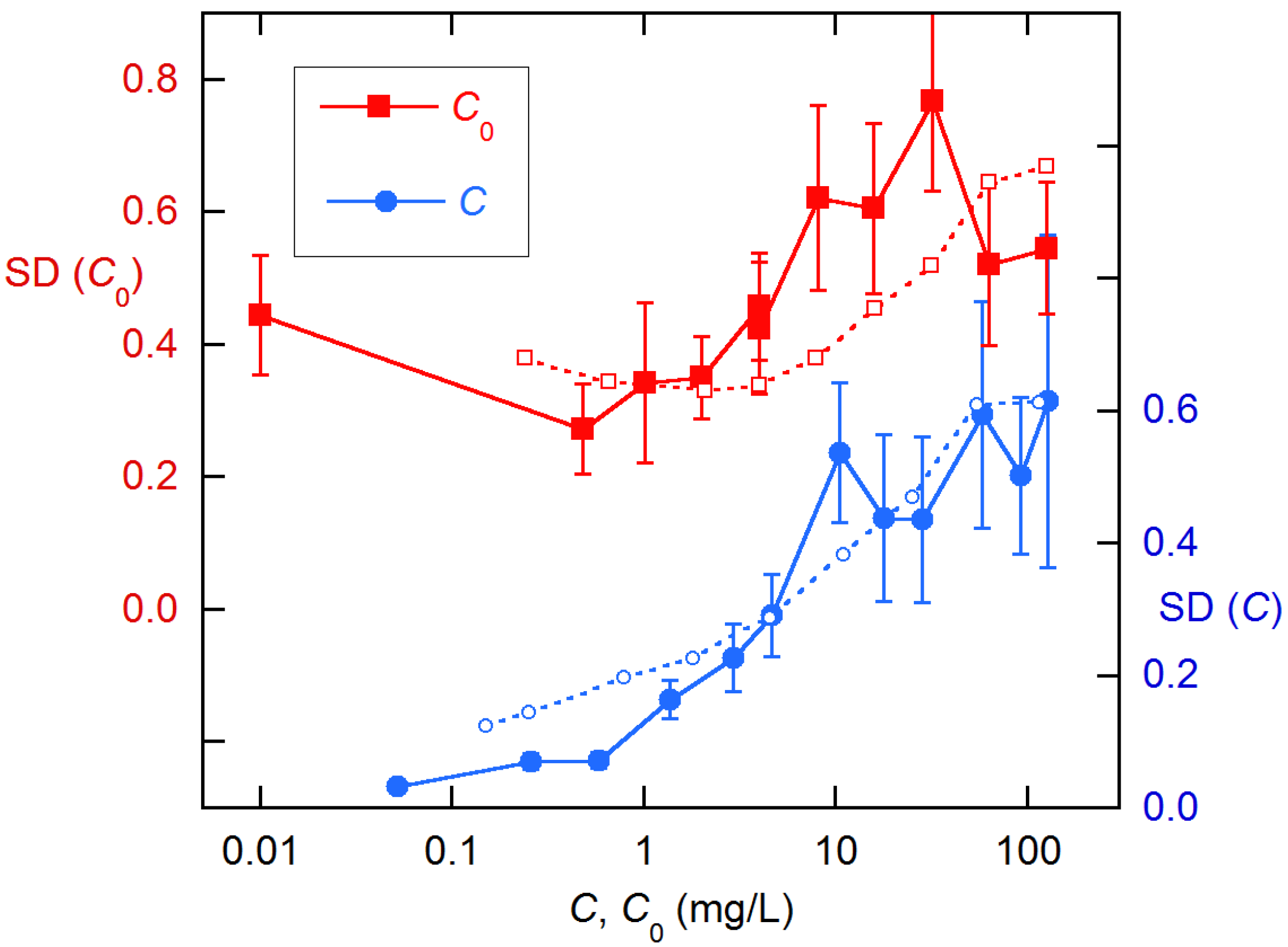
In displaying the dispersion information for the experimental data, we show the standard deviation (SD) for C₀ from the statistics for all residuals sharing a common C₀, and similarly for C (where residuals for differing C are grouped by their proximity for the statistical averaging). This means typically 10–20 residuals for each displayed value, for which the relative SD (RSD) is (2(n − 1))^−1/2, where n is the number of averaged residuals. The displayed error bars are based on these values.

Computational Methods. The global fitting, MC simulations, and residuals analysis were conducted with in-house FORTRAN codes run in Microsoft FORTRAN. For single uncertain variables, similar codes are given in refs. [16,21]. The codes for the TV method are as described in refs. [11,13,22,23]. We also used the KaleidaGraph (KG) program for simple linear and nonlinear models, both unweighted and weighted. The KG nonlinear fitting routine does not appear capable of implementing the TV method; however, it and similar analysis packages can handle multiple uncertain variables with the effective variance (EV) methods.

In the EV method used in [9] with Equation (6) as the fit model, the effective variance is

$${\sigma }_{\mathrm{eff},i}^2={\sigma }_{C_0,i}^2{\left({\displaystyle \frac{\partial f}{\partial C_0}}\right)}_i^2+{\sigma }_{C,i}^2{\left({\displaystyle \frac{\partial f}{\partial C}}\right)}_i^2$$

(10)

The weights are then taken as w_i = σ_eff,i⁻² and must be adjusted iteratively to obtain convergence, usually in ~10 cycles. A variation of this method gives near-TV results for nonlinear models and identical results for straight-line models. This EV₂ method [13,14] is also easy to implement in KG and Excel [24]. Again, using Equation (6) as the fit model, the minimization target is the sum over all points of f(C,C₀)_i²/σ_eff,i². The dependence of the weights on the parameters [through (∂f/∂C)] is thus automatically a part of the iterative parameter adjustment process in the EV₂ method.

Our reported parameter SEs are the square roots of the diagonal elements of the covariance matrix. There are two choices here [19]: (1) If the data variances are thought to be known absolutely, the factor α after Equation (5) is taken as 1.0 to give V_prior. (2) Alternatively, the factor α = S_TV/ν is incorporated to give V_post, where ν is the number of statistical degrees of freedom, equal to the number of fitted points n minus the number of adjustable parameters p. Given the approximate nature of our estimation of the data VFs, we report post-SEs.

3. Experiments and Data

The experimental details are given elsewhere [25] and discussed briefly in the Supplementary Materials (SI). The five soils are acidic pasture soils from the higher rainfall coastal zone of Eastern Australia: Camden (KA), Flaxley (FL), Glenmore (MO), Moss Vale (MA), and Richmond (D). A table summarizing their key properties is included in the Supplementary Materials (SI), where all the data are also presented.

4. Results and Discussion

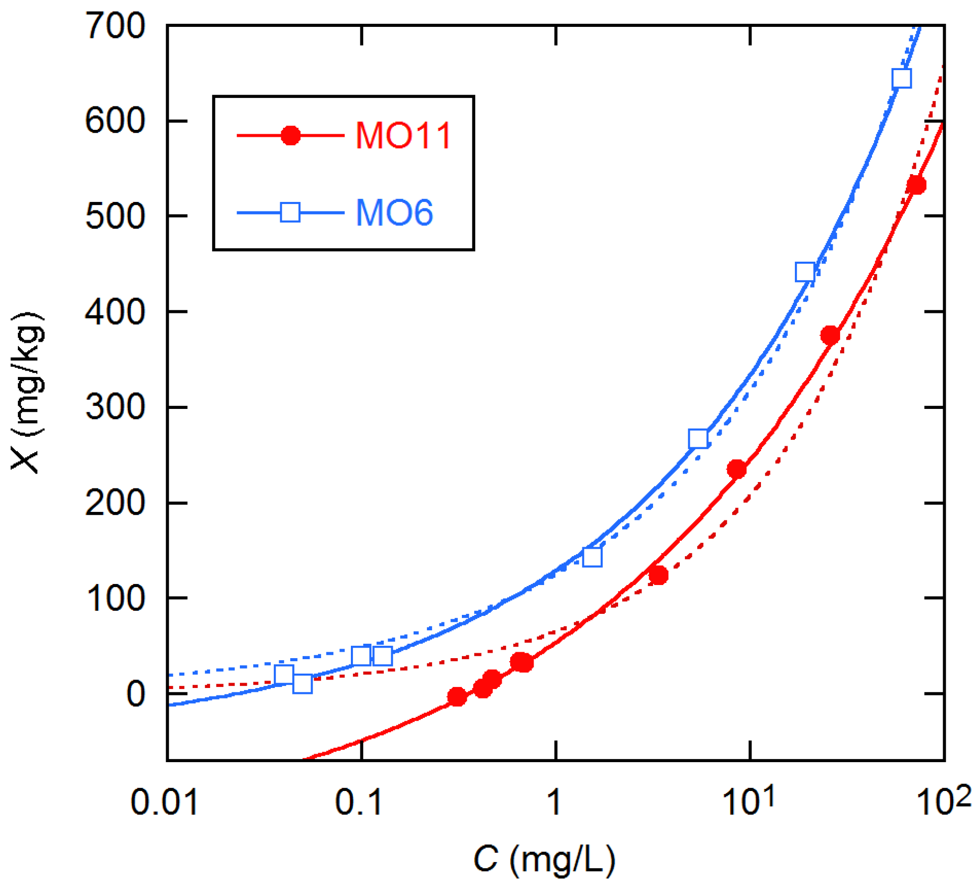
Preliminary Least-Squares Analysis. Figure 1 illustrates results from sorption experiments on MO soil having two different fertilizer pre-exposures, P_f. The need for Q in the fit model of Equation (3) is clear from the fit results with and without this term. 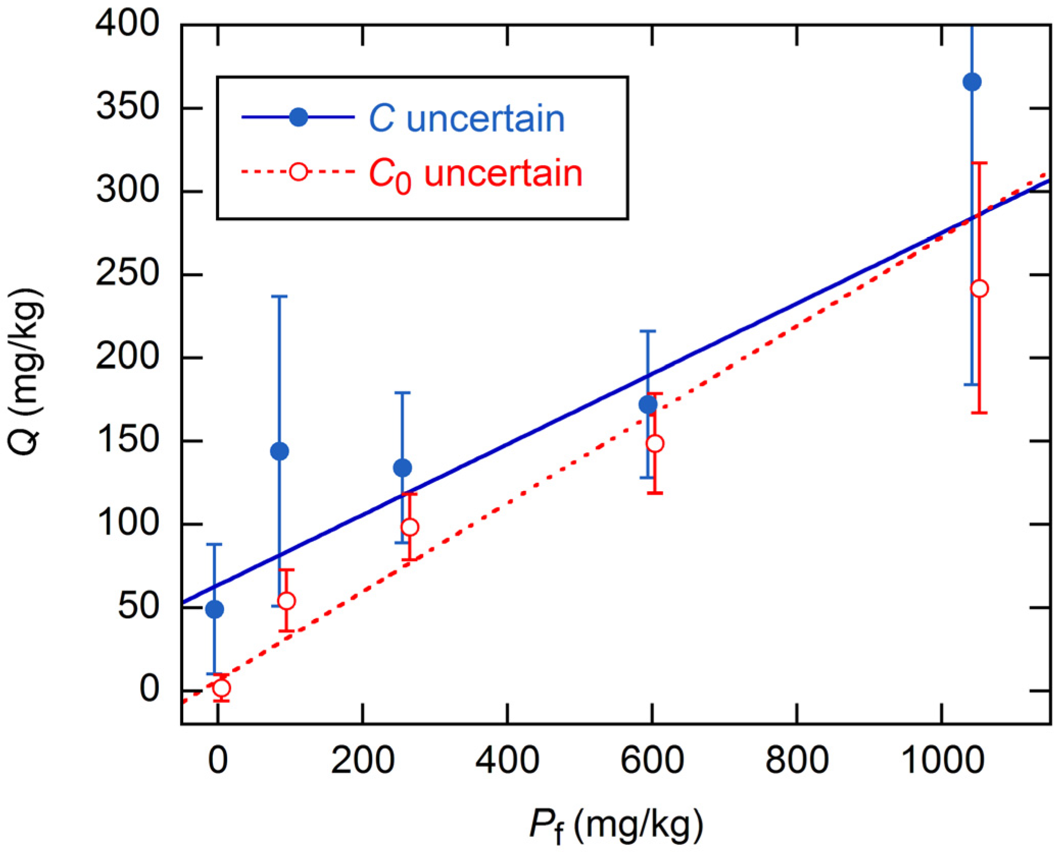As has been noted, analysis of these data using Equations (3) and (4) usually treats C as error-free and C₀ as uncertain and gives identical results for the parameters and their SEs (see Supplementary Materials (SI) for an example). On the other hand, analysis using Equations (4) and (6) with C₀ error-free and C with constant uncertainty gives consistently larger and more uncertain estimates of Q, as is shown for the KA soils in Figure 2.

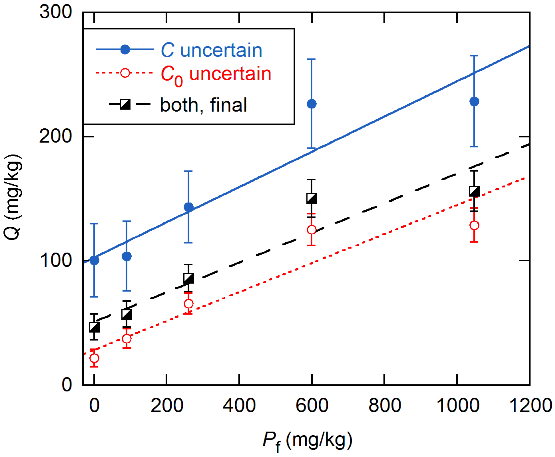
Figure 3 shows the Qs obtained for the KA soils with the global model, for the assumptions of constant error in C₀ alone and in C alone. For comparison, we include results obtained by inverse-variance weighting with the final data VFs (discussed below). For all three error models, the linearity of Q from the global fits is improved over that from individual fits, as was shown for the KA soils in Figure 2. Further, all slopes are smaller by a factor of ~2, and all intercepts are statistically significant.

To show the sensitivity of results to the choice of fitting method, we compare in

Table 1. Comparison of results obtained for the MO5 soil analyzed with three NLS methods, for constant uncertainty in C, C₀, and both.

Method
Data σ	Parameter a	EV	EV2	TV
σC = 1, σC0 = 0	a	247(47) b	254(50)	252(48)
	b	0.239(26)	0.236(27)	0.237(26)
	Q	283(54)	290(58)	288(56)
	S c	0.507	0.506	0.496
σC = 0, σC0 = 1 d	a		197(36)
	b		0.272(29)
	Q		226(40)
	S		2.95
σC = 1, σC0 = 1	a	237(46)	242(49)	241(48)
	b	0.245(28)	0.242(28)	0.243(28)
	Q	271(53)	277(56)	276(54)
	S	0.427	0.426	0.421

^a Units mg/kg for a and Q; b dimensionless. ^b Quantities in parentheses are standard errors (SE), in terms of final displayed digits, e.g., 247(47) = 247 ± 47. ^c Sum of squared residuals, using Equation (6) as fit model (R = 10 L/kg) and Equation (10) for weighting. ^d All results identical.

results obtained for one soil sample analyzed with the three different NLS methods described above. The EV₂ results are closer to TV than are the EV results, but in no case are the differences large compared with the parameter SEs. This general agreement is maintained with heteroscedastic variables, and the differences become even less significant when the uncertainties in estimating the data VFs are acknowledged. Thus, users can expect satisfactory results from all three methods.

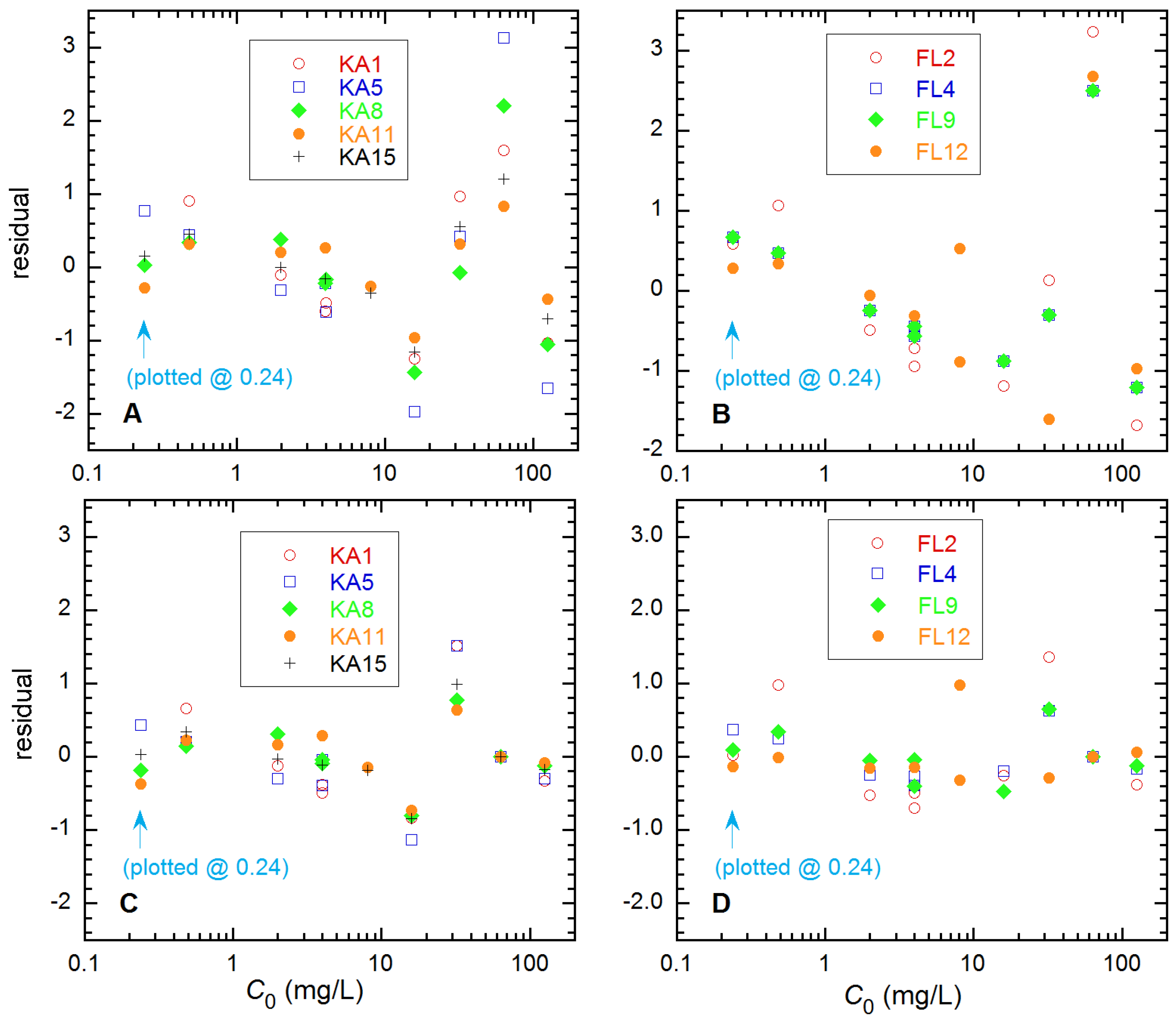
Data Variance Function Estimation. Initially, the data for each soil type and fertilizer P_f were fitted to the three-parameter model of Equation (6) assuming constant uncertainty for C₀ and zero for C, and the reverse. The residuals from all data for a given soil type were then examined for systematic effects. Three of the soil types gave no clear such effects, but two did, as shown in Figure 4, before and after removal of the largest outlier values at C₀ = 63.5 mg/L. For the FL soils, the systematic effects are negligible in frame D, but they persist for the KA soils in frame C. The behavior for FL is consistent with an erroneously prepared solution, but that for KA could as well indicate limitations in the Freundlich model for this soil. In this regard, removal of the highest concentration data (C₀ = 125.6 mg/L) improved the fit S values as much as did removal of those at C₀ = 63.5 mg/L. As is discussed below, these two choices give significantly different Q estimates for the KA soils. The residuals patterns for C-uncertain resembled those for C₀ but with reversed signs (from Equation (6)) and ~30% smaller magnitude.

Figure 5 shows the residual SDs for analysis with the global model, treating in turn C and C₀ as having constant uncertainty. (The MA soil data were much noisier, with several outliers, so they were omitted from these computations). If either of these simple error models were correct, the residual variances would be approximately constant for one of these. Both displays show a rise with increasing C and C₀, indicating heteroscedasticity, error contributions from both variables, or both effects. By comparing these results with results from MC simulations for various assumptions about the data errors, we can hope to discern the actual situation.

The MC procedures used to obtain the final estimated VFs shown in Figure 5 are discussed in the Supplementary Materials (SI). The results are

σ_C = 0.05 + 0.02 C^1/2,

(11a)

σ_C0 = 0.2 + 0.05 C₀^1/2.

(11b)

The agreement in Figure 5 is less than stellar, but it should suffice to yield high-quality results, considering that even the most extreme assumptions about the data error do not drastically alter the Qs, for example, as illustrated above in Figure 3.

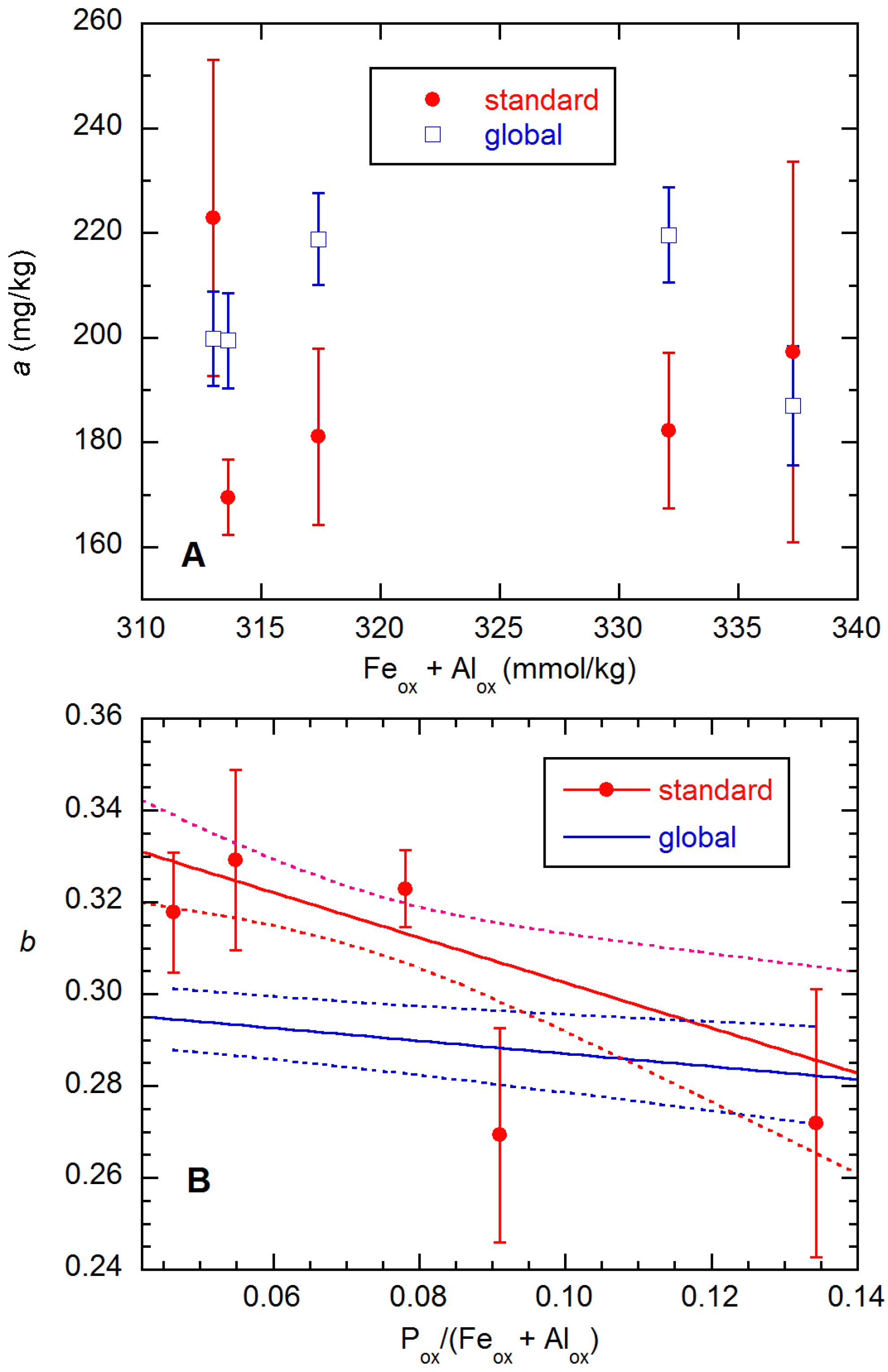
Weighted Global Analysis. In Figure 6, we compare results for the a and b parameters from standard (unweighted fits of individual datasets using Equation (3)) and global fits (with weighting based on the SD expressions in Equation (11)) of the MO soil data. Because of the pH dependence, the global a values from Equation (7a) do not fall on a straight line, while the global b values are linear in the abscissa by definition. Most of the values for the two methods disagree by more than their combined SEs, which can be taken as a measure of inconsistency.

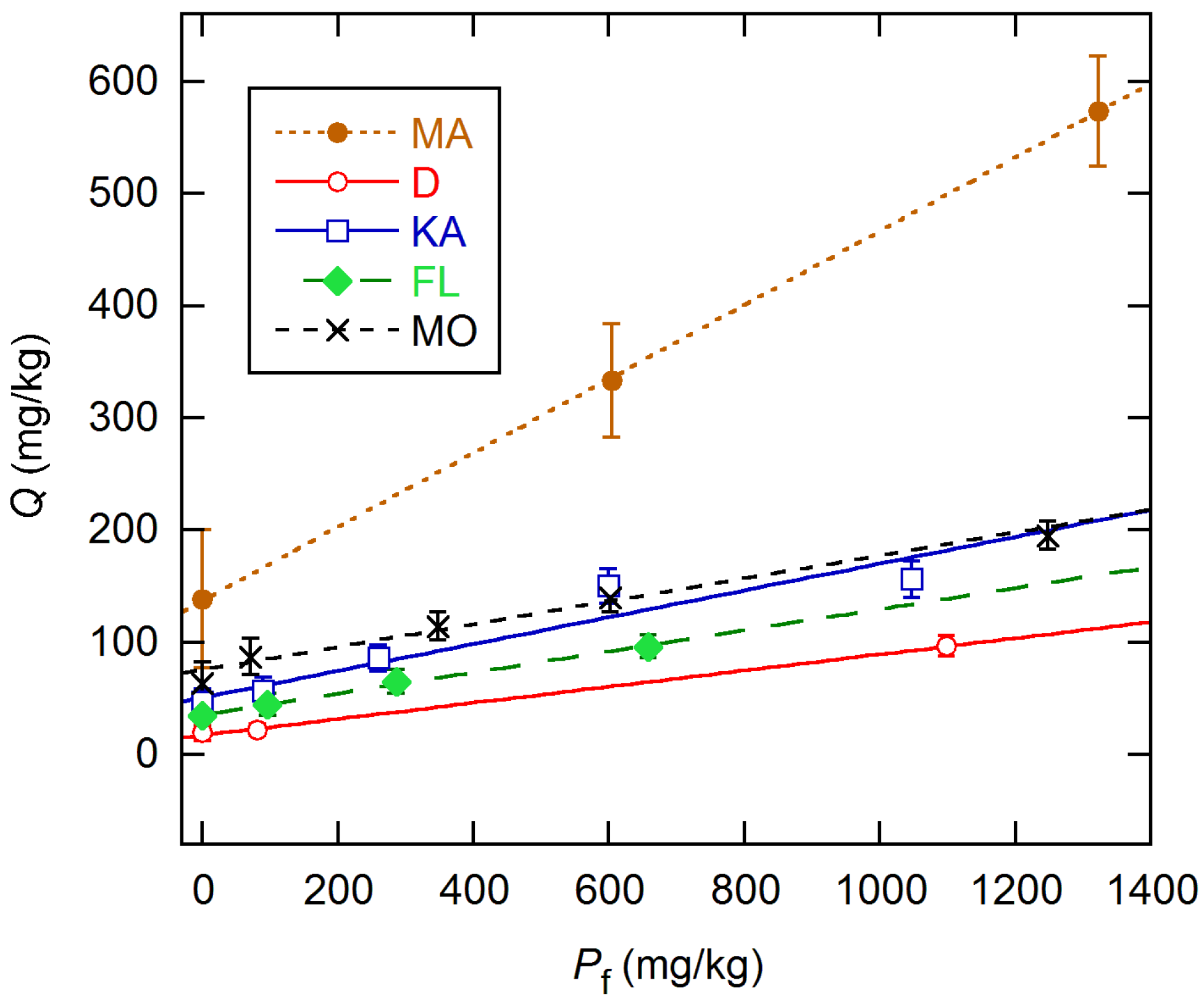
Figure 7 shows the Qs obtained analyzing all data with the weighted global model. The dependence on P_f is linear in all cases, and all intercepts are statistically significant. The slopes for the last four soils range from 0.072 to 0.119, while that for MA is three times larger.

When the global model was changed to incorporate the linear dependence of Q on P_f through Equation (8), results for four of the soils remained close to those obtained with individual Q values, as shown in Figure 7. However, for the KA soil type, the apparently modest deviations in Figure 3 and Figure 7 are much more significant than they appear, because the Q values are highly correlated through their common assessment in the global model. Accordingly, the reduced χ² (RCS = S_TV/ν) rose by a factor of 6 to 10.6. The KA results given in

Table 2. Results from global analyses of sorption data for five soil types.

Soil Type
Parameter a,b	MA c	D	KA d	FL	MO
Reduced χ2	1.58	0.35	1.61	1.02	1.40
a0	616(43)	43(4)	107(10)	91(8)	129(21)
a1		1.15(10)	0.97(26)	−0.50(7)	−0.53(19)
a2				2.1(1.4) e	7(1) e
A	380	80	140	190	320
b0	0.243(9)	0.306(18)	0.312(21)	0.336(15)	0.301(8)
b1	0.305(19)	0.320(43)	0.286(86)	0.12(10)	0.14(9)
Q1	138 (51)	20(5)	48(10)	37(7)	63(13)
[Pf, mg/kg]	[0]	[0]	[0]	[0]	[0]
Q2	333(47)	22(4)	57(10)	43(6)	88(11)
[Pf, mg/kg]	[604]	[81]	[90]	[96]	[71]
Q3	573(45)	98(7)	86(11)	65(7)	113(8)
[Pf, mg/kg]	[1322]	[1098]	[260]	[286]	[348]
Q4			149(15)	97(7)	141(8)
[Pf, mg/kg]			[599]	[658]	[602]
Q5			155(16)		195(9)
[Pf, mg/kg]			[1047]		[1248]
q0	133(49)	16(4)	40(9)	35(6)	81(9)
q1	0.331(8)	0.070(2)	0.160(12)	0.098(5)	0.108(8)

^a All parameters from the seven-parameter model incorporating Equations (7) and (8), except Qs from the alternative model using individual values in place of Equation (8). Quantities in parentheses are standard errors (SE), in terms of final displayed digits, e.g., 616(43) = 616 ± 43. SEs are post, which makes them independent of the weight scaling factor α defined after Equation (5). Omitted parameters were not statistically significant, having SEs exceeding their magnitudes. Displayed results were obtained setting these to zero and refitting. ^b All quantities in units appropriate to give sorbed amounts in mg/kg, with solution concentrations in mg/L (C, C₀) and mol/L (H⁺); units for Fe_ox, Al_ox, P_ox, and A, mmol/kg. ^c With omission of data for P_f = 0, a₀, b₀, b₁, Q₂, Q₃, respectively = 384(17), 0.356(11), 0.578(31), 121(17), and 335(17); q₀ and q₁ = −60(17) and 0.299(6), respectively. ^d Data for P_f = 1047 mg/L omitted from analysis. ^e Reference pH value in Equation (7a), B = 6.

were obtained by deleting the data for the fifth concentration. Results for other data selections are discussed in the Supplementary Materials (SI). As can be seen from Table 2, the pH parameter a₂ was statistically significant for only the MO and FL soils. The other parameters were significant except for one case for a₁ (MA). The RCS values vary somewhat more than the expected ~1.0(3) for equivalent data for all soils, but they are not drastically in conflict with this, which was an assumption in the estimation of the VFs.

The much stronger dependence of Q on P_f for the MA soils prompted us to examine the MA fits more closely. We found that the results for both global models were unduly sensitive to the deletion of high-C₀ points for the MA1 samples (P_f = 0). These results are discussed in more detail in the Supplementary Materials (SI), and we include the results obtained deleting all MA1 data in a footnote in Table 2.

Similarly, the great sensitivity of the KA results to the choice of included data means that those results must be considered more uncertain than is indicated by the KA parameter SEs in Table 2. This behavior heightens concern that the Freundlich model may not be suitable for the KA soils. The problem is discussed in more detail in the Supplementary Materials (SI), which also includes all the data, tabulated results for the individual-Q global model, and results from several alternative global fits of the KA data. All these results assume error-free oxalate assays and pHs, when in fact these are all measured quantities subject to uncertainty. Allowing for their uncertainty is not simple, as single measurements of each of these apply to all the data for a given P_f. Spot checks of ±4% changes in P_ox and (Fe_ox + Al_ox) in selected datasets gave smaller % changes in q₀ and q₁, so such effects are likely much smaller than the SEs reported in Table 2.

5. Conclusions

Although we have found possible use of global fitting methods in analysis of the time dependence of sorption (methods not described) [26,27], we believe the present work is the first such analysis of the dependence on fertilizer treatment. In this, we have also addressed common shortfalls—the tacit treatment of the measured C values as error-free and the failure to weight the data in accord with their often strong heteroscedasticity. We have allowed for uncertainty in both C and C₀, the latter considered as a stand-in for experimental procedures other than direct measurement, like the preparation of soil/solution mixtures. To estimate the variances in C and C₀, we have used residuals analysis incorporating a novel Monte Carlo trial-and-error procedure.

It is worth emphasizing that the most important result of the VF estimation efforts was the need to include some uncertainty in C. This need can be understood from the observation that most of the sorption experiments included some experiments where, within uncertainty, the measured C was 0.00 (see Supplementary Materials (SI)) [28,29]. To avoid computational problems, such values were typically set to a very small value, like C = 0.0001 mg/L, which is reasonable, since simplest residuals analysis indicated σ_C ~ 0.1 mg/L. (Note that σ_C is numerically ~500 times the absorbance uncertainty, from the conversion of the spectrophotometric absorbance to C). Taking typical a and b values of 100 mg/kg and 0.3, respectively, the values of aC^b range from 50 down to 6 mg/kg as C drops from 0.1 to 0.0001 mg/L. The differences in these values hugely exceed any reasonable uncertainty for X and C₀—roughly 0.3 mg/L for the latter from simplest residuals analysis. Allowing for even a small uncertainty in C completely neutralizes such problems. Anyone analyzing sorption data without allowing for uncertainty in C, as is customary in the use of Equation (3) as the fit model, should take care to ensure that these low-C problems do not affect the analysis.

The practical motivation for phosphate sorption studies of the type treated here is optimizing the balance between the needs for plant nutrition and the environment. The global analysis of data from multiple fertilizer pretreatments provides greatly improved estimates of the parameters in the Freundlich model, of which Q, the pre-existing P, is mainly of interest in this regard. The linear increase in Q with P_f implies that the increase is attributable to the fertilizer, hence represents bioavailable P. However, since Q is just a parameter in an empirical model, we cannot be sure that it is quantitatively reliable. Further, the finite Q₀ values for P_f = 0 represent P of unknown origin. These are among several questions about precisely what is measured in P sorption studies and various assays, answers to which are needed for a complete and reliable assessment of the crops-vs.-environment phosphate balance [25].