
Can Low-Cost, Handheld Spectroscopy Tools Coupled with Remote Sensing Accurately Estimate Soil Organic Carbon in Semi-Arid Grazing Lands?

 , ,
, ,  ,
,
Abstract
:1. Introduction
2. Materials and Methods
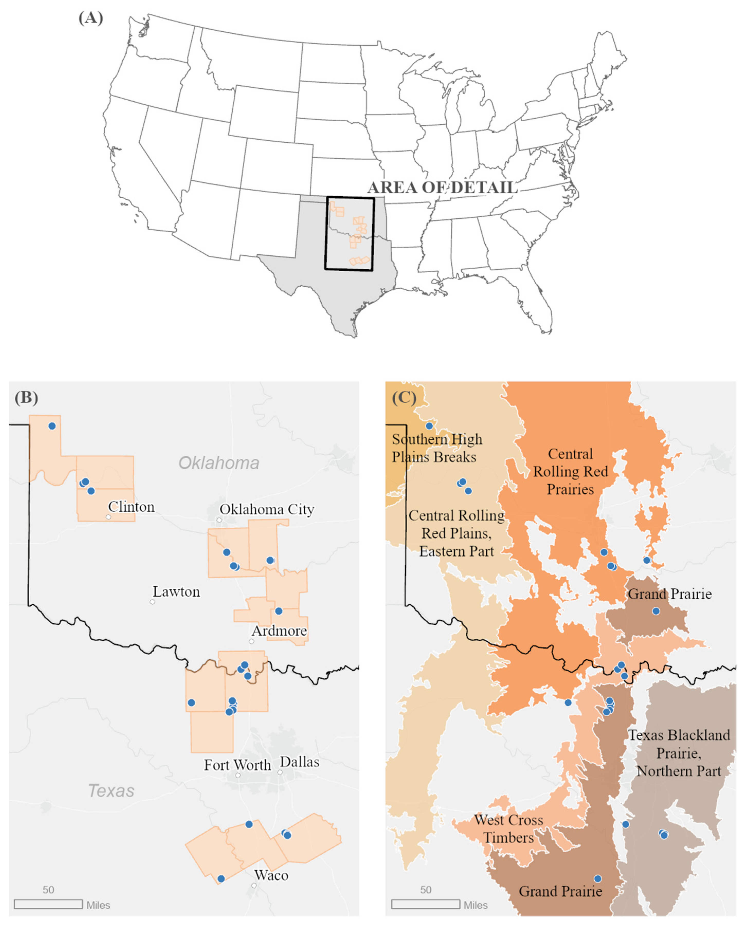
2.1. Study Sites
2.2. Sampling Design
2.3. Soil Sampling
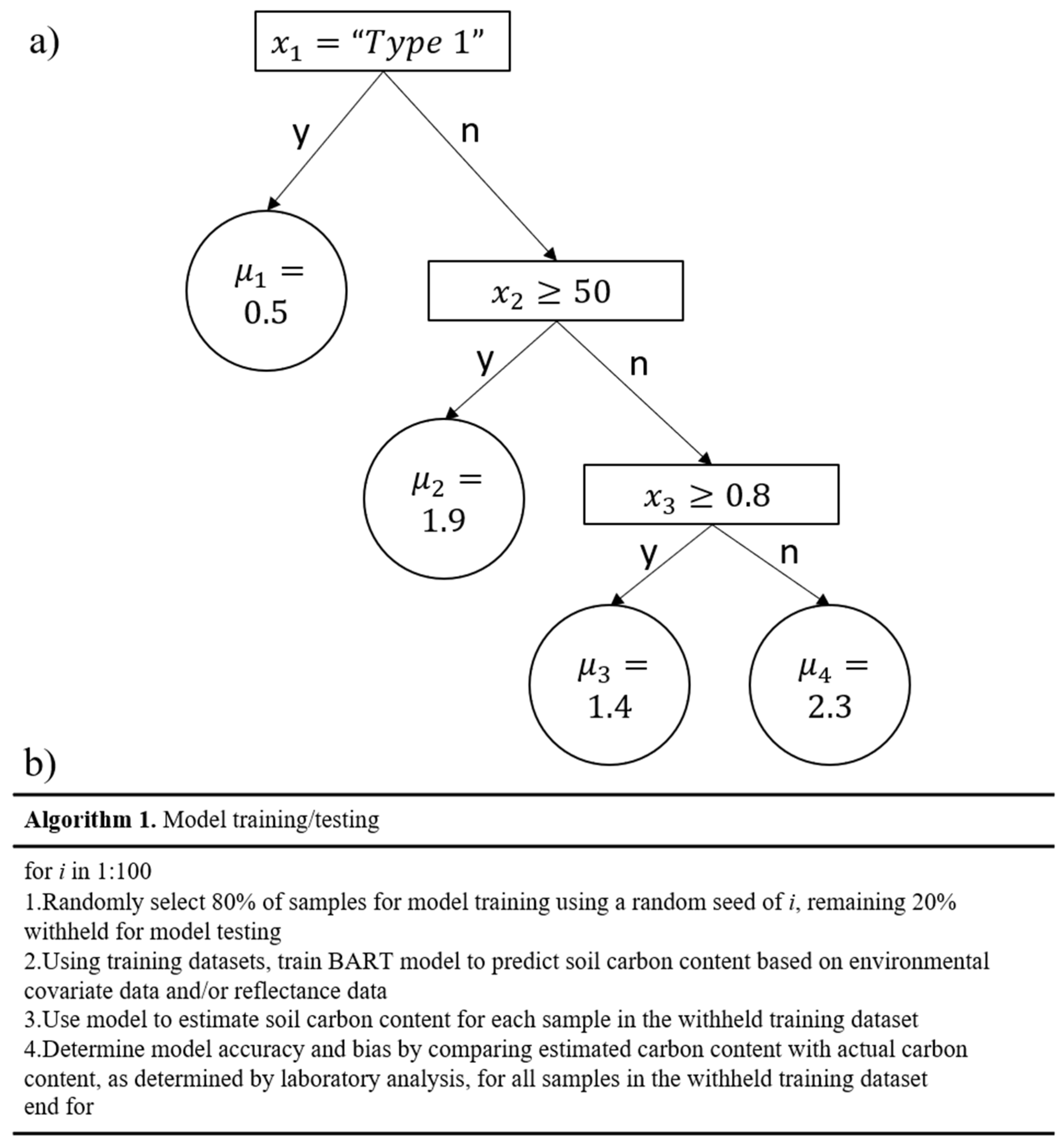
2.4. Statistical Analysis
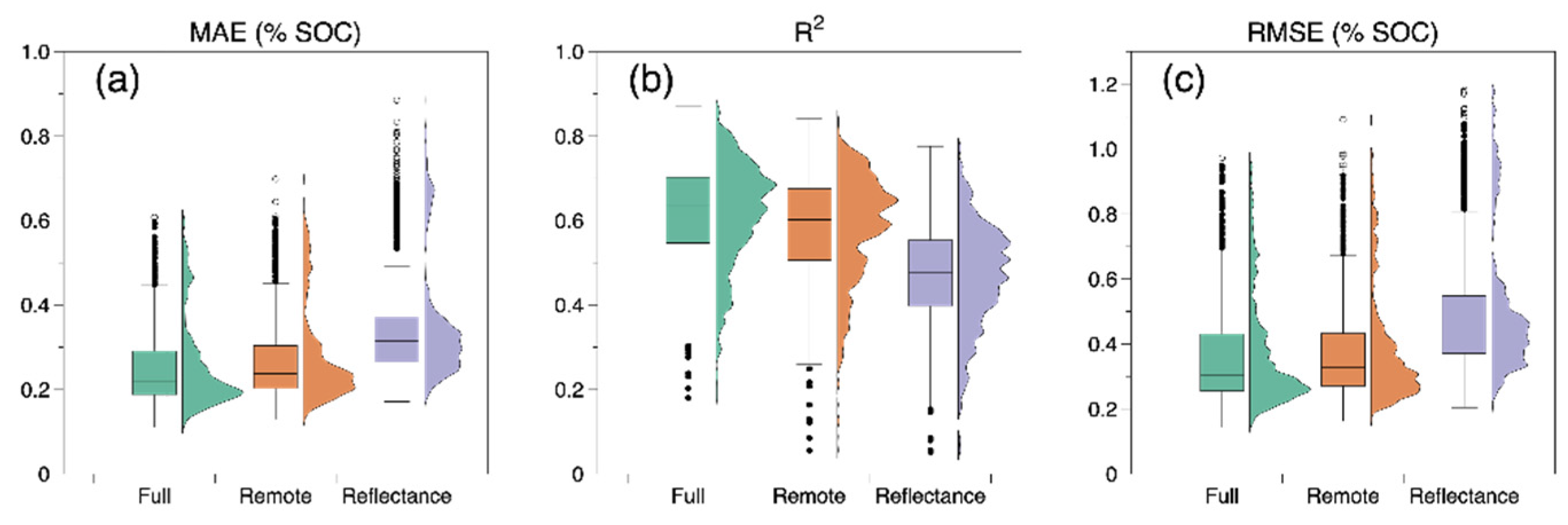
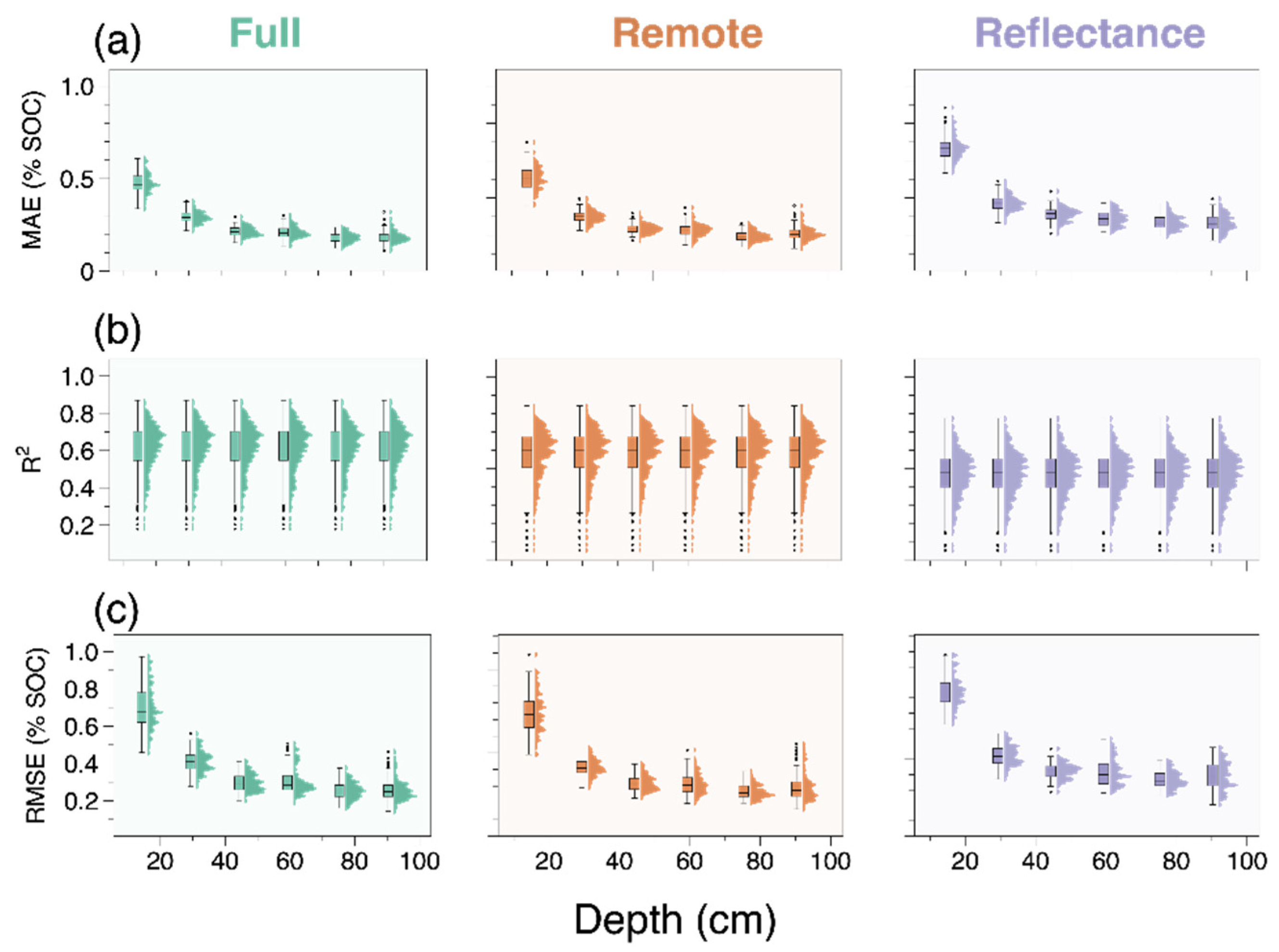
3. Results
4. Discussion
5. Conclusions
Author Contributions
Funding
Institutional Review Board Statement
Informed Consent Statement
Data Availability Statement
Acknowledgments
Conflicts of Interest
References
- Rumpel, C.; Amiraslani, F.; Koutika, L.S.; Smith, P.; Whitehead, D.; Wollenberg, E. Put more carbon in soils to meet Paris climate pledges. Nature 2018, 564, 32–34. [Google Scholar] [CrossRef] [PubMed] [Green Version]
- Lal, R. Soil carbon sequestration to mitigate climate change. Geoderma 2004, 123, 1–22. [Google Scholar] [CrossRef]
- Chabbi, A.; Lehmann, J.; Ciais, P.; Loescher, H.W.; Cotrufo, M.F.; Don, A.; SanClements, M.; Schipper, L.; Six, J.; Smith, P.; et al. Aligning agriculture and climate policy. Nat. Clim. Chang. 2017, 7, 307–309. [Google Scholar] [CrossRef]
- Lal, R. Global potential of soil carbon sequestration to mitigate the greenhouse effect. Crit. Rev. Plant Sci. 2003, 22, 151–184. [Google Scholar] [CrossRef]
- Eglin, T.; Ciais, P.; Piao, S.; Barre, P.; Bellassen, V.; Cadule, P.; Chenu, C.; Gasser, T.; Koven, C.; Reichstein, M.; et al. Historical and future perspectives of global soil carbon response to climate and land-use changes. Tellus B Chem. Phys. Meteorol. 2010, 62, 700–718. [Google Scholar] [CrossRef] [Green Version]
- Paustian, K.; Lehmann, J.; Ogle, S.; Reay, D.; Robertson, G.P.; Smith, P. Climate-smart soils. Nature 2016, 532, 49–57. [Google Scholar] [CrossRef] [PubMed] [Green Version]
- Lal, R. Soil carbon sequestration impacts on global climate change and food security. Science 2004, 304, 1623–1627. [Google Scholar] [CrossRef] [PubMed] [Green Version]
- Williams, A.; Hunter, M.; Kammerer, M.; Kane, D.A.; Jordan, N.R.; Mortensen, D.A.; Smith, R.G.; Snapp, S.; Davis, A.S. Soil Water Holding Capacity Mitigates Downside Risk and Volatility in US Rainfed Maize: Time to Invest in Soil Organic Matter? PLoS ONE 2016, 11, e0160974. [Google Scholar] [CrossRef]
- Lal, R. Sequestering carbon and increasing productivity by conservation agriculture. J. Soil Water Conserv. 2015, 70, 55A–62A. [Google Scholar] [CrossRef] [Green Version]
- Pozdnyakova, L.; Giménez, D.; Oudemans, P.V. Spatial Analysis of Cranberry Yield at Three Scales. Agron. J. 2005, 97, 49–57. [Google Scholar] [CrossRef]
- Bellon-Maurel, V.; McBratney, A. Near-infrared (NIR) and mid-infrared (MIR) spectroscopic techniques for assessing the amount of carbon stock in soils—Critical review and research perspectives. Soil Biol. Biochem. 2011, 43, 1398–1410. [Google Scholar] [CrossRef]
- Gomez, C.; Rossel, R.V.; McBratney, A. Soil organic carbon prediction by hyperspectral remote sensing and field vis-NIR spectroscopy: An Australian case study. Geoderma 2008, 146, 403–411. [Google Scholar] [CrossRef]
- Wetzel, D.L. Near-infrared reflectance analysis. Anal. Chem. 1983, 55, 1165A–1176A. [Google Scholar] [CrossRef]
- Cozzolino, D.; Morón, A. The potential of near-infrared reflectance spectroscopy to analyse soil chemical and physical characteristics. J. Agric. Sci. 2003, 140, 65–71. [Google Scholar] [CrossRef]
- Cozzolino, D.; Morón, A. Potential of near-infrared reflectance spectroscopy and chemometrics to predict soil organic carbon fractions. Soil Tillage Res. 2006, 85, 78–85. [Google Scholar] [CrossRef]
- Dalal, R.C.; Henry, R.J. Simultaneous Determination of Moisture, Organic Carbon, and Total Nitrogen by Near Infrared Reflectance Spectrophotometry. Soil Sci. Soc. Am. J. 1986, 50, 120–123. [Google Scholar] [CrossRef]
- Morra, M.J.; Hall, M.H.; Freeborn, L.L. Carbon and Nitrogen Analysis of Soil Fractions Using Near-Infrared Reflectance Spectroscopy. Soil Sci. Soc. Am. J. 1991, 55, 288–291. [Google Scholar] [CrossRef]
- Reeves, J.; McCarty, G.; Mimmo, T. The potential of diffuse reflectance spectroscopy for the determination of carbon inventories in soils. Environ. Pollut. 2002, 116, S277–S284. [Google Scholar] [CrossRef]
- Volkan Bilgili, A.; van Es, H.M.; Akbas, F.; Durak, A.; Hively, W.D. Visible-near infrared reflectance spectroscopy for assessment of soil properties in a semi-arid area of Turkey. J. Arid Environ. 2010, 74, 229–238. [Google Scholar] [CrossRef]
- Gao, Y.; Cui, L.; Lei, B.; Zhai, Y.; Shi, T.; Wang, J.; Chen, Y.; He, H.; Wu, G. Estimating Soil Organic Carbon Content with Visible–Near-Infrared (Vis-NIR) Spectroscopy. Appl. Spectrosc. 2014, 68, 712–722. [Google Scholar] [CrossRef]
- Van Groenigen, J.W.; Mutters, C.; Horwath, W.; Van Kessel, C. NIR and DRIFT-MIR spectrometry of soils for predicting soil and crop parameters in a flooded field. Plant Soil 2003, 250, 155–165. [Google Scholar] [CrossRef]
- Reeves, J. Near- versus mid-infrared diffuse reflectance spectroscopy for soil analysis emphasizing carbon and laboratory versus on-site analysis: Where are we and what needs to be done? Geoderma 2010, 158, 3–14. [Google Scholar] [CrossRef]
- Kusumo, B.H.; Hedley, M.J.; Hedley, C.B.; Tuohy, M.P. Measuring carbon dynamics in field soils using soil spectral reflectance: Prediction of maize root density, soil organic carbon and nitrogen content. Plant Soil 2010, 338, 233–245. [Google Scholar] [CrossRef]
- Minasny, B.; Tranter, G.; McBratney, A.B.; Brough, D.M.; Murphy, B.W. Regional transferability of mid-infrared diffuse reflectance spectroscopic prediction for soil chemical properties. Geoderma 2009, 153, 155–162. [Google Scholar] [CrossRef]
- Brown, D.J.; Shepherd, K.D.; Walsh, M.G.; Dewayne Mays, M.; Reinsch, T.G. Global soil characterization with VNIR diffuse reflectance spectroscopy. Geoderma 2006, 132, 273–290. [Google Scholar] [CrossRef]
- Muñoz, J.D.; Kravchenko, A. Soil carbon mapping using on-the-go near infrared spectroscopy, topography and aerial photographs. Geoderma 2011, 166, 102–110. [Google Scholar] [CrossRef]
- Peng, Y.; Xiong, X.; Adhikari, K.; Knadel, M.; Grunwald, S.; Greve, M.H. Modeling Soil Organic Carbon at Regional Scale by Combining Multi-Spectral Images with Laboratory Spectra. PLoS ONE 2015, 10, e0142295. [Google Scholar] [CrossRef] [Green Version]
- Soil Survey Staff. Natural Resources Conservation Service, United States Department of Agriculture. Web Soil Survey. Available online: https://websoilsurvey.nrcs.usda.gov (accessed on 10 March 2022).
- Bettigole, C.; Szeto, S.; Covey, K.; Wood, S.; Kane, D.; Chandler, M.; Hersh, E. Stratifi 3.1. Available online: https://charliebettigole.users.earthengine.app/view/stratifi-beta-v21 (accessed on 10 March 2022).
- Pelleg, D.; Moore, A.W. X-means: Extending k-means with efficient estimation of the number of clusters. In Proceedings of the Seventeenth International Conference on Machine Learning, San Francisco, CA, USA, 29 June–2 July 2000; pp. 727–734. [Google Scholar]
- Nelson, D.W.; Sommers, L.E. Total Carbon, Organic Carbon, and Organic Matter. In Methods of Soil Analysis; Sparks, D.L., Ed.; Agronomy Monographs; SSSA Book Series; American Society of Agronomy: Madison, WI, USA, 1996; pp. 961–1010. [Google Scholar]
- Soil Survey Staff, Natural Resources Conservation Service, United States Department of Agriculture. Soil Survey Geographic (SSURGO) Database for [Survey Area, Oklahoma and Texas]. Available online: https://www.nrcs.usda.gov/wps/portal/nrcs/detail/soils/survey/?cid=nrcs142p2_053627 (accessed on 3 January 2022).
- Python API. ee Package. Available online: https://gee-python-api.readthedocs.io/en/latest/ee.html (accessed on 3 January 2022).
- Chipman, H.A.; George, E.I.; McCulloch, R.E. BART: Bayesian additive regression trees. Ann. Appl. Stat. 2010, 4, 266–298. [Google Scholar] [CrossRef]
- Kapelner, A.; Bleich, J. bartMachine: Machine Learning with Bayesian Additive Regression Trees. J. Stat. Softw. 2016, 70, 1–40. [Google Scholar] [CrossRef] [Green Version]
- Stenberg, B. Effects of soil sample pretreatments and standardised rewetting as interacted with sand classes on Vis-NIR predictions of clay and soil organic carbon. Geoderma 2010, 158, 15–22. [Google Scholar] [CrossRef] [Green Version]
- Stenberg, B.; Viscarra Rossel, R.A.; Mouazen, A.M.; Wetterlind, J. Visible and Near Infrared Spectroscopy in Soil Science. In Advances in Agronomy; Sparks, D.L., Ed.; Academic Press: Cambridge, MA, USA, 2010; pp. 163–215. [Google Scholar]
- Olatunde, K.A. Estimation of soil organic carbon using chemometrics: A comparison between mid-infrared and visible near infrared diffuse reflectance spectroscopy. West Afr. J. Appl. Ecol. 2021, 29, 1–11. [Google Scholar]
- Summers, D.; Lewis, M.; Ostendorf, B.; Chittleborough, D. Visible near-infrared reflectance spectroscopy as a predictive indicator of soil properties. Ecol. Indic. 2011, 11, 123–131. [Google Scholar] [CrossRef]
- McBride, M.B. Estimating soil chemical properties by diffuse reflectance spectroscopy: Promise versus reality. Eur. J. Soil Sci. 2021, 73, e13192. [Google Scholar] [CrossRef]
- Reyna, L.; Dube, F.; Barrera, J.A.; Zagal, E. Potential Model Overfitting in Predicting Soil Carbon Content by Visible and Near-Infrared Spectroscopy. Appl. Sci. 2017, 7, 708. [Google Scholar] [CrossRef] [Green Version]
- Jobbágy, E.G.; Jackson, R.B. The vertical distribution of soil organic carbon and its relation to climate and vegetation. Ecol. Appl. 2000, 10, 423–436. [Google Scholar] [CrossRef]
- Liski, J.; Westman, C.J. Density of organic carbon in soil at coniferous forest sites in southern Finland. Biogeochemistry 1995, 29, 183–197. [Google Scholar] [CrossRef]
- Rasse, D.P.; Rumpel, C.; Dignac, M.-F. Is soil carbon mostly root carbon? Mechanisms for a specific stabilisation. Plant Soil 2005, 269, 341–356. [Google Scholar] [CrossRef]
- Richter, D.D.; Markewitz, D. How Deep Is Soil? BioScience 1995, 45, 600–609. [Google Scholar] [CrossRef]
- Rumpel, C.; Kögel-Knabner, I. Deep soil organic matter—A key but poorly understood component of terrestrial C cycle. Plant Soil 2011, 338, 143–158. [Google Scholar] [CrossRef]
- Swift, R.S. Sequestration of carbon by soil. Soil Sci. 2001, 166, 858–871. [Google Scholar] [CrossRef]
- Gholizadeh, A.; Rossel, R.A.V.; Saberioon, M.; Borůvka, L.; Kratina, J.; Pavlů, L. National-scale spectroscopic assessment of soil organic carbon in forests of the Czech Republic. Geoderma 2020, 385, 114832. [Google Scholar] [CrossRef]
- Chen, Y.; Li, Y.; Wang, X.; Wang, J.; Gong, X.; Niu, Y.; Liu, J. Estimating soil organic carbon density in Northern China’s agro-pastoral ecotone using vis-NIR spectroscopy. J. Soils Sediments 2020, 20, 3698–3711. [Google Scholar] [CrossRef]
- Allo, M.; Todoroff, P.; Jameux, M.; Stern, M.; Paulin, L.; Albrecht, A. Prediction of tropical volcanic soil organic carbon stocks by visible-near- and mid-infrared spectroscopy. CATENA 2020, 189, 104452. [Google Scholar] [CrossRef]
- Ewing, P.M.; TerAvest, D.; Tu, X.; Snapp, S.S. Accessible, affordable, fine-scale estimates of soil carbon for sustainable management in sub-Saharan Africa. Soil Sci. Soc. Am. J. 2021, 85, 1814–1826. [Google Scholar] [CrossRef]
- Disla, J.S.; Janik, L.J.; Rossel, R.V.; Macdonald, L.; McLaughlin, M.J. The Performance of Visible, Near-, and Mid-Infrared Reflectance Spectroscopy for Prediction of Soil Physical, Chemical, and Biological Properties. Appl. Spectrosc. Rev. 2013, 49, 139–186. [Google Scholar] [CrossRef]
- Riedel, F.; Denk, M.; Müller, I.; Barth, N.; Gläßer, C. Prediction of soil parameters using the spectral range between 350 and 15,000 nm: A case study based on the Permanent Soil Monitoring Program in Saxony, Germany. Geoderma 2018, 315, 188–198. [Google Scholar] [CrossRef]
- Paul, S.; Coops, N.; Johnson, M.; Krzic, M.; Smukler, S. Evaluating sampling efforts of standard laboratory analysis and mid-infrared spectroscopy for cost effective digital soil mapping at field scale. Geoderma 2019, 356, 113925. [Google Scholar] [CrossRef]
- Chakraborty, S.; Li, B.; Weindorf, D.C.; Morgan, C.L. External parameter orthogonalisation of Eastern European VisNIR-DRS soil spectra. Geoderma 2018, 337, 65–75. [Google Scholar] [CrossRef]
- Cozzolino, D. Near infrared spectroscopy as a tool to monitor contaminants in soil, sediments and water—State of the art, advantages and pitfalls. Trends Environ. Anal. Chem. 2016, 9, 1–7. [Google Scholar] [CrossRef]
- Goff, K.; Schaetzl, R.J.; Chakraborty, S.; Weindorf, D.C.; Kasmerchak, C.; Bettis, E.A. Impact of sample preparation methods for characterizing the geochemistry of soils and sediments by portable X-ray fluorescence. Soil Sci. Soc. Am. J. 2019, 84, 131–143. [Google Scholar] [CrossRef]
- Mallet, A.; Charnier, C.; Latrille, É.; Bendoula, R.; Steyer, J.-P.; Roger, J.-M. Unveiling non-linear water effects in near infrared spectroscopy: A study on organic wastes during drying using chemometrics. Waste Manag. 2021, 122, 36–48. [Google Scholar] [CrossRef] [PubMed]
- Williams, P. Influence of Water on Prediction of Composition and Quality Factors: The Aquaphotomics of Low Moisture Agricultural Materials. J. Near Infrared Spectrosc. 2009, 17, 315–328. [Google Scholar] [CrossRef]
- Cao, Y.; Bao, N.; Liu, S.; Zhao, W.; Li, S. Reducing moisture effects on soil organic carbon content prediction in visible and near-infrared spectra with an external parameter othogonalization algorithm. Can. J. Soil Sci. 2020, 100, 253–262. [Google Scholar] [CrossRef]
- Guerrero, C.; Wetterlind, J.; Stenberg, B.; Mouazen, A.M.; Gabarrón-Galeote, M.A.; Ruiz-Sinoga, J.D.; Zornoza, R.; Rossel, R.V. Do we really need large spectral libraries for local scale SOC assessment with NIR spectroscopy? Soil Tillage Res. 2016, 155, 501–509. [Google Scholar] [CrossRef]
- Stevens, A.; Nocita, M.; Toth, G.; Montanarella, L.; van Wesemael, B. Prediction of Soil Organic Carbon at the European Scale by Visible and Near InfraRed Reflectance Spectroscopy. PLoS ONE 2013, 8, e66409. [Google Scholar] [CrossRef]


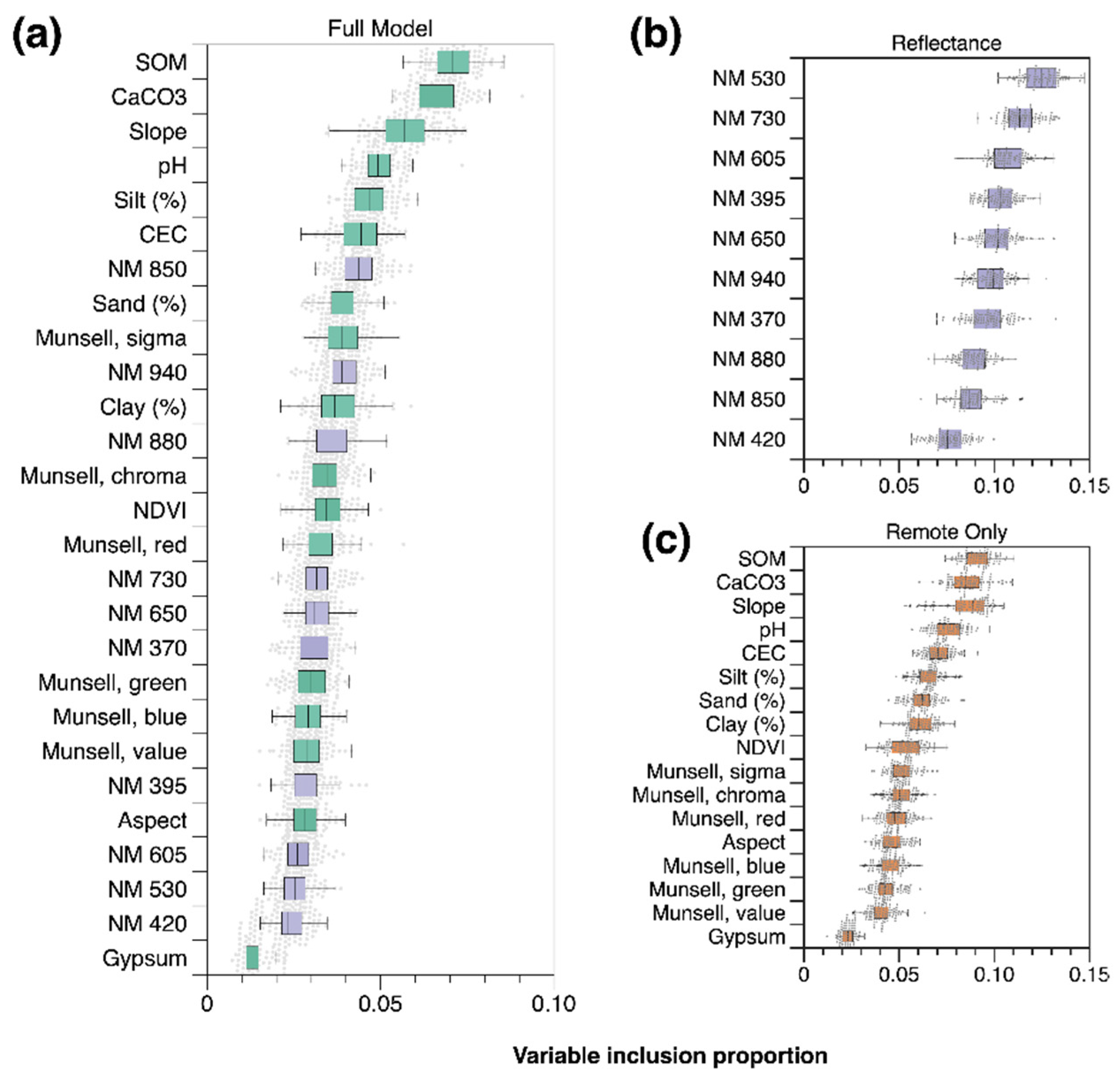
| Dataset | Category | Property |
|---|---|---|
| USDA SSURGO | Soil chemical properties | Organic matter (%) |
| Gypsum | ||
| CaCO3 | ||
| pH | ||
| Cation exchange capacity | ||
| Soil texture | Silt (%) | |
| Clay (%) | ||
| Sand (%) | ||
| Soil color | Munsell value | |
| Munsell chroma | ||
| Munsell sigma | ||
| Munsell red | ||
| Munsell green | ||
| Munsell blue | ||
| Sentinel-2 | Plant properties | Normalized differential vegetation index (NDVI) |
| USGS National Elevation Dataset | Topography | Slope |
| Aspect |
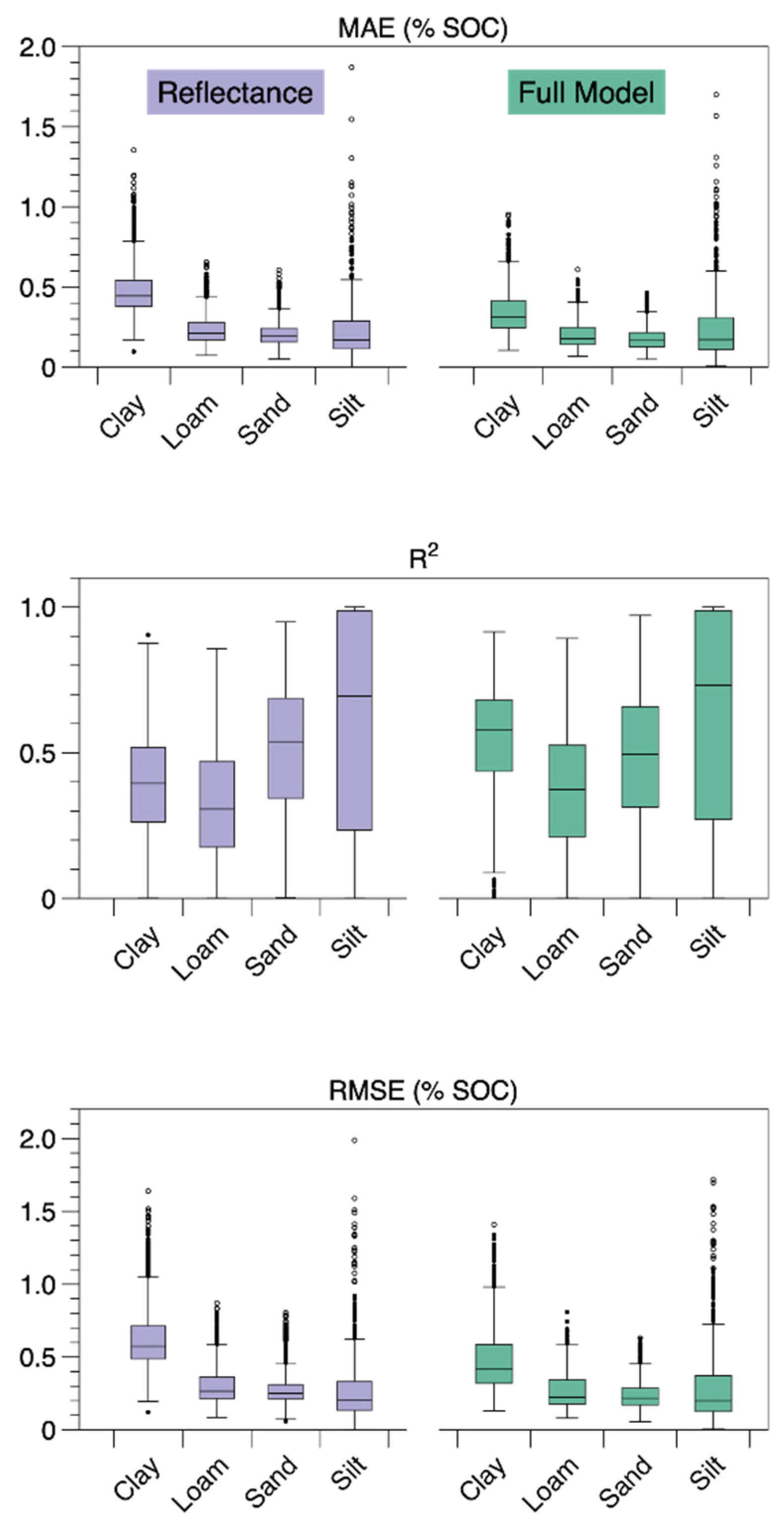
| Model Type | MAE | R2 | RMSE |
|---|---|---|---|
| Reflectance | 0.305 (0.018) | 0.54 (0.045) | 0.602 (0.041) |
| Remote | 0.303 (0.016) | 0.71 (0.051) | 0.469 (0.044) |
| Full | 0.284 (0.015) | 0.75 (0.054) | 0.447 (0.045) |
| Model Type | Reflectance | Remote | Full |
|---|---|---|---|
| Reflectance | - | 38.033 (<0.001) | 47.204 (<0.001) |
| Remote | - | - | 8.507 (<0.001) |
| Full | - | - | - |
Publisher’s Note: MDPI stays neutral with regard to jurisdictional claims in published maps and institutional affiliations. |
© 2022 by the authors. Licensee MDPI, Basel, Switzerland. This article is an open access article distributed under the terms and conditions of the Creative Commons Attribution (CC BY) license (https://creativecommons.org/licenses/by/4.0/).
Share and Cite
Goodwin, D.J.; Kane, D.A.; Dhakal, K.; Covey, K.R.; Bettigole, C.; Hanle, J.; Ortega-S., J.A.; Perotto-Baldivieso, H.L.; Fox, W.E.; Tolleson, D.R. Can Low-Cost, Handheld Spectroscopy Tools Coupled with Remote Sensing Accurately Estimate Soil Organic Carbon in Semi-Arid Grazing Lands? Soil Syst. 2022, 6, 38. https://doi.org/10.3390/soilsystems6020038
Goodwin DJ, Kane DA, Dhakal K, Covey KR, Bettigole C, Hanle J, Ortega-S. JA, Perotto-Baldivieso HL, Fox WE, Tolleson DR. Can Low-Cost, Handheld Spectroscopy Tools Coupled with Remote Sensing Accurately Estimate Soil Organic Carbon in Semi-Arid Grazing Lands? Soil Systems. 2022; 6(2):38. https://doi.org/10.3390/soilsystems6020038
Chicago/Turabian StyleGoodwin, Douglas Jeffrey, Daniel A. Kane, Kundan Dhakal, Kristofer R. Covey, Charles Bettigole, Juliana Hanle, J. Alfonso Ortega-S., Humberto L. Perotto-Baldivieso, William E. Fox, and Douglas R. Tolleson. 2022. "Can Low-Cost, Handheld Spectroscopy Tools Coupled with Remote Sensing Accurately Estimate Soil Organic Carbon in Semi-Arid Grazing Lands?" Soil Systems 6, no. 2: 38. https://doi.org/10.3390/soilsystems6020038
APA StyleGoodwin, D. J., Kane, D. A., Dhakal, K., Covey, K. R., Bettigole, C., Hanle, J., Ortega-S., J. A., Perotto-Baldivieso, H. L., Fox, W. E., & Tolleson, D. R. (2022). Can Low-Cost, Handheld Spectroscopy Tools Coupled with Remote Sensing Accurately Estimate Soil Organic Carbon in Semi-Arid Grazing Lands? Soil Systems, 6(2), 38. https://doi.org/10.3390/soilsystems6020038