Article

Toxicity-Weighted Exceedance Mapping of Heavy Metals in Urban Soils Using Sequential Indicator Simulation

by
Zsolt Zoltán Fehér
1,
Tamás Magyar
1,*,
Florence Alexandra Tóth
2 and
Péter Tamás Nagy
1
1
Institute of Water and Environmental Management, Faculty of Agricultural and Food Sciences and Environmental Management, University of Debrecen, Egyetem tér 1, H-4032 Debrecen, Hungary
2
Institute of Nutrition Science, Faculty of Agricultural and Food Sciences and Environmental Management, University of Debrecen, Egyetem tér 1, H-4032 Debrecen, Hungary
*
Author to whom correspondence should be addressed.
Soil Syst. 2026, 10(8), 89; https://doi.org/10.3390/soilsystems10080089
Submission received: 5 June 2026 / Revised: 24 July 2026 / Accepted: 27 July 2026 / Published: 5 August 2026
(This article belongs to the Special Issue Use of Modern Statistical Methods in Soil Science)

Abstract

Heavy metal contamination in urban topsoil is one of the most serious environmental threats to children’s health, particularly through ingestion, dermal contact, and inhalation exposure routes. The objectives of this study were: (1) to assess the probabilistic exceedance-based priority of eight heavy metals (As, Cd, Co, Cr, Cu, Ni, Pb, and Zn) with respect to regulatory threshold exceedance in Debrecen, Hungary; (2) to map the spatial distribution of exceedance probabilities using sequential indicator simulation (SISIM) with 100 equiprobable realizations per element (1000 for Cr) on a 50 m grid; and (3) to develop a toxicologically weighted composite exceedance index based on the Hungarian regulatory action thresholds and classify the results into priority categories. For Cd, the exceedance probability exceeded p > 0.50 in approximately 98% of the study area, and for Cr, in approximately 82% of the study area (regenerated at N   =   1000 ; the Cr threshold lies near the sample median, so the p > 0.50 area is ensemble-size sensitive and was under-converged at N   =   100 ). Approximately 86% of the study area fell into the Very Low Priority class, approximately 14% into the Low Priority class, and less than 0.1% of the area exceeded the Moderate Priority threshold. Monte Carlo perturbation of the child exposure relevance factors confirmed strong spatial rank stability of H(x) (median Spearman ρ =   0.989 ), indicating that the priority pattern is robust even though areas close to the Very Low Priority/Low Priority boundary may change class. This paper contributes single-threshold exceedance-probability maps at regulatory limits and a toxicity-weighted exceedance-priority index H ( x ) —a methodological and interpretive advance over our previous concentration mapping, using the same measurements with no new sampling. By constructing the composite index is toxicity-weighted: arsenic and cadmium carry ≈88% of the child weight, so H ( x ) chiefly resolves As- and Cd-driven priority, with the remaining metals refining local class boundaries. Receptor prioritization is a screening output to guide confirmatory sampling, not a definitive risk classification.

1. Introduction

Heavy metal contamination of urban top soils is a persistent environmental problem worldwide, particularly in rapidly expanding cities such as Debrecen, owing to the persistence, bioaccumulative potential, and toxicity of these elements even at trace concentrations. The accumulation of Pb, Cd, As, Co, Cr, Cu, Ni, and Zn in urban soils is a public health concern because these elements exert adverse effects on child development, chronic organ function, and community health through multiple exposure pathways [1,2,3,4]. The spatial distribution of these metals exhibits marked heterogeneity, attributable to proximity to emission sources, soil characteristics, and land use; thus, maps based on point estimates alone cannot capture the full range of spatial variability.
Previous characterization [5] found that heavy metal concentrations in the urban soil of the Debrecen area were governed primarily by transport, industrial activity, and geological background, based on multivariate statistical and geostatistical estimation methods. A simulation-based analysis of threshold exceedance in contaminated soils is needed to determine whether the systematic underestimation of the contamination extent results from the smoothing effect of ordinary kriging, which provides a single best estimate and does not reproduce local variability [6], or from an insufficient sampling density. Goovaerts [7] demonstrated that kriging can reduce sample variance by a factor of six in contaminated soils and that the smoothing effect systematically underestimates the spatial extent of contamination and the associated misclassification costs, whereas sequential indicator simulation (SISIM) has been shown to more reliably delineate contaminated areas than kriging-based classification [8].
In practice, however, health risk assessments for urban soils often do not explicitly account for the underestimation of extreme concentrations inherent in kriging and use deterministic hazard quotient ( H Q ) and carcinogenic risk ( C R ) calculations for kriged concentration surfaces [9,10]. Machine learning methods are increasingly used in digital soil mapping [11,12,13,14], but their reliance on variance minimization and the multi-Gaussian condition of hybrid ML-geostatistical approaches, such as regression kriging or XGBoost-SGS, can limit their suitability for regulatory exceedance problems, where the distribution tails carry the decision risk [15,16]. Few studies have examined the threshold sensitivity in heavy metal exceedance classification of urban soils, as running conditional simulations at multiple threshold levels is computationally demanding. Two questions remain open: how sensitive are exceedance probability maps to the choice of threshold, and how can metal-specific exceedance probabilities be combined into a single spatially resolved toxicity-weighted priority indicator?
The sequential indicator simulation (SISIM) directly targets threshold exceedances without requiring distributional assumptions on the concentration field [6,17]. The method is particularly suited to exceedance mapping for regulatory purposes, where the decision variable is binary [18,19], because the object of inference is the exceedance probability itself. In contrast, sequential Gaussian simulation (SGS) assumes multivariate normality, which suppresses the spatial autocorrelation of extreme values [20]. Heavy metal concentration data with high skewness and high coefficients of variation violate the multi-Gaussian assumption, making the stationarity condition of SGS difficult to justify [6]. Even if normal score transformation may partially mitigate the problem, the reproduction of both the statistical distribution and the spatial continuity usually invalidates the standard SGS workflow [15,16,17,18].
We use the term composite exceedance priority class for ordinal classes derived from H ( x ) . This terminology addresses a methodological gap between conventional concentration-based pollution indices and deterministic health-risk metrics such as H Q or H I : H ( x ) ranks locations by the combined probability of exceeding regulatory thresholds, and the resulting priority classes indicate where confirmatory sampling or management attention should be directed. H ( x ) is an exposure-potential screening index, not a formal health risk assessment in the sense of H Q / H I calculations; it does not estimate dose, exposure duration, or population-level risk and should not be interpreted as such.
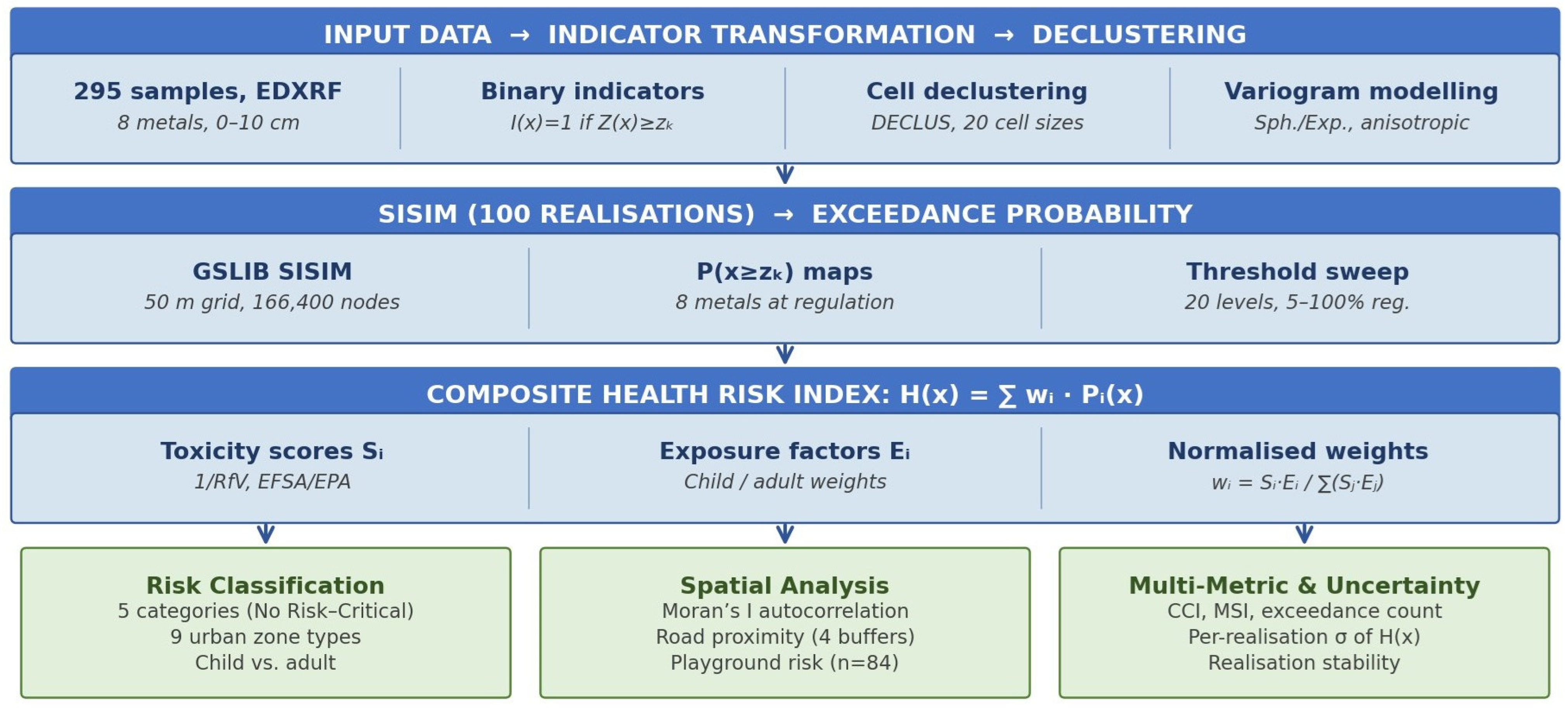
We therefore chose the previously published concentration mapping [5] as a starting point and converted the exceedance probabilities into a spatially resolved exceedance-priority indicator using stochastic simulation and toxicity-weighted composite indexing. All eight metals were related to the Hungarian regulatory action levels (Government Decree 6/2009), and the metal-specific exceedance probabilities were weighted by EFSA/EPA toxicity profiles and exposure relevance factors, with separate parameterization for children and adults. The specific objectives were as follows: (i) to generate exceedance probability maps for eight heavy metals using SISIM with 100 equiprobable realizations at Hungarian regulatory thresholds; (ii) to test whether a toxicity-weighted composite exceedance index, classified into five priority classes, provides finer spatial discrimination than single-metal exceedance maps; (iii) to evaluate the sensitivity of the exceedance area and composite index to threshold selection at 20 levels (5–100% of the regulatory value); (iv) to characterize spatial priority patterns through zone-specific analysis, spatial autocorrelation testing, road distance analysis, and sensitive receptor priority screening [21,22]; and (v) to quantify the realization-based uncertainty of the composite index across SISIM realizations [18,20] (Figure 1).
This study is distinct from the concentration mapping and source attribution of [5]: it contributes single-threshold exceedance-probability maps at regulatory limits, the toxicity-weighted exceedance-priority index H ( x ) , a threshold-sensitivity analysis, and an ensemble-convergence analysis. All analytical data are reused from [5]; no new sampling or laboratory measurement was undertaken for the present work.

2. Materials and Methods

2.1. Study Area

Debrecen is a rapidly expanding urban center located in the flat, alluvial area of the North-Eastern Great Plain (47.53° N, 21.63° E), with substantial ongoing industrial development. The city is the second largest in Hungary, with a population of approximately 200,000. The varied land use, including residential areas, transport corridors, Soviet-era industrial zones, military bases, and emerging technology parks, results in multiple pollutant sources and exposure scenarios across the study area.
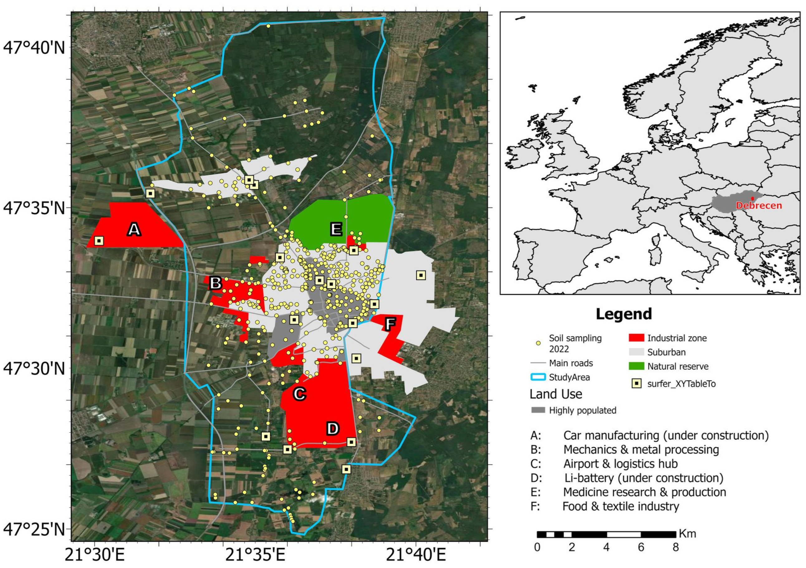
The location and extent of the study area are shown in Figure 2. It is located on a flat alluvial plain at an elevation of 110–140 m a.s.l. with Quaternary fluvial and eolian sediments. The predominant soil types include chernozoic sands in the city center and surrounding agricultural areas and sandy soils (arenosols) in the eastern and southern peripheral areas. The climate is continental, with an average annual temperature of approximately 10.5 °C and an average annual rainfall of 550 mm.

2.2. Data Set and Threshold Selection

A subset of 295 locations from the previously published sampling campaign [5] was analyzed for this study. Laboratory analyses were performed using a Skyray Instrument Explorer 9000 X-ray fluorescence (XRF) spectrometer (Jiangsu Skyray Instrument Co., Ltd., Kunshan, China) equipped with a rhodium anode X-ray tube and a silicon drift detector, the latter of which is capable of deconvoluting overlapping spectral peaks of coexisting transition metals. The samples were air-dried at 20–22 °C to constant mass, disaggregated, and sieved through a 2 mm stainless steel sieve according to ISO 11464:2006. Approximately 50 g of the <2 mm fraction per sample was measured in the factory-calibrated Soil Mode of the instrument. Each sample was measured in five independent replicates to quantify measurement precision and reduce random error, and the median of the five replicates was used for further analyses to minimize the influence of outliers. Eight heavy metals were determined: arsenic (As), cadmium (Cd), cobalt (Co), chromium (Cr), copper (Cu), nickel (Ni), lead (Pb), and zinc (Zn). Detailed sample preparation and measurement protocols are described elsewhere [5]. The 493 locations of the survey [5] form a purposively designed, multi-phase campaign. The 295 analyzed here are all available EDXRF measurements (first phase); no selection was made among measured samples on the basis of their values. The remaining 198 were sampled but not yet analyzed and are reserved for a second phase—a south-eastern expansion prompted by a recent pollution event in southern Debrecen, and a central forested/recreational belt where measurement density was deliberately reduced given its low human-exposure relevance and already-dense coverage. Their distribution is shown in Figure S1; they provide an independent validation set for a planned campaign.
The eight metals were selected based on their toxicological significance, urban occurrence, and role in national soil quality regulations. The legal action thresholds defined in the Hungarian soil quality standards (Joint Decree 6/2009 KvVM-EüM-FVM) were used as thresholds for exceedance modelling (Table 1). Descriptive statistics for the selected metals are summarized in Table 2.
The simulation grid was masked to the delineated study area boundary, resulting in an effective study area of approximately 203.2 km2. At 50 m spacing, each raster cell represents 2500 m2 (0.25 ha); grid-derived summaries are therefore reported as percentages or physical area rather than raw cell counts. The 50 m grid is a computational discretization within the range permitted by the fitted variograms, not a claim of 50 m information; effective precision is bounded by the estimation variance, which increases with distance from data (mean spacing ≈ 830 m (nominal √(A/n))). The reported quantity is the exceedance probability averaged over realizations (E-type indicator), a smooth surface. Because block indicator kriging does not yield the block ccdf, block-scale uncertainty is properly obtained by simulation [6] Equation IV.55; a grid-sensitivity check (50/100/200 m; Figure S10) confirms that exceedance areas are insensitive to discretization.

2.3. Indicator Transformation, Declustering and Variogram Modelling

Each metal concentration, Z ( x ) , was transformed into a binary indicator at the Hungarian legal threshold, z k :
I ( x ; z k ) = 1 if   Z ( x ) z k 0 otherwise
The resulting binary indicators served as inputs for variography and simulation. Each metal was represented by a single indicator at its regulatory cutoff z c ; exceedance probabilities were obtained by simple indicator kriging of that one indicator and sequential indicator simulation (GSLIB sisim, single-threshold indicator mode, one cutoff per metal). Because a single cutoff is used, one indicator variogram is fitted per metal (Table 3) and no coregionalization across thresholds is required; this single-threshold design is standard for regulatory exceedance mapping [25].
Below-detection measurements are treated as hard-inequality data [6]: for any cutoff z c set above the detection limit, the indicator I ( u ; z c ) = 0 is fully defined, not missing. For Pb (detection limit 5 mg/kg, cutoff 100 mg/kg), all 124 non-detects were therefore entered as defined zeros alongside the 171 detects, and the Pb indicator was re-run on all 295 locations; the exceedance surface is negligibly changed.
The sampling design is spatially clustered; some urban districts are over-represented compared to the rural periphery, where sampling locations are considerably sparser. Cell declustering was applied to correct this bias by assigning a weight to each observation inversely proportional to the local sampling density, thus compensating for the bias in the empirical distribution due to preferential sampling. The cell size ranged from 100 m to 5000 m, with 20 cell size steps and five origin offsets. The declustered cumulative distribution function (CDF) was calculated at each threshold as follows:
F ( z k ) = w α · I x α < z k   w α
where w α are the declustering weights.
The spatial continuity of the binary indicators was characterized by the indicator semivariogram [25].
γ I ( h ) = 1 2 N ( h ) α = 1 N ( h ) [ I ( x α ; z k ) I ( x α + h ; z k ) ] 2
where N ( h ) is the number of data pairs separated by the lag vector h . Experimental indicator variograms for each metal were computed and fitted with spherical or exponential models with geometric anisotropy (Table 3).
Experimental indicator variograms were computed omnidirectionally with a lag spacing of 500 m and 12 lags to ~ 1.5 × the fitted range, checked for anisotropy along the principal directions, and fitted by weighted least squares with visual verification. The declustering cell size (100–5000 m; 20 sizes, 5 offsets) and its effect on the declustered marginal proportions are reported in Supplementary Table S9. Experimental and fitted variograms are shown in Figure S7.

2.4. Sequential Indicator Simulation and Exceedance Probability

The sequential indicator simulation (SISIM) was used to generate 100 equiprobable realizations of the spatial distribution of threshold exceedance (4–12 neighborhood, search ellipsoid matched to variogram model) [6,17]. The ensemble size was selected on the basis of a convergence analysis in which SISIM was run at seven ensemble sizes ( N   =   10 ,   25 ,   50 ,   100 ,   200 ,   500 ,   1000 ) for all eight metals (Table S4, Figure S3a,b, Supplementary Materials). At N   =   100 , binary exceedance classification agreed with the N   =   1000 baseline to within 1% for seven of the eight metals: As, Co, Cu, Ni, Pb, and Zn converged at N   =   10 25 , and Cd at N   =   100 . Only Cr, whose indicator proportion lies near 0.50 (52.3%), showed slower convergence and was regenerated at N   =   1000 , where its p   >   0.50 exceedance area is ≈82% (from ≈61% at N   =   100 ); because Cr contributes only 0.007% of the H ( x ) weight, the composite ranking is unaffected. Supplementary Text S4 explains the pixel-level versus areal convergence and the ergodic (Monte-Carlo) origin of the near-boundary residual.
SISIM was chosen over sequential Gaussian simulation (SGS) because it does not require the multi-Gaussian condition, weakens the stationarity assumption to the binary indicator field, and avoids normal-score transformation problems where observations lie near detection limits [6,18,19,20]. The theoretical rationale and comparison with kriging, SGS, and machine learning point prediction are summarized in Section 4.4 and given in full in Supplementary Text S1.
The eight metals were simulated independently, without co-simulation. This simplification is partly supported by the inter-metal correlation structure and factor analysis groupings [5] and is reproduced for traceability in Tables S1 and S2a,b (Supplementary Materials). The source factor analysis was acceptable for interpretation ( K M O   =   0.618 ;   χ 2 =   416.463 ,   p   <   0.001 ) . Although the continuous concentrations of As and Cd are moderately correlated (Spearman   r   =   0.80 ), their indicator variables at the respective regulatory thresholds are weakly correlated (indicator Spearman r   =   0.24 ), because the exceedance proportions are far apart (As: ~12% raw sample exceedance, Cd: 81%) and the threshold-specific spatial structures differ. The metals most strongly correlated with As and Cd in continuous space (Zn: r   =   0.94 and r   =   0.77 ; Pb: r   =   0.83 and r   =   0.59 ) have near-zero exceedance probabilities at the regulatory thresholds, so this cross-correlation does not propagate into the composite index. Co-simulation was therefore not pursued; its effect on the composite ranking would be negligible given the weak indicator-level dependence between the two metals that account for 88% of the H(x) weight.
The indicator-level dependence between the two dominant metals is weak (Spearman r   =   0.24 ) even though their concentrations are correlated ( r   =   0.80 ); a multivariate/compositional treatment is therefore not adopted, as each element is assessed against its own absolute regulatory limit rather than under closure, and full indicator cokriging is impractical and offers little gain here [6].
For all x 0 locations not coinciding with sampling locations, the conditional probability of exceedance is estimated by simple indicator kriging:
P x 0 z k   |   d a t a   = λ α · I x α ; z k + 1 λ α · F z k
where λ α are the kriging weights derived from the fitted indicator variogram, and F z k is the declustered global CDF. Simple kriging was used because the global mean proportion is known from declustering and because SK produces more stable local probability estimates than ordinary kriging in the SISIM framework [26].
SISIM can result in non-monotonic conditional CDF estimates when multiple thresholds are applied simultaneously, which is a known order-relation violation [18]. In the present application, all metals were simulated at a single legal threshold, which circumvents the multi-threshold CDF problem.
For each grid node x , the exceedance probability was estimated as the proportion of exceedances across realizations:
P ( x z k ) = 1 L l = 1 L I l ( x ; z k )
where L = 100 is the number of realizations, and I l ( x ; z k ) is the simulated indicator value at location x in the l -th realization. These probabilities express local uncertainty and range from 0 (no exceedance in any realization) to 1 (exceedance in all realizations), but do not capture the spatial covariance of exceedance between neighboring nodes. We applied the confidence classification of Van Meirvenne and Meklit [19]: exceedance probabilities below 0.25 indicate high certainty of non-exceedance, the range 0.25–0.75 indicates a transition zone where the classification outcome is ambiguous, and probabilities above 0.75 indicate high certainty of exceedance. The transition zone identifies sites where additional sampling would most effectively reduce classification uncertainty.
The simulation assumes second-order stationarity of the indicator field within the study area; this is a modelling assumption, not a verified property of the contamination field [18]. All metals were simulated independently; the eight indicator fields did not share a common co-simulation model, and potential spatial cross-correlations between metals were not reproduced. Consequently, the composite index sums the marginal exceedance probabilities, not the joint probabilities.

2.5. Composite Exceedance Index

To integrate multi-metal exceedance into a single spatial index, we defined a composite index, H ( x ) , which aggregates toxicity-weighted exceedance probabilities across metals. H ( x ) is a toxicity-weighted exceedance index that ranks sites according to the combined probability of exceeding regulatory limits. It is not a health risk index in the epidemiological sense of the hazard quotient ( H Q ) or hazard index ( H I ). Arsenic and cadmium account for ≈88% of the child-scenario weight; H ( x ) is therefore, by design, dominated by the two most toxic and bioavailable elements. The rank correlation between H ( x ) and a pure As + Cd index is ρ = 0.998 ; only 1.9% of the study area changes priority class once the other six metals are included, and those cells are mapped in Figure S9. The per-metal reference values, their type and source, and the assigned exposure-relevance factors are tabulated for transparency in Supplementary Table S8.
H ( x ) = i = 1 8 w i · P i ( x )
where P i ( x ) is the exceedance probability of the i -th metal, w i is the normalized weight, and the summation extends over all eight metals. The index was calculated separately for children and adults to reflect their differential exposure. The hazard quotient ( H Q ) and hazard index ( H I ) [27] have been widely used for deterministic risk estimation from point concentration estimates, and the potential ecological risk index ( P E R [28]) uses concentration ratios [29]. We note that H ( x ) is distinct from both indices because it applies weights to exceedance probabilities rather than to concentration ratios, thereby incorporating simulation-based uncertainty directly into the priority ranking [7]. These two approaches are complementary, not competing.
Toxicity scores S i were derived as reciprocals of chronic oral reference values:
S i = 1 R f V i
where R f V i is the reference value in mg/kg/day. Reference values were obtained primarily from the European Food Safety Authority (EFSA), supplemented by reference doses (RfD) from the US Environmental Protection Agency (US EPA) where EU values were not available. The toxicity scores cover four orders of magnitude: arsenic ( B M D L 01   =   0.0003   m g / k g / d a y ,   S   =   3333 ; [30]) and cadmium ( T W I   =   0.001   m g / k g / d a y ,   S   =   1000 ; [31]) dominate, followed by cobalt ( 0.003   m g / k g / d a y ,   S   =   333 ; [32]) and lead ( T W I   =   0.0035   m g / k g / d a y ,   S   =   286 ; [33]). Nickel ( A R f D   =   0.02 ,   S   =   50 ; [34]), copper ( U L   =   0.04 ,   S   =   25 ; [35]), and zinc ( U L   =   0.3 ,   S   =   3.3 ; [36]) were minimal contributors. Cr received the lowest score of 0.67 ( R f D   =   1.5 ; [37]). This low score reflects the fact that only the less toxic Cr(III) form was considered in the derivation of the reference dose. In urban soils, a fraction of total chromium exists as the more toxic Cr(VI) form, but this dataset contains total Cr only and no Cr speciation; Cr(VI) was therefore handled through scenario analysis. Because Cr(VI) has an oral RfD of 0.003 mg/kg/day ( S   =   333 ), even a small Cr(VI) fraction increases the effective toxicity score. A sensitivity analysis evaluating the impact of 5% and 10% Cr(VI) fractions on the composite index is presented in Supplementary Text S3 (Table S5, Figure S4, Supplementary Materials).
The toxicological reference values, exposure relevance factors, and resulting normalized weights for both children and adults are given in Table 4; the child/adult exposure distinction follows standard exposure-factor guidance [38].
Ei values were assigned following the ECHA tiered exposure pathway framework [39]: 1.00 for metals with a dominant oral–soil pathway in children (As, Cd, Pb), 0.75 for metals with secondary dermal or inhalation routes (Co, Cu, Ni), and 0.50 for metals where dietary intake exceeds soil-mediated exposure (Cr, Zn).
w i = S i × E i j = 1 8 S j × E j
Complementary unweighted multi-metal indices (cumulative contamination index, CCI; multi-metal contamination severity index, MSI) were also computed from the SISIM exceedance probabilities to capture co-occurrence patterns that are masked by toxicological weighting; their definitions and spatial distributions are provided in Supplementary Text S2.

3. Results

3.1. Exceedance Probability Maps

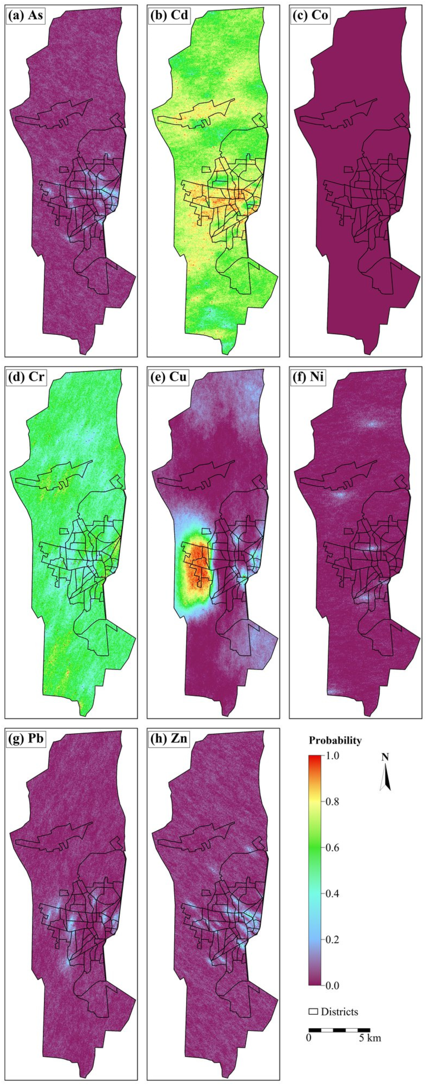
The exceedance probability maps for the eight heavy metals were generated from 100 SISIM realizations on the 50 m simulation grid (Figure 3). Each map shows the probability that the Hungarian legal action level is exceeded at a given location (Table 5). All exceedance probabilities are at point support; the 50 m cell size is a computational discretization of the continuous indicator field, not a block-averaged estimate. Block-support exceedance probabilities would be lower owing to the regularization effect [17,20].

3.2. Threshold Sensitivity Analysis

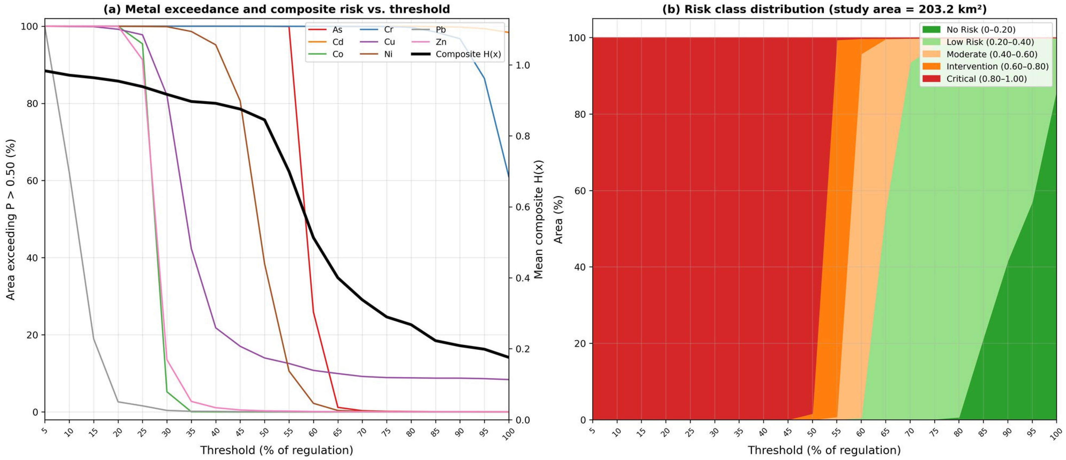
To examine the threshold dependence of the exceedance area, a systematic threshold sensitivity analysis was performed at 20 levels (5–100% of the Hungarian action threshold with a step size of 5 percentage points) (Figure 4). The results allow the identification of three distinct metal response types.
The exceedance area for Cd remained above 98% over the entire threshold range at p   >   0.50 . The near-universal exceedance of Cd reflects a regulatory limit (1 mg/kg) set below the median concentration (1.33 mg/kg). The mean exceedance probability for the study area was 0.692, indicating that individual grid cells are not uniformly contaminated, but the proportion of the study area where exceedances were observed in the majority of realizations is nearly universal.
Arsenic, chromium, copper, and zinc are threshold-sensitive metals. The exceedance area decreased markedly with increasing threshold level, following characteristic S-curves with inflection points at metal-specific positions. Arsenic decreases from nearly 100% to nearly 0% between 55% and 70% of the regulatory level (about 8.2–10.5 mg/kg), while chromium decreases more gradually from 100% (at the 50% level) to about 82% (at the 100% level), the latter regenerated at N   =   1000 (Table S4). The exceedance classification of these metals exhibits pronounced threshold dependence, reflecting the choice between regulatory action limits and lower screening values.
Cobalt showed no exceedance at the regulatory limit. Nickel had rare sample-level exceedance (6/253 samples; 2.4%) but produced a spatially negligible mapped exceedance area at p   >   0.50 , so neither Co nor Ni materially contributes to H ( x ) at the regulatory thresholds.
The composite H ( x ) decreased monotonically from about 0.94 at 25% of the regulatory limit to about 0.205 at 100%, reflecting the overall threshold sensitivity of the contamination field. The steepest decline occurred between 50% and 80%, where the threshold sensitive metals transitioned from widespread to localized exceedance.

3.3. Composite Exceedance Index and Priority Classification

The composite exceedance index (Equation (6)) was calculated for both children and adults at the regulatory thresholds. The average H ( x ) for children was 0.205 across the modelled area. The higher composite values were mainly concentrated along major transport corridors, older residential areas, and public playgrounds, consistent with previously identified pollution sources [5]. For adults, the average H ( x )   =   0.179 , a difference of less than 2%. These differences presumably reflect the fact that arsenic and cadmium, which dominate the composite index, receive the same normalized weights for children and adults, while lead, which shows the largest child–adult weight difference, has a near-zero exceedance probability and therefore contributes negligibly to H(x) regardless of exposure weighting. Since the child and adult indices are nearly identical, the results below are presented for children only.
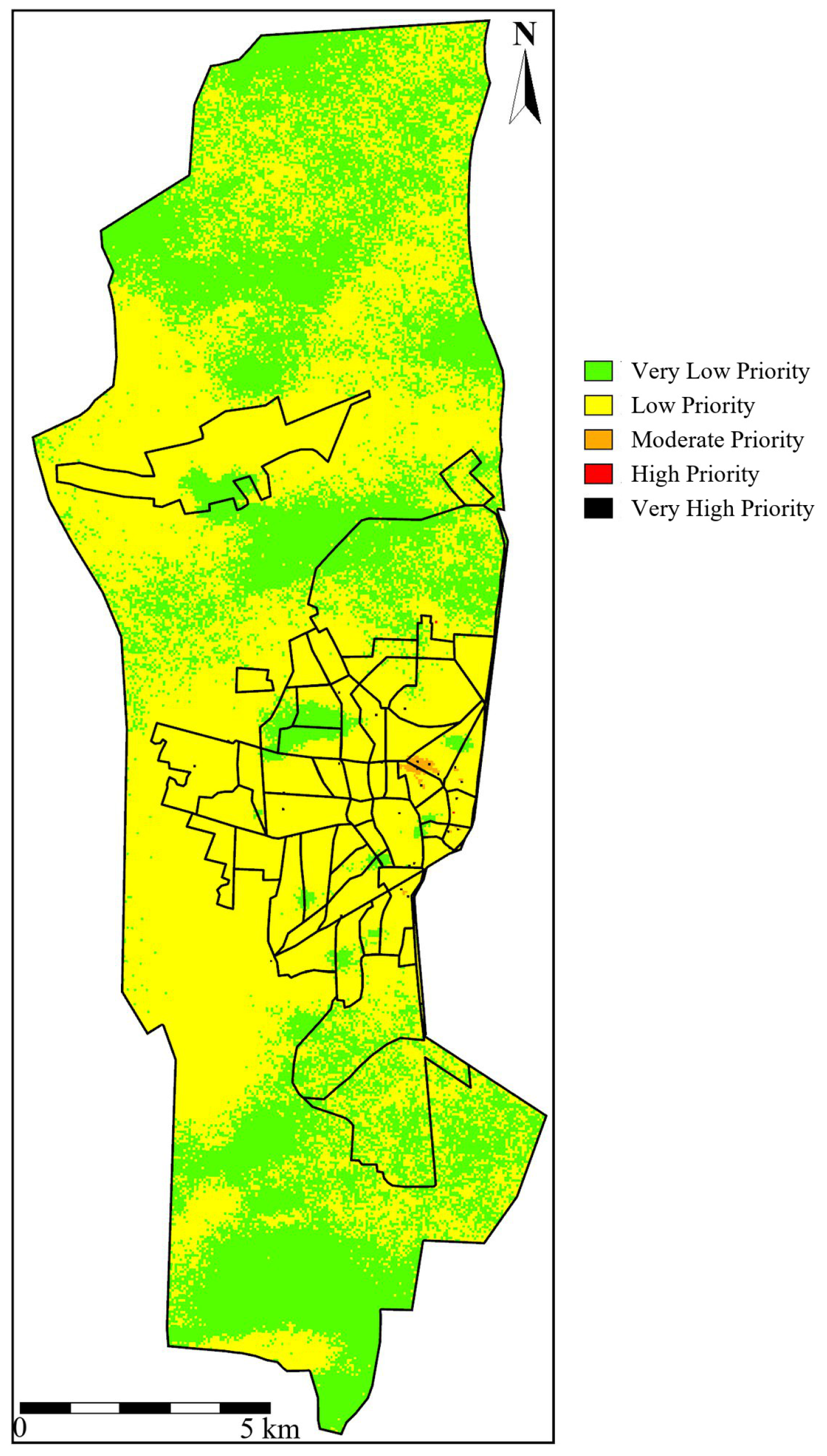
We classified the values of the composite exceedance index H ( x ) into five priority classes (Table 6, Figure 5).
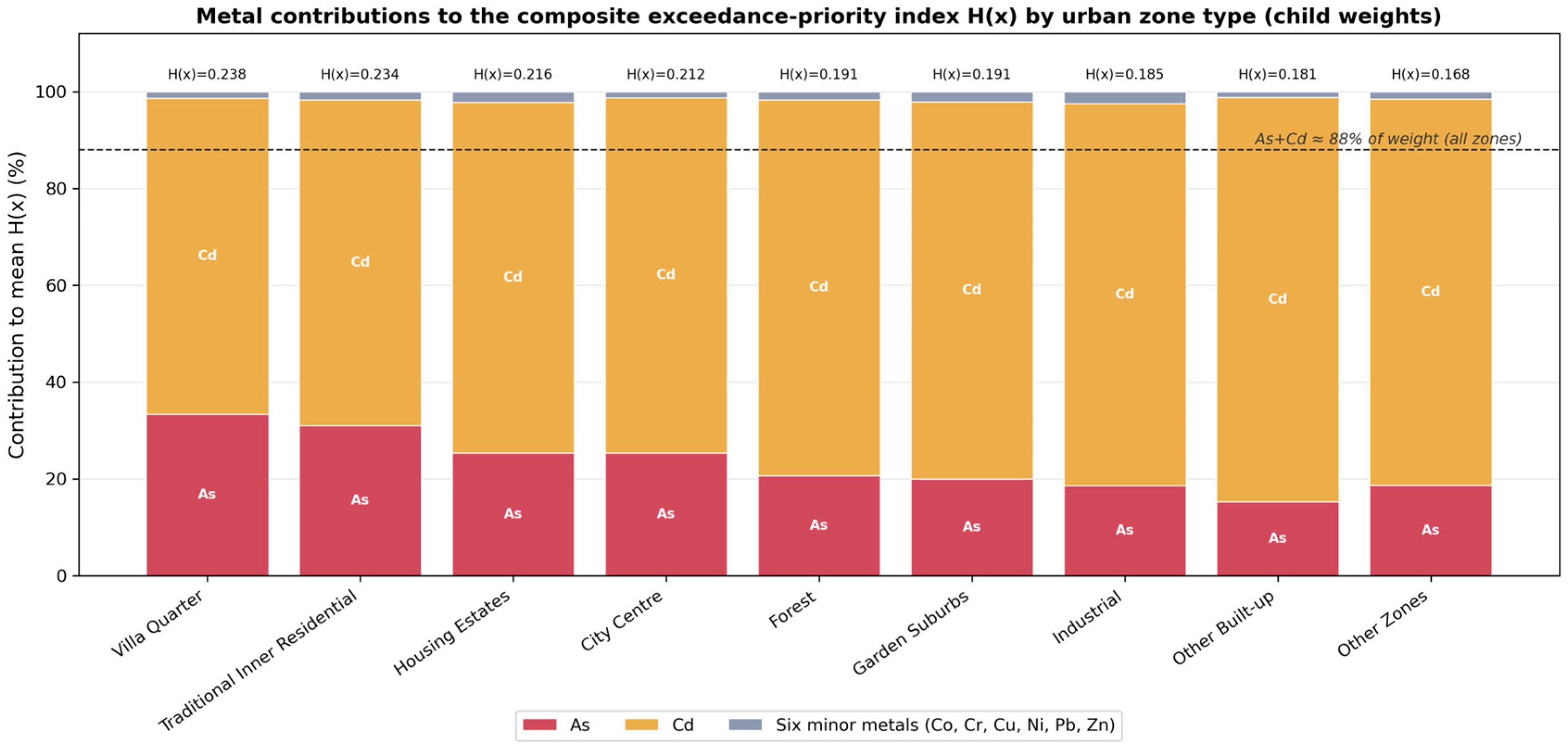
Metal-specific contributions to H ( x )   by urban area type are shown in Figure 6.

3.4. Zone-Specific Patterns and Spatial Autocorrelation

The average H(x) varies across the nine urban area types (Table 7).
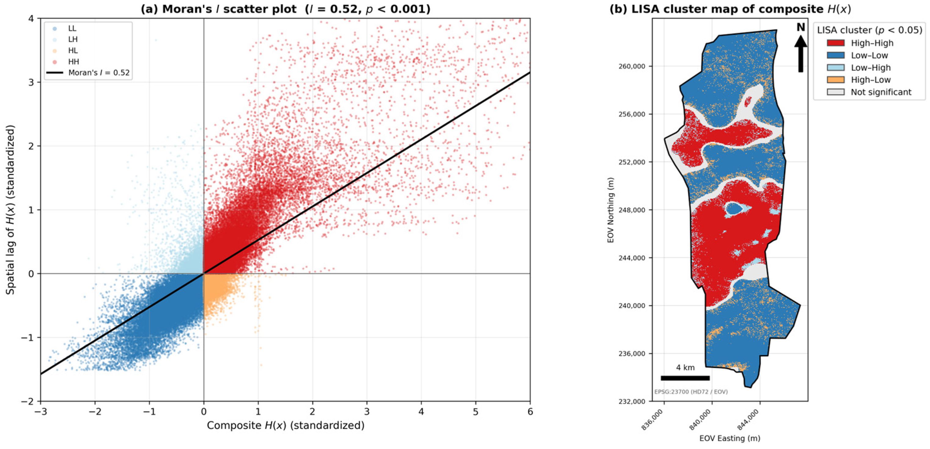
The global Moran’s I for the composite H ( x )   was 0.52 ( p   =   0.001 , 999 permutations; row-standardized distance-band weight of ~700 m, corresponding to the mean sample spacing), confirming statistically significant positive spatial autocorrelation; high-priority grid cells cluster together and so do low-priority cells (Figure 7). The LISA cluster map [40] identifies a persistent High–High cluster in the east-central residential area, coinciding with the four sensitive receptors flagged in Section 3.6.

3.5. Road Distance Analysis

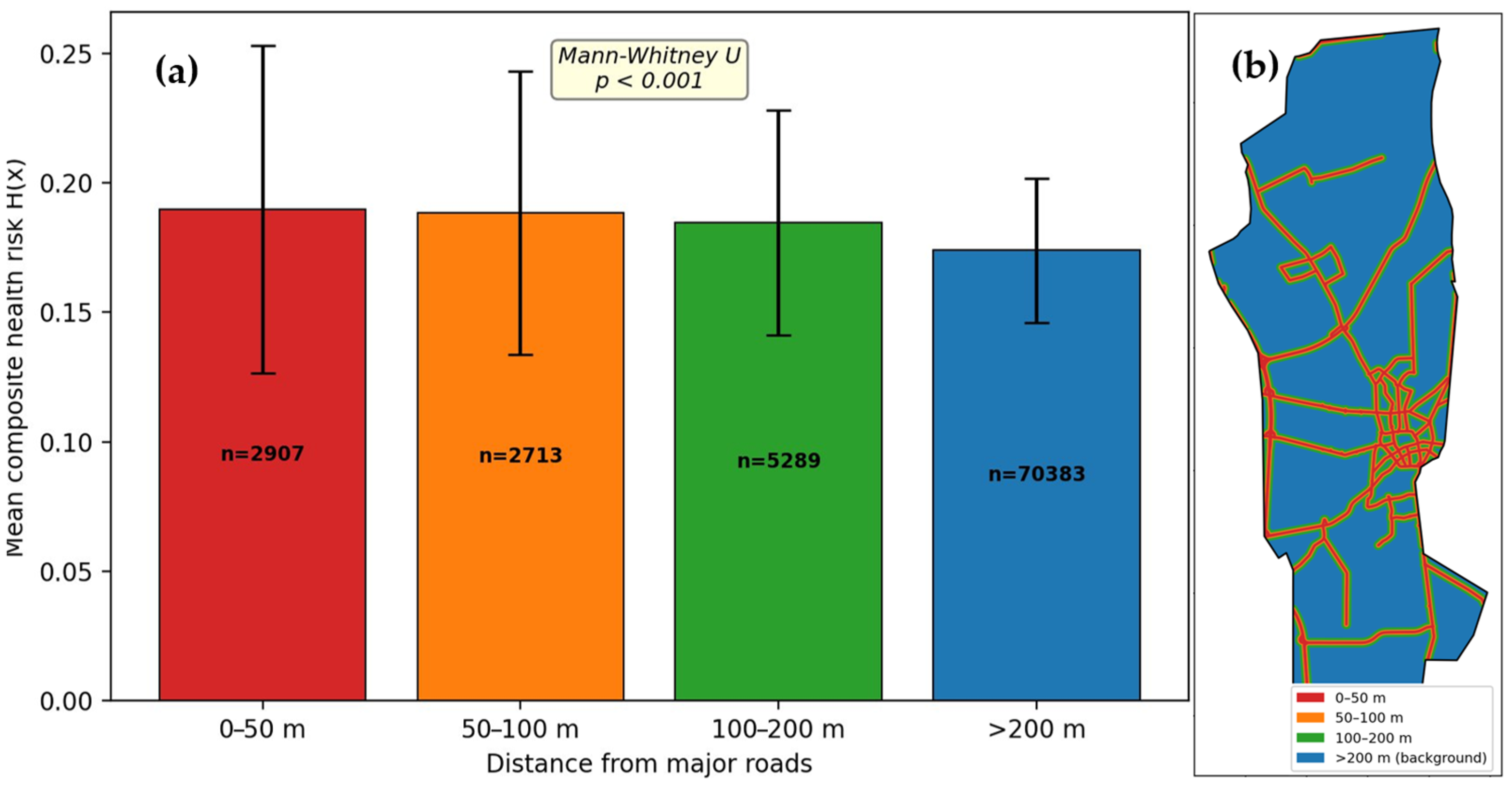
The average H ( x ) decreased gradually from the primary and secondary roads towards the background (approximately 1000 road segments; Figure 8, Table 8).

3.6. Sensitive Receptor Assessment

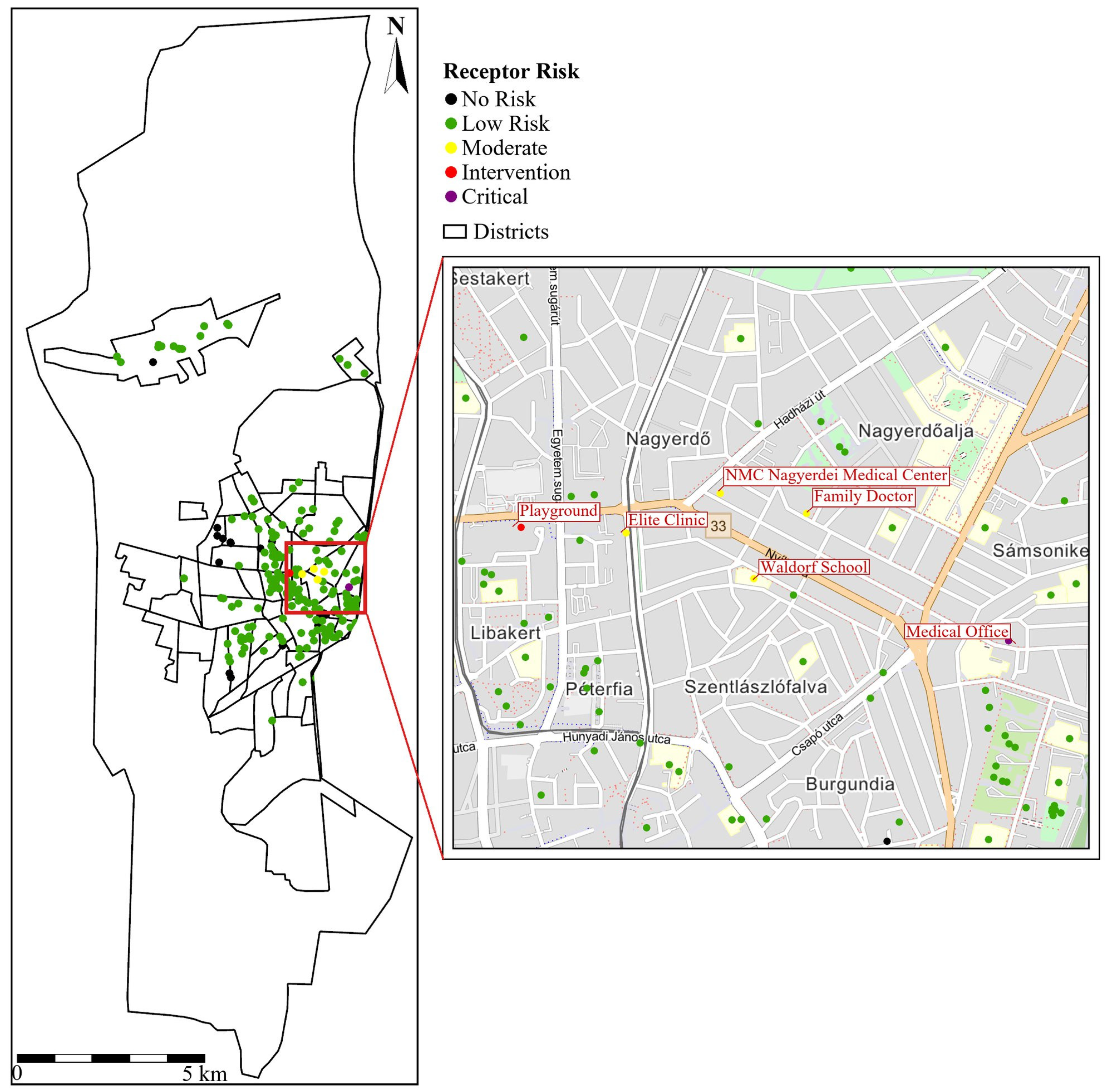
A total of 208 sensitive receptors (84 playgrounds, 65 schools, 28 kindergartens, and 31 childcare and health care facilities) were identified in the study area based on OpenStreetMap (Figure 9). The composite exceedance index H(x) of each receptor was classified into five priority categories.
The H(x) values of the receptors were at the Very Low Priority ( H   <   0.20 ) or Low Priority ( H   =   0.20 0.40 ) level, with the exception of four receptors that exceeded the Moderate Priority threshold ( H   >   0.40 ): one nursery school (Very High Priority, H   =   0.94 ), one playground (Very High Priority, H   =   0.88 ), one childcare facility (Moderate, H   =   0.45 ), and one school (Waldorf School, Moderate Priority, H   =   0.41 ). All four high-priority receptors were concentrated in the east-central area of Debrecen.
The elevated H(x) estimated at the highest priority receptor (a nursery school, H   =   0.94 ) is associated with the combined elevated probabilities of arsenic and cadmium exceedances. Because children are more susceptible to the toxic effects of heavy metals, the four facilities in the urban core warrant confirmatory soil sampling to determine whether these values reflect true contamination or simulation uncertainty, while the vast majority of sensitive receptors require routine monitoring at most.

3.7. Uncertainty, Multivariate Indices and Validation

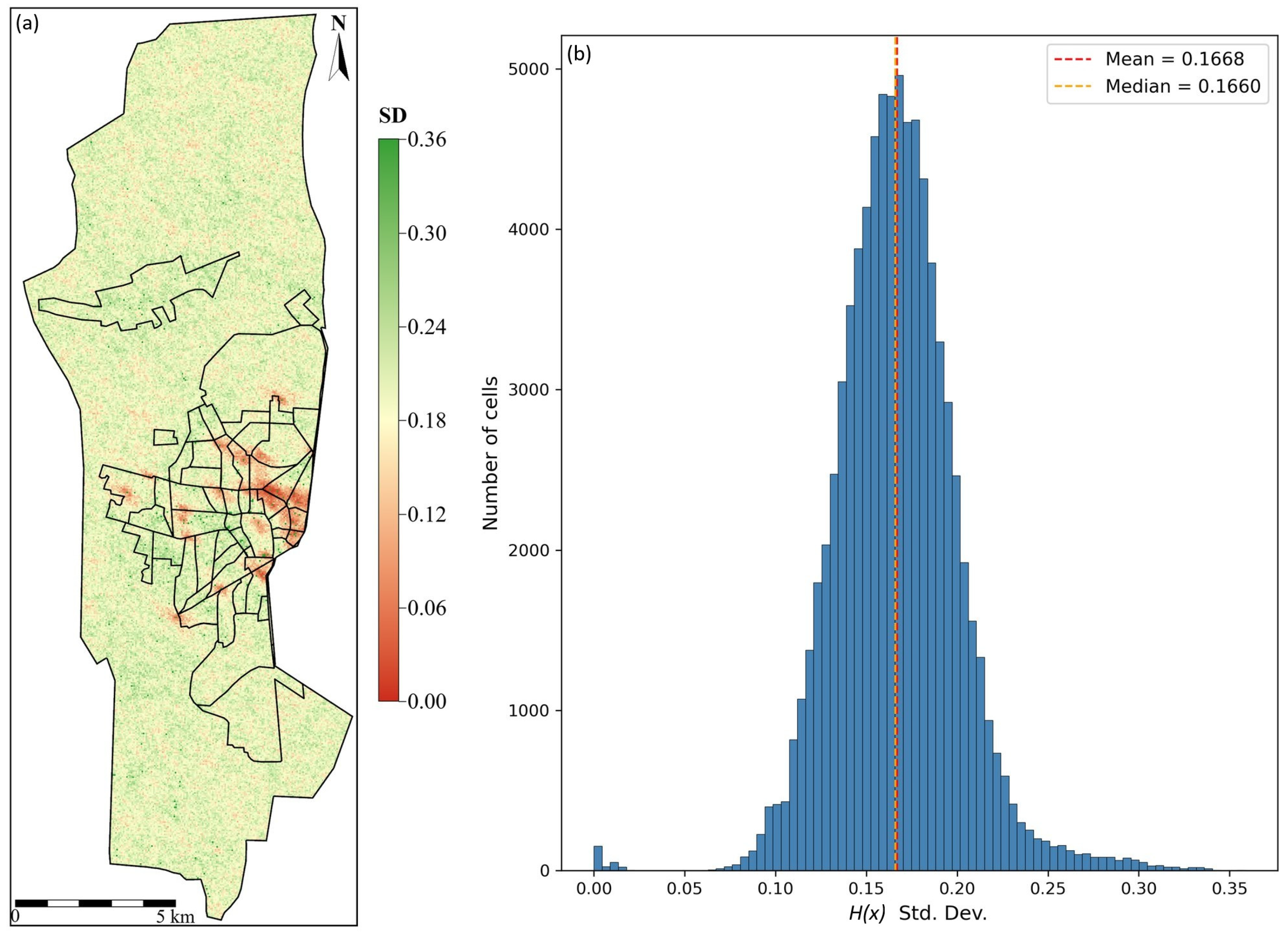
The unweighted CCI and MSI indices confirmed multi-metal co-occurrence in the urban core and finer spatial differentiation than the toxicity-weighted H ( x ) ; cobalt and nickel did not contribute at the regulatory thresholds. Definitions and statistics for CCI and MSI are provided in Supplementary Text S2, and the corresponding maps are shown in Figure S8. Realization-level uncertainty is shown in Figure 10.
Internal consistency was checked by comparing the per-realization mean of H ( x ) to the probability-based estimate. The average absolute difference was 0.029 (100 realizations). A comparison of 10-realization debug runs and 100-realization production runs reveals the practical consequence of an insufficient number of realizations. The average exceedance probabilities are stable across ensemble sizes (deviations < 0.01), but the binary classification at p   >   0.50 is sensitive: the exceedance area for cadmium increased from about 81% (10 realizations) to about 98% (100 realizations), and that for chromium from about 44% to about 61%. This sensitivity arises because grid nodes with a posterior probability near 0.50 lie in the transition zone, where the binary classification oscillates as additional realizations push the ensemble proportion over the decision threshold.
The Monte Carlo sensitivity analysis showed that the spatial ranking of H ( x ) was robust to simultaneous perturbation of all child exposure relevance factors (Table S3 and Figure S2, Supplementary Materials). Across 1000 iterations, the median Spearman rank correlation between baseline and perturbed H ( x )   was 0.989 ( I Q R   =   0.967 0.997 ), and the mean absolute H ( x ) difference was 0.0336. Approximately 25.6% of grid cells changed priority category, but this should be interpreted in relation to the low baseline mean H ( x ) and the dominant Very Low Priority/Low Priority boundary at   H ( x )   =   0.20 : many cells lie close to this boundary, so small absolute shifts can change class without altering the broader spatial priority pattern.
The SISIM outputs were validated against three criteria. The average simulated exceedance rates for all metals were within 2% of the declustered observed rates. The indicator variograms of 50 randomly selected realizations reproduced the fitted variogram models within acceptable tolerances; a visual comparison of the experimental omnidirectional indicator variograms and the fitted models for all eight metals is provided in Figure S7 (Supplementary Materials). The spatial patterns of the realizations showed a distribution consistent with known pollution sources and land use.
The stratified 10-fold cross-validation showed a mean accuracy of 0.87 and mean A U C of 0.68 across the eight metals (Table S6, Figure S5, Supplementary Materials). Co had perfect accuracy but undefined A U C because no sample exceeded the 30 mg/kg regulatory threshold. Ni had high accuracy (0.976) but low A U C (0.514) and zero sensitivity because only 6 of 253 samples exceeded the 40 mg/kg threshold. These results support interpretation of the SISIM outputs as probability surfaces rather than deterministic classifications, especially for rare-exceedance metals.

4. Discussion

4.1. Contamination Profile and Priority Classification

The widespread exceedances of cadmium and chromium arise from different mechanisms for each metal. The high nugget/sill ratio of Cd (0.68; Table 3) indicates a high degree of short-range spatial variability and that about 68% of the indicator semi-variance at the smallest lag distance remains unresolved. This variability is physically present in the soil below the median nearest-neighbor sampling distance of 180 m but cannot be resolved by the sampling grid [18]. SISIM carries this unresolved variability forward into the conditional probability at each grid node, presumably because kriging provides a smoothed estimate that systematically underestimates the proportion of extreme values, i.e., the smoothing effect. Goovaerts [7] showed that indicator simulation reduced the cost of misclassification by 18% on average per site compared to ordinary kriging. Chromium concentrations were close to the regulatory threshold (median 62.9, limit 75 mg/kg), so that a large part of the study area falls within the transition zone, where the posterior probability is most sensitive to the local conditioning configuration.
According to the Geochemical Atlas of Hungary [23], Cd geochemical background is low—expected value < 0.5 mg/kg—both below the 1 mg/kg regulatory threshold, so the widespread Cd exceedance is not an artefact of a sub-background limit. The Debrecen median (1.33 mg/kg) exceeds the expected background and the threshold (though within the broad regional characteristic range up to ≈1.5 mg/kg), indicating genuine moderate Cd enrichment (mixed lithogenic and diffuse anthropogenic, per [5]). Because near-threshold Cd values approach the XRF detection limit (2 mg/kg), the exceedance magnitude should be read as an enrichment indicator rather than a precise measurement.
Because only total Cr was measured, H ( x )   is not intended for Cr-specific health-risk inference; areas of elevated total Cr near sensitive receptors may warrant confirmatory Cr(VI) analysis. The Cr(III)/Cr(VI) scenarios (Supplementary Table S5, Figure S4) are bounding cases, not a speciation model.
The supplementary SISIM–OK comparison (Figure S6, Table S7) was recomputed with a numerically stable ordinary-kriging solver. SISIM and OK classifications agree for most metals (≥96% for six of eight); they diverge only where the median concentration lies near the regulatory threshold—chromium (SISIM ≈78%, OK ≈80% in this N   =   100 benchmark) and copper, where OK smoothing over-calls exceedance (OK 48% vs. SISIM 4%). The smoothing effect is therefore distribution-dependent rather than uniform and is most consequential for metals whose median sits close to the regulatory limit.
Compared to the previous characterization of Debrecen soils [5], where cobalt and nickel were identified as contaminants, Co does not exceed the legal limit, while Ni exceedance is rare (6/253 samples; 2.4%) at the 40 mg/kg threshold. Co and Ni were identified as contaminants in the previous characterization because the thresholds applied were approximately the median concentrations in the data set, while the regulatory action thresholds were not applied [5]. When the concentrations of Co and Ni are compared with the regulatory thresholds, the determination of soil contamination can be misleading without an appropriate threshold, and this is what the threshold sensitivity analysis makes explicit.
A cut-off of H ( x )   =   0.20 separates the two dominant categories and is approximately the level at which two metals simultaneously reach or exceed their legal limit. Because the class boundaries are a classification convention and not dose-response thresholds, this division should be interpreted as a relative ranking in the contamination assessment, consistent with the Monte Carlo sensitivity result in Table S3.

4.2. Threshold Sensitivity

The three response types identified in Section 3.2 imply that the exceedance area and the composite H ( x )   are not stable properties of the contamination field, but are a function of the chosen threshold. Although studies that report exceedance results at a single threshold implicitly assume stability, the threshold area curves show that for several metals (As, Cr, Ni), a 10-percentage point threshold shift can cause a 20–40 percentage point change in the exceedance area. Evaluations that do not characterize this dependence are vulnerable to threshold revisions.

4.3. Spatial Patterns: Zones, Pathways, and Sensitive Receptors

Composite H ( x ) was higher in residential zones than in industrial zones (Table 7) because the composite index combines exposure relevance and toxicity weights, so that the same level of contamination leads to a higher H ( x ) priority score where children actually reside. The results indicate that the dominance of cadmium in all zone types (65–84%), combined with the secondary role of arsenic (15–34%) in residential areas, results in elevated exceedance probabilities. Whether this overlap reflects a common source or a spatial coincidence cannot be determined from the available data, and source apportionment analysis would be needed to resolve the multi-metal spatial co-occurrence patterns.
The H(x) priority pattern is validated against the independent anthropogenic source factor of [5] (Factor 1: log As, log Pb, log Zn, Co): the two correlate significantly (Spearman ρ   =   0.51 ,   p   <   0.001 ; Figure S11), confirming that high-priority zones coincide with documented contamination sources. The 198 reserved locations additionally constitute a prospective out-of-sample validation set for a planned campaign. These are corroborative, not confirmatory.
Heavy metal contamination of roadside soils was associated with localized point source emissions at specific locations, consistent with the previous identification of traffic as the dominant contamination source in Debrecen [5]. The receptor-focused interpretation is also consistent with studies documenting heavy metal contamination in child-sensitive urban settings such as parks, playgrounds, and preschool facilities [41,42]. Increasing variance near roads is consistent with spatially heterogeneous contamination rather than a uniform roadside band.
The four high-priority receptors (Section 3.6) warrant careful interpretation, as H(x) for a single receptor site is a point-support estimate on a 50 × 50 m grid cell, while the physical extent of a playground or school building corresponds to a block-support volume. Regularization to block support reduces the dispersion variance and consequently reduces the exceedance probability relative to the point-support value [20]; the reported H(x) values at these receptors are therefore upper bounds on the block-support H(x). The conditional probability at any given grid node also depends on the visiting-order of the sequential algorithm; different random visiting sequences result in different conditioning configurations and hence different local posterior distributions [26]. This path-order dependence is most pronounced for indicator categories with low global proportions: in this study, Ni (2.4%), Pb (4.3%), and As (4.7%). The conditioning density of the 295 observations on the approximately 203 km2 study area is sparse, and the uncertainty at any given receptor site depends on the local data configuration and the range of the indicator variogram [43]. The four high-priority receptors may therefore reflect true localized contamination but may equally reflect stochastic fluctuations at data-poor sites. The costs of misclassification are asymmetric; under-prioritizing a truly contaminated site has larger public health consequences than flagging a site for confirmatory sampling [7]. Confirmatory sampling of these four sites is warranted before remediation decisions are made.

4.4. Methodological Comparison with Alternative Approaches

The choice of SISIM over alternative spatial prediction methods rests on four properties that are important for regulatory exceedance mapping and are discussed in detail in Supplementary Text S1. First, kriging minimizes local estimation variance but suppresses extremes, which can bias exceedance probabilities downward at the locations where contamination is highest [7,20]. Second, sequential Gaussian simulation requires the multi-Gaussian condition, which is difficult to justify for skewed heavy-metal data and can decorrelate extreme values [6,8,20]. Third, SISIM constrains stationarity to the binary indicator field rather than the continuous concentration surface, which is more defensible in heterogeneous urban soils [6,17,44]. Fourth, standard machine-learning point-prediction workflows do not directly provide the spatially coherent multi-site uncertainty required for area-based remediation decisions or for propagating uncertainty through H(x) [8,45,46].
An empirical ordinary-kriging comparison on the present dataset is useful as a cautionary check but should be interpreted conservatively (Table S7, Figure S6). For Cd, where exceedance is widespread, OK and SISIM agreed closely. For Cr, SISIM produced a much larger exceedance area than OK, consistent with the known smoothing effect. For several metals with sparse or no exceedances, however, auto-fitted OK variograms produced physically implausible predictions, including negative mean concentrations for Co, Cu, and Pb and an extreme overestimate for Ni (OK mean = 783 mg/kg against a 40 mg/kg threshold). These artifacts show why continuous OK with automatic variogram fitting is not a defensible replacement for threshold-targeted SISIM in this dataset; the SISIM probability surfaces based on expert-fitted indicator variograms remain the primary results.

4.5. Uncertainty and Methodological Context

The conditional variance of H ( x ) over the 100-realization ensemble (mean standard deviation = 0.167; Section 3.7) implies that nodes near the Very Low Priority/Low Priority boundary ( H   =   0.20 ) can migrate between categories across realizations. The Monte Carlo analysis of exposure relevance factors leads to the same practical interpretation from a different uncertainty source; rank correlations remained very high, but categorical assignments near H ( x )   =   0.20 changed for a substantial fraction of cells (Table S3, Supplementary Materials). The transition zone is where additional sampling would most effectively reduce misclassification uncertainty [18,19,20]. The sensitivity of binary classification to the ensemble size between 10 and 100 realizations (Section 3.7) falls within the range where the average exceedance rate converges rapidly, suggesting that the area classified as exceeding the threshold at p   >   0.50 remains unstable until the ensemble is large enough to resolve the conditional probability at nodes near p   =   0.50 .
A systematic convergence analysis confirms and extends this observation (Table S4, Figure S3a,b). SISIM was run at seven ensemble sizes ( N   =   10 ,   25 ,   50 ,   100 ,   200 ,   500 ,   1000 ) for all eight metals. Seven of the eight metals reached <1% misclassification relative to the N   =   1000 baseline at N     100 . Metals with extreme indicator proportions—As (4.7%), Co (0.0%), Cu (18.3%), Ni (2.4%), Pb (4.3%), and Zn (5.4%)—stabilized at N   =   10 25 because most locations lie far from the p   =   0.50 decision boundary. Co converged trivially because the maximum observed concentration (23.9 mg/kg) is below the regulatory threshold (30 mg/kg), so the exceedance probability is zero everywhere. Ni similarly converged at N   =   10 with 100% classification agreement at N   =   100 because only 6 of 253 samples exceeded the 40 mg/kg threshold. Cd converged at N   =   100 (0.7% misclassification). Only Cr (indicator proportion 52.3%) showed slower convergence, with 29.1% misclassification at N   =   100 and N   >   500 required to fall below 1%. This behavior is consistent with binomial sampling theory near p   =   0.50 . Composite H(x) priority classification changes were concentrated at the Very Low Priority/Low Priority boundary and did not alter the spatial priority ranking.
There are known theoretical limitations of the SISIM framework that affect the interpretation of these uncertainty estimates; these can be traced back to the restrictive conditions on the exact reproduction of indicator correlograms, which are usually not satisfied in two or more dimensions [18]. In practice, realizations should be treated as stochastic images rather than draws from a fully specified probability model [18]. The posterior probability of an event for a given node also depends on the grid resolution and the size of the simulated domain, both of which are user-defined. These caveats do not invalidate the ensemble statistics but imply that the uncertainty estimates are themselves model-dependent approximations. The uncertainty estimates in the present study reflect the inherent properties of the SISIM framework, including the path dependence of the sequential simulation algorithm and the sensitivity of exceedance rates to conditioning data density [26]. The path dependence is most pronounced for the indicator categories with low global proportions, suggesting that Ni (2.4%), Pb (4.3%), and As (4.7%) are the metals most affected in the present study.
These results are consistent with other urban soil studies in Central and Eastern Europe. Rapant et al. [47] identified arsenic as the primary contaminant of concern in Slovak urban soils, with the exception that cadmium dominated in Polish industrial zones [48]. The combination of indicator simulation with Gaussian simulation has been shown to produce more contrasting exceedance probabilities at regulatory thresholds and thus lower classification uncertainty [49]. Whether an integrated SISIM-SGSIM approach could refine probability estimates remains an open question.

4.6. Limitations and Future Directions

The following methodological limitations should be acknowledged.
First, the exposure relevance factors were assigned from a literature review and expert judgement following ECHA guidance [39], without formal expert elicitation or bioavailability data. The Monte Carlo analysis with +/−50% simultaneous perturbation of the child exposure relevance factors confirmed strong rank stability (median Spearman ρ   =   0.989 ; Table S3 and Figure S2, Supplementary Materials), but H(x) should still be interpreted as a relative exceedance-priority ranking rather than a toxicological dose estimate. The category changes mainly reflected locations close to the Very Low Priority/Low Priority boundary. The analysis focused on the child exposure scenario because soil ingestion and dermal contact rates are higher for children than for adults in residential settings [38] and because the child and adult H(x) surfaces differed by less than 2% in the baseline calculation.
Second, all exceedance probabilities are reported at point support on the 50 m simulation grid. At the block-support scale relevant for remediation planning, exceedance probabilities would be lower because block averaging reduces dispersion variance and compresses distribution tails [17]. For the four high-priority sensitive receptors, regularization to 100–200 m blocks would probably reduce exceedance probabilities by roughly 10–30% relative to the point support values [7,20]; the reported receptor H(x) values should therefore be interpreted as upper bounds [49].
Third, XRF measurement error was not propagated into the simulation. Each sample was measured in five independent replicates, and the median concentration was used as input, which reduces but does not eliminate random measurement noise. A formal p-field error model [50] was not implemented because five replicates per sample are insufficient to estimate per-sample measurement variance.
Fourth, the composite index treats metals independently and does not model synergistic or antagonistic toxicological interactions. This is a limitation of the present static exceedance framework; quantitative interaction terms remain too uncertain to parameterize reliability. Additional details on indicator discretization, realization erraticity, and the theoretical nature of the ML comparison are provided in Supplementary Text S3.
Rapid urbanization in Debrecen has resulted in increasing environmental pressure on the urban soil system, with large-scale industrial investments (electrified automotive cluster), associated infrastructure development and population growth. The assessment is a snapshot of the sampling period (late summer of 2022), and the contamination baseline established here will shift as new emission sources become operational, traffic increases, and previously undeveloped areas are sealed or redeveloped. Repeated sampling at 5–10-year intervals is necessary to update the exceedance probability maps.
Further studies should focus on (1) in vitro bioavailability measurements [51] on representative soil samples to refine exposure relevance factors based on analytical data; and (2) targeted additional sampling in the transition zones identified per metal, which provide a rational basis for reducing classification uncertainty, particularly at the four high-priority sensitive receptors where current conditioning densities are insufficient to resolve whether elevated H ( x ) reflects true contamination or ergodic fluctuations.
For practical use, H ( x ) identifies toxicity-weighted priority areas, the CCI and MSI give complementary multi-metal severity, and the single-metal exceedance maps indicate which element drives a given priority cell and should be targeted in follow-up sampling.

5. Conclusions

We applied a probabilistic exceedance-prioritization framework integrating SISIM with toxicity-weighted composite exceedance indexing to screen heavy metal exceedance patterns in urban soil in Debrecen, Hungary.
Widespread threshold exceedance was confined to cadmium (approximately 98% of the study area at point support) and chromium (approximately 82%). Arsenic, copper, and zinc showed localized exceedance, cobalt did not exceed the regulatory limit, while nickel exceedance was rare and spatially negligible. Approximately 86% of the study area fell into the Very Low Priority class and 14% into Low Priority; less than 0.1% exceeded Moderate Priority. Four sensitive receptors in the east-central area reached Moderate or Very High Priority and warrant confirmatory sampling before definitive site-level classification.
Threshold sensitivity analysis confirmed that exceedance classification is a function of the chosen regulatory threshold, not a fixed property of the contamination field. Uncertainty was highest in transition zones near the P = 0.50 exceedance boundary and the H ( x )   =   0.20 priority-class boundary, where additional sampling would most effectively reduce misclassification. Monte Carlo perturbation of exposure relevance factors confirmed strong spatial rank stability (median Spearman ρ   = 0.989 ), indicating that the broad priority pattern is robust even though boundary locations may change class.
The SISIM-based H ( x ) framework provides a screening bridge between regulatory exceedance probability and site prioritization without recasting H ( x ) as a formal H Q / H I -type health-risk estimate. The framework is threshold-agnostic and transferable to other regulatory systems by substituting local metal concentrations, variogram parameters, regulatory thresholds and exposure relevance factors. All scripts, configuration files, and the input dataset are publicly available [52,53].

Supplementary Materials

The following supporting information can be downloaded at: https://www.mdpi.com/article/10.3390/soilsystems10080089/s1. Text S1: Theoretical justification for SISIM versus alternative approaches; Text S2: CCI and MSI multi-indicator indices; Text S3: Sensitivity testing, realization uncertainty and supplementary limitations; Text S4: Interpretation of the convergence analysis—pixel-level versus areal convergence and ergodic Monte-Carlo fluctuation; Table S1: Spearman rank correlation matrix of heavy metal concentrations ( n   =   295 ); Table S2a: Explained variance of heavy metal concentrations based on factor analysis; Table S2b: Rotated factor loadings; Table S3: Monte Carlo sensitivity analysis of the child exposure relevance factors (1000 iterations, ±50% uniform perturbation); Table S4: Convergence of SISIM exceedance classification across ensemble sizes; Table S5: Sensitivity of H ( x ) to the assumed Cr(VI) fraction; Table S6: Stratified 10-fold cross-validation of the indicator kriging model underlying SISIM; Table S7: Comparison of SISIM and ordinary kriging exceedance classification; Table S8: Oral reference value, type and source per metal with the assigned child exposure-relevance factor; Table S9: Effect of cell declustering on the marginal exceedance proportion and mean concentration per metal; Table S10: Detection limits of the Skyray Instrument Explorer 9000 handheld XRF spectrometer; Figure S1: Spatial distribution of included ( n   =   295 ) and excluded ( n   =   198 ) sampling sites; Figure S2: Distribution of Spearman rank correlations between baseline and perturbed H ( x ) across 1000 Monte Carlo iterations; Figure S3a: Convergence of the SISIM exceedance classification across ensemble sizes; Figure S3b: Convergence of the composite H(x) priority classification across ensemble sizes; Figure S4: Sensitivity of H(x) to Cr(VI) fraction assumptions; Figure S5: Cross-validation performance of indicator kriging by metal; Figure S6: SISIM versus ordinary kriging comparison; Figure S7: Reproduction of the fitted indicator variogram models by the SISIM realizations; Figure S8: Multi-indicator contamination indices (CCI and MSI); Figure S9: Composite priority class-change map between the N   =   100 and N   =   1000 ensembles; Figure S10: Grid-sensitivity of the exceedance mapping (50/100/200 m); Figure S11: Independent validation of the composite priority surface H ( x ) against the anthropogenic source factor of [5].

Author Contributions

Z.Z.F.: Conceptualization, Methodology, Software, Validation, Formal analysis, Investigation, Data curation, Writing—original draft, Writing—review and editing, Visualization. T.M.: Investigation, Resources, Writing—review and editing, Supervision, Project administration, Funding acquisition. F.A.T.: Investigation, Data curation. P.T.N.: Conceptualization, Resources, Supervision. All authors have read and agreed to the published version of the manuscript.

Funding

This research received no external funding; the APC was funded by the University of Debrecen Program for Scientific Publication.

Data Availability Statement

The topsoil heavy metal concentration dataset is publicly available on Zenodo [53]: https://doi.org/10.5281/zenodo.15746844. The SISIM workflow scripts and composite exceedance index code are available as a companion software package [52]: https://doi.org/10.5281/zenodo.21534457. Sensitive receptor data (playgrounds, schools, kindergartens, childcare and healthcare facilities) and road data were obtained from OpenStreetMap https://www.openstreetmap.org/. This SISIM-based exceedance framework is the second stage of an ongoing methodological program applying the same probabilistic screening logic to complementary environmental assessment problems; companion tools will be released as those studies are completed.

Acknowledgments

During the preparation of this work, the authors used Claude (Anthropic) to assist with manuscript drafting, editing, and code development. All scientific content, data interpretation, and conclusions were developed, verified, and approved by the authors, who take full responsibility for the content of the publication.

Conflicts of Interest

The authors declare no known competing financial interests or personal relationships that could have appeared to influence the work reported in this paper.

References

  1. Praveena, S.M.; Ismail, S.N.S.; Aris, A.Z. Health risk assessment of heavy metal exposure in urban soil from Seri Kembangan (Malaysia). Arab. J. Geosci. 2015, 8, 9753–9761. [Google Scholar] [CrossRef]
  2. Adimalla, N. Heavy metals pollution assessment and its associated human health risk evaluation of urban soils from Indian cities: A review. Environ. Geochem. Health 2019, 42, 173–190. [Google Scholar] [CrossRef] [PubMed]
  3. Adewumi, A.J.; Ogundele, O.D. Hidden hazards in urban soils: A meta-analysis review of global heavy metal contamination (2010–2022), sources and its ecological and health consequences. Sustain. Environ. 2024, 10, 2293239. [Google Scholar] [CrossRef]
  4. Ayaz, H.; Nawaz, R.; Nasim, I.; Irshad, M.A.; Khurshid, I.; Okla, M.K.; Wondmie, G.F.; Ahmed, Z.; Bourhia, M. Comprehensive human health risk assessment of heavy metal contamination in urban soils: Insights from selected metropolitan zones. Front. Environ. Sci. 2023, 11, 1260317. [Google Scholar] [CrossRef]
  5. Fehér, Z.Z.; Magyar, T.; Tóth, F.A.; Nagy, P.T. Heavy Metal Concentrations in Debrecen’s Urban Soils: Implications for Upcoming Industrial Projects. Soil Syst. 2025, 9, 97. [Google Scholar] [CrossRef]
  6. Deutsch, C.V.; Journel, A.G. GSLIB: Geostatistical Software Library and User’s Guide, 2nd ed.; Oxford University Press: New York, NY, USA, 1998. [Google Scholar]
  7. Goovaerts, P. Kriging vs stochastic simulation for risk analysis in soil contamination. In GeoENV I—Geostatistics for Environmental Applications; Soares, A., Gómez-Hernández, J., Froidevaux, R., Eds.; Springer: Dordrecht, The Netherlands, 1997; pp. 247–258. [Google Scholar] [CrossRef]
  8. Juang, K.W.; Chen, Y.S.; Lee, D.Y. Using sequential indicator simulation to assess the uncertainty of delineating heavy-metal contaminated soils. Environ. Pollut. 2004, 127, 229–238. [Google Scholar] [CrossRef] [PubMed]
  9. Li, Z.; Ma, Z.; van der Kuijp, T.J.; Yuan, Z.; Huang, L. A review of soil heavy metal pollution from mines in China: Pollution and health risk assessment. Sci. Total Environ. 2014, 468–469, 843–853. [Google Scholar] [CrossRef] [PubMed]
  10. Chabukdhara, M.; Nema, A.K. Heavy metals assessment in urban soil around industrial clusters in Ghaziabad, India: Probabilistic health risk approach. Ecotoxicol. Environ. Saf. 2013, 87, 57–64. [Google Scholar] [CrossRef] [PubMed]
  11. Wadoux, A.M.J.-C.; Minasny, B.; McBratney, A.B. Machine learning for digital soil mapping: Applications, challenges and suggested solutions. Earth-Sci. Rev. 2020, 210, 103359. [Google Scholar] [CrossRef]
  12. Padarian, J.; Minasny, B.; McBratney, A.B. Machine learning and soil sciences: A review aided by machine learning tools. Soil 2020, 6, 35–52. [Google Scholar] [CrossRef]
  13. Hengl, T.; Mendes de Jesus, J.; Heuvelink, G.B.M.; Ruiperez Gonzalez, M.; Kilibarda, M.; Blagotić, A.; Shangguan, W.; Wright, M.N.; Geng, X.; Bauer-Marschallinger, B.; et al. SoilGrids250m: Global gridded soil information based on machine learning. PLoS ONE 2017, 12, e0169748. [Google Scholar] [CrossRef]
  14. Poggio, L.; de Sousa, L.M.; Batjes, N.H.; Heuvelink, G.B.M.; Kempen, B.; Ribeiro, E.; Rossiter, D. SoilGrids 2.0: Producing soil information for the globe with quantified spatial uncertainty. Soil 2021, 7, 217–240. [Google Scholar] [CrossRef]
  15. Rentschler, T.; Scholten, T. A Note on Spurious Correlations and Explainable Machine Learning in Digital Soil Mapping. Eur. J. Soil Sci. 2025, 76, e70172. [Google Scholar] [CrossRef]
  16. Minasny, B.; Bandai, T.; Ghezzehei, T.A.; Huang, Y.-C.; Ma, Y.; McBratney, A.B.; Ng, W.; Norouzi, S.; Padarian, J.; Rudiyanto, S.A.; et al. Soil Science-Informed Machine Learning. Geoderma 2024, 452, 117094. [Google Scholar] [CrossRef]
  17. Chilès, J.-P.; Delfiner, P. Geostatistics: Modeling Spatial Uncertainty, 2nd ed.; Wiley: New York, NY, USA, 2012. [Google Scholar] [CrossRef]
  18. Emery, X. Properties and limitations of sequential indicator simulation. Stoch. Environ. Res. Risk Assess. 2004, 18, 414–424. [Google Scholar] [CrossRef]
  19. Van Meirvenne, M.; Meklit, T. Geostatistical simulation for the assessment of regional soil pollution. Geogr. Anal. 2010, 42, 121–135. [Google Scholar] [CrossRef]
  20. Goovaerts, P. Geostatistical Modelling of Uncertainty in Soil Science. Geoderma 2001, 103, 3–26. [Google Scholar] [CrossRef]
  21. Shrestha, R.; Flacke, J.; Martinez, J.; Van Maarseveen, M. Environmental Health Related Socio-Spatial Inequalities: Identifying Hotspots of Environmental Burdens and Social Vulnerability. Int. J. Environ. Res. Public Health 2016, 13, 691. [Google Scholar] [CrossRef] [PubMed]
  22. Pasetto, R.; Mattioli, B.; Marsili, D. Environmental Justice in Industrially Contaminated Sites. A Review of Scientific Evidence in the WHO European Region. Int. J. Environ. Res. Public Health 2019, 16, 998. [Google Scholar] [CrossRef] [PubMed]
  23. Ódor, L.; Horváth, I.; Fügedi, U. Low-density geochemical mapping in Hungary. J. Geochem. Explor. 1997, 60, 55–66. [Google Scholar] [CrossRef]
  24. Várallyay, G.; Szabóné Kele, G.; Berényi Üveges, J.; Marth, P.; Karkalik, A.; Thury, I. Soil Conditions in Hungary Based on the Data from the Soil Conservation Information and Monitoring System (SIMS); Ministry of Agriculture and Rural Development: Budapest, Hungary, 2010; ISBN 978-963-06-6861-3.
  25. Goovaerts, P. Geostatistics for Natural Resources Evaluation; Oxford University Press: New York, NY, USA, 1997. [Google Scholar]
  26. Soares, A. Sequential indicator simulation with correction for local probabilities. Math. Geol. 1998, 30, 761–765. [Google Scholar] [CrossRef]
  27. US EPA. Risk Assessment Guidance for Superfund (RAGS), Volume I: Human Health Evaluation Manual (Part A); EPA/540/1-89/002; Office of Emergency and Remedial Response: Washington, DC, USA, 1989.
  28. Hakanson, L. An ecological risk index for aquatic pollution control: A sedimentological approach. Water Res. 1980, 14, 975–1001. [Google Scholar] [CrossRef]
  29. Kowalska, J.B.; Mazurek, R.; Gasiorek, M.; Zaleski, T. Pollution indices as useful tools for the comprehensive evaluation of the degree of soil contamination—A review. Environ. Geochem. Health 2018, 40, 2395–2420. [Google Scholar] [CrossRef] [PubMed]
  30. EFSA. Scientific Opinion on Arsenic in Food. EFSA J. 2009, 7, 1351. [Google Scholar] [CrossRef]
  31. EFSA. Cadmium in food—Scientific opinion of the Panel on Contaminants in the Food Chain. EFSA J. 2009, 7, 980. [Google Scholar] [CrossRef]
  32. Finley, B.L.; Monnot, A.D.; Gaffney, S.H.; Paustenbach, D.J. Dose-response relationships for blood cobalt concentrations and health effects: A review of the literature and application of a biokinetic model. J. Toxicol. Environ. Health Part B 2012, 15, 493–523. [Google Scholar] [CrossRef] [PubMed]
  33. EFSA. Scientific Opinion on Lead in Food. EFSA J. 2010, 8, 1570. [Google Scholar] [CrossRef]
  34. EFSA. Update of the risk assessment of nickel in food and drinking water. EFSA J. 2020, 18, 6268. [Google Scholar] [CrossRef] [PubMed]
  35. EFSA. Tolerable Upper Intake Levels for Vitamins and Minerals; European Food Safety Authority: Parma, Italy, 2006.
  36. EFSA. Opinion of the Scientific Committee on Food on the Tolerable Upper Intake Level of Zinc; European Food Safety Authority: Parma, Italy, 2003.
  37. US EPA. Integrated Risk Information System (IRIS): Chromium(III), insoluble salts. In Reference Dose for Chronic Oral Exposure; U.S. EPA: Washington, DC, USA, 1998. [Google Scholar]
  38. US EPA. Exposure Factors Handbook: 2011 Edition (Final Report); EPA/600/R-09/052F; National Center for Environmental Assessment: Washington, DC, USA, 2011.
  39. ECHA. Guidance on Information Requirements and Chemical Safety Assessment, Chapter R.8: Characterisation of Dose Concentration-Response for Human Health; European Chemicals Agency: Helsinki, Finland, 2012.
  40. Anselin, L. Local Indicators of Spatial Association—LISA. Geogr. Anal. 1995, 27, 93–115. [Google Scholar] [CrossRef]
  41. Gredilla, A.; Silva, L.F.O.; Carrero, J.A.; De Leao, F.B.; Fdez-Ortiz De Vallejuelo, S.; Gomez-Nubla, L.; Madariaga, J.M. Are children playgrounds safe play areas? Inorganic analysis and lead isotope ratios for contamination assessment in recreational (Brazilian) parks. Environ. Sci. Pollut. Res. 2017, 24, 16753–16766. [Google Scholar] [CrossRef] [PubMed]
  42. Shezi, B.; Street, R.A.; Webster, C.; Kunene, Z.; Mathee, A. Heavy Metal Contamination of Soil in Preschool Facilities around Industrial Operations, Kuils River, Cape Town (South Africa). Int. J. Environ. Res. Public Health 2022, 19, 4380. [Google Scholar] [CrossRef] [PubMed]
  43. Lantuéjoul, C. Geostatistical Simulation: Models and Algorithms; Springer: Berlin, Germany, 2002. [Google Scholar] [CrossRef]
  44. Lark, R.M. Towards soil geostatistics. Spat. Stat. 2012, 1, 92–99. [Google Scholar] [CrossRef]
  45. Heuvelink, G.B.M.; Webster, R. Spatial statistics and soil mapping: A blossoming partnership under pressure. Spat. Stat. 2022, 50, 100639. [Google Scholar] [CrossRef]
  46. Heuvelink, G.B.M. Uncertainty and Uncertainty Propagation in Soil Mapping and Modelling. In Pedometrics. Progress in Soil Science; McBratney, A.B., Minasny, B., Stockmann, U., Eds.; Springer: Cham, Switzerland, 2018; pp. 439–461. [Google Scholar] [CrossRef]
  47. Rapant, S.; Khun, M.; Cveckova, V.; Fajcikova, K. Application of health risk assessment method for geological environment at national and regional scales. Environ. Earth Sci. 2010, 64, 513–521. [Google Scholar] [CrossRef]
  48. Kicinska, A.; Wikar, J. Health risk associated with soil and plant contamination in industrial areas. Plant Soil 2023, 498, 295–323. [Google Scholar] [CrossRef]
  49. D’Or, D.; Demougeot-Renard, H.; Garcia, M. An integrated geostatistical approach for contaminated site and soil characterisation. Math. Geosci. 2009, 41, 307–322. [Google Scholar] [CrossRef]
  50. Saito, H.; Goovaerts, P. Accounting for measurement error in uncertainty modeling and decision-making using indicator kriging and p-field simulation. Environmetrics 2002, 13, 555–567. [Google Scholar] [CrossRef]
  51. Lu, Y.; Yin, W.; Zhao, Y.; Zhang, G.; Huang, L. Assessment of bioaccessibility and exposure risk of arsenic and lead in urban soils of Guangzhou City, China. Environ. Geochem. Health 2010, 33, 93–102. [Google Scholar] [CrossRef] [PubMed]
  52. Fehér, Z.Z. SISIM Urban Soil Exceedance Priority Assessment Toolkit (2.0) [Software]; Zenodo: Geneve, Switzerland, 2026. [Google Scholar] [CrossRef]
  53. Fehér, Z.Z.; Nagy, P.; Magyar, T.; Bódi, E.; Tóth, F.A.; Angura, L.; Nxumalo, G.; Tamas, J.; Nagy, A. Soil Heavy Metal Concentration Dataset from Debrecen (2022) Based on Laboratory X-Ray Fluorescence Measurements [Dataset]; Zenodo: Geneve, Switzerland, 2025. [Google Scholar] [CrossRef]
Figure 1. Probabilistic exceedance-prioritization framework: workflow integrating SISIM and toxicity-weighted composite exceedance index.
Soilsystems 10 00089 g001
Figure 2. Study area, Debrecen, Hungary, with sampling locations ( n   =   295 ) and urban land-use zones indicated.
Soilsystems 10 00089 g002
Figure 3. Exceedance probability maps for eight heavy metals at the Hungarian legal action levels. Color scale: 0 (blue, no exceedance)—1 (red, exceedance in all realizations).
Soilsystems 10 00089 g003
Figure 4. Area of exceedance (% of study area at p > 0.50) as a function of threshold level (5–100% of Hungarian regulation) for eight heavy metals (threshold sensitivity analysis).
Soilsystems 10 00089 g004
Figure 5. Composite H(x) priority class map for children: five-step system (Very Low/Low/Moderate/High/Very High Priority) at Hungarian legal thresholds.
Soilsystems 10 00089 g005
Figure 6. Contribution of metals to composite H ( x ) by urban area type (with child weights).
Soilsystems 10 00089 g006
Figure 7. Spatial autocorrelation of the composite H ( x ) : Moran’s I   scatter plot (a) and LISA cluster map (b).
Soilsystems 10 00089 g007
Figure 8. Road distance analysis: average H ( x ) as a function of distance from first and second order roads. Bar colors correspond to the distance zones mapped spatially in (b). Black error bars show ±1 standard deviation of H ( x ) within each zone; n gives the number of grid cells per zone (Table 8). A Mann-Whitney U test confirms a significant difference in H(x) between zones ( p   <   0.001 ). (b) Spatial extent of the four distance zones within the study area, in the same color coding as (a).
Soilsystems 10 00089 g008
Figure 9. Sensitive receptor evaluation: priority classification of 208 receptors based on composite H(x).
Soilsystems 10 00089 g009
Figure 10. Uncertainty per realization: the variance of H ( x ) at 100 SISIM realizations over the study area (a) and as a statistical distribution (b).
Soilsystems 10 00089 g010
Table 1. Heavy metals studied: health significance, typical urban sources, and regulatory thresholds.
MetalHealth SignificanceTypical Urban SourcesThreshold (mg/kg)
AsCarcinogen (Group 1 IARC); skin, lung, bladder cancer [21]Geogenic, pesticides, coal combustion [7]15
CdNephrotoxic; bone demineralization [22]Phosphate fertilizers, atmospheric deposition, industry [1]1
CoCardiotoxic; thyroid disruption [23]Geogenic, industrial alloys30
CrCr(VI) carcinogen; Cr(III) essential trace element [24]Industrial emissions, leather tanning [25]75
CuHepatotoxic at high doses; essential trace element [26]Traffic (brake pads), agriculture, plumbing [1]75
NiAllergenic; respiratory sensitizer [27]Geogenic, stainless steel, fossil fuels [2]40
PbNeurotoxic; developmental toxicity in children [28]Legacy fuel emissions, paint, industry [29]100
ZnGI distress; immune suppression at high doses [30]Traffic (tire wear), galvanized materials [1]200
Table 2. Descriptive statistics of heavy metal concentrations (mg/kg) in the Debrecen sampling locations ( n   =   295 ) and the SISIM thresholds. Source: [5].
Metaln Valid *MeanMedianMinMaxStdThreshold (mg/kg)
As2958.948.521.2441.083.6815
Cd2781.431.330.106.120.721
Co2918.678.321.5030.283.3130
Cr28765.4762.8910.23198.6524.8575
Cu29530.5725.423.81257.3825.6275
Ni25523.1421.773.2576.4810.5740
Pb17125.8919.140.00368.8036.28100
Zn29586.8278.5414.23584.3952.67200
* N is valid for the number of measurements per metal above the detection limit of the instrument. Lead had the lowest detection rate (58%), the Pb detection limit was 5 mg/kg, far below the 100 mg/kg action threshold, so all non-detects are unambiguous indicator zeros at the regulatory cutoff and were retained as such (full Skyray XRF detection limits for all eight metals: Supplementary Table S10), consistent with the generally low Pb concentrations in the study area. The Cd median (1.33 mg/kg) exceeds the expected Hungarian geochemical background (<0.5 mg/kg; [23]; TIM topsoil 0.3–0.6 mg/kg, [24]) and the regulatory threshold (1 mg/kg), indicating genuine moderate Cd enrichment; near-threshold Cd values approach the XRF Cd detection limit (2 mg/kg, Table S10), so the exceedance magnitude carries analytical uncertainty.
Table 3. Fitted indicator semivariogram parameters for the single regulatory cutoff z c of each metal (nugget, sill, range, anisotropy of I ( u ; z c ) ). The exceedance proportion p c and the standardized sill p c ( 1 p c ) are listed so the indicator nature is explicit.
MetalModelNugget (C0)Sill (C0 + C1)Range Major (m)Range Minor (m)Azimuth (°)
AsExponential0.11280.14221591821121.6
CdExponential0.08530.12616000314177.9
CoSpherical0.18810.24925472182613.0
CrExponential0.19810.25686000200223.0
CuSpherical0.05830.201060003246176.0
NiSpherical0.19800.25525628188084.0
PbExponential0.06270.08296000200414.8
ZnSpherical0.10180.13391279428128.8
Table 4. Toxicological reference values, exposure relevance factors, and composite exceedance index weights for children and adults.
MetalRfV (mg/kg/day)SourceSiEi ChildEi Adultwi Childwi Adult
As0.0003EFSA BMDL01 [21]3333.331.000.750.67650.6946
Cd0.001EFSA TWI [22]1000.001.000.750.20300.2084
Co0.003[23]333.330.750.500.05070.0463
Cr1.5US EPA RfD [24]0.670.500.500.00010.0001
Cu0.04EFSA UL [26]25.000.750.500.00380.0035
Ni0.02EFSA ARfD [27]50.000.750.500.00760.0069
Pb0.0035EFSA TWI [28]285.711.000.500.05800.0397
Zn0.3EFSA UL [30]3.330.500.500.00030.0005
Table 5. Exceedance probability statistics based on SISIM (100 realizations, 50 m grid. All thresholds are the Hungarian legal action thresholds (Regulation 6/2009). Values refer to point support on the 50 m simulation grid; percentage areas are calculated relative to the model area. The Cr p   >   0.50 area (≈82%) is reported at N   =   1000 owing to its near-median threshold; all other metals at N   =   100 (see Table S4).
MetalThreshold (mg/kg)Mean pArea p > 0.50 (%)Area p > 0.50 (km2)
As150.047<0.10.1
Cd10.69298.4200.0
Co300.0000.00.0
Cr750.52482.0166.6
Cu750.1318.417.1
Ni400.0240.00.0
Pb1000.0430.00.0
Zn2000.050<0.10.1
Table 6. Composite H ( x ) priority classes for children in the study area of approximately 203.2 km2.
CategoryH(x) RangeArea (km2)Area (%)Interpretation
Very Low Priority *0.00–0.20175.686.4Background level
Low Priority0.20–0.4027.513.5Periodic monitoring
Moderate Priority0.40–0.600.10.05Enhanced assessment
High Priority0.60–0.800.00.00Priority investigation
Very High Priority0.80–1.000.10.04Elevated concern
* Categories are relative screening classes. Cells near H ( x )   =   0.20 are sensitive to small perturbations in exposure weights and realization uncertainty.
Table 7. Composite H ( x ) by urban area type (child weights, regulatory thresholds).
Zone TypeArea (km2)Mean H(x)Priority Class
Villa Quarter1.680.237Low Priority
Traditional Inner Residential1.900.232Low Priority
Housing Estates5.790.215Low Priority
City Centre1.190.214Low Priority
Garden Suburbs27.680.191Very Low Priority
Forest3.370.190Very Low Priority
Industrial13.910.184Very Low Priority
Other Built-up8.100.180Very Low Priority
Other Zones14.100.167Very Low Priority
Table 8. Composite H ( x ) as a function of distance from primary and secondary roads.
Distance Zone Mean   H ( x ) Std   H ( x ) n Cells
0–50 m0.1900.0632907
50–100 m0.1880.0552713
100–200 m0.1850.0435289
>200 m (background)0.1740.02870,383
Disclaimer/Publisher’s Note: The statements, opinions and data contained in all publications are solely those of the individual author(s) and contributor(s) and not of MDPI and/or the editor(s). MDPI and/or the editor(s) disclaim responsibility for any injury to people or property resulting from any ideas, methods, instructions or products referred to in the content.