Decadal-Scale Changes in Soil Organic Carbon After Conversion to an Integrated Crop–Livestock System in the Southern Midwest, USA

Abstract

Integrated crop–livestock systems (ICLS) that couple crop production, cover crops, and grazing present a promising strategy for soil organic carbon (SOC) sequestration. Long-term assessments of SOC change under ICLS management are limited. This study quantified SOC stocks from management systems typical of the warm, humid southern Midwest, USA, including conventional continuous cereal crop production, permanent pasture, hardwood forest, and decadal-scale ICLS management. The ICLS consisted of no-till production of corn silage with a winter ryegrass cover crop grazed by cattle. We hypothesized greater SOC stocks in the ICLS relative to conventional management, with the greatest increase in surface horizons. Soil cores were collected to a depth of 120 cm, subset into 0–30 cm, 30–60 cm, and 60–120 cm sections, and analyzed for SOC, particulate, and mineral-associated organic matter. Results demonstrated that after 15 years, ICLS SOC stocks were significantly greater than conventionally managed fields and comparable to those of permanent pasture and hardwood forest. The SOC differences were predominantly in the upper 30 cm. Using a space-for-time approach, we calculated an average annual SOC accrual rate of 1.3 Mg C ha⁻¹ yr⁻¹, similar to estimated sequestration rates from biogeochemical model simulations. The majority of additional SOC was allocated to particulate organic matter. Significantly greater mineral-associated organic carbon was also observed. Stable carbon isotope data indicated the ryegrass cover crop was likely the primary source of additional SOC in the ICLS. These findings demonstrate the potential of ICLS to increase SOC and enhance soil health over decadal timescales.

1. Introduction

Conversion of natural ecosystems to conventionally managed cropland leads to substantial soil organic carbon (SOC) loss, with surface horizons losing an estimated 30–60% of their SOC [1,2,3,4]. Much of the lost SOC is mineralized and released into the atmosphere as CO₂, a component of overall agricultural practices that account for roughly 10% of greenhouse gas emissions in the USA [5]. Conventional agriculture is characterized by annual tillage, heavy machinery use, and substantial chemical inputs, all of which can degrade soil health and fertility, cause compaction and erosion, and lead to nitrate leaching and water pollution [6,7]. In contrast, conservation-oriented practices that minimize soil disturbance and incorporate cover crops have been shown to enhance SOC sequestration [8] and help mitigate negative environmental effects while rebuilding soil health [9,10,11]. Integrated crop–livestock systems (ICLS), which incorporate crop production with cover crops and grazing, have additional potential to sequester CO₂ and improve soil health [12,13,14,15]. However, there is a relative paucity of data in the US and globally about how ICLS management affects SOC over multi-year to decadal timescales relative to other management systems and land uses [16]. This study addresses that knowledge gap by quantifying and comparing SOC stocks across ICLS, conventional, permanent pasture, and hardwood forest systems in the warm, humid region of the southern Midwest, USA. Using a space-for-time approach, we estimate the potential rate of change in SOC with conversion from conventional to ICLS management.

Incorporating cover crops into agricultural management can enhance SOC sequestration and improve soil health, particularly when combined with minimum- or no-till practices [17]. Meta-analyses report SOC increases of up to 15% in surface soils (0–30 cm) and annual sequestration rates of 0.1 to 1.1 Mg C ha⁻¹ yr⁻¹ across a range of diverse systems [9,18,19,20,21,22,23]. These gains in SOC are largely attributed to greater above and belowground biomass production with the addition of cover crops [24,25,26]. Root-derived carbon is especially effective at building SOC, as roots and their exudates are deposited directly into the soil matrix, where close contact and association with minerals confer protection from decomposition [25]. Enhanced SOC from cover crops improves soil health by increasing aggregate stability and nutrient availability, and reducing surface sealing and erosion [9]. However, SOC sequestration potential and rate of SOC accumulation vary with climate, cover crop type and management, crop rotations, and soil nutrient status [20]. The largest SOC gains have been documented in soils with initially low SOC, high cover crop biomass production, and systems with long-term (multi-decade) cover crop additions [18].

An important cover crop in many US agricultural systems is annual ryegrass (Lolium multiforum). Annual ryegrass is a quick-growing bunch grass that is a well-adapted winter annual, which provides a number of ecosystem services, including producing dense root systems that improve infiltration and soil tilth, uptake of excess N, and suppression of weed growth [27]. Mathew et al. [25], comparing different crops and cover crops, found the highest mean C allocation to roots in annual ryegrass and noted that grass cover crops can lead to greater SOC increases relative to leguminous cover crops because of their dense root systems. In addition, annual ryegrass can produce substantial aboveground biomass that provides high-quality forage that can extend the grazing season for livestock [27]. These properties make annual ryegrass a good candidate for incorporation into ICLS [28].

ICLS couples crop and livestock production in the same land area [29,30]. These systems build upon the benefits of cover crops by incorporating livestock grazing, which adds nutrients that can reduce fertilizer requirements for subsequent cash-crop production. The spatial and temporal relationship between crops and livestock can vary, with coupling occurring within a farm where integration occurs on the same land, or among local or regional farms [31]. Co-located ICLS that use the same land area for both crop and livestock production tend to be the most ecologically complex and can contribute to building diverse soil flora, fauna, and soil organic matter [32]. ICLS may improve crop yields and support an array of ecosystem services such as enhanced soil health and fertility, diversified production and lower production risk, and increased resilience to environmental stressors [14,28,32].

A common ICLS in the USA is cover crop grazing that includes annual rotation of a main-season cash crop, e.g., corn or soybean, with offseason cover crop or forage, commonly winter-grazed annual ryegrass pasture [32]. Reported effects of cover crop ICLS management on SOC content are variable and appear to be time-dependent across the relatively few studies reporting on these data. Franzleubbers and Stuedemann [33] observed significant increases in SOC with conversion from conventional tillage to no-till, but found no additional change in SOC to 30 cm depth after three years of cover crop grazing in Ultisols of the southeastern USA. Similarly, Maughan et al. [34] detected no significant differences in surface SOC content after 5 years of cover crop grazing in Mollisols of central Illinois, USA, although there was a trend of increasing SOC and greater partitioning of SOC to particulate organic matter in the ICLS treatments. In contrast, longer-term studies have found significant increases in SOC with ICLS. Seven years of cover crop grazing ICLS management on a subtropical Oxisol in Brazil increased SOC stocks at an average rate of ~1.6 Mg C ha⁻¹ yr⁻¹ [12]. Dhaliwal and Kumar [1] found that three decades of cover crop grazing ICLS management in the Northern Great Plains of the USA increased SOC content in the surface 0–5 cm by up to 26% relative to conventionally managed systems. The increase in SOC in cover crop grazing ICLS likely derives from above- and belowground residue inputs, as well as manure deposited during grazing. Appropriate stocking rates can increase ryegrass productivity [12], and possibly root growth, and thereby could contribute to greater belowground C inputs. However, the lack of extensive long-term data on ICLS effects on soil properties leaves many questions unanswered.

The objective of this research was to quantify and compare SOC content across a range of agricultural management systems, including conventional corn production, an ICLS management system that included grazing of annual cover crops coupled with no-till production of corn silage and other grains on the same land area, permanent pasture, and native hardwood forest. We expected to find significantly greater SOC stocks in the ICLS relative to conventionally managed systems, particularly in the upper 30 cm. We focused our research on actively managed agricultural fields in southern Indiana and western Kentucky, USA.

2. Materials and Methods

2.1. Field Sites

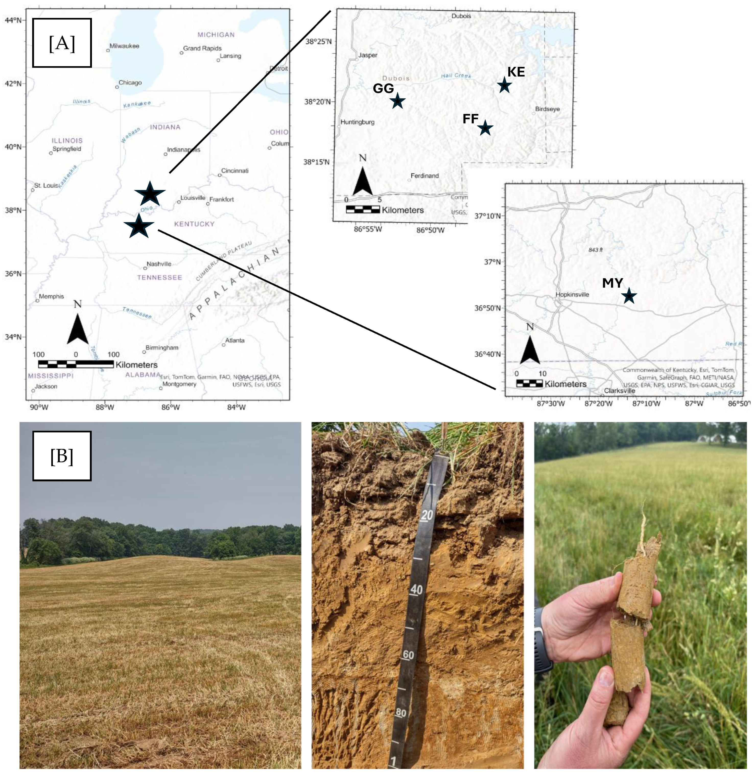
Research locations included 18 fields arrayed across four farms in southern Indiana and western Kentucky (Figure 1). The Indiana farms (FF, GG, and KE) were located in DuBois County near the towns of Maltersville, St. Anthony, and Schnellville with a general location of −87.75° W and 38.31° N. The Kentucky farm (MY) was located in Todd County near −87.25° W and 36.25° N outside of the town of Hopkinsville. This region receives, on average, 1200–1300 mm yr⁻¹ of precipitation with a mean annual temperature of 12.7 to 13.8 °C in Indiana and Kentucky, respectively [35]. The climate in this region lies on the border of the humid continental, hot summers, with year-round precipitation, and humid subtropical climate zones of the Köppen Classification system [36]. These zones are typified by at least one month with a mean temperature below 0 °C, at least one month with a mean temperature >22 °C, at least four months averaging >10 °C, and limited seasonal differences in precipitation. The region lies within the warm, temperate, moist forest region of the Holdridge Life Zones [37] and native vegetation includes predominantly secondary growth mixed deciduous hardwood forests that consist of various mixtures of white oak (Quercus alba), red oak (Q. rubra), black oak (Q. veluntia), bitternut hickory (Carya cordiformis), shagbark hickory (C. ovata), along with flowering dogwood (Cornus florida), sassafras (Sassafras spp.), and hop hornbeam (Carpinus spp.) in the understory [38]. A large fraction of the land area in this region is currently used for agriculture.

The Indiana farm sites were located in the Southern Hills and Lowland Region physiographic province in southern Indiana [39] in an area underlain by the Pennsylvanian-aged Raccoon Creek Group that consists mostly of shale and sandstone bedrock, with thin beds of limestone, clay, and coal [40]. These bedrock materials are generally capped with >1 m of Peoria loess, deposited following the Last Glacial Maximum and retreat of the Wisconsin Glaciation, overlying residuum [41,42]. The Kentucky farm site was located in the Pennyroyal Region of western Kentucky near the contact of the Mississippian Plateau and Dripping Springs Escarpment. The bedrock in the region around the farm site was primarily the Mississippian-aged Big Clifty Sandstone Member of the Golconda Formation, comprising siltstone, sandstone, and shale, that is capped with deposits of Peoria loess of variable thickness [43,44].

Soils on the Indiana farm sites primarily consisted of the Zanesville soil series (fine-silty, mixed, active, mesic Oxyaquic Fragiudalf), with small areas of the Apalona (fine-silty, mixed, active, mesic Oxaquic Fragiudalf), and Gilpin (fine-loamy, mixed, active, mesic Typic Hapludult) soil series [45]. The Apalona and Zanesville series both exhibit ~1 m of loess cover over weathered residuum, with variable expression of a fragipan at depths of ~65–100 cm below the soil surface. The Gilpin series is limited to eroded slopes with little to no loess cover and is primarily derived from weathered bedrock. All soil cores collected on the Indiana farms exhibited the loess over weathered bedrock stratigraphy typical of the Zanesville soil series (Figure 1). Soils on the Kentucky farm site primarily included the Zanesville soil series, along with small areas mapped as the Frondorf (fine-loamy, mixed, active, mesic Ultic Hapludalf), and the Nicholson (fine-silty, mixed, active, mesic Oxyaquic Fragiudalfs) soil series [45]. The Nicholson series generally has ~1 m of loess cover over bedrock with a weak fragipan at depths of ~60–100 cm, and the Frondorf series generally exhibits ~0.5 m thick loess cover over weathered bedrock and lacks the fragipan. All soil cores collected on the Kentucky farm exhibited the loess over weathered bedrock stratigraphy typical of the Zanesville and Nicholson soil series.

2.2. Sampling Design

The sampling design was oriented around replicated sampling of five different management systems. The management systems included (1) conventional corn with annual tillage (CONV); (2) conventionally managed fields that were converted to an ICLS nearly two decades prior to sampling (ICLS-15); (3) conventionally managed fields that were converted to ICLS 4–5 years prior to sampling (ICLS-5); (4) multidecadal fescue pasture with varying degrees of rotational grazing (PAST); and (5) native deciduous hardwood forest (WOOD). Sampling of the Indiana farms occurred in the summer and fall of 2023, while sampling at the Kentucky farm occurred in summer 2024.

The CONV system involves corn production for grain, with planting typically occurring around 1 May and harvest in early October. Tillage is performed at planting to prepare the seedbed. Nitrogen fertilization includes a moderate application of 50–55 kg N ha⁻¹ in late May, followed by a heavier application of 135–170 kg N ha⁻¹ in late June to support crop growth during the peak growing season.

The ICLS treatments feature a no-till, drill-seeded rotation of either corn silage/annual ryegrass or corn silage/winter wheat. Herbicide is applied between crop transitions (post-harvest and pre-planting). Winter forage crops (wheat or annual ryegrass) are typically grazed from around 1 November to 15 December at a stocking rate of 1 head per 0.6–0.8 ha with 40% forage utilization. Corn silage is typically planted around 30 May and harvested around 15 September, following a manure application of 14.5 tonnes ha⁻¹ in late May. Nitrogen is applied at approximately 50 kg N ha⁻¹ at planting and 160 kg N ha⁻¹ during peak growth in late June. Winter wheat, used for both grazing and silage, is planted in early October and harvested in mid-May. It receives 14.5 tonnes ha⁻¹ of manure in September (post-corn harvest), ~45 kg N ha⁻¹ after planting, and ~65 kg N ha⁻¹ in mid-March. Similarly, Winterhawk annual ryegrass is planted around 20 September and harvested mid-May, with 14.5 tonnes ha⁻¹ of manure applied post-corn harvest and ~65 kg N ha⁻¹ applied in mid-March during the peak growth period. The ryegrass is inter-seeded with small percentages of wheat and oats to improve forage architecture and reduce matting.

The PAST treatments consist of a fescue-legume mix that varies from resting in winter and spring with grazing from May to December, to resting in summer with grazing from November to April. The pastures are grazed at a stocking rate of one head per 0.6–0.8 ha with 40% utilization in a pattern of 1 week on and 3 weeks off. The summer-rested fields receive annual fertilization at a rate of ~55 kg ha⁻¹. The WOOD treatment consists of mature native hardwood forest sites located adjacent to actively managed fields that exhibited no evidence of recent logging but likely represent secondary growth forests.

Individual fields were treated as blocks of a specific management system. We collected two to six replicate cores from each field to a depth of 120 cm using a truck-mounted Giddings probe (Giddings Machine Company, Windsor, CO, USA, https://www.soilsample.com/; verified 15 May 2025) in cooperation with local Indiana and Kentucky USDA Natural Resources Conservation Service soil scientists. We aimed for 5 core locations per field, distributed randomly across the field within certain topographic constraints. Core locations were determined using a random stratified field design that accounted for field-scale variation in slope and drainage. Specifically, core locations were limited to landscape positions where the slope was less than 10% and to areas with convex or linear curvature to minimize the effects of erosion and deposition on SOC content. Topographic data were extracted from Lidar-derived digital elevation model data available from the Indiana Statewide Imagery and Lidar program (IndianaMap, 2011, https://www.indianamap.org/; verified 15 May 2025) for the Indiana-based farms at 1.5 m resolution, and from USGS 10 m resolution digital elevation models for the Kentucky farms. Slope and curvature were calculated for each farm using ArcGIS Pro v3.1.2 (ESRI, Redlands, CA, USA). The percent slope maps were reclassified to identify areas with slopes of ≤10% and converted from a raster format to vector-based polygons. The ≤10% slope polygons were dissolved into one polygon and clipped to the boundary of each field. The field boundaries included a 10 m internal buffer to avoid locating sites in areas with potential edge effects. Some fields had fewer than 5 core samples due to a lack of area that matched the topographic constraints. Core locations were determined for each clipped slope layer using the Sampling Design Tool for ArcGIS developed by the US National Oceanic and Atmospheric Administration (https://coastalscience.noaa.gov/project/sampling-design-tool-arcgis/; verified 15 May 2025). The design maintained at least a 25 m separation among sample locations. Core locations were reviewed with the local landowners prior to sampling to ensure we avoided areas with spurious management histories, such as past manure or silage stockpiles. In the few instances where site locations required adjustment, we moved locations to adjacent low-sloping areas on similar landforms.

Soil cores were collected into clear 4.5 cm diameter PETG tubes to a depth of 120 cm using the Giddings probe. The cores were capped, labeled, and cut into three depths onsite at depth intervals of 0–30 cm, 30–60 cm, and 60–120 cm following GraceNet protocols [46] at the time of sampling. Cores were stored in coolers until returned to the laboratory, where they were stored at 5 °C in a refrigerator until processed for physical and chemical analyses.

2.3. Soil Analyses

2.3.1. Bulk Density and Porosity

Bulk density was determined for each core section. The entire core section was weighed after returning from the field to obtain wet soil weight, correcting for the mass of the tube and end caps. A 30 to 60 g subsample of field-moist soil material was collected from each core section, oven-dried at 105 °C, and re-weighed multiple times until the same mass did not change to determine the oven-dry mass and water content at field conditions. The core section water content was used to correct the mass of the entire core section and determine a total core section oven-dry soil mass. Bulk density was then calculated using the total core section oven-dry soil mass and core section volume [47].

Porosity ($\varnothing$) was calculated from bulk density

$$\varnothing =1-{\rho }_b/{\rho }_p,$$

(1)

where ${\rho }_b$ is oven-dry soil bulk density (kg m⁻³) calculated from the core samples, ${\rho }_p$ is assumed fixed at 2650 kg m⁻³, and porosity values are reported as a decimal fraction [48].

2.3.2. Soil Carbon Content

Each core section was subsampled for soil physical and chemical characterization. After weighing the core sections for bulk density analysis, the sections were cut in half down the long axis using a knife. Half of the core section was collected for physicochemical analyses and determining water content, and the other half was air-dried and archived.

Subsamples from all core sections were analyzed at Brookside Laboratories (https://www.blinc.com/, New Bremen, OH, USA; verified 15 May 2025) for a suite of soil physicochemical properties, including total C by combustion [49]. None of the soils contained inorganic C based on the observation of strongly acidic pH values and a lack of reactivity with acid, such that total C measured by combustion was assumed equivalent to total organic C. Approximately one quarter of the samples returned total C values less than the Brookside Laboratories detection limit of 0.2%. All of the samples were from the deep core sections collected between 60 and 120 cm. The below detection limit samples, and a selected subset of reference surface samples, were subsampled and analyzed at the Oklahoma State University (OSU) Soil, Water and Forage Analytical Laboratory (https://agriculture.okstate.edu/departments-programs/plant-soil/soil-testing/, Stillwater, OK, USA; verified 15 May 2025) for total combustible C. The OSU lab reports a detection limit of 0.05% organic C, and all values measured on the core sections were greater than 0.08%. The reference samples from both labs had comparable results, and the values obtained from the OSU lab for the deep core sections were integrated into the dataset.

Soil C data were reported as weight percent (SOC, %), converted to a SOC density (SOC_DENS, kg m⁻³):

$${SOC}_{DENS}=C·{\rho }_b,$$

(2)

where C is the decimal percent SOC (kg C kg⁻¹), and ${\rho }_b$ is oven dry bulk density (kg m⁻³); note that a rock fragment volume correction was not included as no rock fragments were observed in the core samples. SOC was further converted to a SOC stock (SOC_STOCK, Mg ha⁻¹) summed over the entire profile:

$${SOC}_{STOCK}={\displaystyle {\sum }_{i=1}^n}{SOC}_{DENSi}·h_i·10,$$

(3)

where n is the total number of depth increments i, SOC_DENS is the SOC density (kg m⁻³), h_i is the thickness of each depth increment (m), and 10 is a conversion factor from kg m⁻² to Mg ha⁻¹. The SOC stock values were also reported on a CO₂ equivalent basis (CO_2e, tonnes CO₂ acre⁻¹) for comparison with biogeochemical model simulation output:

$${CO}_{2e}={SOC}_{STOCK}·0.405·3.67,$$

(4)

where SOC_STOCK is multiplied by 0.405 to convert from Mg ha⁻¹ to metric tons (tonnes) acre⁻¹, and 3.67 is the ratio of the molecular weights of CO₂ (44 g mol⁻¹) and C (12 g mol⁻¹) [50].

2.3.3. Particulate and Mineral Associated Organic Matter

Three cores were randomly selected from each field, representing all treatments, and soil from each depth increment was analyzed for particulate organic matter (POM) and mineral-associated organic matter (MAOM) mass fractions and C content at Cquester Labs (https://www.cquesteranalytics.com/; verified 15 May 2025) based on particle size following methods outlined by Cotrufo et al. [51], Leuthold et al. [52], and Leuthold et al. [53]. Briefly, bulk soils were dispersed in 0.5% sodium hexametaphosphate, followed by wet-sieving at 53 µm, with POM > 53 µm and MAOM < 53 µm. The bulk soil, POM, and MAOM fractions were analyzed on an elemental analyzer for total C and reported as POM-C (%) and MAOM-C (%). The mass of each fraction as a percentage of the bulk soil, as well as the concentration of C in each fraction, was reported.

The surface soil MAOM and POM fractions were further analyzed for their stable C isotope content (δ¹³C) at the Indiana University Stable Isotope Research Facility using an elemental analyzer coupled to an isotope ratio mass spectrometer (https://earth.indiana.edu/research/research-labs-and-centers/sirf-lab/facilities.html; verified 15 May 2025). Data were reported on a per mil basis (‰) relative to the Vienna Pee Dee Belemnite reference [54].

2.4. Statistical Analyses

Summary statistics were calculated for all soil data to evaluate data distributions, variability, and to check for outliers. One core was excluded from the ICLS-15 samples based on anomalously high SOC well outside 1.5 times the interquartile range of a box and whisker plot. Prior to statistical analyses, all data were transformed individually using a Box–Cox transformation to approximate normal distributions [55]. The soil data were analyzed using linear mixed-effects models to identify and quantify significant differences among the six sampled treatments. Each treatment included two to five fields, treated as blocks, with two to six replicate cores per field. The mixed-effects models included “treatment” as the fixed effect and “Field ID” as the random effect to account for any influence of field-specific variation. The models were performed separately for each depth increment, recognizing the non-independent nature of samples collected from different depths of the same core. The conditional residuals of the mixed-effects models were evaluated to ensure normality and check for heteroskedasticity, and means were compared across treatments using a Tukey HSD post hoc test with an α = 0.05 [56].

Using a space-for-time approach and assuming the CONV treatments represent a reasonable time-zero reference SOC stock for the ICLS treatments, we used a simple linear regression approach to calculate the potential rate of change in SOC stocks following conversion from CONV to ICLS using least square means regression with total SOC stock as the dependent variable and time since conversion (years) as the independent variable. We also fit a piecewise regression, splitting the data into three groups of ~5-year intervals to capture the relative change in accumulation rate over time [23].

2.5. Biogeochemical Modeling

Biogeochemical model simulations were conducted for specific fields to further evaluate the SOC dynamics of the ICLS management practice. The well-established daily time-step version of the CENTURY model [57], termed DAYCENT [58,59,60] was used to simulate plant–soil processes via implementation in the USDA’s COMET-Farm online tool Version 4.0 (https://comet-farm.com/home; verified 15 May 2025). For details on COMET-Farm and how it implements DAYCENT and the USDA’s methods for cropland and grazing system calculations [61,62], the reader is referred to the manual (https://comet-farm.com/COMET-Farm_Manual.pdf; verified 15 May 2025). Historical management and detailed cropland and grazing practices were parameterized for each field to simulate the evolution of SOC stocks under CONV and ICLS management (Table S1).

Model initialization of SOC followed three sequential simulations. A steady-state simulation representing pre-settlement conditions defined equilibrium soil, vegetation, and climate parameters for each site. Historical period simulations (1800s–2000) applied representative management practices derived from standardized historical scenarios to capture major land-use transitions. Recent history simulations (2000 to the initial year of interest) incorporated site-specific management details, including crop sequences, tillage, fertilizer applications, irrigation, and grazing. These simulations collectively established a realistic baseline for SOC, accounting for the cumulative effects of historical land use and management.

During the historical period simulations, management prior to 1980 was parameterized as non-irrigated upland croplands for all fields within the CONV, ICLS-15, ICLS-5, and PAST systems, except for three fields (FF-HENE, FF-SDW, and FF-WE), which were represented as non-irrigated livestock grazing parcels. No parcels were enrolled in the US Department of Agriculture Conservation Reserve Program during this period. From 1980 to 2000, all fields were modeled as non-irrigated cropland under annual crop rotations with reduced tillage, except FF-HENE was assigned intensive tillage, and the PAST fields (FF-SDW, FF-WE, and FF-WS) were maintained as non-irrigated livestock grazing systems.

Management patterns reflected the system type. ICLS fields (both ICLS-15 and ICLS-5) were characterized by diverse rotations. In the early 2000s, these fields primarily produced corn grain (≈150 bu acre⁻¹) and wheat (≈70 bu acre⁻¹). Beginning in 2011, management shifted toward corn silage (≈20 tons acre⁻¹) integrated with annual ryegrass cover crops (≈3–5 tons acre⁻¹), marking a transition from grain-dominated rotations to silage-plus-cover systems. CONV fields maintained continuous corn systems without cover crops, serving as the grain-only control. PAST fields remained in perennial grassland, producing modest but stable forage yields (≈2–4 tons acre⁻¹) and providing continuous cover with minimal disturbance.

3. Results

3.1. Soil Physical Properties

All the sampled soils were formed in Peoria loess and primarily mapped as the Zanesville soil series, which consists of Fragiudults with weakly developed fragipans that have upper boundaries at depths ranging from 60 to 100 cm below the soil surface. Soil textures exhibited little variation among treatments, or with depth, and were primarily silt loams and silty clay loams with average clay, silt, and sand contents of 27 ± 5.5%, 59 ± 10%, and 14 ± 9.8%, respectively. Silt and sand contents exhibited the largest range and variability across all sites in the 60–120 cm depth, associated with variable depth to fragipan and the lithologic discontinuity between loess and residuum soil of weathered bedrock.

Bulk density values generally increased with depth from an average of 1.24 ± 0.12 g cm⁻³ in the upper 0–30 cm across all treatments, to 1.33 ± 0.09 g cm⁻³ in the 30–60 cm depth, and to 1.47 ± 0.10 g cm⁻³ in the 60–120 cm depths. The upper depth intervals exhibited significant variation among treatments, with the largest differences noted in the 0–30 cm depth interval, where bulk density was lowest in WOOD with average values of 1.02 ± 0.03 g cm⁻³ and the highest value of 1.32 ± 0.02 in CONV treatments (

Table 1. Soil physical and organic carbon data by depth increment for each treatment. Organic carbon data include percent soil organic carbon (SOC), soil organic carbon density (SOC_DENS), and CO₂ equivalence (CO_2e). Values represent means followed by standard error. Means followed by different letters indicate significant differences among treatments withing a given depth interval based on analysis by a linear mixed-effects model with post hoc Tukey HSD means comparison (α = 0.05).

Treatment	Depth	n	Bulk Density	Porosity	SOC	SOCDENS	CO2e
	(cm)		(g cm−3)	(cm3 cm−3)	(%)	(kg m−3)	(tonnes acre−1)
WOOD	0–30	10	1.02 ± 0.03 C	0.61 ± 0.01 A	1.21 ± 0.08 AB	12.31 ± 0.80 AB	55.3 ± 3.60 AB
PAST	0–30	11	1.20 ± 0.02 B	0.55 ± 0.01 B	1.36 ± 0.10 A	16.34 ± 1.21 AB	73.4 ± 5.43 AB
CONV	0–30	30	1.32 ± 0.02 A	0.50 ± 0.01 C	0.88 ± 0.05 B	11.55 ± 0.58 B	51.9 ± 2.58 B
ICLS-5	0–30	11	1.23 ± 0.03 B	0.54 ± 0.01 B	1.11 ± 0.08 AB	13.66 ± 1.0 AB	61.4 ± 4.48 AB
ICLS-15	0–30	18	1.25 ± 0.02 B	0.53 ± 0.01 B	1.42 ± 0.08 A	17.61 ± 0.86 A	79.1 ± 3.84 A
WOOD	30–60	10	1.22 ± 0.03 B	0.54 ± 0.01 A	0.48 ± 0.04 A	5.80 ± 0.42 A	26.0 ± 1.89 A
PAST	30–60	11	1.34 ± 0.01 AB	0.50 ± 0.0 AB	0.32 ± 0.02 B	4.28 ± 0.19 AB	19.2 ± 0.84 AB
CONV	30–60	30	1.40 ± 0.02 A	0.47 ± 0.01 B	0.29 ± 0.01 B	4.02 ± 0.17 B	18.0 ± 0.78 B
ICLS-5	30–60	11	1.30 ± 0.02 AB	0.51 ± 0.01 AB	0.32 ± 0.02 B	4.11 ± 0.20 B	18.5 ± 0.92 B
ICLS-15	30–60	18	1.32 ± 0.01 AB	0.50 ± 0.0 AB	0.33 ± 0.04 B	4.25 ± 0.48 B	19.1 ± 2.15 B
WOOD	60–120	10	1.40 ± 0.03 A	0.47 ± 0.01 A	0.28 ± 0.03 A	3.96 ± 0.36 A	35.6 ± 3.22 A
PAST	60–120	11	1.46 ± 0.03 A	0.45 ± 0.01 A	0.24 ± 0.01 A	3.55 ± 0.11 A	31.9 ± 1.01 A
CONV	60–120	30	1.50 ± 0.02 A	0.43 ± 0.01 A	0.20 ± 0.01 A	2.89 ± 0.2 A	25.9 ± 1.75 A
ICLS-5	60–120	11	1.47 ± 0.02 A	0.44 ± 0.01 A	0.23 ± 0.01 A	3.32 ± 0.10 A	29.8 ± 0.88 A
ICLS-15	60–120	18	1.49 ± 0.02 A	0.44 ± 0.01 A	0.25 ± 0.01 A	3.68 ± 0.17 A	33.1 ± 1.55 A

). The other PAST and ICLS treatments ranged between 1.20 and 1.23 g cm⁻³ with no significant differences among them. The CONV treatment was also significantly greater than WOOD in the 30–60 cm depth interval. Porosity values were greatest in WOOD across all depths (Table 1). Values were significantly greater than all treatments in the 0–30 cm depth interval and significantly greater than CONV in the 30–60 cm depth interval, with PAST and both ICLS treatments exhibiting intermediate values. CONV treatments exhibited porosity values significantly less than all other treatments in the surface horizon (Table 1).

3.2. Soil Organic Carbon Concentration and Stocks

SOC concentrations decreased substantially with depth across all treatments, with surface concentrations averaging 1.14 ± 0.35% and 14.0 ± 4.0 kg m⁻³ in the 0–30 cm depth interval and declining to 0.23 ± 0.06% and 3.39 ± 0.9 kg m⁻³ in the 60–120 depth interval (Table 1). Significant differences among treatments were observed in 0–30 cm and 30–60 cm depth intervals. In the upper 30 cm, the SOC % in the PAST and ICLS-15 treatments were significantly greater than CONV; all other treatments were intermediate. SOC_DENS values were significantly greater in ICLS-15 relative to CONV. The only significant difference observed in the 30–60 cm depth interval was greater SOC % in WOOD relative to all the other treatments. These differences were also present in the SOC_DENS data, except that the PAST treatment expressed intermediate values relative to WOOD and the other treatments. No significant differences were observed in the 60–120 cm depth interval.

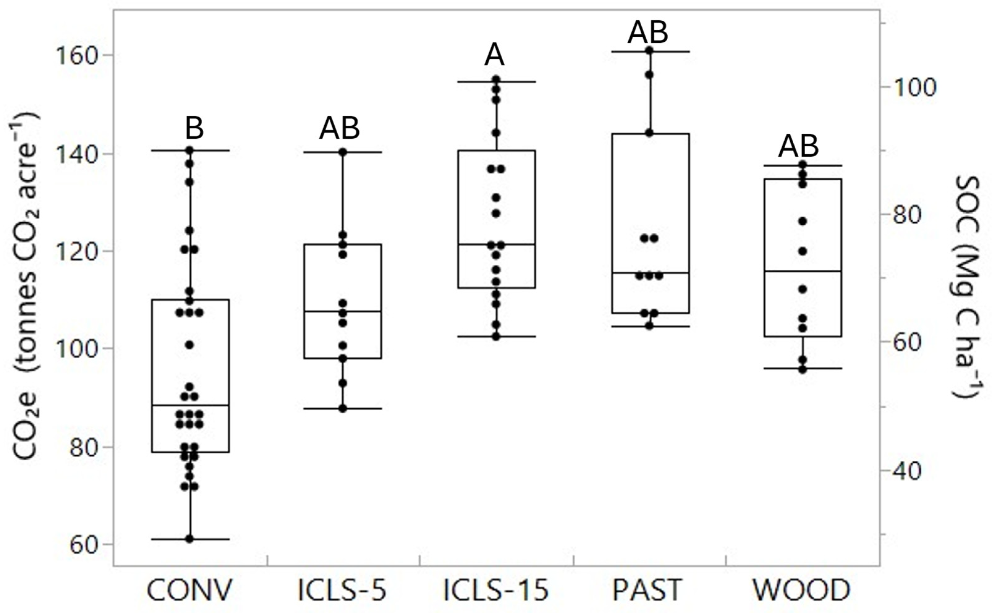
The SOC_STOCK values showed significant differences among treatments (Figure 2). The greatest SOC_STOCK was observed in the ICLS-15 treatment with 85.3 ± 2.80 Mg ha⁻¹, equivalent to 127 ± 4.1 tonnes CO₂ acre⁻¹, which was significantly greater than CONV (p = 0.0196) that averaged only 64.5 ± 2.6 Mg ha⁻¹, or 95.9 ± 3.9 tonnes CO₂ acre⁻¹. All other treatments were intermediate between these two values.

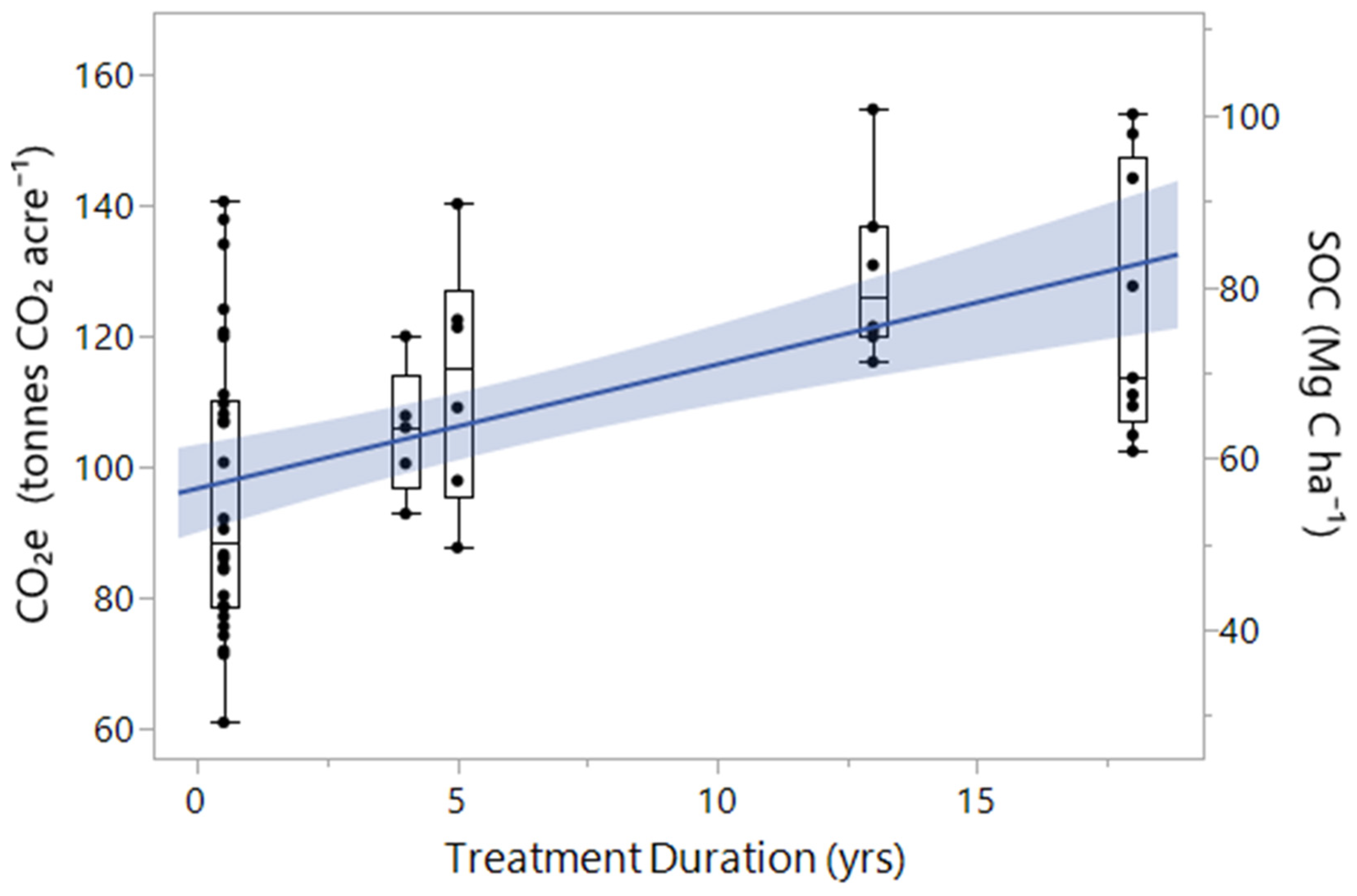
The rate of change in SOC_STOCK with conversion of CONV to ICLS was modeled using a space-for-time approach where the CONV treatments were assumed to represent baseline SOC stocks at time zero, and the duration each field has been managed with ICLS was used as treatment time (Figure 3). Linear regression analysis across the entire time series demonstrated a significant SOC increase over time, with a modeled annual rate of gain of 1.3 Mg C ha⁻¹ year⁻¹ (0.8–1.8 Mg C ha⁻¹ year⁻¹, 95% confidence interval), equivalent to 1.9 tonnes CO₂ acre⁻¹ year⁻¹ (1.1–2.6 tonnes CO₂ acre⁻¹ year⁻¹, 95% confidence interval). Fitting piecewise rates between each time interval yielded a change in rate from 2.3 Mg C ha⁻¹ yr⁻¹ during the years 0–5, to 1.6 Mg C ha⁻¹ yr⁻¹ in years 5–13, to near zero change rate after year 13.

3.3. Soil Organic Carbon Partitioning to Mineral and Particulate Fractions

All horizons were dominated by MAOM as a percentage of the total soil mass, with MAOM comprising 75–95% of the total (

Table 2. Mineral-associated organic matter (MAOM) and particulate organic matter (POM) values for each treatment and depth interval. Values include the total mass fraction, percent organic carbon, and percentage of total organic carbon for both MAOM and POM fractions. Values represent means followed by standard error. Means followed by different letters indicate significant differences among treatments within a given depth interval based on analysis by a linear mixed-effects model with post hoc Tukey HSD means comparison (α = 0.05).

Treatment	Depth	n	MAOM	MAOM-C	MAOM-C	POM	POM-C	POM-C
	(cm)		(% of Total Mass)	(%)	(% of Total C)	(% of Total Mass)	(%)	(% of Total C)
WOOD	0–30	10	95.9 ± 2.65 A	0.84 ± 0.08 A	77.7 ± 1.89 B	5.36 ± 2.60 A	5.70 ± 1.07 A	22.3 ± 1.89 A
PAST	0–30	11	91.8 ± 6.0 A	0.90 ± 0.10 A	80.9 ± 1.67 AB	8.98 ± 6.16 A	2.86 ± 0.47 A	19.1 ± 1.67 AB
CONV	0–30	24	93.8 ± 4.01 A	0.55 ± 0.04 A	86.4 ± 0.96 A	6.78 ± 3.50 A	1.70 ± 0.28 A	13.6 ± 0.96 B
ICLS-5	0–30	6	96.7 ± 1.27 A	0.86 ± 0.08 A	80.8 ± 2.81 AB	4.37 ± 1.22 A	4.76 ± 0.99 A	19.2 ± 2.81 AB
ICLS-15	0–30	10	92.6 ± 3.91 A	0.86 ± 0.06 A	76.9 ± 2.28 B	8.19 ± 4.04 A	3.34 ± 0.51 A	23.1 ± 2.28 A
WOOD	30–60	10	97.2 ± 3.40 A	0.20 ± 0.01 A	91.5 ± 1.48 A	3.85 ± 3.54 A	0.89 ± 0.22 A	8.51 ± 1.48 A
PAST	30–60	11	92.6 ± 7.70 A	0.18 ± 0.02 A	95.5 ± 1.16 A	7.82 ± 7.81 A	0.17 ± 0.07 A	4.47 ± 1.16 A
CONV	30–60	24	92.2 ± 9.42 A	0.11 ± 0.01 A	91.9 ± 1.87 A	8.53 ± 9.34 A	0.24 ± 0.07 A	8.11 ± 1.87 A
ICLS-5	30–60	6	97.5 ± 3.02 A	0.17 ± 0.02 A	92.6 ± 0.92 A	3.42 ± 3.05 A	0.69 ± 0.20 A	7.45 ± 0.92 A
ICLS-15	30–60	10	94.9 ± 3.27 A	0.20 ± 0.07 A	90.5 ± 1.36 A	5.61 ± 3.22 A	0.44 ± 0.14 A	9.46 ± 1.36 A
WOOD	60–120	10	87.9 ± 9.19 A	0.09 ± 0.01 A	81.8 ± 4.91 A	12.6 ± 9.41 A	0.26 ± 0.11 A	18.2 ± 4.91 A
PAST	60–120	11	74.5 ± 12.1 A	0.08 ± 0.01 A	89.9 ± 1.33 A	25.9 ± 12.2 A	0.03 ± 0.01 B	10.2 ± 1.33 AB
CONV	60–120	24	81.6 ± 12.8 A	0.09 ± 0.02 A	89.8 ± 1.85 A	18.6 ± 12.6 A	0.10 ± 0.06 B	10.2 ± 1.85 AB
ICLS-5	60–120	6	76.5 ± 8.09 A	0.05 ± 0.01 A	87.1 ± 2.12 A	24.2 ± 8.21 A	0.02 ± 0.0 B	12.9 ± 2.12 AB
ICLS-15	60–120	10	86.6 ± 6.96 A	0.08 ± 0.02 A	95.6 ± 1.44 A	13.6 ± 7.08 A	0.02 ± 0.01 B	4.39 ± 1.44 B

). The concentration of MAOM-C averaged 0.33 ± 0.03% across all horizons, with a trend of decreasing concentration with depth, where surface horizons averaged 0.74 ± 0.03% and declined to an average of 0.08 ± 0.01% in the 60–120 cm depth interval. MAOM-C as a percentage of total SOC tended to increase with depth, averaging 76.9 ± 1.1% in the upper 0–30 cm depth interval and increasing to 93.4 ± 1.7% in the lower horizons.

Particulate organic matter as a percentage of the total soil mass averaged 6.9 ± 0.5% in the upper 0–30 cm and increased to 18.7 ± 11.6% in the 60–120 cm depth interval (Table 2). The increase in total mass of POM is strongly correlated with increasing sand content in the deep horizons (r² = 0.80, p < 0.0001). The concentration of POM-C decreased substantially with increasing depth, with average values of 3.1 ± 0.3% in the upper horizon decreasing to an average of 0.1 ± 0.03% in the deepest horizons. POM-C as a percentage of total SOC also tended to decrease with depth, transitioning from an average of 17.1 ± 0.9% in the 0–30 cm depth interval to an average of 12.6 ± 1.4% in the 60–120 cm depth interval.

There were relatively few significant differences in MAOM and POM parameters by depth interval across treatments (Table 2). The only significant differences were observed in the relative distribution of total SOC to MAOM and POM in the 0–30 cm depth interval, where CONV exhibited significantly greater MAOM-C as a percent of the total than the WOOD (p = 0.0201) and ICLS-15 treatments (p = 0.0133) (Table 2). The POM-C as a percent of total C was also significantly different among these treatments, with significantly less POM-C as a percent of the total in the CONV treatment relative to WOOD (p = 0.0227) and ICLS-15 (p = 0.0168). There was a trend of a lower concentration of C in MAOM fractions in the CONV treatment, with average values of 0.55% relative to the other treatments, where averages ranged from 0.84 to 0.90%. Several of these differences bordered on significance, with pairwise comparison p-values of p = 0.0567 comparing CONV and PAST, and p = 0.0885 comparing CONV and ICLS-15. The only other significant differences among treatments were observed in the 60–120 cm depth interval, where the POM-C as a fraction of total C was significantly greater in the WOOD relative to ICLS-15 (p = 0.002) (Table 2).

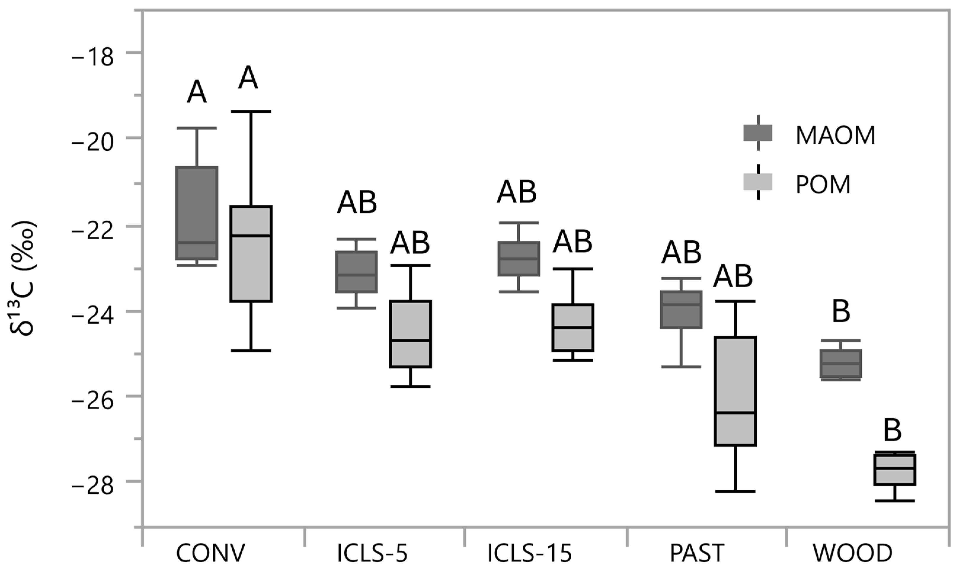
Surface horizon MAOM and POM stable isotope data indicated significant variation in the contribution of different carbon sources across treatments among each fraction (Figure 4). The CONV treatment MAOM and POM fractions were significantly enriched in ¹³C relative to the WOOD fractions (p = 0.0239 and p = 0.0178, respectively). There was a trend of more depleted ¹³C values in the ICLS and PAST treatments relative to CONV, but differences were not significant. The relatively enriched values of ¹³C in the CONV fractions indicated a greater contribution of C4-derived carbon to MAOM and POM fractions relative to the other treatments. All treatments also exhibited ~0.5 to 2 per mil enrichment in MAOM-C relative to POM-C, typical of enrichment associated with microbial degradation [63].

3.4. Biogeochemical Modeling Results

Simulated soil carbon stock change (tonnes CO₂ acre⁻¹ yr⁻¹) in the top 30 cm of soil revealed distinct differences among management systems, with negative values indicating carbon sequestration and positive values representing carbon loss. CONV fields were effectively carbon-neutral but trended slightly toward depletion, showing minor losses ranging from +0.01 to +0.40 tonnes CO₂ acre⁻¹ yr⁻¹, with an average of +0.15 ± 0.10. In contrast, ICLS fields showed consistent SOC gains. The ICLS-15 fields sequestered −2.86 to −1.93 tonnes CO₂ acre⁻¹ yr⁻¹, with an average of −2.45 ± 0.23, while the ICLS-5 fields exhibited the highest and most variable sequestration, ranging from −7.15 to −1.42 tonnes CO₂ acre⁻¹ yr⁻¹, with an average of −2.31 ± 1.59.

PAST fields also acted as carbon sinks, with moderate sequestration ranging from −1.88 to 0.0 tonnes CO₂ acre⁻¹ yr⁻¹. Literature values for similar rotational grazing systems [64] estimated a sequestration rate of −0.4 Mg C ha⁻¹ yr⁻¹, equivalent to −0.30 tonnes CO₂ acre⁻¹ yr⁻¹ in the top 100 cm of soil, somewhat lower than the DAYCENT projections calculated in this study. Overall, the biogeochemical model indicated CONV systems showed slight SOC losses, whereas ICLS and PAST systems achieved net sequestration, with the ICLS-5 fields exhibiting the highest, but most variable, SOC gains.

4. Discussion

There was substantial variation in total SOC stocks among the different systems (Figure 2). The greatest SOC stocks were observed in the ICLS-15 treatments with an average stock of 85.3 ± 2.8 Mg ha⁻¹ that was significantly greater than the CONV stock of 64.5 ± 2.6 Mg ha⁻¹. The PAST and WOOD treatments also had SOC stocks >75 Mg ha⁻¹, whereas the ICLS-5 treatment averaged 73.8 ± 3.1 Mg ha⁻¹. These values are comparable to, and somewhat higher than, average SOC stocks calculated for midwestern USA states and southern Indiana from soil survey data that averaged on the order of 50 Mg ha⁻¹ [65,66,67]. Nave et al. [68] also calculated SOC stocks on the order of ~50 Mg ha⁻¹ for mixed mesophytic, oak-hickory, oak-pine, and pine-dominated forests with similar temperature and precipitation of the south Atlantic seaboard in southeastern USA forests. The data indicated that long-term pasture management maintained relatively high SOC stocks that were comparable to and slightly greater than those of native hardwood forest, in agreement with previous assessments of SOC stock change with conversion of forest to pasture [69]. Comparing the CONV and WOOD treatments indicated that long-term conventional management resulted in a ~30% loss of SOC relative to native hardwood forests. This loss is comparable to other studies, noting up to 25–42% loss of SOC with the conversion of forest to conventionally managed agriculture [2,4,19,25,69].

A key finding from this study was that the conversion to integrated crop–livestock system management increased SOC stocks to levels equivalent to, and slightly greater than, the native hardwood forest (Figure 2). This increase is greater than the 7–17% increase in SOC measured in meta-analyses comparing conventional with no-till and annual cover crop rotation management across a wide range of geographic and management systems [18,19], but comparable to the ~15–30% increase determined in the meta-analysis of Joshi et al. [20] that largely focused on soils from the Midwestern USA. The greatest SOC gains across all the meta-analyses were consistently observed in the most degraded soils that had SOC < 1% and in temperate climate systems with mean annual temperatures < 15 °C. The meta-analyses found a somewhat variable influence of soil texture on the relative SOC gain with cover crops, with Joshi et al. [20] observing the largest changes in fine-textured soils, whereas Blanco-Canqui [18] and Jian et al. [19] found relatively minimal influence of texture on SOC change, with a trend of slightly less SOC change in fine-textured soils. The conventional fields sampled in this study exhibited SOC concentrations that averaged <1%, all the field sites were in temperate climates with mean annual temperatures < 15 °C, and soil textures were predominantly medium and fine-textured silt loams and silty clay loams. The fields thus exhibited very favorable conditions and capacity for increased SOC storage that likely explain the relatively large observed gains in SOC.

Studies documenting SOC change with conversion to ICLS in the Midwestern USA also indicate a substantial increase in surface SOC content. For example, Tracy and Zhang [29] measured ~17% increase in SOC in the 0–15 cm depth three years after conversion from conventional continuous corn to an ICLS that consisted of an oat or corn summer cash crop in rotation with a winter cover crop mixture of oat, cereal rye, and turnip used for grazing at a study site in central Illinois, USA. By year five, the same study sited showed a ~55% increase in SOC concentration in the upper 20 cm relative to conventional corn [34]. In comparison, Dhaliwal and Kumar [1] observed SOC gains of 20–26% in the upper 5 cm of a long-term (>30 yr) ICLS experiment that included incorporation of cover crops and livestock grazing into existing corn-soybean cropping systems in South Dakota.

The varying time of ICLS management across the sites sampled in this study allowed for calculating an average rate of change in SOC stocks up to 18 years following conversion to ICLS, assuming the measured CONV SOC stocks represent a reasonable time-zero reference (Figure 3). The average rate of change was 1.3 Mg C ha⁻¹ yr⁻¹ (0.8–1.8 Mg C ha⁻¹ yr⁻¹, 95% confidence interval), equivalent to 1.9 tonnes CO₂ acre⁻¹ yr⁻¹ (1.0–2.6 tonnes CO₂ acre⁻¹ yr⁻¹, 95% confidence interval). Fitting piecewise rates between each time interval yields a change in rate from 2.3 Mg C ha⁻¹ yr⁻¹ during the years 0–5, to 1.6 Mg C ha⁻¹ yr⁻¹ in years 5–13, to a near-zero rate of change after year 13. These rates are similar in pattern and magnitude to those simulated using COMET-Farm. This pattern suggests that SOC approached a new steady-state after about a decade of ICLS management [70], likely near the limit of potential SOC gain and similar to the carbon saturation concept of West and Six [23]. There is relatively limited data on rates of SOC stock accrual in Midwestern US integrated crop livestock systems, but these rates are in line with the higher end of rates in the data synthesis of Villat and Nicholas [71] that reported ICLS SOC accrual rates of ~0.4 to 1.5 Mg C ha⁻¹ yr⁻¹ across a range of systems. Results are also consistent with data from an Oxisol in Brazil with an ICLS consisting of summer soybean production and continuous grazing of winter Italian ryegrass that showed rates of ~1.6 Mg C ha⁻¹ yr⁻¹ during the first seven years [12]. There are more studies in the literature for cover crop and no-till management systems that, in comparison, give average rates of SOC gain of 0.1 to 1.1 Mg C ha⁻¹ yr⁻¹ [9,18,19,20,21,22]. The average value of 1.3 Mg C ha⁻¹ yr⁻¹ observed in the current study aligns well with these studies, though notably at the high end of the reported sequestration rates. It should be noted that there are limitations and drawbacks to a space-for-time approach for the calculation of SOC accrual. The limitations include potential variability in soil properties, either due to spatial heterogeneity or variation in the actual “time-zero” SOC stocks, as well as variation in management history among field sites. We attempted to minimize these limitations by constraining sites to the same soil series and landscape position and coupling empirical measurements of SOC stocks with model simulations that accounted for management history. However, a true site-specific chronosequence with paired sampling would provide a more robust approximation of SOC stock change over time.

The majority of SOC change occurred in the 0–30 cm depth interval, in agreement with previous studies and meta-analyses. The majority of new surface horizon SOC in the ICLS treatments was partitioned to POM-C when quantified as a percentage of total SOC (Table 2). POM-C as a percentage of the total increased from only ~13% in the CONV treatments to over 23% in the ICLS-15 treatment, comparable to values observed in the native forest reference sites. Conversely, the CONV treatments exhibited greater dominance of SOC partitioning to MAOM-C, with >86% of total SOC in MAOM fractions. The POM-C fraction is the SOC fraction most susceptible to change with shifts in soil management and may be considered an early indicator of SOC change [72,73,74]. POM generally represents an accrual of litter and residue, organic amendments, and root inputs and can be used as a short-term indicator of SOC dynamics [75]. This material lacks physical protection by minerals or aggregates and is susceptible to decomposition and rapid change with management [76]. The lack of POM-C in the CONV treatments was likely driven by a relative lack of residue inputs, surface erosion, and rapid decomposition. In contrast, the ICLS that includes no-till and grazing of winter cover crops increased litter residue and root inputs, and minimized erosive losses, allowing for relatively rapid gain in POM-C. The POM fraction is an important source of soil nutrients, serves as an energy source for microorganisms, and can facilitate soil aggregation and maintenance of soil structure. The increase in POM-C in the ICLS thus contributes significant soil health benefits. Carvalho et al. [12] also observed a relatively rapid (<6 yr) increase in POM-C following conversion to ICLS in a soybean/ryegrass rotation with cover crop grazing on a subtropical Oxisol in Brazil. The increase in POM-C accounted for the majority of gains in SOC stocks. In contrast, Cates et al. [72] found a limited increase in POM with the incorporation of bluegrass or ryegrass cover crops into continuous corn grain or corn silage production systems after 3 years of management. However, this study was performed on SOC-rich Mollisols in central Wisconsin, and the lack of significant effect may have been obscured by initially high SOC levels, similar to other studies on cover crops’ effects on SOC gain [18].

While POM-C as a percentage of total SOC increased with conversion to ICLS, we also observed an increased concentration of MAOM-C in the surface horizons of the ICLS treatments, with values nearly double those recorded in CONV treatments (Table 2). MAOM-C generally represents a stable and persistent form of SOC with decadal to centennial time scale turnover times [51]. The observed gains in MAOM-C are thus important for the development of persistent SOC stocks. The MAOM-C and POM-C fractions in the ICLS, PAST, and WOOD treatments expressed a depleted δ¹³C signature relative to the CONV treatments, indicating a greater proportion of C3 plant-derived C (Figure 4). This pattern was expected in the PAST and WOOD treatments that are dominated by C3 plants. The shifts in isotopic signature following conversion of CONV to ICLS occurred rapidly (<5 yr) in both fractions, suggesting dynamic cycling and incorporation of new depleted C into SOC fractions. The ICLS fields receive carbon inputs from ryegrass, corn, and manure, including manure deposited during grazing of the ryegrass and manure collected from feed barns where cattle are fed a mixed diet of C3 and C4 feedstock. The δ¹³C signature of ryegrass typically falls between −33‰ and −25‰, with an average of ~−30‰, whereas corn typically falls between −9‰ and −15‰, with an average of ~−11‰ [77,78]. Any manure deposited during the grazing of ryegrass would reflect the depleted C3 signature of the ryegrass. However, the fields also received manure collected during periods of feeding with corn silage that would reflect the enriched δ¹³C signature of corn. The overall manure δ¹³C signature thus likely represents a mixture of C3 and C4 carbon, given the mixed diet of the cows. If we assume a 50/50 mixture of C3 and C4 carbon with stable isotope ratios of −30‰ and −11‰, the manure would average −20.5‰. The ICLS treatment MAOM and POM δ¹³C values average −23‰ and −25‰, respectively, in comparison with values of −22‰ to −22.5‰ in the CONV treatment. The relatively depleted isotopic signature in the ICLS treatments suggests a bias towards C3 carbon, even with a potentially mixed isotopic signal from manure inputs, suggesting the annual ryegrass cover crop is likely the dominant source of the observed SOC gains.

Overall, the increase in SOC with ICLS management was likely driven by several covarying factors, including the shift to no-till, the incorporation of the annual winter ryegrass cover crop, additional organic amendments, and annual grazing of the winter cover crop. As noted, no-till and inclusion of annual cover crops have been shown to yield up to a 15% increase in SOC relative to conventional management [20], and could explain a substantial portion of the SOC gains recorded in this study. The ICLS study sites also receive annual applications of partially composted manure at rates on the order of 29 tonnes ha⁻¹ yr⁻¹, as well as direct manure inputs during grazing, which likely contribute to increased SOC. Annual ryegrass has an aggressive rooting system that can lead to substantial in situ input of C directly into the soil matrix, where it is readily accessible to the microbial community and can associate with mineral surfaces and promote aggregation [9,24,73]. Moderate grazing of ryegrass can lead to increased tillering rates and enhance aboveground growth, and may also lead to greater below-ground C allocation and formation of SOC [28,79]. Additionally, while grazing removes aboveground plant carbon, that C is recycled back to the soil surface through manure, which can enhance SOC accumulation [80,81]. The new routes of C input into the soil, resulting from cover crop root growth and grazing of aboveground materials, directly impact soil microbial community abundance and functional diversity, which also control nutrient cycling and SOC accumulation [74,82,83,84].

We can approximate the annual C inputs into the ICLS based on average ryegrass and corn silage yields and annual manure inputs. Typical aboveground ryegrass yield is ~9 Mg ha⁻¹. If we assume an equivalent amount of below-ground production and a C content of 45%, that yields annual ryegrass C inputs of ~8 Mg C ha⁻¹ yr⁻¹. Based on grazing aboveground biomass to 40% utilization, roughly 1.6 Mg C ha⁻¹ yr⁻¹ is consumed by cattle, with a fraction of that deposited in situ as manure. Average corn silage yield is roughly 45 Mg ha⁻¹, the majority of which is harvested and not returned to the soil. Assuming a root-to-shoot ratio of 0.2 [85] and root C content of 45% yields annual corn C input of ~4 Mg C ha⁻¹ yr⁻¹. The ICLS treatments receive 29 Mg ha⁻¹ yr⁻¹ of composted manure. Assuming a 50% moisture content and 45% C content yields an average manure C input of ~6.5 Mg C ha⁻¹ yr⁻¹. This rough approximation yields annual C inputs of ~18 Mg C ha⁻¹ yr⁻¹ to the ICLS, with over 40% sourced from the annual ryegrass, 35% from manure, and just over 20% from corn, supporting the conjecture that the annual ryegrass cover crop is likely the dominant source of the observed SOC gains.

Finally, an important knowledge gap and concern with ICLS is the impact of grazing on surface bulk density and porosity, with potential for surface soil compaction with high stocking rates or if grazed during certain times of the year [31,86,87]. The data from this study indicated that bulk density was lower and porosity was greater in ICLS relative to CONV despite grazing at moderate stocking rates (Table 2). The decrease in density was most pronounced in the 0–30 cm depth interval, with no detectable difference in bulk density or porosity among treatments at 60–120 cm. The decrease in bulk density under ICLS was likely due to a combination of increased soil organic matter and mixing of crop residues and organic amendments into the soil surface by animal trampling [88] and possibly enhanced root growth stimulation by grazing [79]. These results agree with previous studies, noting the limited impact of grazing on soil physical properties in other ICLS [1,12,29].

The results from this study suggest that integrated crop–livestock systems increase soil carbon stocks and could help minimize the negative impacts of agricultural management. However, there are some limitations and constraints to this study. This study utilized fixed-depth sampling, which can bias results when there are large changes in bulk density with management. A more effective approach would be to use the equivalent soil mass approach to sampling to overcome this limitation [89]. Also, as noted, the space-for-time approach also has limitations associated with potential soil heterogeneity and variable management history. Finally, direct empirical measurement of organic inputs C content and stable isotope chemistry would allow for improved approximation of SOC gains and turnover.

5. Conclusions

This study quantified the soil organic carbon stocks and partitioning to mineral and particulate organic matter pools in typical agricultural systems of southern Indiana and western Kentucky, USA, including conventional continuous corn production, a no-till integrated crop–livestock system, permanent pasture, and native hardwood forest. The key findings of this study are as follows:

• Over a decade of no-till integrated crop–livestock system management increased soil organic carbon stocks by >30% relative to conventional cropping management;
• After >15 years, the integrated crop–livestock system soil organic carbon stocks were comparable and slightly greater than native hardwood forests;
• The average annual rate of soil organic carbon increase with conversion from conventional management to an integrated crop–livestock system was 1.3 Mg C ha⁻¹ yr⁻¹, which is near the high end of rates reported in the literature for no-till systems with cover crops;
• The majority of new soil organic carbon in the integrated crop–livestock system was partitioned to particulate organic matter, but significant increases in mineral-associated organic matter relative to conventional management were also observed. The added carbon appears to be derived from the annual ryegrass cover crop, as evidenced by shifts in the stable carbon isotope ratio of mineral and particulate organic matter fractions.

The significant change in soil organic carbon stocks observed in this study suggests integrated crop–livestock systems may provide an improved regime for minimizing the negative impacts of agricultural management on ecosystem services, with concomitant improvements in soil health and tilth, and mitigating a portion of greenhouse gas emissions associated with agricultural practices.

References

1. Dhaliwal, J.K.; Kumar, S. Hydro-physical soil properties as influenced by short and long-term integrated crop–livestock agroecosystems. Soil Sci. Soc. Am. J. 2021, 85, 789–799. [Google Scholar] [CrossRef]
2. Don, A.; Schumacher, J.; Freibauer, A. Impact of tropical land-use change on soil organic carbon stocks—A meta-analysis. Glob. Change Biol. 2011, 17, 1658–1670. [Google Scholar] [CrossRef]
3. Guo, L.B.; Gifford, R.M. Soil carbon stocks and land use change: A meta analysis. Glob. Change Biol. 2002, 8, 345–360. [Google Scholar] [CrossRef]
4. Poeplau, C.; Don, A.; Vesterdal, L.; Leifeld, J.; Van Wesemael, B.; Schumacher, J.; Gensior, A. Temporal dynamics of soil organic carbon after land-use change in the temperate zone—Carbon response functions as a model approach. Glob. Change Biol. 2011, 17, 2415–2427. [Google Scholar] [CrossRef]
5. U.S. EPA 430-R-24-004; Inventory of U.S. Greenhouse Gas Emissions and Sinks: 1990–2022. EPA: Washington, DC, USA, 2024.
6. Lal, R. Restoring Soil Quality to Mitigate Soil Degradation. Sustainability 2015, 7, 5875–5895. [Google Scholar] [CrossRef]
7. McLaughlin, D.; Kinzelbach, W. Food security and sustainable resource management. Water Resour. Res. 2015, 51, 4966–4985. [Google Scholar] [CrossRef]
8. Gattinger, A.; Muller, A.; Haeni, M.; Skinner, C.; Fliessbach, A.; Buchmann, N.; Mäder, P.; Stolze, M.; Smith, P.; Scialabba, N.E.-H.; et al. Enhanced top soil carbon stocks under organic farming. Proc. Natl. Acad. Sci. USA 2012, 109, 18226–18231. [Google Scholar] [CrossRef] [PubMed]
9. Daryanto, S.; Fu, B.; Wang, L.; Jacinthe, P.-A.; Zhao, W. Quantitative synthesis on the ecosystem services of cover crops. Earth-Sci. Rev. 2018, 185, 357–373. [Google Scholar] [CrossRef]
10. Stewart, R.D.; Jian, J.; Gyawali, A.J.; Thomason, W.E.; Badgley, B.D.; Reiter, M.S.; Strickland, M.S. What We Talk about When We Talk about Soil Health. Agric. Environ. Lett. 2018, 3, 180033. [Google Scholar] [CrossRef]
11. Eerd, L.L.V.; Congreves, K.A.; Hayes, A.; Verhallen, A.; Hooker, D.C. Long-term tillage and crop rotation effects on soil quality, organic carbon, and total nitrogen. Can. J. Soil Sci. 2014, 94, 303–315. [Google Scholar] [CrossRef]
12. Carvalho, J.L.N.; Raucci, G.S.; Cerri, C.E.P.; Bernoux, M.; Feigl, B.J.; Wruck, F.J.; Cerri, C.C. Impact of pasture, agriculture and crop-livestock systems on soil C stocks in Brazil. Soil Tillage Res. 2010, 110, 175–186. [Google Scholar] [CrossRef]
13. Kaye, J.P.; Quemada, M. Using cover crops to mitigate and adapt to climate change. A review. Agron. Sustain. Dev. 2017, 37, 4. [Google Scholar] [CrossRef]
14. Lemaire, G.; Franzluebbers, A.; Carvalho, P.C.d.F.; Dedieu, B. Integrated crop–livestock systems: Strategies to achieve synergy between agricultural production and environmental quality. Agric. Ecosyst. Environ. 2014, 190, 4–8. [Google Scholar] [CrossRef]
15. Salton, J.C.; Mercante, F.M.; Tomazi, M.; Zanatta, J.A.; Concenço, G.; Silva, W.M.; Retore, M. Integrated crop-livestock system in tropical Brazil: Toward a sustainable production system. Agric. Ecosyst. Environ. 2014, 190, 70–79. [Google Scholar] [CrossRef]
16. Franzluebbers, A.J.; Hendrickson, J.R. Should we consider integrated crop–livestock systems for ecosystem services, carbon sequestration, and agricultural resilience to climate change? Agron. J. 2024, 116, 415–432. [Google Scholar] [CrossRef]
17. Blanco-Canqui, H.; Shaver, T.M.; Lindquist, J.L.; Shapiro, C.A.; Elmore, R.W.; Francis, C.A.; Hergert, G.W. Cover Crops and Ecosystem Services: Insights from Studies in Temperate Soils. Agron. J. 2015, 107, 2449–2474. [Google Scholar] [CrossRef]
18. Blanco-Canqui, H. Cover crops and carbon sequestration: Lessons from U.S. studies. Soil Sci. Soc. Am. J. 2022, 86, 501–519. [Google Scholar] [CrossRef]
19. Jian, J.; Du, X.; Reiter, M.S.; Stewart, R.D. A meta-analysis of global cropland soil carbon changes due to cover cropping. Soil Biol. Biochem. 2020, 143, 107735. [Google Scholar] [CrossRef]
20. Joshi, D.R.; Sieverding, H.L.; Xu, H.; Kwon, H.; Wang, M.; Clay, S.A.; Johnson, J.M.; Thapa, R.; Westhoff, S.; Clay, D.E. A global meta-analysis of cover crop response on soil carbon storage within a corn production system. Agron. J. 2023, 115, 1543–1556. [Google Scholar] [CrossRef]
21. McClelland, S.C.; Paustian, K.; Schipanski, M.E. Management of cover crops in temperate climates influences soil organic carbon stocks: A meta-analysis. Ecol. Appl. 2021, 31, e02278. [Google Scholar] [CrossRef]
22. Poeplau, C.; Don, A. Carbon sequestration in agricultural soils via cultivation of cover crops—A meta-analysis. Agric. Ecosyst. Environ. 2015, 200, 33–41. [Google Scholar] [CrossRef]
23. West, T.O.; Six, J. Considering the influence of sequestration duration and carbon saturation on estimates of soil carbon capacity. Clim. Change 2007, 80, 25–41. [Google Scholar] [CrossRef]
24. Kätterer, T.; Bolinder, M.A.; Andrén, O.; Kirchmann, H.; Menichetti, L. Roots contribute more to refractory soil organic matter than above-ground crop residues, as revealed by a long-term field experiment. Agric. Ecosyst. Environ. 2011, 141, 184–192. [Google Scholar] [CrossRef]
25. Mathew, I.; Shimelis, H.; Mutema, M.; Minasny, B.; Chaplot, V. Crops for increasing soil organic carbon stocks—A global meta analysis. Geoderma 2020, 367, 114230. [Google Scholar] [CrossRef]
26. Rasse, D.P.; Rumpel, C.; Dignac, M.-F. Is soil carbon mostly root carbon? Mechanisms for a specific stabilisation. Plant Soil 2005, 269, 341–356. [Google Scholar] [CrossRef]
27. Clark, A. Managing Cover Crops Profitably, 3rd ed.; DIANE Publishing Company: Collingdale, PA, USA, 2008. [Google Scholar]
28. Planisich, A.; Utsumi, S.A.; Larripa, M.; Galli, J.R. Grazing of cover crops in integrated crop-livestock systems. Animal 2021, 15, 100054. [Google Scholar] [CrossRef] [PubMed]
29. Tracy, B.F.; Zhang, Y. Soil Compaction, Corn Yield Response, and Soil Nutrient Pool Dynamics within an Integrated Crop-Livestock System in Illinois. Crop Sci. 2008, 48, 1211–1218. [Google Scholar] [CrossRef]
30. de Moraes, A.; de Faccio Carvalho, P.C.; Anghinoni, I.; Lustosa, S.B.C.; de Andrade, S.E.V.G.; Kunrath, T.R. Integrated crop–livestock systems in the Brazilian subtropics. Eur. J. Agron. 2014, 57, 4–9. [Google Scholar] [CrossRef]
31. Sulc, R.M.; Franzluebbers, A.J. Exploring integrated crop–livestock systems in different ecoregions of the United States. Eur. J. Agron. 2014, 57, 21–30. [Google Scholar] [CrossRef]
32. Peterson, C.A.; Deiss, L.; Gaudin, A.C. Commercial integrated crop-livestock systems achieve comparable crop yields to specialized production systems: A meta-analysis. PLoS ONE 2020, 15, e0231840. [Google Scholar] [CrossRef] [PubMed]
33. Franzluebbers, A.J.; Stuedemann, J.A. Early Response of Soil Organic Fractions to Tillage and Integrated Crop–Livestock Production. Soil Sci. Soc. Am. J. 2008, 72, 613–625. [Google Scholar] [CrossRef]
34. Maughan, M.W.; Flores, J.P.C.; Anghinoni, I.; Bollero, G.; Fernández, F.G.; Tracy, B.F. Soil Quality and Corn Yield under Crop–Livestock Integration in Illinois. Agron. J. 2009, 101, 1503–1510. [Google Scholar] [CrossRef]
35. Fick, S.E.; Hijmans, R.J. WorldClim 2: New 1-km spatial resolution climate surfaces for global land areas. Int. J. Clim. 2017, 37, 4302–4315. [Google Scholar] [CrossRef]
36. Kottek, M.; Grieser, J.; Beck, C.; Rudolf, B.; Rubel, F. World map of the Köppen-Geiger climate classification updated. Meteorol. Z. 2006, 15, 259–263. [Google Scholar] [CrossRef] [PubMed]
37. Lugo, A.E.; Brown, S.L.; Dodson, R.; Smith, T.S.; Shugart, H.H. The Holdridge life zones of the conterminous United States in relation to ecosystem mapping. J. Biogeogr. 1999, 26, 1025–1038. [Google Scholar] [CrossRef]
38. Olson, D.M.; Dinerstein, E.; Wikramanayake, E.D.; Burgess, N.D.; Powell, G.V.N.; Underwood, E.C.; D’amico, J.A.; Itoua, I.; Strand, H.E.; Morrison, J.C.; et al. Terrestrial Ecoregions of the World: A New Map of Life on Earth: A new global map of terrestrial ecoregions provides an innovative tool for conserving biodiversity. BioScience 2001, 51, 933–938. [Google Scholar] [CrossRef]
39. Gray, H.H. Map of Indiana Showing Physiographic Divisions: Indiana Geological Survey Miscellaneous Map 69, Scale 1:1,624,615; Indiana Geological Survey: Bloomington, IN, USA, 2001.
40. Gray, H.H.; Ault, C.H.; Keller, S.J. Bedrock Geologic Map of Indiana: Indiana Geological Survey Miscellaneous Map 48, Scale 1:500,000; Indiana Geological Survey: Bloomington, IN, USA, 1987.
41. Gray, H.H. Quaternary Geologic Map of Indiana: Indiana Geological Survey Miscellaneous Map 49, Scale 1:500,000; Indiana Geological Survey: Bloomington, IN, USA, 1989.
42. Muhs, D.R.; Bettis, E.A.; Roberts, H.M.; Harlan, S.S.; Paces, J.B.; Reynolds, R.L. Chronology and provenance of last-glacial (Peoria) loess in western Iowa and paleoclimatic implications. Quat. Res. 2013, 80, 468–481. [Google Scholar] [CrossRef]
43. Grimley, D.A.; Counts, R.C.; Conroy, J.L.; Wang, H.; Dendy, S.N.; Nield, C.B. Last glacial maximum ecology and climate from terrestrial gastropod assemblages in Peoria loess, western Kentucky. J. Quat. Sci. 2020, 35, 650–663. [Google Scholar] [CrossRef]
44. Shawe, F.R. Geologic Map of the Elkton Quadrangle, Todd County, Kentucky, 650; U.S. Geological Survey: Reston, VA, USA, 1967.
45. Soil Survey Staff. Web Soil Survey. Available online: https://websoilsurvey.nrcs.usda.gov/app/ (accessed on 1 September 2025).
46. Liebig, M.A.; Chessman, D.; Halvorson, J.J.; Luciano, R. Sampling Considerations and Field Evaluations for Soil Health Assessment; Soil Health Series; ASA, CSSA, and SSSA Books; ASA and SSSA: Madison, WI, USA, 2021; pp. 17–37. [Google Scholar] [CrossRef]
47. Blake, G.R.; Hartge, K.H. Bulk Density. In Methods of Soil Analysis: Part 1—Physical and Mineralogical Methods; Klute, A., Ed.; ASA and SSSA: Madison, WI, USA, 1986. [Google Scholar]
48. Flint, L.E.; Flint, A.L. 2.3 Porosity. In Methods of Soil Analysis; Dane, J.H., Clarke Topp, G., Eds.; Wiley: Hoboken, NJ, USA, 2002; pp. 241–254. [Google Scholar] [CrossRef]
49. Nelson, D.W.; Sommers, L.E. Total Carbon, Organic Carbon, and Organic Matter. In Methods of Soil Analysis; Wiley: Hoboken, NJ, USA, 1996; pp. 961–1010. [Google Scholar] [CrossRef]
50. Joshi, D.R.; Clay, D.E.; Clay, S.A.; Moriles-Miller, J.; Daigh, A.L.M.; Reicks, G.; Westhoff, S. Quantification and machine learning based N2O–N and CO2–C emissions predictions from a decomposing rye cover crop. Agron. J. 2024, 116, 795–809. [Google Scholar] [CrossRef]
51. Cotrufo, M.F.; Ranalli, M.G.; Haddix, M.L.; Six, J.; Lugato, E. Soil carbon storage informed by particulate and mineral-associated organic matter. Nat. Geosci. 2019, 12, 989–994. [Google Scholar] [CrossRef]
52. Leuthold, S.; Lavallee, J.M.; Haddix, M.L.; Cotrufo, M.F. Contrasting properties of soil organic matter fractions isolated by different physical separation methodologies. Geoderma 2024, 445, 116870. [Google Scholar] [CrossRef]
53. Leuthold, S.J.; Haddix, M.L.; Lavallee, J.; Cotrufo, M.F. Physical fractionation techniques. In Encyclopedia of Soils in the Environment, 2nd ed.; Goss, M.J., Oliver, M., Eds.; Academic Press: Oxford, UK, 2023; pp. 68–80. [Google Scholar]
54. Coplen, T.B. Reporting of stable hydrogen, carbon, and oxygen isotopic abundances. Geothermics 1995, 24, 707–712. [Google Scholar] [CrossRef]
55. Box, G.E.P.; Cox, D.R. An Analysis of Transformations. R. Stat. Soc. 1964, 26, 211–252. [Google Scholar] [CrossRef]
56. SAS Institute Inc. SAS/STAT 15.3 User’s Guide; SAS Institute Inc.: Cary, NC, USA, 2023. [Google Scholar]
57. Parton, W.J.; Schimel, D.S.; Ojima, D.S.; Cole, C.V. A General Model for Soil Organic Matter Dynamics: Sensitivity to Litter Chemistry, Texture and Management; Bryant, R.B., Arnold, R.W., Eds.; Soil Science Society of America Inc.: Madison, WI, USA, 1994; pp. 147–167. [Google Scholar] [CrossRef]
58. Del Grosso, S.J.; Parton, W.J.; Mosier, A.R.; Hartman, M.; Brenner, J.; Ojima, D.; Schimel, D. Simulated Interaction of Carbon Dynamics and Nitrogen Trace Gas Fluxes Using the DAYCENT Model. In Modeling Carbon and Nitrogen Dynamics for Soil Management; Shaffer, M.J., Ma, L., Hansen, S., Eds.; CRC Press: Boca Raton, FL, USA, 2001; pp. 303–332. [Google Scholar]
59. Parton, W.J.; Hartman, M.; Ojima, D.; Schimel, D. DAYCENT and its land surface submodel: Description and testing. Glob. Planet. Change 1998, 19, 35–48. [Google Scholar] [CrossRef]
60. Hartman, M.D.; Parton, W.J.; Del Grosso, S.J.; Easter, M.; Hendryx, J.; Hilinski, T.; Kelly, R.; Keough, C.A.; Killian, K.; Lutz, S.; et al. DayCent Ecosystem Model: User Manual, Scientific Basis, and Technical Documentation; Natural Resource Ecology Laboratory, Colorado State University: Fort Collins, CO, USA, 2020. [Google Scholar]
61. Ogle, S.M.; Adler, P.; Breidt, F.; Del Grosso, S.J.; Derner, J.; Franzluebbers, A.; Liebig, M.; Linquist, B.; Robertson, G.P.; Schoeneberger, M.; et al. Quantifying greenhouse gas sources and sinks in cropland and grazing land systems. In Quantifying Greenhouse Gas Fluxes in Agriculture and Forestry: Methods for Entity-Scale Inventory; Technical Bulletin Number 1939; Hanson, W.L., Itle, C., Edquist, K., Eds.; U.S. Department of Agriculture, Office of the Chief Economist: Washington, DC, USA, 2024; pp. 6-1–6-23. [Google Scholar]
62. Paustian, K.; Easter, M.; Brown, K.; Chambers, A.; Eve, M.; Huber, A.; Marx, E.; Layer, M.; Stermer, M.; Sutton, B.; et al. Field- and farm-scale assessment of soil greenhouse gas mitigation using COMET-Farm. In Precision Conservation: Geospatial Techniques for Agricultural and Natural Resources Conservation; Wiley: Hoboken, NJ, USA, 2017; pp. 341–359. [Google Scholar]
63. Rasmussen, C.; Torn, M.S.; Southard, R.J. Mineral assemblage and aggregates control carbon dynamics in a California conifer forest. Soil Sci. Soc. Am. J. 2005, 69, 1711–1721. [Google Scholar] [CrossRef]
64. Silveira, M.L.; Rodrigues da Cruz, P.J.; Vendramini, J.M.B.; Boughton, E.; Bracho, R.; da Silva Cardoso, A. Opportunities to increase soil carbon sequestration in grazing lands in the southeastern United States. Grassl. Res. 2024, 3, 69–78. [Google Scholar] [CrossRef]
65. Mishra, U.; Lal, R.; Slater, B.; Calhoun, F.; Liu, D.; Van Meirvenne, M. Predicting Soil Organic Carbon Stock Using Profile Depth Distribution Functions and Ordinary Kriging. Soil Sci. Soc. Am. J. 2009, 73, 614–621. [Google Scholar] [CrossRef]
66. Zhou, W.; Guan, K.; Peng, B.; Margenot, A.; Lee, D.; Tang, J.; Jin, Z.; Grant, R.; DeLucia, E.; Qin, Z.; et al. How does uncertainty of soil organic carbon stock affect the calculation of carbon budgets and soil carbon credits for croplands in the U.S. Midwest? Geoderma 2023, 429, 116254. [Google Scholar] [CrossRef]
67. Guo, Y.; Amundson, R.; Gong, P.; Yu, Q. Quantity and Spatial Variability of Soil Carbon in the Conterminous United States. Soil Sci. Soc. Am. J. 2006, 70, 590–600. [Google Scholar] [CrossRef]
68. Nave, L.E.; DeLyser, K.; Domke, G.M.; Holub, S.M.; Janowiak, M.K.; Ontl, T.A.; Sprague, E.; Viau, N.R.; Walters, B.F.; Swanston, C.W. Soil carbon in the South Atlantic United States: Land use change, forest management, and physiographic context. For. Ecol. Manag. 2022, 520, 120410. [Google Scholar] [CrossRef]
69. Murty, D.; Kirschbaum, M.U.F.; Mcmurtrie, R.E.; Mcgilvray, H. Does conversion of forest to agricultural land change soil carbon and nitrogen? A review of the literature. Glob. Change Biol. 2002, 8, 105–123. [Google Scholar] [CrossRef]
70. Matus, F.J. Mineral-associated carbon persistence arises from steady-state dynamics, not saturation. Soil Sci. Plant Nutr. 2026, 72, 116–126. [Google Scholar] [CrossRef]
71. Villat, J.; Nicholas, K.A. Quantifying soil carbon sequestration from regenerative agricultural practices in crops and vineyards. Front. Sustain. Food Syst. 2024, 7, 1234108. [Google Scholar] [CrossRef]
72. Cates, A.M.; Ruark, M.D.; Grandy, A.S.; Jackson, R.D. Small soil C cycle responses to three years of cover crops in maize cropping systems. Agric. Ecosyst. Environ. 2019, 286, 106649. [Google Scholar] [CrossRef]
73. Ladoni, M.; Basir, A.; Robertson, P.G.; Kravchenko, A.N. Scaling-up: Cover crops differentially influence soil carbon in agricultural fields with diverse topography. Agric. Ecosyst. Environ. 2016, 225, 93–103. [Google Scholar] [CrossRef]
74. McDaniel, M.D.; Tiemann, L.K.; Grandy, A.S. Does agricultural crop diversity enhance soil microbial biomass and organic matter dynamics? A meta-analysis. Ecol. Appl. 2014, 24, 560–570. [Google Scholar] [CrossRef]
75. Franzluebbers, A.J.; Arshad, M.A. Particulate Organic Carbon Content and Potential Mineralization as Affected by Tillage and Texture. Soil Sci. Soc. Am. J. 1997, 61, 1382–1386. [Google Scholar] [CrossRef]
76. Haynes, R.J. Labile Organic Matter Fractions as Central Components of the Quality of Agricultural Soils: An Overview. In Advances in Agronomy; Academic Press: Cambridge, MA, USA, 2005; Volume 85, pp. 221–268. [Google Scholar]
77. Eggels, S.; Blankenagel, S.; Schön, C.-C.; Avramova, V. The carbon isotopic signature of C4 crops and its applicability in breeding for climate resilience. Theor. Appl. Genet. 2021, 134, 1663–1675. [Google Scholar] [CrossRef]
78. Lichtfouse, E.; Lichtfouse, M.; Jaffrézic, A. δ13C Values of Grasses as a Novel Indicator of Pollution by Fossil-Fuel-Derived Greenhouse Gas CO2 in Urban Areas. Environ. Sci. Technol. 2003, 37, 87–89. [Google Scholar] [CrossRef]
79. Wilson, C.H.; Strickland, M.S.; Hutchings, J.A.; Bianchi, T.S.; Flory, S.L. Grazing enhances belowground carbon allocation, microbial biomass, and soil carbon in a subtropical grassland. Glob. Change Biol. 2018, 24, 2997–3009. [Google Scholar] [CrossRef] [PubMed]
80. Blanco-Canqui, H.; Wilke, K.; Holman, J.; Creech, C.F.; Obour, A.K.; Anderson, L. Grazing cover crops: How does it influence soils and crops? Agron. J. 2023, 115, 2801–2828. [Google Scholar] [CrossRef]
81. Simon, L.M.; Obour, A.K.; Holman, J.D.; Johnson, S.K.; Roozeboom, K.L. Cover crop grazing effects on soil properties in no-tillage dryland cropping systems in the central Great Plains. Agric. Ecosyst. Environ. 2024, 374, 109140. [Google Scholar] [CrossRef]
82. Carvalho, P.C.d.F.; Peterson, C.A.; Nunes, P.A.d.A.; Martins, A.P.; de Souza Filho, W.; Bertolazi, V.T.; Kunrath, T.R.; de Moraes, A.; Anghinoni, I. Animal production and soil characteristics from integrated crop-livestock systems: Toward sustainable intensification. J. Anim. Sci. 2018, 96, 3513–3525. [Google Scholar] [CrossRef]
83. Drewnoski, M.; Parsons, J.; Blanco, H.; Redfearn, D.; Hales, K.; MacDonald, J. Forages and pastures symposium: Cover crops in livestock production: Whole-system approach. Can cover crops pull double duty: Conservation and profitable forage production in the Midwestern United States? J. Anim. Sci. 2018, 96, 3503–3512. [Google Scholar] [CrossRef]
84. Franzluebbers, A.J.; Stuedemann, J.A. Does grazing of cover crops impact biologically active soil carbon and nitrogen fractions under inversion or no tillage management? J. Soil Water Conserv. 2015, 70, 365–373. [Google Scholar] [CrossRef]
85. Zhartybayeva, A.; Christensen, B.T.; Eriksen, J.; Don, A.; Jensen, J.L. Carbon in above- and belowground harvest residues of silage maize under contrasting nutrient regimes. Agric. Ecosyst. Environ. 2026, 400, 110243. [Google Scholar] [CrossRef]
86. Sanderson, M.A.; Archer, D.; Hendrickson, J.; Kronberg, S.; Liebig, M.; Nichols, K.; Schmer, M.; Tanaka, D.; Aguilar, J. Diversification and ecosystem services for conservation agriculture: Outcomes from pastures and integrated crop–livestock systems. Renew. Agric. Food Syst. 2013, 28, 129–144. [Google Scholar] [CrossRef]
87. Drewry, J.J. Natural recovery of soil physical properties from treading damage of pastoral soils in New Zealand and Australia: A review. Agric. Ecosyst. Environ. 2006, 114, 159–169. [Google Scholar] [CrossRef]
88. Naeth, M.A.; Chanasyk, D.S.; Rothwell, R.L.; Bailey, A.W. Grazing impacts on soil water in mixed prairie and fescue grassland ecosystems of Alberta. Can. J. Soil Sci. 1991, 71, 313–325. [Google Scholar] [CrossRef]
89. Raffeld, A.M.; Bradford, M.A.; Jackson, R.D.; Rath, D.; Sanford, G.R.; Tautges, N.; Oldfield, E.E. The importance of accounting method and sampling depth to estimate changes in soil carbon stocks. Carbon. Balance Manag. 2024, 19, 2. [Google Scholar] [CrossRef]
Figure 1. (A) Study site locations in southern Indiana and western Kentucky, USA. The Indiana sites span three different farms labeled as GG, FF, and KE. There was one farm in Kentucky labeled as MY. (B) Typical landscape, soil profile, and core sample from the study sites. The field represents an integrated crop–livestock system (ICLS) pictured in mid-May after harvesting of annual ryegrass for silage and prior to planting of corn. The soil profile represents the Zanesville soil series from an ICLS field showing enrichment of surface horizons with organic matter and a fragipan near 70 cm. The soil core shown is from a 30–60 cm-deep section of an ICLS core showing the presence of ryegrass roots.
Soilsystems 10 00064 g001
Figure 2. Total soil organic carbon stocks (SOCSTOCK, Mg ha−1) and CO2 equivalence values (CO2e, tonnes CO2 acre−1) for all sampled fields, including conventionally managed fields (CONV), fields that have been under integrated crop–livestock management for 5 years (ICLS-5) and approximately 15 years (ICLS-15), long-term pasture (PAST), and native hardwood forest (WOOD). The box plots are bound by the 25 and 75% quintiles with the median value noted as a line inside the box. The whiskers denote the 5 and 95% quintiles. Boxes labeled with different letters are significantly different as determined by a linear mixed model with field ID as the random effect and treatment as fixed effects, followed by Tukey HSD means comparison (α = 0.05).
Soilsystems 10 00064 g002
Figure 3. Change over time in the total soil organic carbon stock (SOCSTOCK, Mg ha−1) and CO2 equivalence values (CO2e, tonnes CO2 acre−1) after conversion from conventional management to the integrated crop–livestock system (ICLS). The treatment duration (yrs) denotes the duration of ICLS management. The average rates of change (Mg ha−1 yr−1 and tonnes CO2 acre−1 yr−1) were determined with best-fit least squares regression (blue line) between total soil organic carbon values and treatment duration. The shaded area is the regression line 95% confidence interval. The best fit equation for CO2e was Y = 96.7 + 1.9 × X, with the slope 95% confidence interval of 1.1–2.6 tonnes CO2 acre−1 yr−1, and for SOC stock was Y = 65.1 + 1.3 × X with slope 95% confidence interval of 0.8–1.8 Mg C ha−1 yr−1; both equations have R2 = 0.31 and p-value < 0.0001.
Soilsystems 10 00064 g003
Figure 4. Stable carbon isotope signature (13C) of the mineral associated (MAOM) and particulate (POM) organic matter fractions from each of the five treatments that include conventionally managed fields (CONV), fields that have been under integrated crop–livestock management for 5 years (ICLS-5) and approximately 15 years (ICLS-15), long-term pasture (PAST), and native hardwood forest (WOOD). The box plots are bound by the 25 and 75% quintiles with the median value noted as a line inside the box. The whiskers denote the 5 and 95% quintiles. Boxes labeled with different letters are significantly different as determined by a linear mixed model with field ID as the random effect and treatment as fixed effects, followed by Tukey HSD means comparison (α = 0.05) for the MAOM and POM fractions, respectively. Separate linear mixed models were run for the MAOM and POM fractions.
Soilsystems 10 00064 g004