Article

Hadron Identification Prospects with Granular Calorimeters

1
Dipartimento di Fisica e Astronomia, Università di Padova, Via F. Marzolo 8, 35131 Padova, Italy
2
Department of Computer Science, Electrical and Space Engineering, Luleå University of Technology, 97187 Luleå, Sweden
3
INFN, Sezione di Padova, Via F. Marzolo 8, 35131 Padova, Italy
4
National Institute of Science Education and Research, Jatni 752050, India
5
Scientific Computing, University of Kaiserslautern-Landau (RPTU), Paul-Ehrlich-Straße, 67663 Kaiserslautern, Germany
6
Institute for Experimental Particle Physics, Karlsruhe Institute of Technology, 76131 Karlsruhe, Germany
7
Laboratoire de Physique Clermont Auvergne, 63170 Aubière, France
8
Department of Physics, Universidad de Oviedo and ICTEA, 33004 Oviedo, Spain
*
Author to whom correspondence should be addressed.
Universal Scientific Education and Research Network, Italy.
Particles 2025, 8(2), 58; https://doi.org/10.3390/particles8020058
Submission received: 1 February 2025 / Revised: 2 April 2025 / Accepted: 19 April 2025 / Published: 16 May 2025

Abstract

:
In this work we consider the problem of determining the identity of hadrons at high energies based on the topology of their energy depositions in dense matter, along with the time of the interactions. Using GEANT4 simulations of a homogeneous lead tungstate calorimeter with high transverse and longitudinal segmentation, we investigated the discrimination of protons, positive pions, and positive kaons at 100 GeV. The analysis focuses on the impact of calorimeter granularity by progressively merging detector cells and extracting features like energy deposition patterns and timing information. Two machine learning approaches, XGBoost and fully connected deep neural networks, were employed to assess the classification performance across particle pairs. The results indicate that fine segmentation improves particle discrimination, with higher granularity yielding more detailed characterization of energy showers. Additionally, the results highlight the importance of shower radius, energy fractions, and timing variables in distinguishing particle types. The XGBoost model demonstrated computational efficiency and interpretability advantages over deep learning for tabular data structures, while achieving similar classification performance. This motivates further work required to combine high- and low-level feature analysis, e.g., using convolutional and graph-based neural networks, and extending the study to a broader range of particle energies and types.

1. Introduction

For thirty or more years until the end of the last century, the purpose of hadron calorimeters instrumenting detectors for particle colliders has been invariably the one of determining with the highest possible precision the collective energy of hadronic jets. Although already in the late 1980s a few studies had shown promising results in the improvement of jet energy measurement through the analysis of the interactions of individual particles within the jet cone and the use of momentum information for charged particles provided by tracker measurements [1], a fine segmentation of the calorimeter did not appear sufficiently motivated to be worth the added cost and data volume overhead. Then, after the turn of the century, two separate advancements in data analysis dramatically changed that paradigm: the demonstration of boosted jet tagging on one side [2,3,4,5], and the success of particle flow techniques on the other [6,7].
The contrast could not be starker. The estimate of the total energy deposited by a stream of hadrons does not require a calorimeter to be built with high longitudinal or transverse segmentation: other attributes, such as passive material, total depth in interaction lengths, hermeticity, and detection materials and sensors are the main drivers of performance. Instead, the identification of sub-jet components produced within fat jets by the decay of high-mass boosted particles such as W, Z, and H bosons and top quarks, as well as the detailed accounting of energy deposited by charged and neutral particles within a jet performed by particle flow algorithms, both require high granularity of detection elements within the calorimeter volume.
If we consider broadly the problem of optimally designing a calorimeter for a future collider application, the two recent motivations of high segmentation mentioned above should be considered with care, as the cost of construction and independent readout of a large number of cells can be very high. However, a third element in this equation may then need to be considered, because a high longitudinal and transverse segmentation, coupled with accurate timing of the harvested signals and with precise tracking of charged particles entering the detector, may enable the identification of the particle species producing the energy deposits in localized portions of the detector, through the use of machine learning techniques.
The discrimination of protons, charged pions, and charged kaons through the topology and timing of their energy depositions in a hadron calorimeter is very difficult, and there is a dearth of studies of this topic in the literature; we only know the CALICE attempt in 2015 [8]. However, the general push toward high granularity of today’s and tomorrow’s hadron calorimeters requires a careful assessment of the ultimate particle identification performance of these instruments. Kaon tagging, for example, may enable the identification of leading kaons in strange quark jets, opening the way to studies of Higgs channels such as H s s ¯ decays; separation of the three dominant charged hadrons also improves the particle flow performance.
In this work we consider the above problem from a rather abstract standpoint: our goal is to try and assess what may be the ultimate discrimination power of a hadron calorimeter for protons, pions, and kaons, if the detector is built with arbitrarily high segmentation; in addition, we aim to assess how that information gets lost if the cell size is progressively increased. This way signal features that are particularly relevant to consider in order to balance the discrimination power versus data readout rate and computational demands can also be investigated (see, e.g., feature sampling in Ref. [9]). A quantitative answer to these questions may be very important in informing the design of instruments for future collider applications.
The purpose of this work is to examine how information degrades with granularity in a controlled and simplified scenario. Introducing backgrounds and other effects would obscure the ability to address the core research question, so we have intentionally left these aspects for future studies.
This article is organized as follows: in Section 2 we describe the Monte Carlo simulations we produced as a basis of our studies. In Section 3 we describe the construction of useful high-level features extracted from energy and time determinations in calorimeter cells. In Section 4 we describe the metrics used to evaluate the performance and the models we used to assess what discrimination is possible with the use of those topological features. Section 5 describes the results we obtain from our study. In Section 6 we discuss related works and their connection with our studies. We conclude in Section 7.

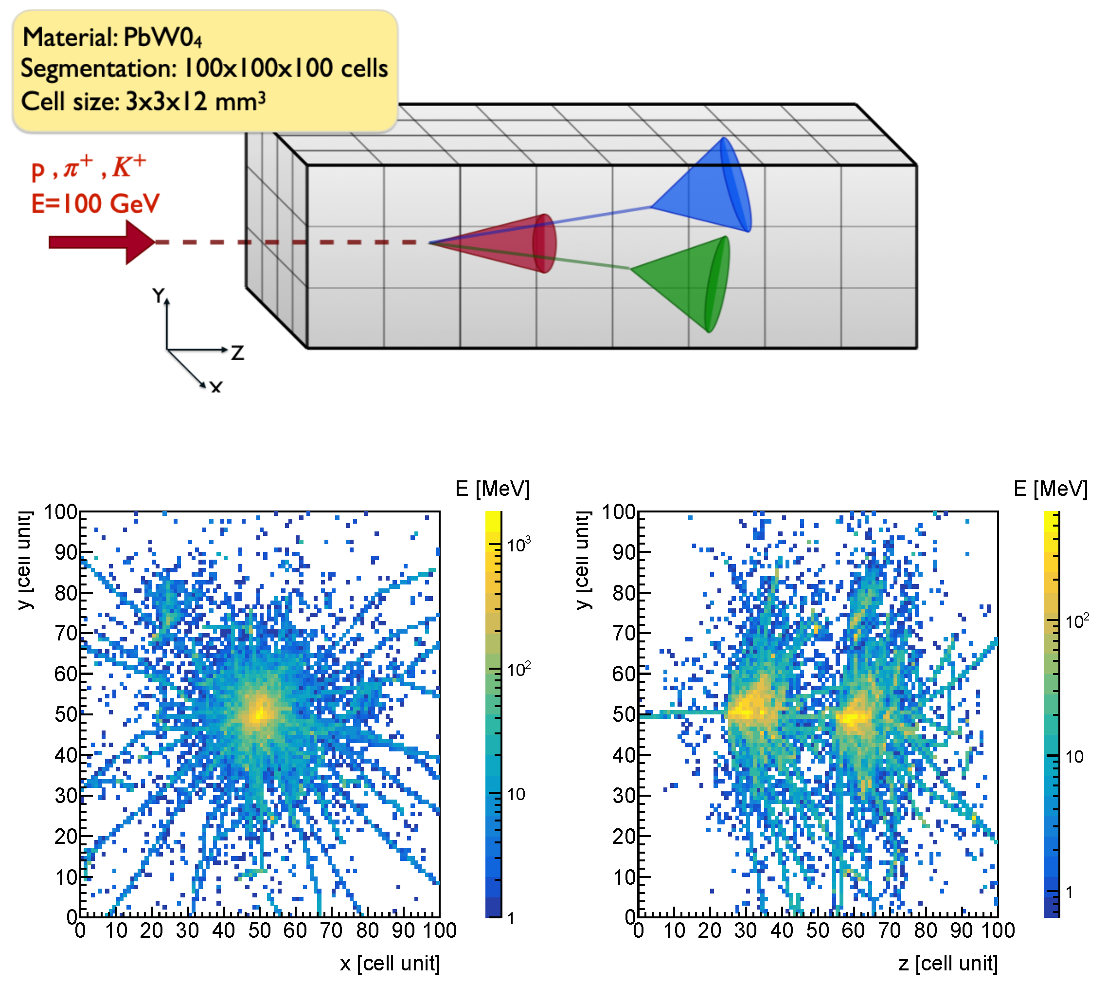
2. Simulation and Data Generation

In order to study the physical processes occurring inside the calorimeter, GEANT4 is used, specifically employing FTFP_BERT as the Reference Physics List [10,11,12]. The simulated primary particles are p, K + , and π + , each with energy equal to 100 GeV, and are generated at 3 m from the calorimeter surface. The particles enter the calorimeter perpendicularly, with the impinging position at the center of the calorimeter’s XY plane.
The experimental simulated setup consists of a homogeneous calorimeter made up of 100 × 100 × 100 cells constructed from Lead Tungstate ( PbWO 4 ) with dimensions of 3 × 3 × 12 mm 3 . Therefore, the total size of the calorimeter is 300 × 300 × 1200 mm 3 , which corresponds to a lateral width of 7.66 ρ M (Molière radii) and 5.92 λ I (interaction lengths), ensuring an average lateral containment of 100% and a longitudinal containment of approximately 87% (see Figure 1). In each simulated event, the following quantities are extracted through GEANT4’s SteppingAction:
  • PDG index: This refers to the identity of the particle that released the energy, and its value is encoded according to the Particle Data Group’s encoding;
  • PostStep TotalMomentum: This variable retrieves the total momentum of the particle after it has completed the current step in the simulation;
  • Delta Kinetic Energy: This variable is computed as the difference between the kinetic energy after and before the GEANT4 simulation step;
  • TotalEnergyDeposit: This variable retrieves the total energy deposited during the simulation step;
  • PostStep GlobalTime: This variable measures the GlobalTime (time since the beginning of the event) after the GEANT4 step.
  • Spatial coordinates of the cell that recorded the step: Each step is recorded by a cell, identified by a pair of indices: the cubelet index (representing a 10 × 10 × 10 region in the calorimeter) and the cell index (representing the cell within the cubelet). Both indices range from 0 to 99.
Some of the above listed quantities are inaccessible in a real experiment, whereas spatial coordinates, deposited energy, and global time can be considered as a high-accuracy version of the final variables observed in a real experiment.
To limit file size, only steps that satisfy the following conditions are saved:
TotalEnergyDeposit ≥ 1 keV OR Delta Kinetic Energy ≥ 1 keV. For each simulated particle ( p , π + , k + ), 50,000 events are generated, each with the same initial conditions. The produced event data are organized into 50 ROOT files, each containing 1000 events, where the information is stored as a ColumnWise Ntuple. This format ensures more efficient space management and speeds up read and write operations.

2.1. Time Smearing

To mimic a more realistic experimental setup, the recorded globalTime is preprocessed before using it to estimate the temporal variables describing the shower. To account for the finite time resolution of the detector, a smearing time of σ = 30 ps has been introduced, ensuring that the simulated detector is compatible with current technologies [13].

3. Definition of Sensitive Variables

To characterize energy showers within the calorimeter, it is essential to define a set of variables that encapsulate the key physical and geometric properties of the event. These variables are classified as global or local. Global variables represent the overall properties of the event, and serve as a baseline to describe the system in the absence of segmentation. In contrast, local variables are derived from the calorimeter’s segmentation, offering detailed spatial insights of the shower.
Before delving into the detailed description of the calculated variables, it is important to first define the properties extracted from each cell. These properties serve as the basis for the calculation of the descriptive variables.

3.1. Properties of Calorimeter Cells

Each calorimeter cell is characterized by three fundamental properties:
  • Position: The spatial coordinates of the cell within the calorimeter, which determine its location in the detector geometry.
  • Total absorbed energy: The total energy deposited in the cell during the event.
  • Cell Characteristic time: The timing information associated with a cell, defined as the weighted average of the times of all energy depositions within the cell, where the deposited energy serves as the weight:
    t cell = i E i c e l l t i c e l l i E i c e l l
    Here, E i c e l l represents the i-th energy deposition within the cell, and t i c e l l is the corresponding time. The sum is taken over all the energy depositions within the cell.

3.2. Global Variables

The three global variables considered are the following:
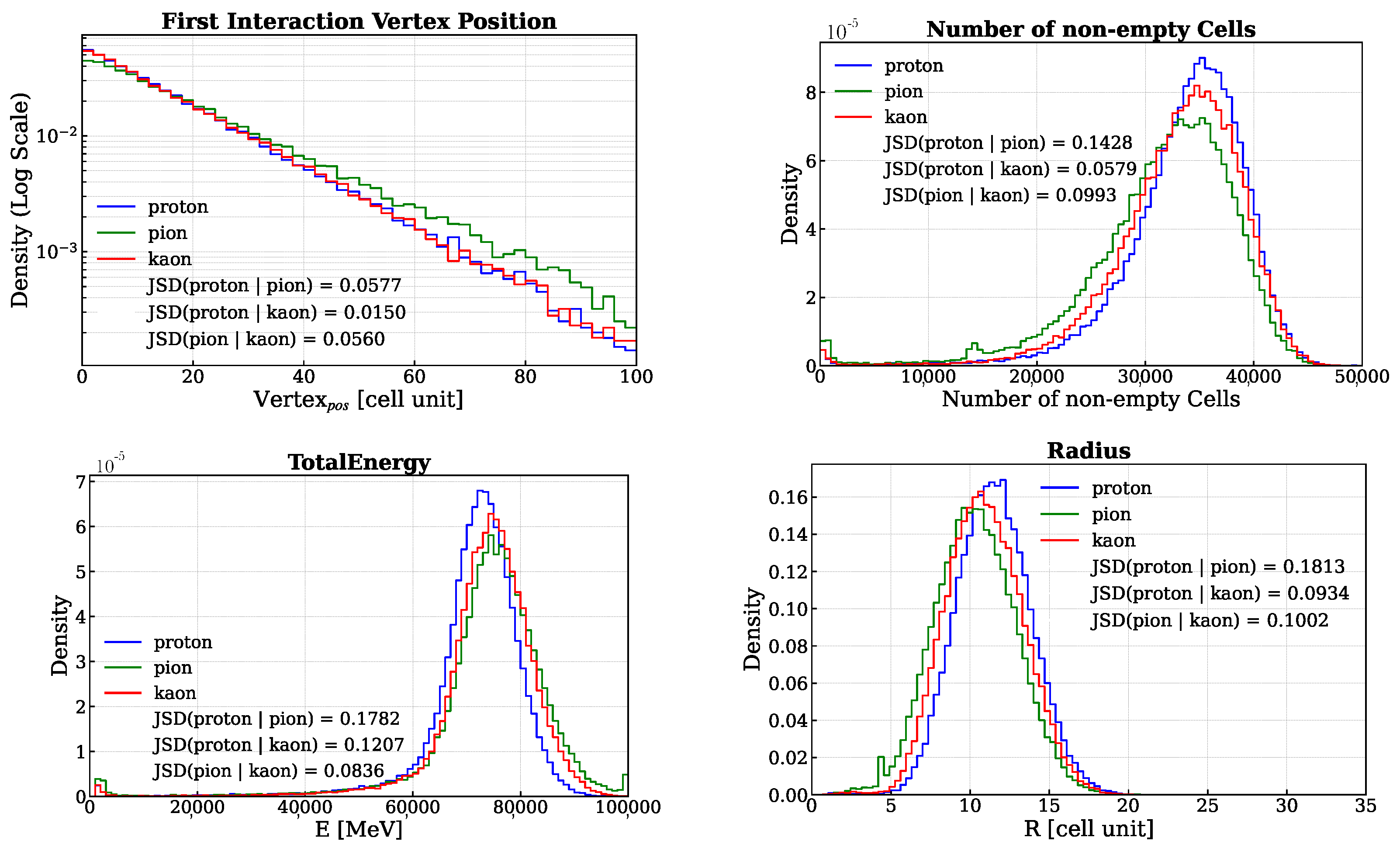
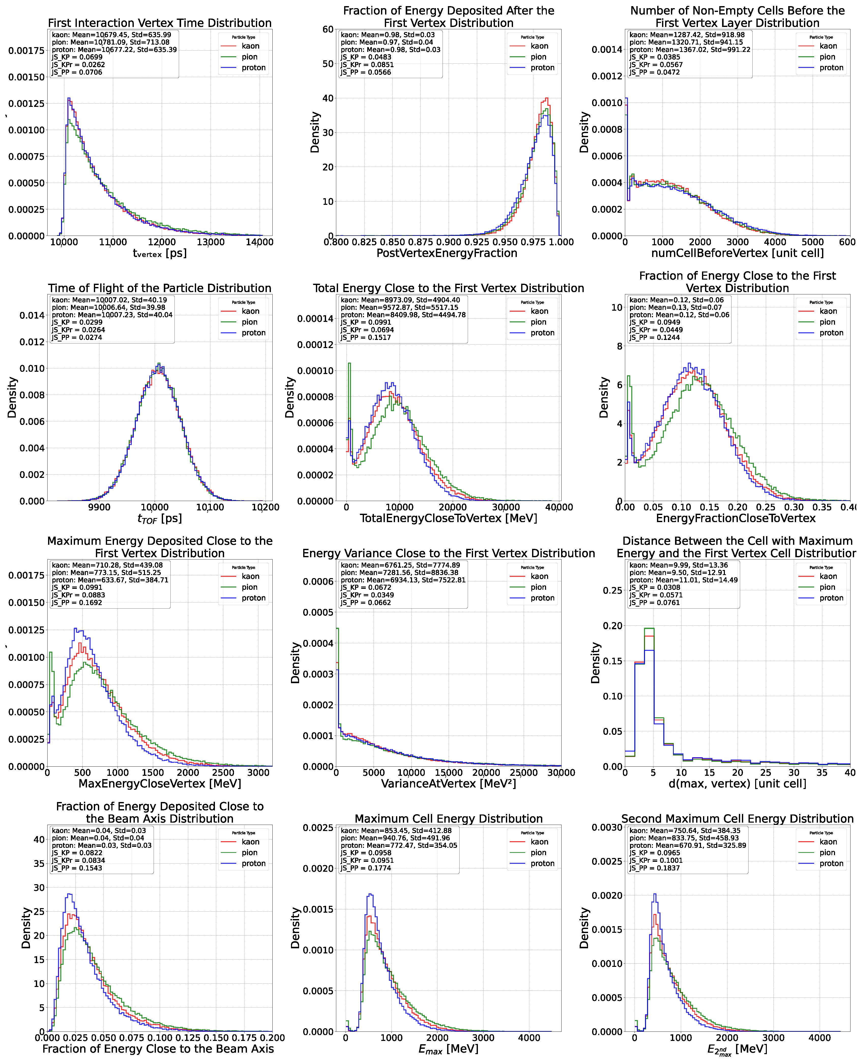
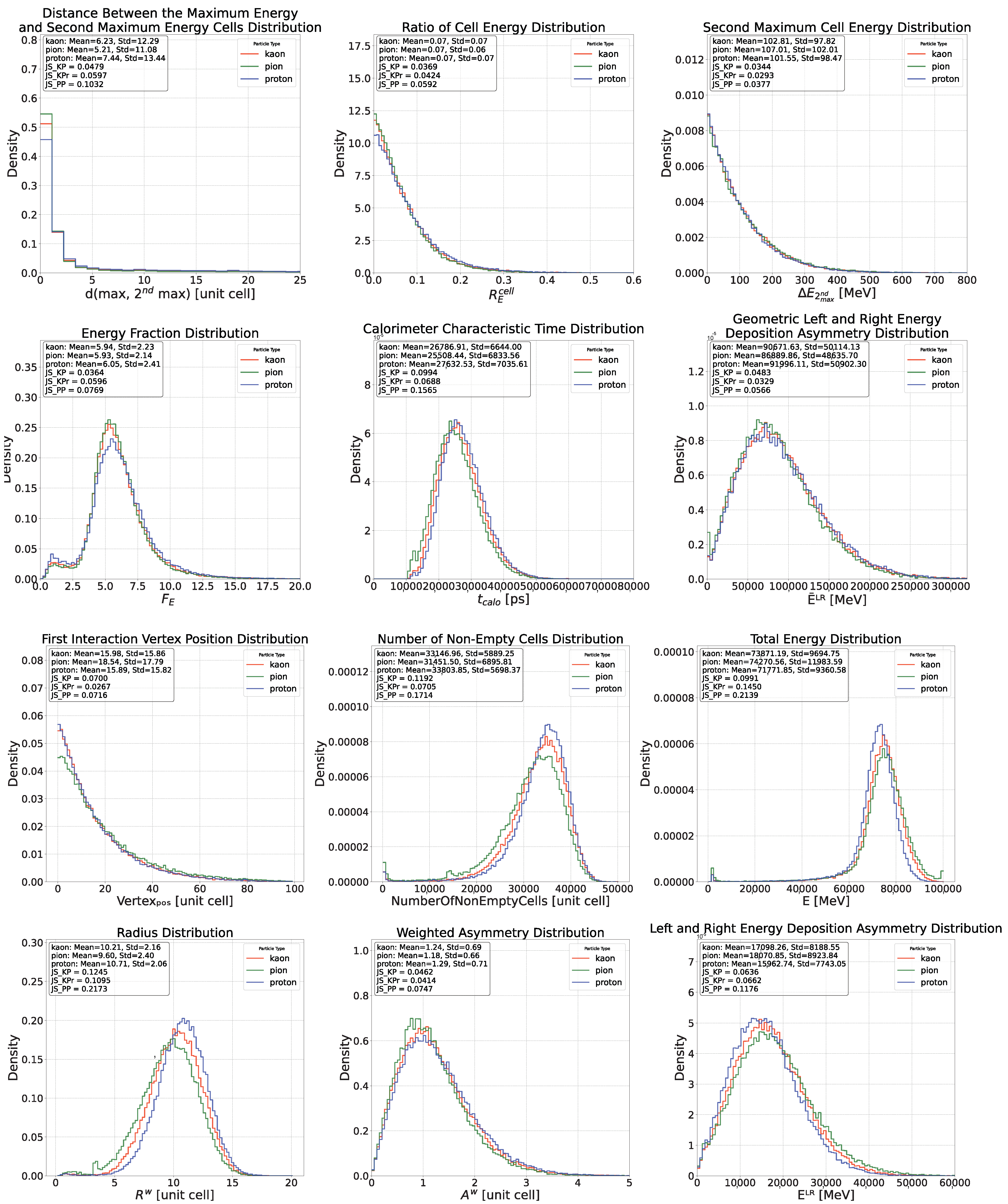
  • Total energy deposited in the calorimeter: In Figure 2, the corresponding distribution is displayed in the bottom-left corner.
  • Calorimeter characteristic time: The timing information associated with the calorimeter, defined as the weighted average of the characteristic times of all cells, where the energy deposited in each cell serves as the weight:
    t calo = cell E cell t cell cell E cell
    This property is computed using the cell properties, and for that reason, it could be considered a local variable. However, its meaning is global, as it corresponds to the mean signal time extracted from a homogeneous calorimeter.
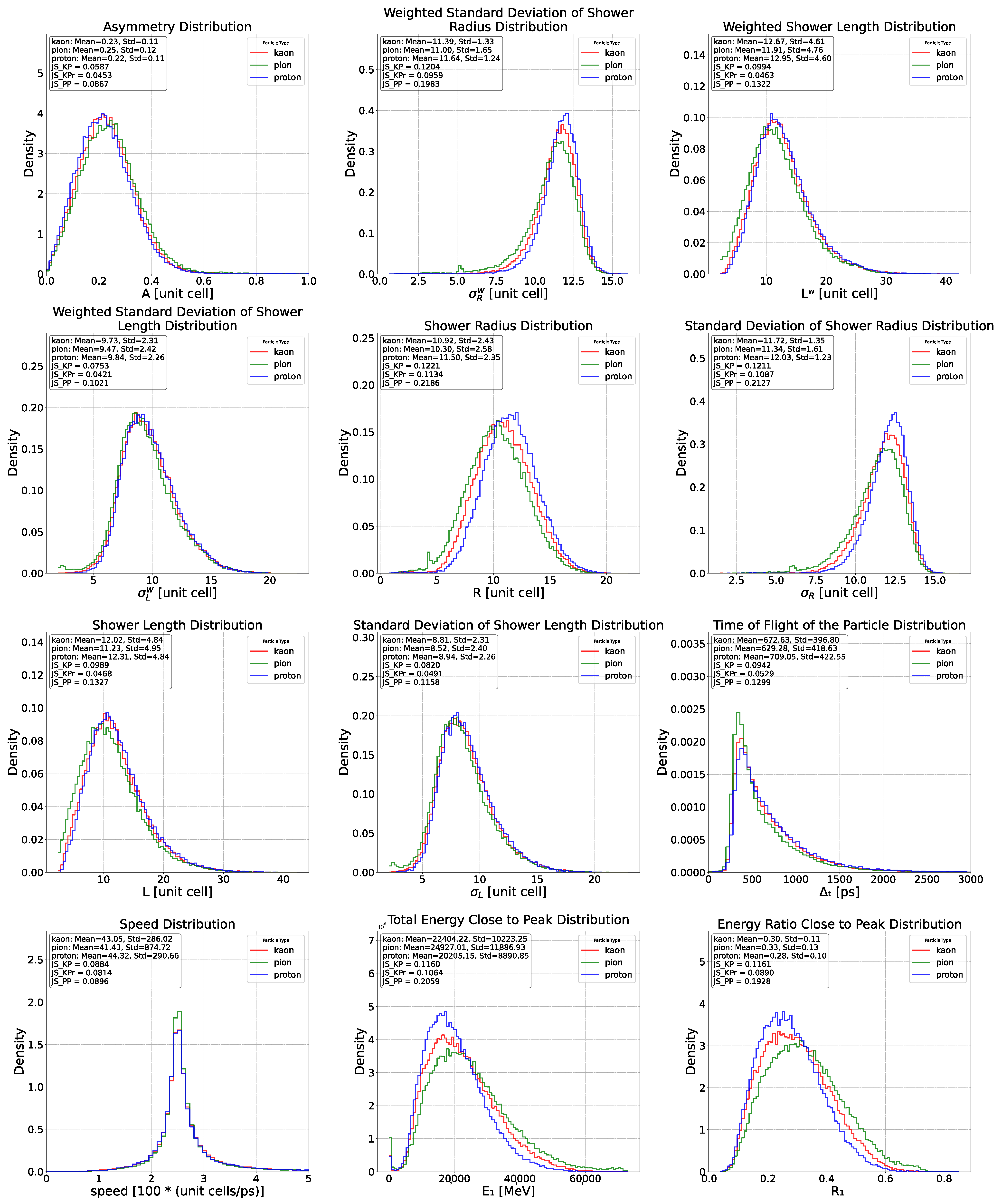
  • Time of flight of the particle: The time of flight (ToF) of the primary particle, hypothetically extracted from a tracker-like detector that is 3 m long and placed before the calorimeter. Assuming that it is possible to measure the creation time and the arrival time of the particle at the calorimeter interface with perfect resolution, this feature is extracted as follows:
    p = E 2 m 2 c 4 c
    v = ( p / E ) c 2
    t T O F = d / v
    where E and m are the total energy of the particle and its rest mass, respectively. Here d is the distance traveled by the particle and it is equal to 3 m; a 30 ps smearing is however added to time measurements later, see infra, Section 2.1.

3.3. Local Variables

The introduction of longitudinal and transverse segmentation in the calorimeter enables the study of the evolution of the energy shower as the particle interacts with the calorimeter. Based on this concept and considering the physical properties of the particles under examination, it is possible to define a set of local variables:
  • First nuclear interaction vertex position: The position of the first nuclear interaction vertex provides an indirect measure of the probability that a particle will interact with the medium through which it is passing. This probability, represented by the particle’s nuclear cross section, depends on the properties of the medium, the energy of the particle, and the particle’s identity. Therefore, when the first two factors are held constant, the position of the first interaction vertex becomes a variable sensitive to the particle’s identity. To determine this position, the First Nuclear Interaction Vertex Finder is used (see Appendix A). In Figure 2, the corresponding distribution is displayed in the top-left corner.
  • First interaction vertex time: The instant at which the first nuclear interaction vertex takes place can be defined as the characteristic time of the cell identified as containing that vertex.
  • Speed: Given the First Nuclear Interaction Vertex Position and the First Interaction Vertex Time, the particle speed is defined as the ratio between these two quantities.
  • Δ t : Given the First Interaction Vertex Time t V and the time when 50% of the total deposited energy is exceeded ( t 50 ), it is possible to define Δ t = t V t 50 .
  • Fraction of energy deposited after the first vertex: Referring only to longitudinal segmentation, the calorimeter can be described as a set of layers perpendicular to the direction of the primary particle. Based on this premise, the fraction of energy released after the primary interaction vertex is defined as the energy deposited in the cells located in the layers of the calorimeter that follow the layer containing the vertex.
  • Number of non-empty cells before the first vertex layer: Using the same logic applied to compute the Fraction of Energy Deposited after the First Vertex, it is also possible to count the number of non-empty cells in the layers preceding the one containing the vertex.
  • Number of non-empty cells: The total number of cells for which the deposited energy is greater than 0.1 MeV. In Figure 2, the corresponding distribution is displayed in the top-right corner.
  • Maximum cell energy: Maximum Cell Energy refers to the highest total energy deposited in the cells of the calorimeter.
  • Second maximum cell energy: This variable measures the total energy deposited in the calorimeter cells, representing the second highest value.
  • Total energy close to the first vertex and fraction of energy close to the first vertex: Once the cell of the primary vertex has been identified, it is possible to define a sphere with radius d, centered on the selected cell; for different studied segmentations d varies between 2 and 5 cell units. The total energy deposited in the cells within this sphere represents the Total Energy Close to the First Vertex. Thus it also represents a fraction of the total energy deposited in the calorimeter.
  • Maximum energy deposited close to the first vertex: Once the cell of the primary vertex has been identified, it is possible to define a sphere with radius d, centered on the selected cell; for different studied segmentations d varies between 2 and 5 cell units. The maximum energy near the primary vertex corresponds to the highest total energy deposited in one of the cells of the sphere.
  • Energy variance close to the first vertex: Once the cell containing the primary vertex has been identified, a transverse section cross-section of the calorimeter can be examined, encompassing all the cells within it. The individual energy values of these cells can then be used to calculate the variance of the energy deposited within the calorimeter slice centered on the cell containing the primary vertex.
  • Distance between the cell with maximum energy and the first vertex cell: By considering all the cells of the calorimeter, it is possible to define the distance between the cell containing the primary interaction vertex and the cell with the maximum energy deposition.
  • Distance between the maximum energy and second maximum energy cells: By considering all the cells of the calorimeter, it is possible to define the distance between the cells with the first and second maximum energy depositions.
  • Energy close to energy peak and fraction of energy close to energy peak: After the primary vertex, a peak of deposited energy is generated. The position of this peak can be determined using the energy peak finder (see Appendix B). Similar to the cell containing the primary vertex, a sphere with radius d (cell unit), centered on the cell containing the energy peak, can be defined. This sphere allows for the assessment of the total energy deposited around the peak, as well as the fraction of the total energy deposited within it.
  • Left and right energy deposition asymmetry: The impinging position of the primary particle can be considered the center of the reference system, so it is necessary to change the reference system from that of the simulation to the one just described.
    x * = x x c
    y * = y y c
    Once the new reference system has been adopted, it is possible to compare the left and right energy deposition. There are two methods: the standard definition ( E L R ) and the geometrical definition ( E ¯ L R ). The former is defined as follows
    E x L R = i = 1 N sgn ( x i * ) · E i where sgn ( x i * ) = 1 if x i * > 0 1 if x i * < 0 0 if x i * = 0
    E y L R = i = 1 N sgn ( y i * ) · E i where sgn ( y i * ) = 1 if y i * > 0 1 if y i * < 0 0 if y i * = 0
    E L R = ( E x L R ) 2 + ( E y L R ) 2
    The geometrical definition, on the other hand, is defined as the following:
    E ¯ x L R = i = 1 N x i * · E i
    E ¯ y L R = i = 1 N y i * · E i
    E ¯ L R = ( E ¯ x L R ) 2 + ( E ¯ y L R ) 2
    This definition involves the product of the position of the energy depositions and the energy deposits. The former is expressed in cell units, making it dimensionless. Consequently, the geometric definition yields pure energy values, expressed in MeV.
  • R E cell : The energy ratio R E c e l l is defined as the following
    R E c e l l = E m a x E 2 n d m a x E m a x + E 2 n d m a x
    Here, E m a x represents the maximum total energy deposited in one cell and E 2 n d m a x is the second maximum total energy.
  • Δ E cell : The energy Delta Δ E c e l l is the numerator of R E c e l l .
  • F E : The energy fraction is defined as the following
    F E = E   ( within up to ± N cells around E m a x ) E   ( within up to 1 cell around E m a x ) 1
    Here, N can be tuned and it defines a cube around the cell with the maximum total energy.

3.3.1. Physics-Based Observables

The slightly lower response of the calorimeter to protons compared to pions of the same energy can be attributed to the fact that, on average, a smaller fraction of the shower energy in proton-induced showers is carried by π 0 -mesons than in pion-induced ones. This difference arises because of the requirement of baryon-number conservation in nuclear interactions. When a proton undergoes its first nuclear interaction in the absorber material, the leading (most energetic) particle produced is typically a baryon. As this leading particle undergoes subsequent interactions, the most energetic produced particle remains likely to be a baryon. This conservation of baryon number limits the energy available for the production of π 0 , which generates the calorimeter signal. In contrast, pion-induced showers are not subject to this restriction, which allows more energy to be channeled into π 0 production [14].
The origin of these observed differences between proton and pion showers strongly suggests that the measurable effects are not limited to these particles. In particular, significant differences are also expected between kaon and pion showers. Similarly to baryon number conservation in proton showers, the strangeness quantum number is conserved by strong interactions that occur during kaon-induced showers. The strange (anti-)quark contained in the incident kaon is likely to be transferred to a highly energetic particle during each stage of the shower development [14].
The expected outcome is a broader lateral shower profile and a more symmetric signal distribution for protons and kaons compared to pion-induced showers. Furthermore, the electromagnetic fraction is higher for pions than for protons and kaons [14].
  • Fraction of energy deposited close to the beam axis: The differences in the fraction of calorimetric signal in the central tower can also be explained by this leading particle effect [14]. The leading particle carries a large fraction of the momentum of the incident particle. Therefore, it may be expected to travel almost in the same direction as the incident particle [14]. If this particle is a π 0 , it will thus generate a large signal in the central calorimeter tower. The soft π 0 ’s that constitute the signal from proton-induced showers are produced, on average, at larger angles than the leading particles [14]. As a result, the lateral profile of the energy deposition by the π 0 is wider for proton-induced showers than for pion-induced ones. Thus, the fraction of the total signal recorded in the central tower is, on average, smaller for protons and kaons than for pions [14].
  • Standard spatial observables: Each energy deposit position can be described by the position of the cell in which it occurred. Thus, it is possible to define the average position along the x, y and z axes of the laboratory reference system ( x ¯ , y ¯ , z ¯ ). With these quantities, the average radius of the energy shower (R) and the σ R are the following
    R = i = 1 N r i N with r i = ( x i x ¯ ) 2 + ( y i y ¯ ) 2
    σ R = i = 1 N r i 2 N R 2 with r i = ( x i x ¯ ) 2 + ( y i y ¯ ) 2
    In Figure 2, the R distribution is displayed in the bottom-right corner.
    Similarly, the average length of the energy shower (L) and its standard deviation are following
    L = i = 1 N l i N with l i = z i z ¯
    σ L = i = 1 N l i 2 N L 2 with l i = z i z ¯ .
  • Weighted spatial observables: Alternatively, the spatial observables can be calculated using the deposited energy as weight. This is how the standard spatial observables are modified once the deposited energy is also taken into account:
    R w = i = 1 N E i · r i i = 1 N E i with r i = ( x i x ¯ ) 2 + ( y i y ¯ ) 2
    σ R w = i = 1 N E i · r i 2 i = 1 N E i R w 2 with r i = ( x i x ¯ ) 2 + ( y i y ¯ ) 2
    L w = i = 1 N E i · l i i = 1 N E i with l i = z i z ¯
    σ L w = i = 1 N E i · l i 2 i = 1 N E i L w 2 with l i = z i z ¯ .
  • A and A w : The presence of asymmetries in the transverse profile of the shower can be estimated with the parameters A and A w . Similarly to the left-right energy asymmetry, the impinging position of the primary particle can be considered the center of the reference system. Once the new reference system has been adopted, the parameters A and A w can be calculated as follows:
    A = A x 2 + A y 2 with A x = i = 1 N x i * and A y = i = 1 N y i *
    A w = ( A x w ) 2 + ( A y w ) 2 with A x w = i = 1 N ( x i * · E i ) i = 1 N E i and A y w = i = 1 N ( y i * · E i ) i = 1 N E i
Figure 2. Selected feature distributions for proton, pion and kaons (cell size of 3 × 3 × 12 mm 3 ). For each particle, the corresponding Jensen-Shannon divergence is also reported to quantify the similarity between their respective distributions [15]. (Top-Left) First Nuclear Interaction Vertex Position. (Top-Right) Number of non-empty Cells. (Bottom-Left) Total energy deposited in the calorimeter. (Bottom-Right) Radius of the shower.
Particles 08 00058 g002

4. Study Setup and Methodology

To evaluate the performance of different classifiers, it is crucial to define a set of metrics that emphasize the discrimination power achieved by extracting descriptive features from the showers within the calorimeter. These performance metrics serve as quantitative tools to assess the model’s ability to generalize and make accurate predictions. They are indispensable for comparing different models and identifying areas for potential improvement. This section introduces the key metrics used in the study, along with a brief description of each. In addition, the various models tested in this work are presented.

4.1. Metrics

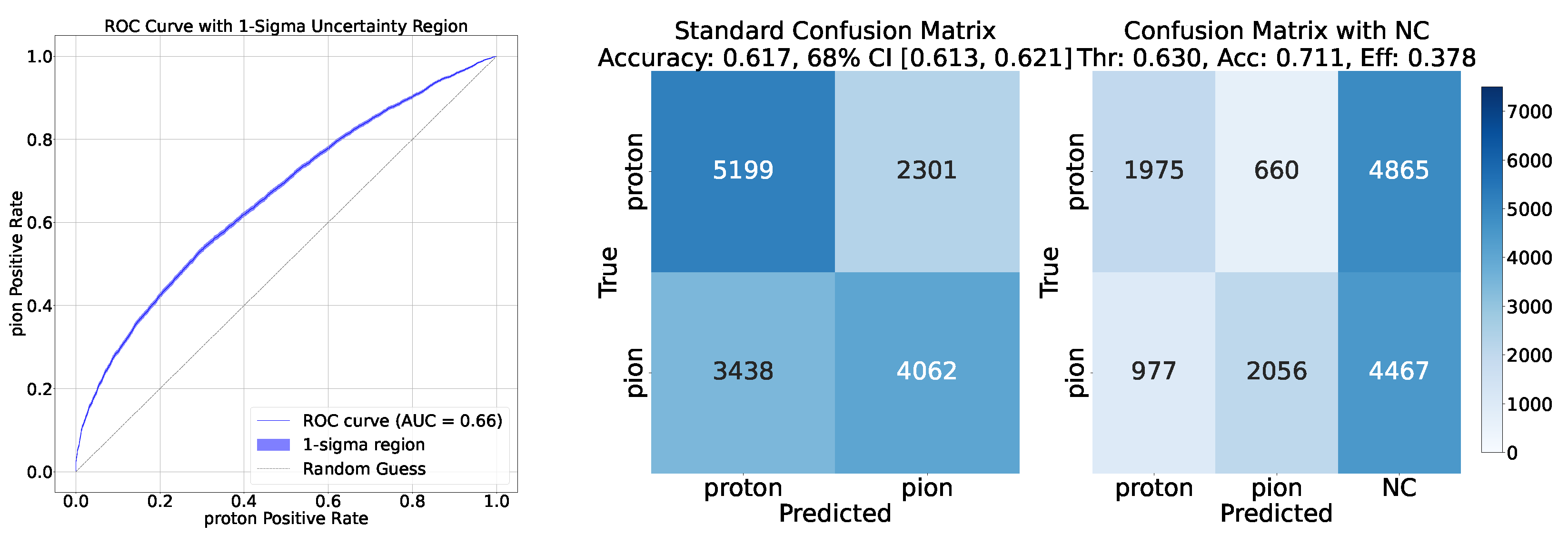
  • Confusion Matrix: The confusion matrix is a fundamental tool for evaluating classification models. The confusion matrix provides a foundation for deriving other metrics such as accuracy, precision, recall, and F1-score.
  • ROC Curve: The Receiver Operating Characteristic (ROC) curve is a graphical representation of a classification model’s performance across different threshold values. For example, when considering the p / π classification, it plots the Proton Positive Rate ( P R p ) against the Pion Positive Rate ( P R π ), defined as:
    P R p = number of protons classified as protons number of particles classified as protons , P R π = number of pions classified as pions number of particles classified as pions .
    The uncertainty associated with the ROC curve is calculated with Wald intervals for the binomial ratio, which is sufficient as the numbers at numerator and denominator are large and the ratio is not close to 0 or 1.
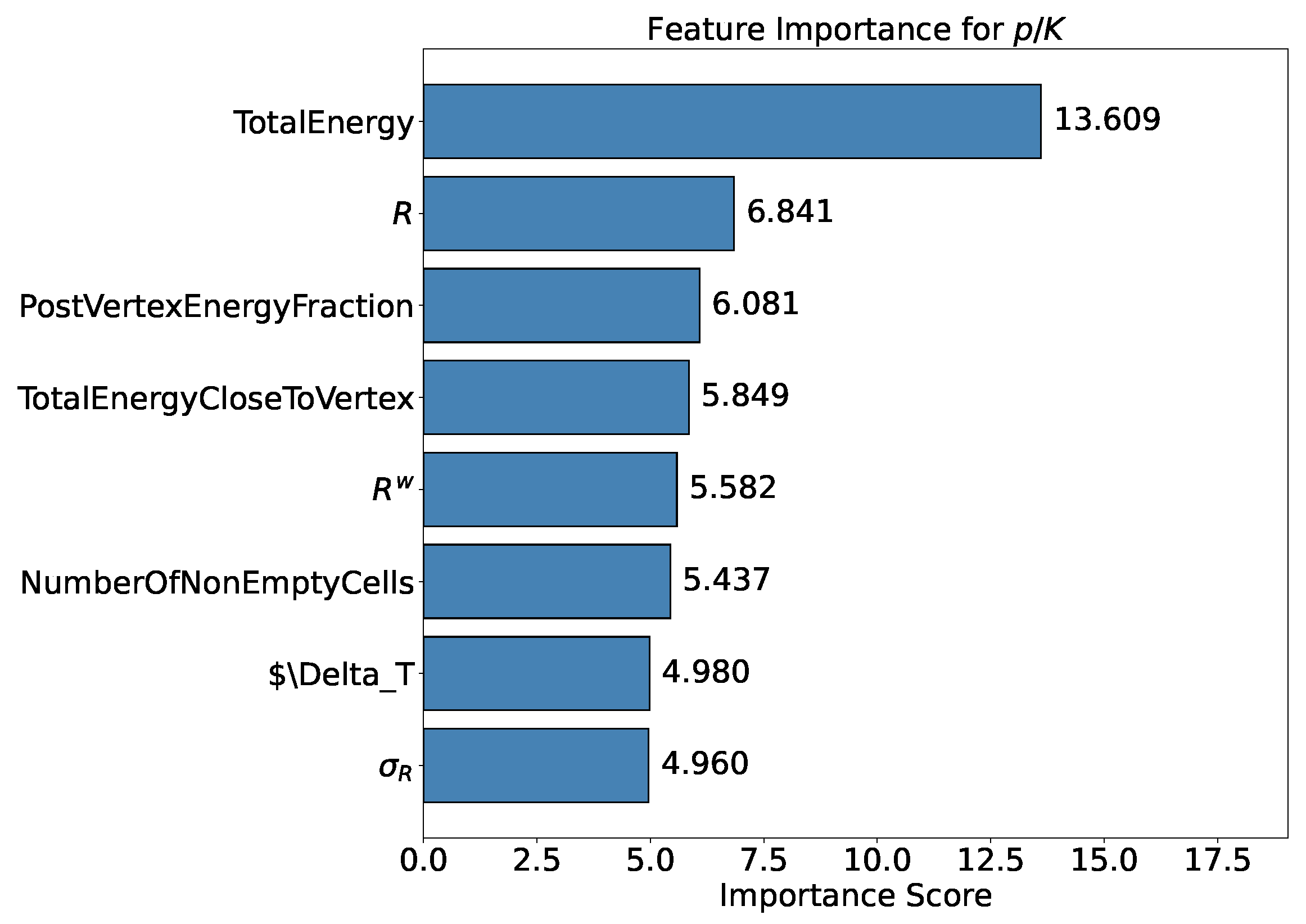
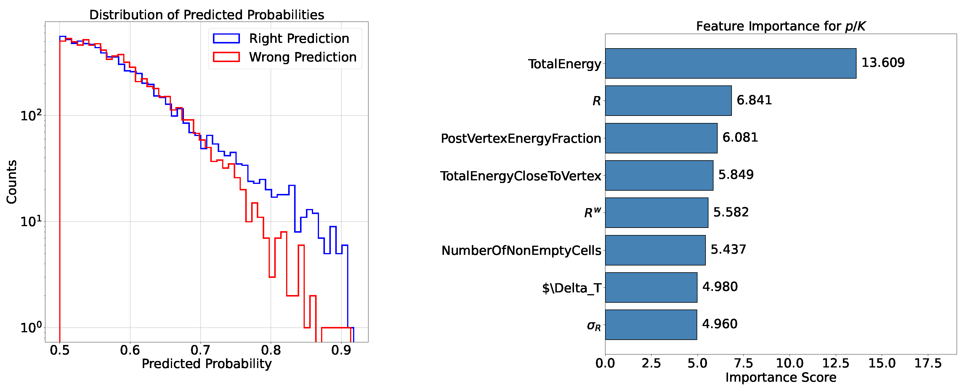
  • Feature Importance: Feature importance quantifies the contribution of each input variable to the model’s predictions. It helps identify the most relevant features for the task and provides insights into the underlying data. In the following analysis this metric is available when testing the XGBoost model. The chosen importance metric is “gain”, which represents the relative contribution of a feature to the model, calculated based on its impact across each tree. A higher gain compared to another feature signifies greater importance in the prediction. It measures the improvement in accuracy brought by a feature to the branches it influences: by adding a split on feature X, two new branches are created, each exhibiting higher accuracy than before, thereby reducing misclassifications.
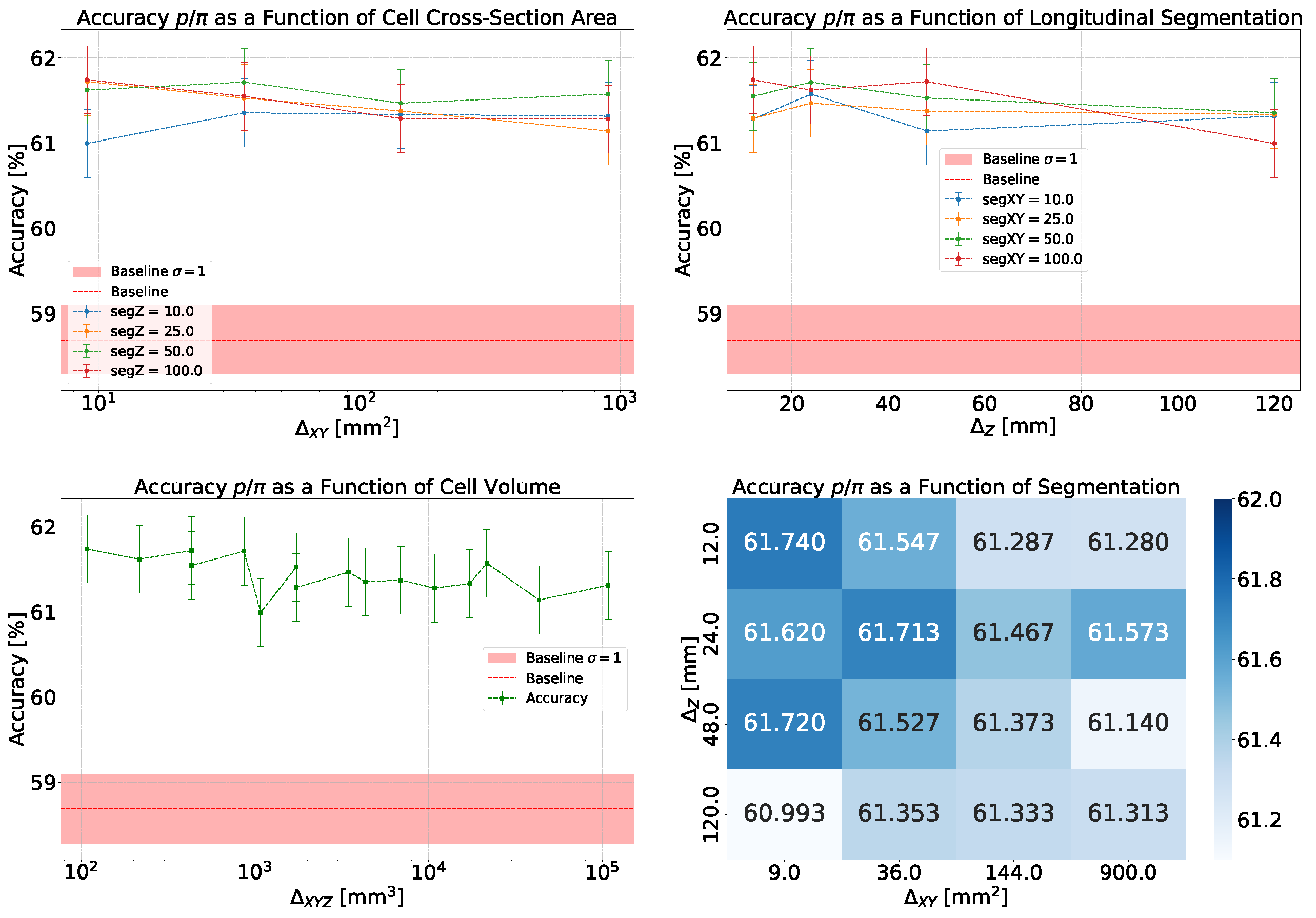
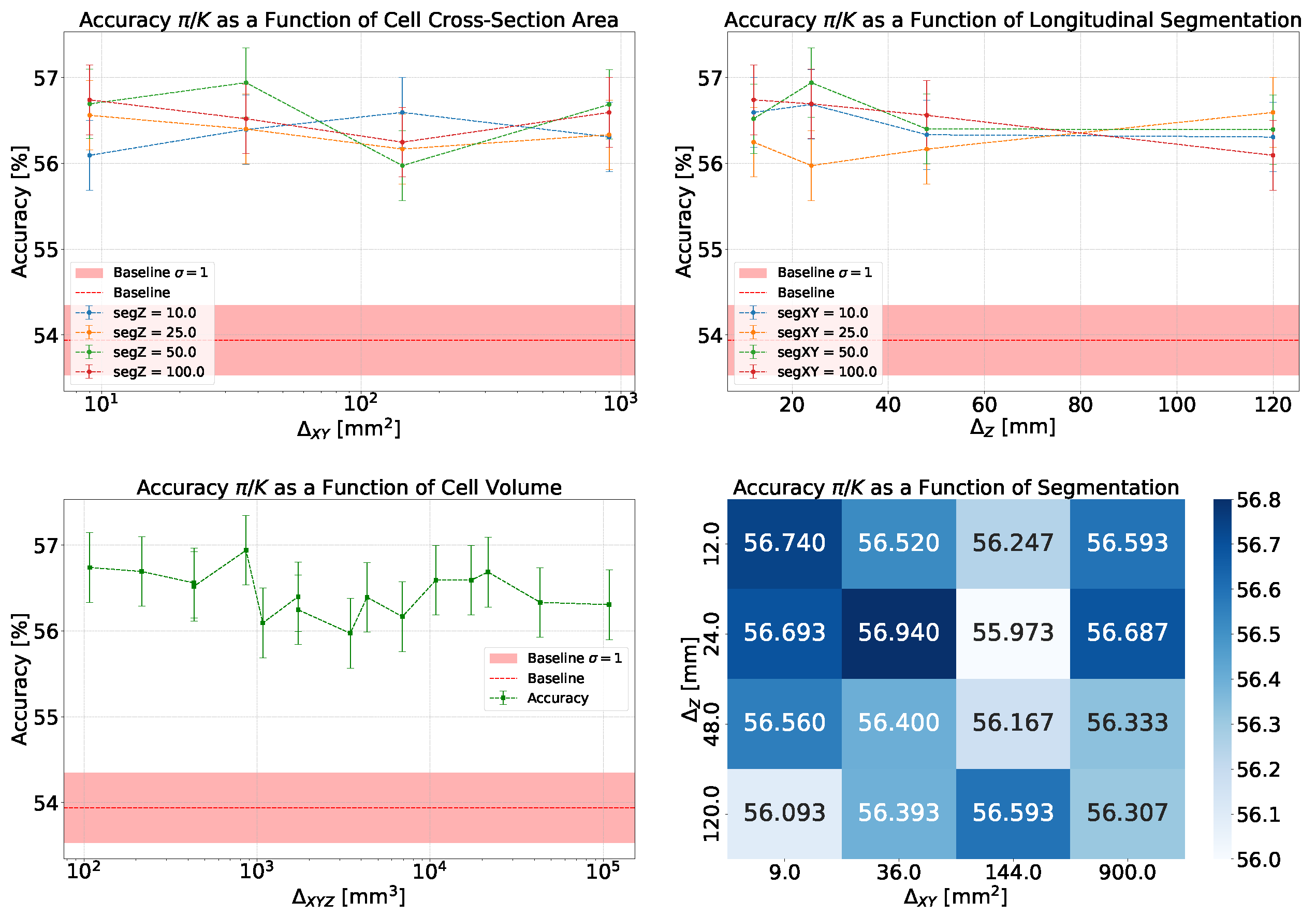
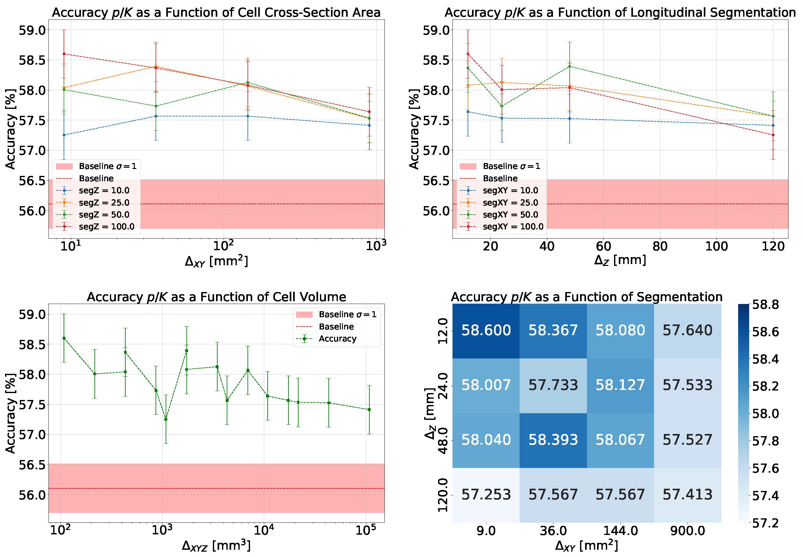
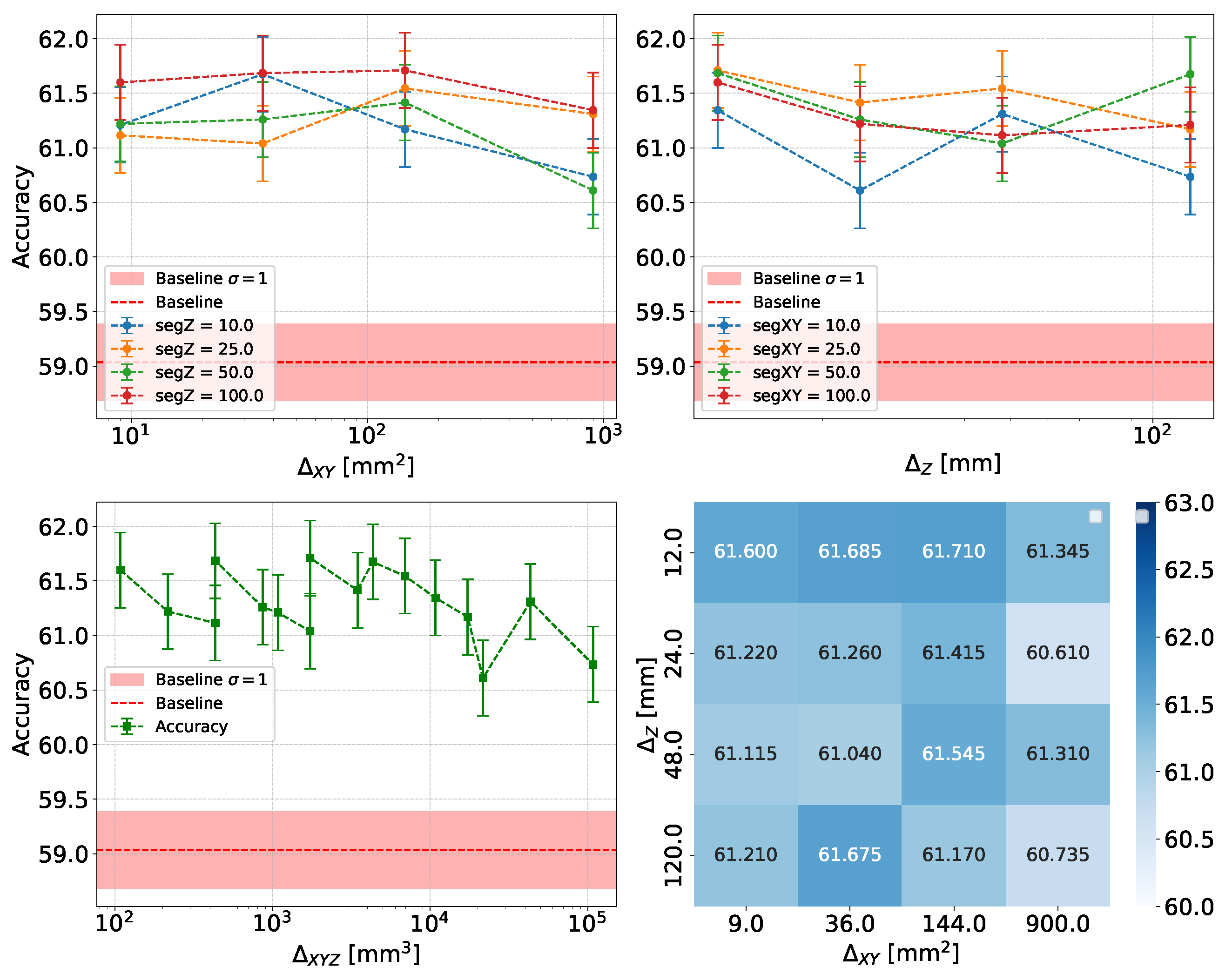
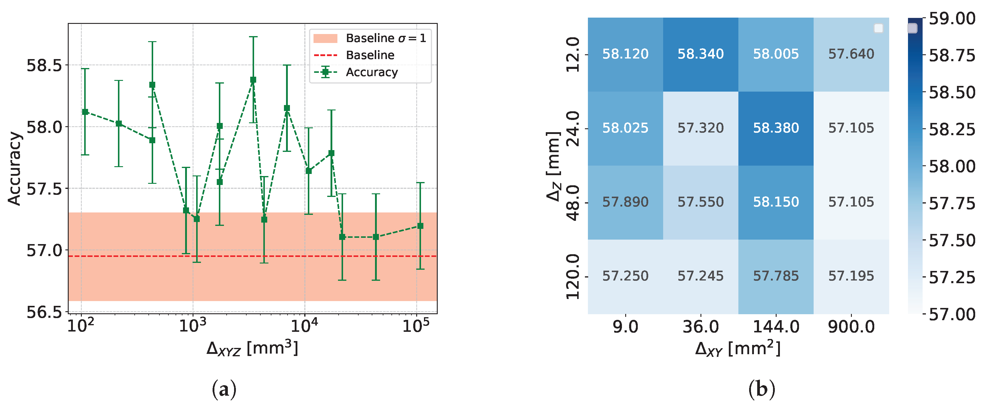
  • Accuracy and Efficiency: The models used for classifying showers into particle classes ( p / π , p / K , or π / K ) output pairs of values summing to 1, representing the probability that an event belongs to either the first or second class. For example, in the classification of protons and pions, the model might output a probability of 0.7 for a proton, meaning the probability for a pion would be 0.3.
    A threshold can be defined based on these probabilities to determine the reliability of the model’s output. By setting such a threshold, fewer outputs are considered reliable, reducing the algorithm’s efficiency, which refers to number of output that are reliable over the total number of inputs. However, this trade-off leads to improved accuracy, a measure of how well the model’s predictions match the true class labels, calculated as the proportion of correct predictions out of all predictions made. The accuracy and efficiency curves show how these metrics change with varying threshold values.
    Moreover, the accuracy values as a function of the calorimeter cell size are presented. This analysis is carried out for various configurations, with comparisons made by incorporating the uncertainty in the accuracy values. The uncertainty is estimated using the Clopper-Pearson interval, which provides a confidence interval for a binomial proportion. For an accuracy a, estimated over a sample of n observations with k successes, the confidence interval [ a low , a high ] at a confidence level of 1 α is defined as:
    a low = BetaInv α 2 , k , n k + 1 ,
    a high = BetaInv 1 α 2 , k + 1 , n k ,
    where BetaInv ( ) represents the inverse cumulative distribution function of the Beta distribution.

4.2. Machine Learning Strategy

Two different models were studied to conduct the following study. The first model was built using the XGBoost gradient boosting algorithm, while the second consists of a Fully Connected Deep Neural Network (DNN). Specifically, for each model, a hyperparameter tuning study was conducted using Grid Search.
For each classification task ( p / π , p / K , π / K ) the dataset consists of 100k events evenly split between the two particles under examination. It includes the features described in Section 3 and it is partitioned into 60% for training, 20% for validation, and 20% for evaluating the model’s accuracy.

4.2.1. XGBoost

XGBoost, or eXtreme Gradient Boosting, is a powerful machine learning algorithm under the ensemble learning category, specifically within the gradient boosting framework. It combines predictions from multiple decision trees to build a strong predictive model, using gradient descent optimization to minimize errors. Key features include its computational efficiency, ability to handle complex relationships, and regularization techniques to prevent overfitting.
Boosting is a technique where trees are built sequentially, with each tree correcting the errors of the previous one by learning from updated residuals. The base learners in boosting are weak learners with high bias and low predictive power, but their combination produces a strong learner that reduces both bias and variance. Unlike bagging methods like Random Forest, boosting uses smaller, shallow trees that are more interpretable. In order to find optimized parameters such as number of trees, learning rate, and tree depth a 3-fold cross-validation has been performed.
In order to obtain the output described in Section 4.1, the objective function should be set to binary:logistic.

4.2.2. Deep Neural Network

In addition to utilizing XGBoost, a fully connected Deep Neural Network (DNN) is used for classifying protons and pions. However, DNNs often struggle with highly imbalanced datasets and tabular data structures, as highlighted in Grinsztajn et al.’s findings [16]. This limitation arises because DNNs are generally less effective at capturing relationships in tabular data compared to tree-based models.
One effective way to mitigate these issues is through proper data preprocessing, such as standardizing the features. By using Scikit-learn’s StandardScaler, one can normalize the dataset to have a mean ( μ ) of zero and a standard deviation ( σ ) of one, ensuring that all features are on a similar scale. This helps DNNs converge more efficiently during training and can significantly improve performance, especially when the dataset is skewed.
Figure 3 illustrates the architecture utilized for implementing the Neural Network. The network consists of four hidden layers with [96, 32, 16, 4] neurons in each respective layer. Each hidden layer employs a LeakyRelu activation function along with Batch Normalization. Additionally, 15% random dropout is applied to prevent overfitting. The final layer output is passed through Softmax activation function to transform the raw scores into probability scores. (Note: The Softmax function is not used explicitly here, but is implicitly included in PyTorch’s CrossEntropyLoss loss function.)
Table 1 presents the optimal hyperparameters identified through Grid Search. During training, a dynamic learning rate is adopted, which makes learning more stable [17].

5. Results

This section presents the results achieved by the considered models. Using the metrics detailed in Section 4.1, the performance was evaluated for three distinct classification tasks. Specifically, for each simulated particle pair ( p / π , p / K , and π / K ), the study examines the impact of segmentation in a calorimeter compared to a homogeneous calorimeter which serves as baseline. Additionally, the analysis explores how this contribution evolves with changes in cell size.

5.1. XGBoost

Using the setup described in Section 4.2, the results of the study conducted for the three different classification tasks are reported below.

5.1.1. p / π Classification

As explained in Section 3.3.1, the conservation of baryon number for protons and the dominant branching ratio of neutral pions for charged pions are the key factors used to investigate the differences between showers produced by protons and pions. The consequences of these differences are manifested in some of the features, particularly the transverse size of the showers, represented by the radius and the fraction of energy released along the direction of the interacting particle, i.e., the shower core. In addition, the higher radius of protons induces a higher probability of nuclear interaction with the calorimeter material than for pions. From this it follows that on average a smaller fraction of the pion energy will be deposited in the calorimeter because 100% containment of charged pions would require a larger longitudinal dimension of the calorimeter.
These assumptions are confirmed by the ranking of the features that contribute the most to identifying the primary particle (see Section 4.1). Figure 4 shows that the features related to the transverse development of the shower are the highest, along with the total deposited energy. However, the position of the primary interaction vertex does not play a dominant role in distinguishing between the two particle species. This result may be due to the fact that, in order to be sensitive to this quantity in a PbWO 4 calorimeter, it is necessary to use cells with a longitudinal size smaller than 12 mm. Additionally, it is important to note that the exact position of the interaction vertex is not directly accessible in a real experiment and it is identified using an algorithm with an accuracy of less than 100% (see Appendix A for details on the algorithm’s definition and performance analysis). The physical insights offered by the XGBoost model represent a key advantage of its application. Interpreting the results within a physical context not only enhances the understanding of the underlying processes but also, as in this case, provides valuable guidance for defining the practical requirements to be applied in the design of future detectors.
Another significant result concerns the study of the model’s output. As described in Section 4.1, the output can be interpreted as a pair of probabilities indicating the likelihood that the sample is a proton or a pion. By taking the higher of the two probabilities and defining this value as the winning probability, two distributions can be constructed. One distribution corresponds to the winning probability when the classification is correct, while the other represents the winning probability when the sample is misclassified.
In Figure 5, it can be seen that these values are, by definition, greater than 0.5. Moreover, above a certain winning probability threshold, the model consistently returns the correct class. This finding is noteworthy because it suggests the possibility of defining a confidence level that the model must meet to produce reliable output.
This observation can also be related to Figure 5, where the accuracy and efficiency curves described in Section 4.1 are shown. Increasing the confidence level reduces the model’s efficiency but simultaneously improves its accuracy. Additionally, the impact of this choice on individual particles can be observed: raising the threshold shows that pions are more easily discriminated.
The analysis proceeds by evaluating the accuracy achieved in distinguishing protons from pions. The right plot of Figure 6 presents two confusion matrices. The first matrix illustrates the maximum accuracy achieved at full efficiency, with the corresponding ROC curve shown on the left side of the same figure. The second matrix represents the accuracy obtained when the threshold on the model’s output is set to the value that yields the highest achievable accuracy for protons.
The analysis concludes with a study on the impact of segmentation compared to the use of a homogeneous, non-segmented calorimeter and the effect of cell size on the model’s performance. In the top-left panel of Figure 7, the accuracy is shown as a function of the cell cross-section for various longitudinal segmentations, while in the top-right panel, the accuracy is plotted against the longitudinal segmentation size for different transverse segmentations. Both plots highlight an improvement in performance with the introduction of segmentation, increasing the baseline accuracy from 58.7% to an average value of 61.4%.
In the bottom-left panel of Figure 7, the dependence of accuracy on the cell volume is shown, revealing a decreasing trend as the cell volume increases. This result confirms that introducing smaller-volume cells can provide a better description of showers within the calorimeter.
In all the graphs of accuracy versus cell dimensions, the quoted accuracy values are strongly correlated because of the use of the same input data for training, validation, and testing. Therefore the variability shown by the accuracy results over cell dimensions is more significant than what the uncertainty bars seem to imply. Finally, the bottom-right panel of Figure 7 shows the accuracy achieved for various configurations of longitudinal and transverse segmentations.

5.1.2. π / K Classification

Similarly to the p / π classification case discussed above, there are physical reasons that could potentially create a difference between a shower produced by a charged pion and one produced by a charged kaon. Just as the baryon number is conserved in proton showers, the strangeness quantum number is conserved in the strong interactions occurring in kaon-induced showers. The strange (anti-)quark contained in the incident particle is likely to be transferred to a highly energetic particle in each generation of the shower development. The production of π 0 ’s in kaon showers is therefore limited by a mechanism very similar to that in proton showers. This can lead to showers that are wider and more symmetric compared to those produced by pions.
As highlighted in Figure 8 on the left, this is confirmed by the presence of variables describing the transverse development of the shower, such as the radius, among the top-ranking features. It is worth noting the presence of the number of non-empty cells, which indicates a difference between the two types of showers. In particular, looking at Figure 2 it can be seen that the number of non-empty cells for pions is, on average, smaller than that for kaons.
In the analysis of the winning probability distributions, it becomes clear that the principle outlined in Section 5.1.1 does not apply here, as no threshold exists where correct predictions consistently outnumber incorrect ones (see Figure 8 on the right).
Finally, observing the contribution of segmentation to the particle identification power π / K , an improvement is noted in this case as well (see Figure 9, top). On the other hand, the trend with respect to cell volume does not seem to follow a defined pattern, suggesting that exploring smaller cell sizes might be necessary to fully resolve the showers induced by pions and kaons (see Figure 9, bottom left).

5.1.3. p / K Classification

This third analysis yields results that can be considered intermediate compared to the two previous analyses. By examining the distribution of winning probabilities (see Figure 10, left), an inflection point can be observed where the distribution of correct predictions surpasses that of incorrect ones. However, this outcome is not as beneficial as the one described in Section 5.1.1, as it would result in a considerable loss of efficiency in exchange for only a slight improvement in accuracy.
In Figure 10 on the right, it can be noted that the total energy released dominates among the input features, suggesting that the impact of segmentation in this case is less significant. Finally, the trend of accuracy relative to the baseline and its dependence on cell size are observed. In the bottom left of Figure 11, a decreasing trend is visible as the cell volume increases, and the same trend can be observed for both transverse and longitudinal segmentation (see Figure 11, top).

5.2. Deep Neural Network

This section discuss the results obtained using Deep Neural Network (DNN). The DNN model is trained on the NVIDIA GeForce RTX 4090 GPU, completing 180 epochs in approximately 25 min.
Figure 12 shows the training and validation loss, as well as the training and validation accuracy. It is evident that both the loss and accuracy saturate within the range of epochs studied.
Figure 13 show the results obtained using a Deep Neural Network (DNN) for the classification of p / π . The plots illustrate how accuracy varies with changes in the granularity of the calorimeter. Uncertainty bars in the DNN graphs of accuracy are computed using Clopper-Pearson interval with α = 0.32 using Equation (27) (see Section 4.1 for more details). Along with p / π classification, DNN model for the classification between π / K and p / K has been tested.
Figure 14 and Figure 15 illustrate the relationship between granularity and accuracy for p / K and π / K classifications, respectively. A slight decrease in accuracy is observed as the cell volume increases. However, this decline is not monotonic, and considering the error bars, the variation appears minimal. The specific reasons for this behavior are discussed in Section 5.1.1, Section 5.1.2 and Section 5.1.3.
When comparing the performance of the XGBoost model and Deep Neural Networks (DNN), it is observed that both models yield similar results, effectively eliminating the possibility of selection bias. However, XGBoost stands out as a more feasible and cost-effective option in terms of computational efficiency. While DNNs are highly effective for tensor-based data, the tabular data structure used in this context aligns better with the strengths of XGBoost. Additionally, XGBoost offers a simpler implementation and has the advantage of being an interpretable model, as it provides explicit feature importance. In contrast, DNNs determine feature importance implicitly, making their interpretability more challenging. This makes XGBoost not only a computationally efficient choice but also a model that offers greater insights into the data.

6. Related Work

High-Granularity Calorimeters will be the natural choice in future particle physics experiments at high-luminosity colliders, where the number of produced particles in each interaction may further increase from the already large value they have in today’s LHC collisions. This will generate a large amount of data, which is difficult to process using traditional methods due to the high computational demands. Recently, machine learning algorithms have become useful tools for handling this data, especially for tasks like particle classification and regression. For example, as shown in [18], neural networks have demonstrated significant progress in energy regression and particle classification for HGCAL. They simulated CMS and ATLAS calorimeter geometry and used both electromagnetic and hadron calorimeter to seperate γ / π 0 and e / π ± . The GlueX experiment at Jefferson Lab used neural networks to separate background photons from hadron interactions and signal photons from ω -meson decays. This highlights the power of neural networks in rejecting background noise, especially for neutral particles [19]. Many existing methods employ Convolutional Neural Networks (CNNs), which are well-suited for image-based data, including visualizations of calorimetric showers. However, calorimetric showers inherently lack a natural ordering, unlike images which are structured grids. This unordered nature of calorimetric data makes point cloud representations a more suitable and intuitive choice.
As demonstrated in Ref. [20], point cloud representations effectively capture the spatial and energy distribution of calorimetric showers. These representations enable the use of permutation-invariant architectures like DeepSets [21], which are specifically designed to handle unordered data. This approach allows for a more natural modeling of calorimetric showers and has been successfully applied to accelerate their simulation, offering both computational efficiency and accuracy compared to traditional methods.

7. Conclusions

High granularity is today an important requirement for calorimeters in high-energy physics applications, due to the possibility to identify sub-jets from the decay of hadronically decaying, boosted heavy particles within wide jets, as well as to due to the benefits of the use of particle-flow techniques in event reconstruction. In this work we have set out to study the possibility of distinguishing charged hadrons by the topological and time structure of their energy deposition in a homogeneous calorimeter of extremely high granularity, as a complementary piece of information that together with the requirements of boosted-jet tagging and particle-flow reconstruction may better inform the optimal design of future instruments. By studying a lead tungstate calorimeter block impinged by protons, pions, and kaons of positive charge and of 100 GeV of energy, we studied the distinguishability of these three classes through high-level features constructed with the information available from a hypothetical readout of energy and time of energy deposition in individual cells of very small size. By progressively merging cells into larger units we tried to ascertain how the harvested information would degrade in a less granular calorimeter.
Our findings indicate that increased granularity enhances the accuracy of particle identification, marking a promising starting point for further investigations. Although the simulation takes into account only particles at 100 GeV, and therefore the possibility of identifying different charged hadrons is reduced, the results show the presence of a small discrimination power offered by granularity. The trends presented in Section 5 demonstrate that an accuracy of approximately 62% can be achieved for p / π classification, while the performance is worse for the other classification tasks. Despite the significant uncertainties in the data, an overall decreasing trend in accuracy is observed as the cell volumes increase. Therefore, this provides a first indication of the potential advantages that increased granularity could offer for future experiments and related analyses.
As reported in Section 5, features related to the transverse development of the shower are important, while the primary interaction vertex does not play a dominant role. In principle, this result might not be expected, as the primary vertex is closely related to the interaction cross section between the primary particle and the material. We believe this outcome can be explained by the energy of the particles as, at high energies, the cross sections are similar. This suggests that the discrimination power could be more pronounced at lower energies.
Our results reflect the current status of our investigations; they are still preliminary, as they do not conclusively ascertain yet what is the attainable, ultimate state-of-the-art level of discrimination of the different particle species, nor the scale of cell volume below which the required information is preserved. To achieve those goals it will be necessary to couple the high-level feature approach with a convolutional neural network or graph-based network, which can extract the hierarchical structure of shower evolution because representing cell relationships through graphs would allow for a comprehensive description of the shower, capturing both its global structure and local properties; the combined information of low-level and high-level information is guaranteed to offer results of closer to ultimate power. In addition, a study of a full spectrum of different particle energies in the range typical of collider physics applications [1 GeV–1 TeV], and consideration of negatively-charged particles (antiprotons, negative pions and kaons), neutral ones (neutrons, K L 0 ) as well as deuterons and anti-deuterons will provide a better overall picture of the use of granular calorimeters for event reconstruction and particle identification.
Regarding the choice of a lead tungstate calorimeter with 3 × 3 × 12 mm 3 sized cells, we believe that, although this configuration may not be realizable in a physical system it can serve as useful test point for investigation of information extraction in high granular calorimeters. State-of-the-art calorimeters indicate that the community is moving towards granular designs incorporating both crystal and fiber scintillators. Several R&D studies highlight the feasibility of small calorimeter units, as demonstrated by the SPACAL prototype [22].
We intend to pursue the above studies in future work; regardless of the interim nature of presented results, we believe they already show how useful particle identity information is extractable from the construction of informative high-level features that summarize the properties of the patterns of deposited energy and their time structure. For this reason we propose this methodology as possible application of granularity in future granular calorimeters.

Author Contributions

Conceptualization, A.D.V. and T.D.; Methodology, A.D.V. and T.D.; Software, A.D.V., A., J.W., E.L., F.N. and X.T.N.; Validation, A.D.V., A. and J.W.; Formal analysis, A.D.V., A., E.L. and X.T.N.; Data curation, A.D.V., A. and E.L.; Writing—original draft, A.D.V., A. and T.D.; Writing—review & editing, A.D.V., A., M.A. (Max Aehle), M.A. (Muhammad Awais), A.B., R.C., L.C., T.D., N.R.G., R.K., J.K., E.L., F.N., X.T.N., F.S., K.S., P.V. and J.W.; Visualization, A., M.A. (Max Aehle), M.A. (Muhammad Awais), A.B., R.C., L.C., T.D., N.R.G., R.K., J.K., E.L., F.N., X.T.N., F.S., K.S., P.V. and J.W.; Supervision, L.C., T.D., N.R.G., R.K., J.K., F.N., F.S. and P.V.; Funding acquisition, T.D. and P.V. All authors have read and agreed to the published version of the manuscript.

Funding

The work by TD and FS was partially supported by the Wallenberg AI, Autonomous Systems and Software Program (WASP) funded by the Knut and Alice Wallenberg Foundation. The work by MA and FS was partially supported by the Jubilee Fund at the Luleå a University of Technology. The work by PV was supported by the “Ramón y Cajal” program under Project No. RYC2021-033305-I funded by the MCIN MCIN/AEI/10.13039/501100011033 and by the European Union NextGenerationEU/PRTR. JK is supported by the Alexander-von-Humboldt foundation.

Data Availability Statement

The resources used for the analysis can be found on the following GitHub page (accessed on 19 April 2025): https://github.com/andread3vita/TowardPIDwithGranularCalorimeters.

Conflicts of Interest

The authors declare no conflict of interest.

Appendix A. First Nuclear Interaction Vertex Finder

The First Nuclear Interaction Vertex Finder algorithm is designed to identify the index of the first “peak” in a vector of values, based on a specified threshold criterion. Below is a detailed breakdown of its components and functionality.

Appendix A.1. Inputs and Parameters

The function takes the following inputs:
  • energyCoordinates: A vector representing the spatial energy coordinates.
  • energyDeposition: A vector representing the energy deposited at each coordinate.
  • threshold: The initial threshold used to detect the peak in the energy profile.

Appendix A.2. Step-by-Step Algorithm Overview

  • Energy Profile Calculation The algorithm processes the interactions to construct an energy profile along the z-dimension:
    • Spatial coordinates and energy deposition (E) are retrieved for each interaction.
    • Energy contributions are accumulated into z-slices within the XY window range.
    • To improve peak detection, the energy profile is smoothed using a moving average filter.
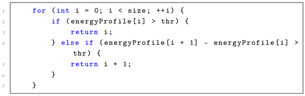
  • First Pass: Initial Peak Detection In the first pass, the algorithm scans the energyProfile to locate the first peak using the original threshold:
    • Iterate through the elements of the energy profile:
      Particles 08 00058 i001
    • The algorithm identifies significant peaks in a sequence by comparing the values of consecutive elements. If an element surpasses a predefined threshold, its index is immediately returned as a peak. Alternatively, if the difference between two consecutive elements exceeds the threshold, the index of the second element is returned, marking it as the peak.
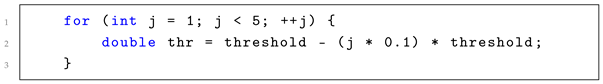
  • Second Pass: Threshold Reduction If no peak is found in the first pass, the threshold is gradually reduced, and the search is repeated:
    • Decrease the threshold by 10% in each iteration:
      Particles 08 00058 i002
    • Perform the peak detection search with the new threshold:
      Particles 08 00058 i003
  • Handling Cases with No Peak If no peak is detected after both passes, the function returns −1, indicating that no significant peaks were found in the vector.

Appendix A.3. Summary of Behavior

  • The function employs a greedy approach, returning the index of the first detected peak in the energy profile.
  • By gradually reducing the threshold, the function becomes more sensitive to smaller variations in the data, improving peak detection in cases of low-energy deposition.
  • If no peak is identified after both search passes, the function returns −1, indicating that no peak meets the specified criteria.

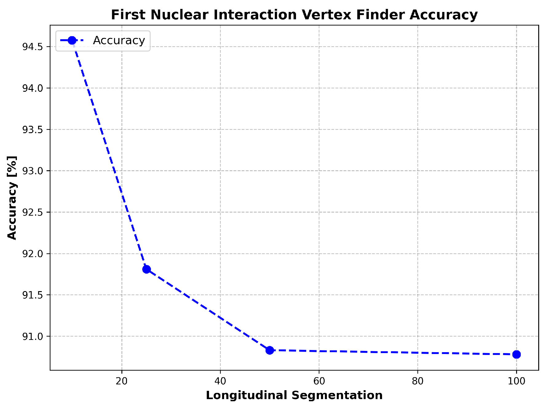
Appendix A.4. Performance Evaluation

To evaluate the algorithm’s performance, an accuracy metric is defined. This metric corresponds to the ratio between the number of events where the absolute difference between the trueZvertex and the recoZvertex is less than 2 cell units, and the total number of events. Based on this definition, the algorithm’s performance was analyzed for various longitudinal segmentations.
As shown in Figure A1, the accuracy is always above 90%, with a minimum value of 90.78% when the segmentation is set to 100 cells along the z axis.
Figure A1. Accuracy of First Nuclear Interaction Vertex Finder as a function of the longitudinal segmentation.
Particles 08 00058 g0a1

Appendix B. Energy Peak Finder

The Energy Peak Finder function is designed to analyze events, identifying the most significant peak in the energy deposition profiles along the X, Y, and Z axes. Below is a step-by-step explanation of the function and its operations.

Appendix B.1. Inputs and Parameters

The function accepts the sphere_radius as parameter. It defines the radius of the sphere centered on the cell containing the energy peak.

Appendix B.2. Step-by-Step Algorithm Overview

  • Histograms Creation: Two 2D histograms (hist_cell_zy and hist_cell_zx) are created to represent energy deposits in the Z-Y and Z-X planes, respectively. These histograms are filled on the basis of the event data.
  • Energy Profile Along Z-Axis and Peak Detection: The energy deposition data are projected along the Z-axis:
    • A projection of the hist_cell_zy histogram onto the Z axis is stored in projZ.
    • TSpectrum::Search is used to find peaks in projZ with a threshold of 0.1 [23].
    • The positions of the detected peaks along the Z-axis are stored in peaksZ.
    • The peaks are sorted in increasing order of associated energy, and the highest energy one is finally stored.
    In most analyzed events the algorithm finds a single peak; cases when multiple peaks compete for being classified as the first event vertex are very rare; the highest-energy one is anyway used.
  • Peak Filtering and Search in X and Y Projections: Given the Z peak position, the function performs the following steps:
    • Filters the hist_cell_zx and hist_cell_zy histograms based on the Z peak position.
    • Projects the filtered histograms onto the X and Y axes, respectively, creating projX and projY.
    • Searches for peaks in the X and Y projections using TSpectrum::Search [23].
    • If multiple peaks are found in X or Y, the algorithm selects the most prominent peak by comparing the peak intensities.
  • Energy Accumulation Around Peaks: The function accumulates the energy deposition values around the detected peak:
    • For each energy deposition in the event, the 3D position is converted to cell coordinates.
    • The proximity of the energy deposition to the detected peaks is evaluated, and the energy is added if the energy deposition is within the sphere defined by sphere_radius.

Appendix B.3. Results

Finally, the function returns a vector that contains the energy and the energy ratio of the most significant peak.

Appendix C. Feature Distributions for Proton, Pion and Kaons

Figure A2. These figures present the distributions of all features used in the analysis (cell size of 3 × 3 × 12 mm 3 ). The results are shown for each particle, and the Jensen-Shannon Divergence is reported for each particle pair to quantify the similarity between their respective distributions.
Particles 08 00058 g0a2
Figure A3. These figures present the distributions of all features used in the analysis (cell size of 3 × 3 × 12 mm 3 ). The results are shown for each particle, and the Jensen-Shannon Divergence is reported for each particle pair to quantify the similarity between their respective distributions.
Particles 08 00058 g0a3
Figure A4. These figures present the distributions of all features used in the analysis (cell size of 3 × 3 × 12 mm 3 ). The results are shown for each particle, and the Jensen-Shannon Divergence is reported for each particle pair to quantify the similarity between their respective distributions.
Particles 08 00058 g0a4

References

  1. Wing, M. Precise measurement of jet energies with the ZEUS detector. arXiv 2000, arXiv:hep-ex/0011046. [Google Scholar]
  2. Qu, H.; Gouskos, L. Jet tagging via particle clouds. Phys. Rev. D 2020, 101, 056019. [Google Scholar] [CrossRef]
  3. Dreyer, F.; Qu, H. Jet tagging in the Lund plane with graph networks. J. High Energy Phys. 2020, 2021, 52. [Google Scholar] [CrossRef]
  4. The ATLAS Collaboration. Transformer Neural Networks for Identifying Boosted Higgs Bosons Decaying into b b ¯ and c c ¯ in ATLAS. Technical Report; CERN: Geneva, Switzerland, 2023. [Google Scholar]
  5. Kasieczka, G. Boosted Top Tagging Method Overview. arXiv 2018, arXiv:1801.04180. [Google Scholar]
  6. The CMS Collaboration. Particle-flow reconstruction and global event description with the CMS detector. J. Instrum. 2017, 12, P10003. [Google Scholar] [CrossRef]
  7. Thomson, M. Particle flow calorimetry and the PandoraPFA Algorithm. Nucl. Instrum. Methods Phys. Res. Sect. A Accel. Spectrometers Detect. Assoc. Equip. 2009, 611, 25–40. [Google Scholar] [CrossRef]
  8. Bilki, B.; Repond, J.; Xia, L.; Eigen, G.; Thomson, M.A.; Ward, D.R.; Benchekroun, D.; Hoummada, A.; Khoulaki, Y.; Chang, S.; et al. Pion and proton showers in the CALICE scintillator-steel analogue hadron calorimeter. J. Instrum. 2015, 10, P04014. [Google Scholar] [CrossRef]
  9. Verhelst, M.; Bahai, A. Where Analog Meets Digital: Analog-to-Information Conversion and Beyond. IEEE Solid-State Circuits Mag. 2015, 7, 67. [Google Scholar] [CrossRef]
  10. Allison, J.; Amako, K.; Apostolakis, J.; Arce, P.; Asai, M.; Aso, T.; Bagli, E.; Bagulya, A.; Banerjee, S.; Barrand, G.; et al. Recent developments in Geant4. Nucl. Instrum. Methods Phys. Res. Sect. A Accel. Spectrometers Detect. Assoc. Equip. 2016, 835, 186–225. [Google Scholar] [CrossRef]
  11. Allison, J.; Amako, K.; Apostolakis, J.; Araujo, H.; Dubois, P.A.; Asai, M.; Barrand, G.; Capra, R.; Chauvie, S.; Chytracek, R.; et al. Geant4 developments and applications. IEEE Trans. Nucl. Sci. 2006, 53, 270. [Google Scholar] [CrossRef]
  12. Agostinelli, S.; Allison, J.; Amako, K.A.; Apostolakis, J.; Araujo, H.; Arce, P.; Asai, M.; Axen, D.; Banerjee, S.; Barrand, G.; et al. Geant4—A simulation toolkit. Nucl. Instrum. Methods Phys. Res. Sect. A Accel. Spectrometers Detect. Assoc. Equip. 2003, 506, 250–303. [Google Scholar] [CrossRef]
  13. Perez-Lara, C.; Wetzel, J.; Akgun, U.; Anderson, T.; Barbera, T.; Blend, D.; Cankocak, K.; Cerci, S.; Chigurupati, N.; Cox, B.; et al. Study of time and energy resolution of an ultra-compact sampling calorimeter (RADiCAL) module at EM shower maximum over the energy range 25 GeV ≤ E ≤ 150 GeV. arXiv 2024, arXiv:2401.01747. [Google Scholar] [CrossRef]
  14. Akchurin, N.; Ayan, S.; Bencze, G.L.; Chikin, K.; Cohn, H.; Doulas, S.; Dumanoǧlu, I.; Eskut, E.; Fenyvesi, A.; Ferrando, A.; et al. On the differences between high-energy proton and pion showers and their signals in a non-compensating calorimeter. Nucl. Instrum. Methods Phys. Res. Sect. A Accel. Spectrometers Detect. Assoc. Equip. 1998, 408, 380–396. [Google Scholar] [CrossRef]
  15. Lin, J. Divergence measures based on the Shannon entropy. IEEE Trans. Inf. Theory 1991, 37, 145–151. [Google Scholar] [CrossRef]
  16. Grinsztajn, L.; Oyallon, E.; Varoquaux, G. Why do tree-based models still outperform deep learning on tabular data? arXiv 2022, arXiv:2207.08815. [Google Scholar]
  17. Li, X.; Orabona, F. On the Convergence of Stochastic Gradient Descent with Adaptive Stepsizes. arXiv 2019, arXiv:1805.08114. [Google Scholar]
  18. Belayneh, D.; Carminati, F.; Farbin, A.; Hooberman, B.; Khattak, G.; Liu, M.; Liu, J.; Olivito, D.; Pacela, V.B.; Pierini, M.; et al. Calorimetry with deep learning: Particle simulation and reconstruction for collider physics. Eur. Phys. J. C 2020, 80, 688. [Google Scholar] [CrossRef]
  19. Barsotti, R.; Shepherd, M. Using machine learning to separate hadronic and electromagnetic interactions in the GlueX forward calorimeter. J. Instrum. 2020, 15, P05021. [Google Scholar] [CrossRef]
  20. Acosta, F.T.; Mikuni, V.; Nachman, B.; Arratia, M.; Karki, B.; Milton, R.; Karande, P.; Angerami, A. Comparison of point cloud and image-based models for calorimeter fast simulation. J. Instrum. 2024, 19, P05003. [Google Scholar] [CrossRef]
  21. Zaheer, M.; Kottur, S.; Ravanbakhsh, S.; Poczos, B. Deep Sets. In Advances in Neural Information Processing Systems; Curran Associates, Inc.: Red Hook, NY, USA, 2017; Volume 30. [Google Scholar]
  22. An, L.; Auffray, E.; Betti, F.; Dall’Omo, F.; Gascon, D.; Golutvin, A.; Guz, Y.; Kholodenko, S.; Martinazzoli, L.; De Cos, J.M.; et al. Performance of a spaghetti calorimeter prototype with tungsten absorber and garnet crystal fibres. Nucl. Instrum. Methods Phys. Res. Sect. A Accel. Spectrometers Detect. Assoc. Equip. 2023, 1045, 167629. [Google Scholar] [CrossRef]
  23. Silagadze, Z. A new algorithm for automatic photopeak searches. Nucl. Instrum. Methods Phys. Res. Sect. A Accel. Spectrometers Detect. Assoc. Equip. 1996, 376, 451–454. [Google Scholar] [CrossRef]
Figure 1. (Top) Illustration of the interaction of a simulated charged hadron with a PbWO 4 . (Bottom) the energy distribution of a proton shower projected in the XY and ZY planes.
Particles 08 00058 g001
Figure 3. Deep Neural Network architecture used for classification of hadrons.
Particles 08 00058 g003
Figure 4. Top 8 most important features used by the XGBoost model in the p / π classification (cell size of 3 × 3 × 12 , mm 3 ), ranked in descending order of significance. Each bar represents a feature, with its length proportional to its contribution, measured using the “gain” metric.
Particles 08 00058 g004
Figure 5. Analysis of the winning probability and its impact on accuracy and efficiency values (cell size of 3 × 3 × 12 , mm 3 with XGBoost). (Top-Left) Distribution of the winning probability, categorized into winning probabilities with correct classification (in blue) and winning probabilities with incorrect classification (in red). (Top-Right) Accuracy and efficiency curves considering both protons and pions. (Bottom-Left) Accuracy and efficiency curves for protons. (Bottom-Right) Accuracy and efficiency curves for pions.
Particles 08 00058 g005
Figure 6. (Left) p / K classification ROC curve. The uncertainty region is computed as described in Section 4.1. (Right) Confusion matrices illustrating XGBoost’s performance with a cell size of 3 × 3 × 12 , mm 3 : confusion matrix at full efficiency and when the threshold on the model’s output is set to the value corresponding to the highest achievable accuracy for protons. Particles whose classification confidence falls below the reliability threshold are labeled as ’Not Classified’ (NC).
Particles 08 00058 g006
Figure 7. Summary of results for p / π classification with XGBoost. (Top-Left) Dependence of accuracy on cell cross section for different longitudinal segmentations. (Top-Right) Dependence of accuracy on cell length section for different transverse segmentations. (Bottom-Left) Dependence of accuracy on cell volume. (Bottom-Right) Accuracy for different longitudinal and transverse segmentation configurations. Because of the use of the same input data, the reported accuracy values are correlated.
Particles 08 00058 g007
Figure 8. Analysis with the XGBoost model for the π / K classification (cell size of 3 × 3 × 12 mm 3 ). (Left) Top 8 most important features used by the XGBoost model in the π / K classification, ranked in descending order of feature importance. Each bar represents a feature, with its length proportional to its contribution, measured using the “gain” metric. (Right) Analysis of the winning probability and its impact on accuracy and efficiency values. Distribution of the winning probability, categorized into correct classification (blue) and incorrect classification (red).
Particles 08 00058 g008
Figure 9. Summary panels for π / K classification with XGBoost. (Top-Left) Dependence of accuracy on cell cross section for different longitudinal segmentations. (Top-Right) Dependence of accuracy on cell length section for different transverse segmentations. (Bottom-Left) Dependence of accuracy on cell volume. (Bottom-Right) Accuracy for different longitudinal and transverse segmentation configurations. Because of the use of the same input data, the reported accuracy values are correlated.
Particles 08 00058 g009
Figure 10. Analysis with the XGBoost model for the p / K classification (cell size of 3 × 3 × 12 mm 3 ). (Left) Distribution of the winning probability, categorized into correct classification (blue) and incorrect classification (red). (Right) Top 8 most important features used by the XGBoost model in the p / K classification, ranked in descending order of significance.
Particles 08 00058 g010
Figure 11. Summary results on p / K classification with XGBoost. Studies on the dependence of the accuracy on cell cross section, longitudinal segmentation and volume. Because of the use of the same input data, the reported accuracy values are correlated.
Particles 08 00058 g011
Figure 12. Training and validation accuracy, along with training and validation loss.
Particles 08 00058 g012
Figure 13. Summary of classification results for the p / π with DNN. The (top-left) panel shows the variation in accuracy with changes in transverse (XY) segmentation for a highly granular calorimeter while fixing longitudinal segmentation (Z). The (top-right) panel demonstrates how accuracy changes with variations in longitudinal (Z) segmentation while keeping the XY segmentation constant. The (bottom-left) panel illustrates accuracy variations with changes in the overall volume of calorimeter cells. Finally, the (bottom-right) panel displays an accuracy matrix, summarizing accuracy values for different datasets. Because of the use of the same input data, the reported accuracy values are correlated.
Particles 08 00058 g013
Figure 14. p / K classification results using DNN: (a) Accuracy variation with changes in cell volume (b) Accuracy matrix for different cell dimensions. Because of the use of the same input data, the reported accuracy values are correlated.
Particles 08 00058 g014
Figure 15. π / K classification results using DNN: (a) Accuracy variation with changes in cell volume (b) Accuracy matrix for different cell dimensions. Because of the use of the same input data, the reported accuracy values are correlated.
Particles 08 00058 g015
Table 1. Main parameters used in the neural network, sourced from PyTorch’s library.
ParameterSetting or Value
Batch size128
Type of loss functionCrossEntropyLoss
Weight decay0.001
Learning rate (initial)0.0009
Learning rate (schedule) lr = lr 1 + weight_decay · ( epoch ) 2.5
OptimizerAdamW
Disclaimer/Publisher’s Note: The statements, opinions and data contained in all publications are solely those of the individual author(s) and contributor(s) and not of MDPI and/or the editor(s). MDPI and/or the editor(s) disclaim responsibility for any injury to people or property resulting from any ideas, methods, instructions or products referred to in the content.

