All articles published by MDPI are made immediately available worldwide under an open access license. No special
permission is required to reuse all or part of the article published by MDPI, including figures and tables. For
articles published under an open access Creative Common CC BY license, any part of the article may be reused without
permission provided that the original article is clearly cited. For more information, please refer to
https://www.mdpi.com/openaccess.
Feature papers represent the most advanced research with significant potential for high impact in the field. A Feature
Paper should be a substantial original Article that involves several techniques or approaches, provides an outlook for
future research directions and describes possible research applications.
Feature papers are submitted upon individual invitation or recommendation by the scientific editors and must receive
positive feedback from the reviewers.
Editor’s Choice articles are based on recommendations by the scientific editors of MDPI journals from around the world.
Editors select a small number of articles recently published in the journal that they believe will be particularly
interesting to readers, or important in the respective research area. The aim is to provide a snapshot of some of the
most exciting work published in the various research areas of the journal.
The TomOpt software package is designed to optimise the geometric configuration and the specifications of detectors intended for muon scattering tomography, an imaging technique exploiting cosmic-ray muons. The software employs an end-to-end differentiable pipeline that models the interactions of muons with detectors and scanned volumes, infers properties of the scanned materials, and performs an optimisation cycle minimising a user-defined loss function. This article presents the implementation of a case study related to cargo scanning applications in the context of homeland security.
Muon scattering tomography (MST) has emerged as a powerful technique for the non-invasive imaging of the interior structure of objects with large dimensions. This method utilises the natural flux of cosmic ray muons, which can penetrate deeply into dense materials, and measures their scattering angles to reconstruct the internal structure and materials of the scanned object [1]. Applications of MST are very diverse and extend over different fields, such as nuclear reactor inspection, civil engineering, archaeology, industrial, and homeland security applications [2,3]. Advancement in homeland security and border controls has increased over the past decade, where a variety of detector technologies and designs have been developed [4].
The scattering of cosmic muons through materials is predominantly governed by multiple Coulomb scattering. Small-angle deflections dominate, while occasional large-angle scatterings occur, described by the Rutherford scattering model [5]. Over macroscopic distances, the scattering angle follows a distribution with a Gaussian core accounting for 98% of the deflections, following the central limit theorem, in addition to a longer tail due to the infrequent large-angle scatterings. For a muon of momentum p [MeV] crossing a distance x [cm] in a material of a radiation length [cm], the RMS width of the scattering angle distribution is approximated by [6]:
where is the muon velocity and z is the muon charge number.
Since the value of for a given material is inversely related to its atomic number Z and density, it follows that tracking cosmic muons and studying their scattering angular distributions enables the determination of the internal material compositions of objects.
1.2. TomOpt
TomOpt (v 0.1.0) [7,8], whose name stands for “scattering muon TOMography OPTimisation”, is a software package dedicated to the optimisation of the geometries and specifications of detectors employed in scattering muon tomography. Developed in a modular Python-based architecture (v 3.8.17), the software features a fully differentiable end-to-end pipeline encompassing the entire muon tomography workflow. This pipeline spans from muon generation and interactions with scanned volumes and detectors to volume reconstruction and the subsequent updating of detector specifications. The modular design allows the user to seamlessly implement the desired detector, volume inference method, muon source, and more through inheritance of corresponding abstract classes, tailoring the system to best suit the specific task under study. Leveraging the PyTorch library (v 2.4.1) [9], the software’s differentiable programming framework governs the computations of variables and their derivatives with respect to detector parameters, as well as the objective function to be minimised. This approach enables the application of backpropagation and gradient descent techniques to systematically optimise the detector parameters that minimise the objective function.
The TomOpt optimisation cycle, schematised in Figure 1, starts with an initial configuration of detection panels placed above and below the volume of interest (e.g., position, size, etc.). Muon generation is conducted by sampling from a flux model that can be chosen from a few reported in the literature [10,11]. These muons are then propagated through a passive volume (i.e., the volume of interest, or VOI) loaded with a known voxel-wise profile. Their scattering angles and spatial displacements through the VOI are calculated using the scattering model proposed by the Particle Data Group [6]. Hits recorded in the upper and lower detectors are fitted into linear incoming and outgoing tracks, utilising an analytical likelihood maximisation approach that accounts for uncertainties in the x and y positions of the hits. These uncertainties are modeled using a differential surrogate of the spatial resolution and efficiency of the detector, which ensures the differentiability of the subsequent reconstruction with respect to detector parameters. With such a surrogate model, hits falling outside the active detector area are still recorded but are assigned higher uncertainties on their position. These tracks are subsequently used for the reconstruction of points of the closest approach. The point of closest approach (PoCA) method [12] assumes that the entirety of the muon scattering occurs at a single point, referred to as the PoCA vertex. Inference of the VOI is then based on the calculation of various physical quantities derived from the PoCA spatial and/or angular variables. A more detailed description of the PoCA method and the volume inference algorithms used is presented in Section 2. The objective function, also known as the loss function, is tailored by the user to suit the specific task at hand, and it includes an inference error term that accounts for the detector’s performance, represented by the difference between inferred and true values. Below, we outline possible inference loss function formulations for different muon tomography use cases:
An industrial application: estimation of metal fill level in a ladle furnace [7].
The final inference is directly estimated from the PoCA z positions. The loss function is formulated to favour a more precise inference of the steel fill level while also encouraging a broader range of inferred fill levels for scanned volumes of various true fill levels. In this case, the loss function is defined as:
where is the number of different fill levels and are inferred fill levels of volumes with a true fill level l. For each true fill level l, the standard deviation of the corresponding inferred levels is computed, and then the averaged standard deviation over all true levels l is calculated. This factor of the loss function ensures a precise inference of the fill level. To also favour a broader range of inferred levels and avoid the inference of a fixed value, this averaged standard deviation is divided by the standard deviation of the averaged inferred levels for the different true fill levels l.
For an application in cargo scanning, it is relevant to either infer a voxel-wise material property (, scattering density, density, etc.) to inspect the contents of the container or to infer a single true/false discriminator which indicates the presence of anomalous material inside the container without having accurate and detailed information on all materials present. In the case where a voxelised material property is inferred, a suitable loss function evaluates the inference error with respect to a true level voxelised reference of the material property, such as the mean square error (MSE) loss
where is the true property, is the inferred property, and N is the number of voxels in the volume.
In a binary classification task where the presence of an anomaly, e.g., a high-Z material such as uranium, is to be detected, the inferred value is a probability in [0, 1] of the existence of an anomaly (after passing it to a sigmoid activation function), where in this case is a target in {0, 1}. In this case, a binary cross-entropy (BCE) loss is used:
The optimisation of the detector configuration is then formulated as a minimisation problem, wherein the loss function is minimised through gradient descent over a number of epochs. In each epoch, muon batches are propagated through every passive volume of a passive volume batch, hits are recorded in the detector, and volume inference is performed. In ’training’ mode of the optimisation, the mean loss of the passive volume batch is backpropagated, and its gradients with respect to the detector parameters are computed for the gradient descent step, wherein the detector parameters are updated repeatedly, at the end of each epoch, to ultimately reach an optimised detector configuration. The first few epochs are usually set as warm-up epochs during which optimal learning rates are assigned for the detector parameters without updating them. In each epoch, a loss evaluation is additionally carried out in ‘validation’ mode, which omits gradient descent.
2. Volume Reconstruction
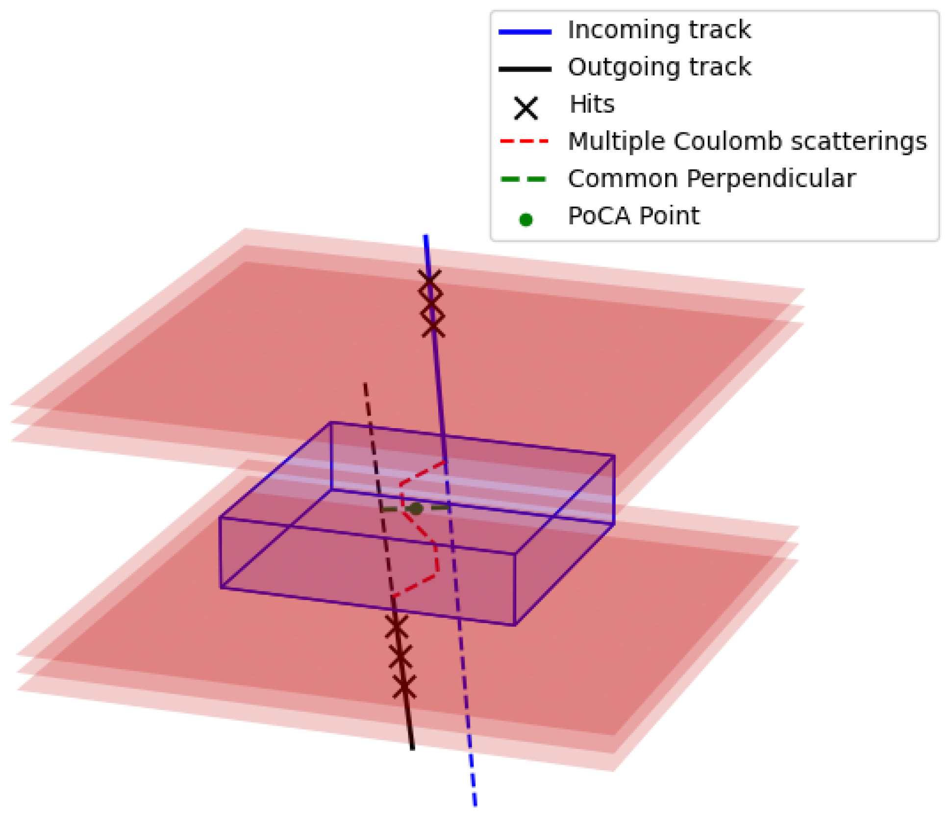
In scattering muon tomography, a very common method for the reconstruction of volumes of interest is the point-of-closest-approach (PoCA) reconstruction [12]. This is achieved by performing, per muon event, separate linear fits on hits recorded above and below the volume of interest, yielding incoming and outgoing muon tracks. The PoCA point is then defined as the closest point between these two tracks in three-dimensional space, represented by the midpoint of the normal segment connecting the two tracks (Figure 2). The point constitutes an approximation of the entirety of the multiple Coulomb scatterings that the muon undergoes as it traverses the volume.
In the context of cargo container imaging for the detection of illicit materials, it is crucial to complement the PoCA reconstruction with an inference of the constituent materials and composition of the volume of interest. This necessitates the employment of a suitable inference algorithm capable of solving the inverse problem by leveraging of the relevant spatial and/or scattering variables of the PoCA points.
In this section, we expand on two volume inference algorithms. The first one is a radiation-length inference method, and the second one is based on a binned clustering algorithm. A recently implemented detector design [13], referred to as the ’hodoscope’, is used as part of our contribution to the SilentBorder project [14]. Instead of optimising individually the position, size and other properties of a set of simple, thin detector panels (Figure 3a), the user can now define a hodoscope as a rigid set of a certain number (three in this study) of detector panels, bound to keeping the same size and relative position, fixed inside a protective casing, as depicted in Figure 3b.
2.1. Inference of Material Radiation Length
The radiation length is estimated in each voxel of the passive volume to infer the dominant material based on the scattering angles of simulated muons. By inverting Equation (1), a radiation length estimator is constructed for this purpose. To simplify the computation, the inversion omits the non-Gaussian natural logarithmic term, which would otherwise require an iterative numerical approach to solve for , increasing computational complexity. High-density materials, such as lead, exhibit lower radiation lengths due to the increased frequency of Coulomb interactions, which arise from the higher concentration of atomic nuclei along the particle’s trajectory. Conversely, low-density materials, such as air, correspond to larger radiation lengths due to the sparsity of atomic nuclei, leading to less frequent interactions.
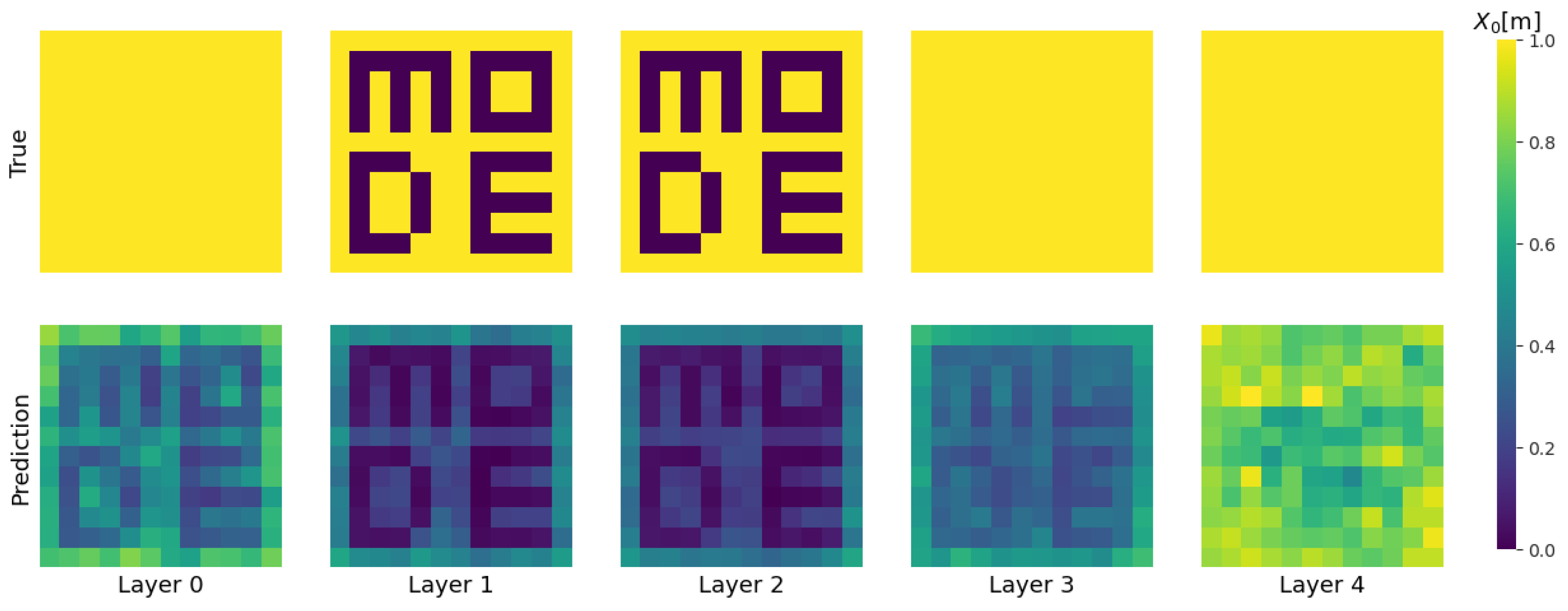
While a more detailed initial study using this algorithm was presented in [13], an illustrative example is provided below. For this example, Figure 4 shows that the reconstructed volume does not fully replicate the original. The accuracy of the reconstruction is influenced by the acceptance and spatial resolution of the detectors and by the number of muons that traverse the passive volume. These factors collectively affect the number of useful reconstructed PoCA points and the precision of their spatial localisation, which directly impacts the accuracy of the estimation.
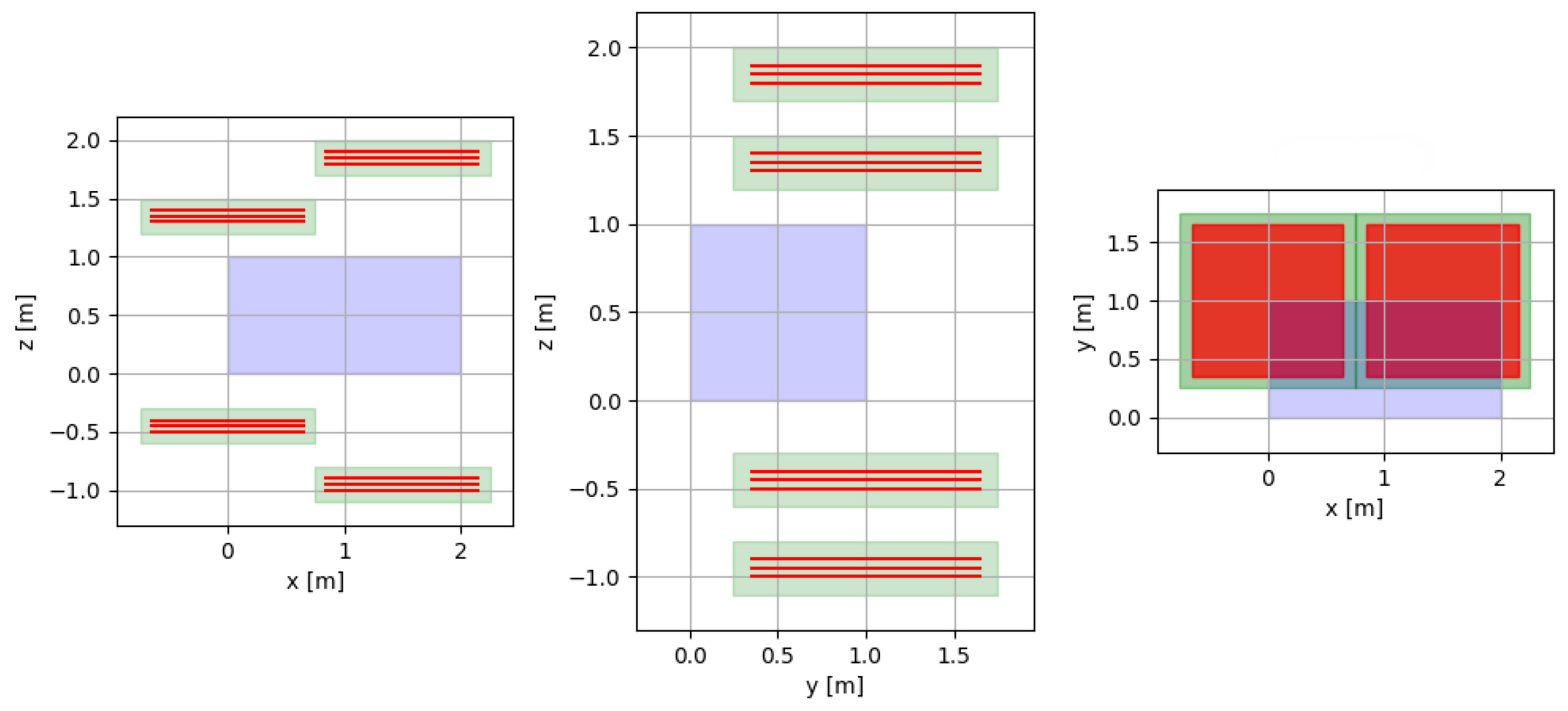
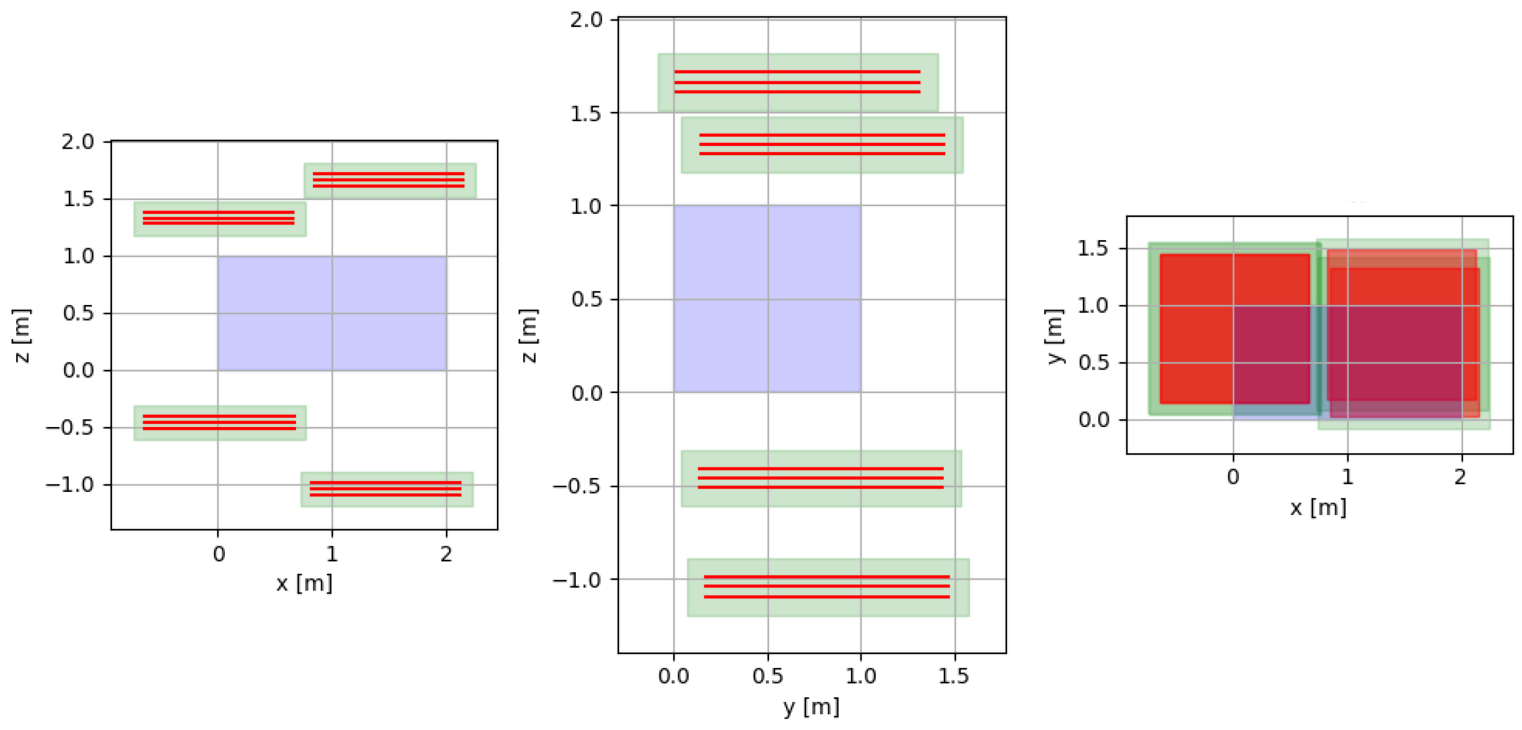
For the optimisation study presented in this section, a system of four hodoscopes, each with dimensions (the quoted dimensions are not the actual dimensions of the hodoscopes but are used for illustrative purposes), is arranged as two pairs placed above and below a passive volume, with a slight gap between each pair, as shown in Figure 5. The optimisation was performed with 15 different material configurations for each passive volume batch per epoch, simulating 8000 muons for each configuration. This number of simulated muons is considered adequate to ensure the proper operation of the algorithm for a volume of this size. After optimisation, although no significant change is observed in the plane, the final configuration in Figure 6 shows that the upper pair of hodoscopes has been moved closer in the z direction.
This radiation-length inference algorithm effectively addresses detector positioning issues, though certain limitations remain. Figure 7 presents the evolution over epochs of the MSE loss, computed between the inferred and ground truth voxel , for the optimisation example discussed previously. During training, the loss decreases by more than an order of magnitude, indicating that the algorithm functions as expected and that the detector configuration is being optimised. However, the training loss exhibits noticeable fluctuations, which are indicative of a bias stemming from the overall underestimation of the radiation length values, as discussed in [13]. This bias must be addressed before optimising more complex detector parameters in non-trivial scenarios, ensuring that the outcome of gradient descent optimisation remains reliable. This issue is currently under investigation for a future publication.
2.2. Binned Clustering Algorithm
Our implementation of a binned clustering algorithm (BCA) as a reconstruction method is built upon the algorithm developed in [15]. It was originally intended for border control applications as an anomaly detection algorithm in a scenario where cargo containers are scanned to obtain a yes/no decision on whether they should be subject to further inspection, within a short time frame (as short as 1 min in [15]). The algorithm aims at quantifying ‘clusteredness’ in a voxelised volume, which is related to the atomic number Z of the material. In traversing volumes of varying density, muons are expected to undergo larger-angle scatterings where denser materials are located. Hence, the algorithm presented in Ref. [15] proceeds as follows: Within each voxel of the scanned volume, scattering vertices are sorted in decreasing order of their scattering angles . A selection of the first of the sorted vertices is taken in order to mitigate any dependence on the number of vertices inside different voxels. For each pair of scattering vertices i and j within this selection, a metric , is defined as the distance between the two vertices. A weighted metric is obtained by dividing by the product of the associated scattering angles , weighted by the normalised muon momenta :
Here, the normalised momentum is defined as:
where it is customary to set , which is approximately the average momentum of cosmic muons at sea level.
The median of the per-voxel distribution of weighted metrics is an indicator of the material density. Denser materials, such as uranium, yield lower median values, as scattering vertices are larger and in closer proximity. On the other hand, low-density materials such as air or light cargo lead to higher median values. Setting the voxel score to be median of , where the natural logarithm serves for a better separation of the otherwise very close values, the final discriminator of the volume as a whole is taken as the minimal value of its voxel score distribution. A threshold for the discriminator is chosen based on the voxel score distributions for volumes of different materials, such that values of the discriminator below a certain threshold indicate the presence of a high-Z-material block, such as uranium.
Based on this algorithm, we build our implementation for TomOpt, which takes in the reconstructed PoCA points as the scattering vertices. For simplicity, considering that most muon tomography setups are not equipped (for reasons of budget or logistics) with means to measure momentum, we simplify Equation (2) by setting all momentum weights to unity.
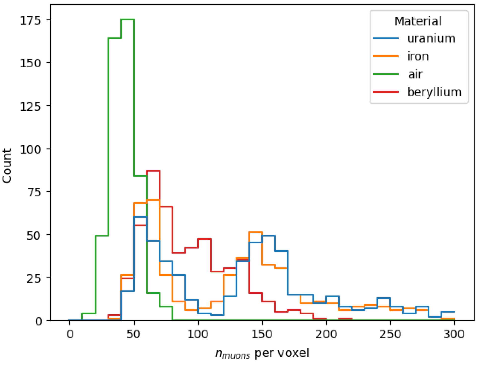
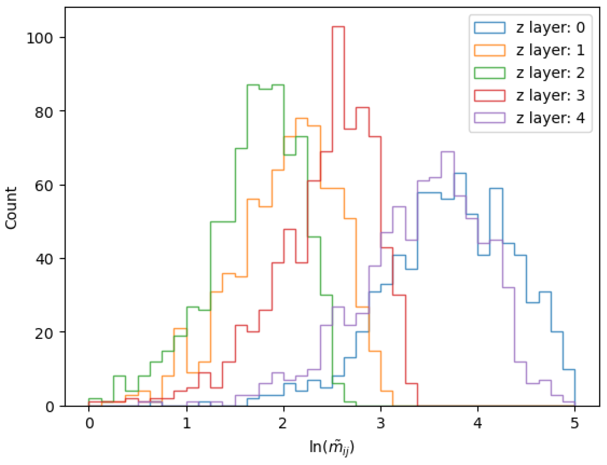
To assess the impact of material type on the estimated voxel score, a simulation is performed using the TomOpt framework in prediction mode, functioning as a volume inference tool without any optimisation. The scan is performed for a homogeneous volume (of a voxel side length) and for different materials of the volume: uranium, iron, beryllium, and air. To ensure all voxels are populated with PoCA points, the number of generated muons is set to 100,000, which is the usable number of muons that pass through the volume. Figure 8 illustrates the number of PoCA points in each voxel of the scanned volume for these four materials. Based on information from this graph, we set the maximum number of PoCA vertices per voxel at .
The voxel score distribution for different materials of the scanned volume (uranium, iron, beryllium, and air) is illustrated in Figure 9. The material classification feature of this algorithm manifests in the separation of the distributions corresponding to different materials, with high-Z materials such as uranium peaking at lower values (below 4), and low-Z materials (beryllium and air) shifted to much higher values. The double-peak splitting of the distributions, in addition to detector acceptance, is an effect of the localisation of large scatterings at the volume centre, which is described below.
In Figure 10, the distribution of the weighted metric () in five voxels of a uranium volume is shown. These voxels are at the same x and y position (indices: ) but are located at different z positions spanning over the height of the volume (). Voxels and are at the bottom and top of the scanned volume, respectively. A shift in the median of the distributions of these two voxels is observed toward larger values compared to the medians of the other distributions. This can be reasoned by the inherent concentration of reconstructed PoCA points at the centre of the scanned volume with fewer vertices of lower scattering angles reconstructed near the edges. This is further demonstrated in Figure 11. The distribution of the factor used to weight the BCA metric is shown in Figure 11a for the aforementioned voxels. It is clearly noticed that values for the edge voxels peak at lower values, while the distribution of the central voxel peaks at the largest value. As Figure 11b does not show any discrepancy for the metric distributions for the same number of selected PoCA vertices in a homogeneous material volume, the splitting effect of the weighted metric distribution can be attributed to the predominance of large scatterings in the centre region of the volume. Although this double-peak structure is an inherent characteristic of the PoCA approach, it does not pose any concern for the present study, as the final discriminator of the distribution is of primary interest, irrespective of its shape. Nonetheless, its analysis was necessary to clarify the origin of the observed peaks and to dispel any potential confusion.
In its last step, the algorithm extracts a final discriminator of the volume which is the minimum value of the distribution of median , allowing for a feasible classification task: the detection of a uranium anomaly within a cargo volume. For this, a suitable threshold value for this discriminator should be chosen, below which the algorithm signals the presence of a uranium block and calls for inspection of the cargo. In the following, we carry out a discrimination task to classify volumes into signal volumes (containing a U block) and background volumes (not containing a U block).
2.2.1. Use-Case Study: Uranium in a Lorry
For this study, the scanned (passive) volume represents a lorry, modeled as a box with a base layer of iron. The interior of the lorry is filled with cubic voxels of side length , randomly assigned materials from a predefined set of “background” materials. In our study, the set of background materials consists of iron, beryllium, and air. The extent to which the lorry is filled is controlled by a fill level parameter ranging from 0 to 1. If the fill fraction is less than 1, the remaining space is assumed to be air. We set this parameter to . Additionally, a “signal” material—uranium (U) in this case—is introduced at a random location within the volume, with an adjustable size (in ) and a probability of presence. A passive volume generator is employed to randomly construct these configurations, referred to as “U-lorry” volumes.
To evaluate the performance of the BCA algorithm in detecting uranium within a U-lorry, two types of passive volumes are generated:
Signal+Background Volume: A configuration containing a uranium block spanning two adjacent voxels.
Background-Only Volume: A configuration with no uranium block
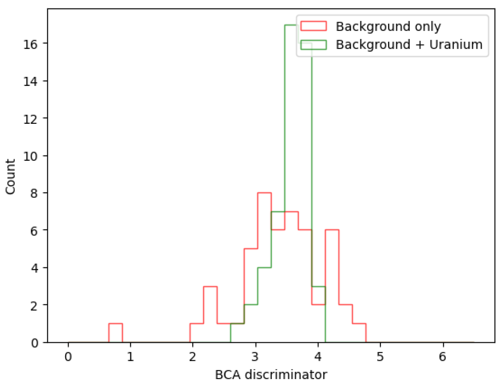
We first assess the classification capability with an optimal detector configuration consisting of two hodoscopes positioned symmetrically above and below the passive volume with their centers aligned with the centre of the passive volume. Each volume is exposed to 100,000 simulated muons. The BCA score distributions for the different materials present in the passive volumes are shown in Figure 12. Although the distribution of iron in Figure 12a overlaps with those of low-Z materials (beryllium and air), the uranium-containing voxels are distinctly separated, with scores isolated below 4. The presence of entries at bin 0 for air corresponds to voxels that received no PoCA vertices and are therefore ignored. The final discriminator for the passive volume, defined as the minimum of the BCA score distribution across all voxels, is expected to be close to 4. This threshold is motivated by Figure 12b, which illustrates the background-only case where all discriminator values exceed 4.
In order to obtain a statistical assessment of the discriminator threshold, two sets of passive volumes are generated. The first set consists of 50 signal + background volumes containing a randomly positioned uranium block, and the second set consists of 50 background-only passive volumes. The final discriminator for each volume’s BCA score distribution is extracted. The different discriminators of the volumes of both sets are plotted in Figure 13.
The perfect discrimination between the two sets of passive volumes suggests incorporating the BCA discriminator into the loss function definition for the TomOpt optimisation step. Given the binary nature of this classification task, the discriminator is passed through a reversed sigmoid activation function to map it to values between 0 and 1. The sigmoid function is centered at 3.5, motivated by the observed value of the discriminator threshold (Figure 12b). The loss function can therefore be thought of as the binary cross-entropy (BCE) between the true classes (0 or 1) and the sigmoid-transformed discriminator. Given the large number of muons involved, the computation time per passive volume is on the order of a few minutes. This means that for training/optimisation, we are constrained to using a smaller number of passive volumes per epoch. For the optimisation study described below, the passive volume batch per epoch consists of ten U-lorry passive volumes equally divided into background-only and signal+background volumes, and the number of muons passed through each passive volume is . The optimisation starts with an initial detector configuration of two hodoscopes (each of a size of ) placed above and below the scanned passive volume whose center is at (Figure 14). The bottom hodoscope has its center (in ) aligned with that of the passive volume, whereas the upper hodoscope is shifted such that its center is at . The optimisation is performed over 20 epochs.
2.2.2. Optimisation Results
It is expected after an optimal optimisation process to have the upper hodoscope’s position progressively shifted to align it with the passive volume while having a progressively decreasing loss function over several epochs. In Figure 15, we observe that the overall BCE loss decreases over the 20 epochs. However, this loss function does decrease smoothly, and we observe sharp fluctuations throughout the optimisation epochs. These fluctuations, which are significantly larger during the first half of the optimisation process, are primarily due to the imperfect inference of smaller discriminator values for background volumes, which are incorrectly classified as signal volumes, thereby increasing the loss. In contrast, the signal volumes tend to be correctly classified and decrease the loss. This is seen in Figure 16 showing the discriminator predictions for 100 passive volumes divided into background and signal+background volumes, where the initial off-centered configuration of hodoscopes described above is used. The false positives observed arise from the incorrect inference of background volumes. Specifically, muons traversing regions of the passives that are not covered by the upper detector experience high uncertainties in their recorded positions due to our differentiable modeling of detector efficiency and resolution. This leads to an overestimation of scattering angles in these regions, ultimately resulting in an underestimation of the BCA discriminator. Additional details on this effect are provided in Appendix A, which presents a complementary optimisation study using a simplified passive volume.
Figure 17 presents the final optimised detector configuration, which shows a shift in the position of the upper hodoscope, now providing improved coverage of the passive volume. To assess the enhancement in performance following optimisation, we conduct a classification test comparing the pre- and post-optimisation configurations using standard performance metrics.
For this evaluation, we generate a batch of 20 random U-lorry volumes: 10 containing uranium and 10 background volumes. Each volume undergoes inference using TomOpt in volume prediction mode (i.e., without optimisation of detector parameters).
Figure 18 displays the confusion matrices for both configurations. In the pre-optimisation configuration, the model trivially predicts all volumes as positive, resulting in perfect true positive (TP) identification but complete misclassification of negative cases as false positives (FPs). In contrast, the optimised configuration achieves perfect classification for both true positive and true negative (TN) cases, eliminating false positives.
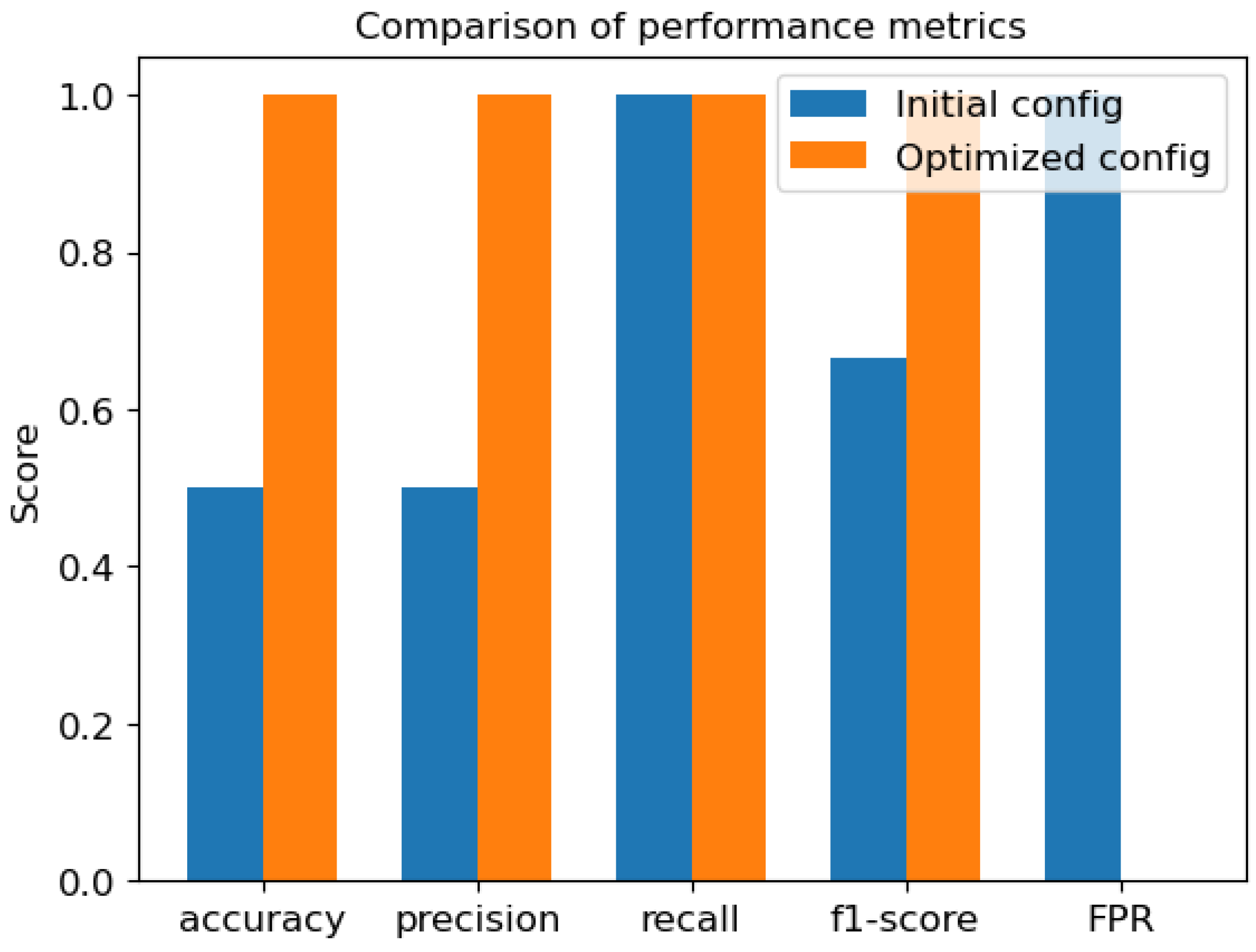
Figure 19 compares key performance metrics, highlighting the substantial improvement in classification power achieved through the optimisation process.
These metrics are calculated as follows:
Accuracy measures the proportion of correct predictions (both true positives and true negatives) out of all predictions. It is defined as:
where is the number of true positives, is the number of true negatives, is the number of false positives, and is the number of false negatives. A higher accuracy indicates a better overall performance of the classifier.
Precision, also known as positive predictive value, measures the proportion of positive predictions that are actually correct. It is defined as:
Precision is important when the cost of false positives is high and we want to minimise the number of incorrect positive classifications.
Recall, or sensitivity, measures the proportion of actual positive cases that are correctly identified by the classifier. It is defined as:
Recall is critical when we want to minimise false negatives and ensure that as many true positive cases as possible are detected.
The F1-score is the harmonic mean of precision and recall, providing a single measure that balances both metrics. It is defined as:
The false positive rate measures the proportion of actual negatives that are incorrectly classified as positive. It is defined as:
A lower FPR is desirable, as it indicates that the classifier is less likely to misclassify negative cases as positive.
The results in Figure 19 demonstrate the substantial improvement in classification performance after optimisation, particularly in precision, accuracy, and F1-score, while maintaining perfect recall in both configurations. The perfect recall of the initial configuration is due to the correct classification of true positives in the absence of false negatives. Additionally, the FPR is reduced to 0 for the post-optimisation configuration, being initially 1.
3. Discussion and Conclusions
In this work, we have presented an initial implementation of a binned clustering algorithm for volume inference within the TomOpt optimisation pipeline. The TomOpt differential detector modeling propagates resolution and efficiency uncertainties to the reconstructed detector hits, which in turn affect the PoCA variables used in the BCA computations. Consequently, the resulting BCA discriminator, an input to the loss function for gradient descent, is sensitive to the detector geometry as intended. To further improve the BCA computations, it is necessary to account for the uncertainties on the PoCA variables. This can be achieved by reformulating the BCA algorithm to utilise Gaussian probability distributions for the PoCA points, which extend over the entire scanned volume. This approach allows for weighting the calculations in each voxel of the volume by considering the entire PoCA population, rather than relying on a sharp selection from the population. This eliminates the need for a large number of sampled muons.
Due to the inverse relationship between the BCA score and material density, an approximate linear correlation can be established with the material radiation length . This observation suggests the incorporation of a mean-error-type loss function that evaluates the difference error between the voxel BCA scores and their corresponding reference values.
To maintain a controlled and interpretable study, a limited set of free parameters has been chosen—the positions—while keeping the inner panels’ dimensions and separations fixed. This enabled us to assess the behaviour of gradient descent in a well-defined and simplified optimisation scenario, where the expected optimal configuration is predetermined. Ongoing work aims to extend the optimisation beyond simple parameters by incorporating more complex detector design variables, such as panel spacing in the z-direction within the hodoscope and the gap size between adjacent hodoscopes. These additions will contribute to determining a fully optimised configuration.
This is currently a work in progress.
Author Contributions
Funding acquisition, A.G.; Methodology, Z.Z., M.L. and P.V.; Project administration, A.G.; Software, S.A., M.L., G.C.S. and P.V.; Supervision, A.G.; Visualisation, Z.Z. and S.A.; Writing—original draft, Z.Z. and S.A.; Writing—review and editing, T.D., A.G., M.L., P.V. and H.Z. All authors have read and agreed to the published version of the manuscript.
Funding
The authors acknowledge funding from the EU Horizon 2020 Research and Innovation Programme under grant agreement no. 101021812 (“SilentBorder”) and by the Fonds de la Recherche Scientifique—FNRS under Grants No. T.0099.19 and J.0070.21. Pietro Vischia’s work was supported by the “Ramón y Cajal” program under Project No. RYC2021-033305-I funded by the MCIN MCIN/AEI/10.13039/501100011033 and by the European Union NextGenerationEU/PRTR.
Computational resources have been provided by the supercomputing facilities of the Université catholique de Louvain (CISM/UCL) and the Consortium des Équipements de Calcul Intensif en Fédération Wallonie Bruxelles (CÉCI) funded by the Fond de la Recherche Scientifique de Belgique (F.R.S.-FNRS) under convention 2.5020.11 and by the Walloon Region. The authors wish to thank the members of Work Package 3 of the SilentBorder project, and in particular Vitaly Kudryavtsev, for several insightful discussions. Finally, the authors gratefully acknowledge the computer resources at Artemisa, funded by the European Union ERDF and Comunitat Valenciana as well as the technical support provided by the Instituto de Fisica Corpuscular, IFIC (CSICUV).
Conflicts of Interest
The authors declare no conflicts of interest.
Correction Statement
This article has been republished with a minor correction to the Acknowledgments Statement. This change does not affect the scientific content of the article.
Appendix A. Complementary Optimisation Study with a Simplified Passive Volume
In this complementary optimisation study, instead of the randomly generated U-lorry volumes, we choose much simpler passive volumes. Background-only volumes consist entirely of beryllium, and signal+background volumes contain a uranium block placed at the corner near and halfway in the z-direction (Figure A1). The detectors are again two hodoscopes placed above and below the volume. We study the optimisation of two initial hodoscope configurations, referred to as Case A and Case B:
Case A: the upper hodoscope initially centered at (on the opposite side of the uranium block);
Case B: the upper hodoscope initially centered at (above the uranium block).
The optimisation cycle is performed over 20 epochs. In each epoch, 100,000 muons are passed through a batch consisting of two passive volumes. For Case A, the batch consists of a background-only beryllium volume and a signal+background volume. For Case B, the volume batch includes two signal+background volumes. Following PoCA reconstruction, BCA inference is carried out for each of these volumes to extract the final discriminator, which is then used in the loss function calculations.
In Figure A2, the loss curve for Case A is shown. While a general decrease in loss is observed, the loss exhibits significant sharp fluctuations and does not reach a stable minimum. The false positives observed in Figure A3 result from the incorrect inference of the background volumes, where muons traversing the region of the passives not covered by the upper detector receive high uncertainties on their recorded positions in the detectors according to our differentiable detector modeling of efficiency and resolution. This leads to an overestimation of scattering angles in this region, which results in an underestimation of the BCA discriminator (Figure A4). On the other hand, the signal distribution extends toward higher BCA discriminator values compared to Figure 16. This aligns with our prior observations: in Case A, the uranium block is initially positioned in a corner () that is not covered by the upper hodoscope, and in the final configuration, this region remains uncovered. As a result, some PoCA points corresponding to large scatterings inside the uranium block are reconstructed elsewhere in the lighter beryllium background due to the uncertainty on the recorded hit positions above the uranium block. The final detector position, shown in Figure A5, reveals a shift in the upper hodoscope towards a larger coverage of the passive volume, suggesting that the optimisation process is progressing in a meaningful direction. However, the fluctuations in the loss function indicate that it remains highly noisy and not sufficiently sensitive to small positional shifts. A similar behavior is observed in Case B, as shown in Figure A6, although the overall loss is approximately four orders of magnitude smaller. This comes from the fact that only signal volumes are inferred. However, the position of the upper hodoscope in this case shows almost no change at the end of the optimisation, as depicted in Figure A5, which is an expected behaviour since it fully covers the uranium block in this case. The sensitivity of the current loss function to noise motivates the exploration of an alternative loss formulation based on image reconstruction. Such a loss would offer more stable gradient updates and provide better control during the optimisation, which is particularly important for ensuring the convergence of gradient descent when optimising more complex detector design parameters.
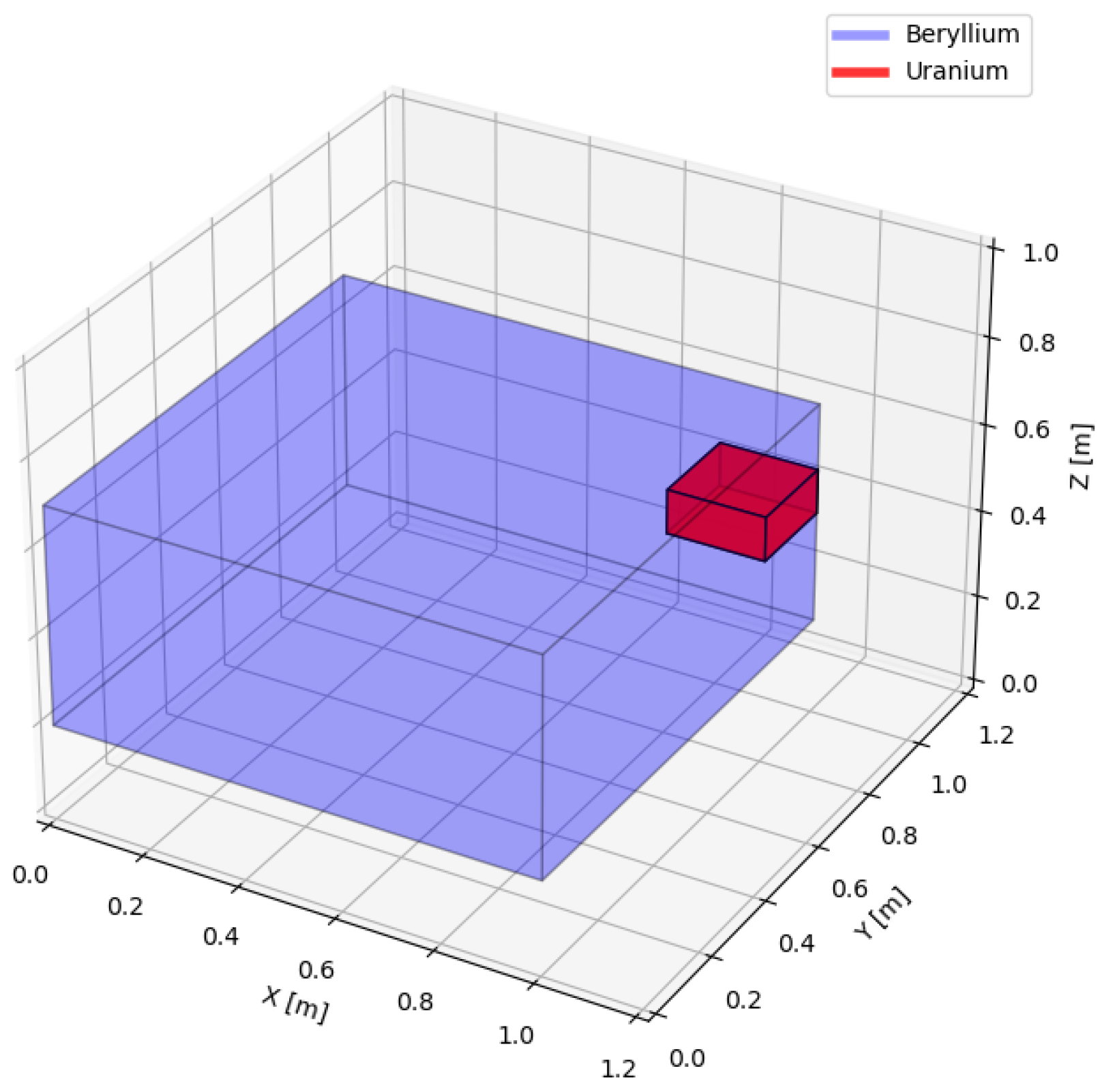
Figure A1.
A simplified passive volume made up of beryllium (background material). For signal+background volumes, a uranium block is inserted at the voxel position .
Figure A1.
A simplified passive volume made up of beryllium (background material). For signal+background volumes, a uranium block is inserted at the voxel position .
Figure A2.
Summary of the BCE loss over 20 epochs of the optimisation cycle. Simplified passive volumes and the initial detector configuration of Case A are used. Epochs 0–5 are warm-up epochs.
Figure A2.
Summary of the BCE loss over 20 epochs of the optimisation cycle. Simplified passive volumes and the initial detector configuration of Case A are used. Epochs 0–5 are warm-up epochs.
Figure A3.
BCA discriminators of background Be volumes (red) and of signal volumes (green) containing a uranium block placed at the corner near and halfway in the z-direction. The final post-optimisation configuration of Case A is used for these predictions. Compared to Figure 16, the signal distribution extends toward higher BCA discriminator values. This is due to the uncertainty on the recorded hit positions above the uranium block, which remains uncovered by the upper hodoscope, causing some PoCA points corresponding to large scatterings inside the uranium block to be reconstructed elsewhere in the lighter beryllium background.
Figure A4.
Overlay of the scattering angles weighting factor () distributions inside voxels of indices () in a background-only beryllium volume computed for a shifted upper hodoscope at (a) compared to that obtained with a reference configuration having the upper hodoscope centred at (b).
Figure A4.
Overlay of the scattering angles weighting factor () distributions inside voxels of indices () in a background-only beryllium volume computed for a shifted upper hodoscope at (a) compared to that obtained with a reference configuration having the upper hodoscope centred at (b).
Figure A5.
Final detector positions in for Case A (left) and Case B (right). The first and second rows correspond to the upper and lower hodoscopes, respectively. Hodoscopes are represented by blue squares, passive volumes by black squares, and muon generation surfaces by green meshed squares.
Figure A5.
Final detector positions in for Case A (left) and Case B (right). The first and second rows correspond to the upper and lower hodoscopes, respectively. Hodoscopes are represented by blue squares, passive volumes by black squares, and muon generation surfaces by green meshed squares.
Figure A6.
Summary of the BCE loss over 20 epochs of the optimisation cycle. Simplified passive volumes and the initial detector configuration of Case B are used. Epochs 0–5 are warm-up epochs.
Figure A6.
Summary of the BCE loss over 20 epochs of the optimisation cycle. Simplified passive volumes and the initial detector configuration of Case B are used. Epochs 0–5 are warm-up epochs.
Bonechi, L.; D’Alessandro, R.; Giammanco, A. Atmospheric muons as an imaging tool. Rev. Phys.2020, 5, 100038. [Google Scholar] [CrossRef]
International Atomic Energy Agency. Muon imaging: Present Status and Emerging Applications; IAEA TECDOC 2012; IAEA: Vienna, Austria, 2022. [Google Scholar]
Barnes, S.; Georgadze, A.; Giammanco, A.; Kiisk, M.; Kudryavtsev, V.A.; Lagrange, M.; Pinto, O.L. Cosmic-Ray Tomography for Border Security. Instruments2023, 7, 13. [Google Scholar] [CrossRef]
Rutherford, E. The scattering of α and β particles by matter and the structure of the atom. Lond. Edinb. Dubl. Phil. Mag.1911, 21, 669. [Google Scholar] [CrossRef]
Strong, G.C.; Lagrange, M.; Orio, A.; Bordignon, A.; Bury, F.; Dorigo, T.; Giammanco, A.; Heikal, M.; Kieseler, J.; Lamparth, M.; et al. TomOpt: Differential optimisation for task- and constraint-aware design of particle detectors in the context of muon tomography. Mach. Learn. Sci. Technol.2024, 5, 035002. [Google Scholar] [CrossRef]
Strong, G.C.; Bordignon, A.; Dorigo, T.; Fanzago, F.; Giammanco, A.; Kieseler, J.; Lamparth, M.; Lagrange, M.; Martínez Ruíz del Árbol, P.; Nardi, F.; et al. TomOpt: Differential Muon Tomography Optimisation. 2024. Available online: https://github.com/GilesStrong/tomopt (accessed on 25 April 2025).
Paszke, A. PyTorch: An Imperative Style, High-Performance Deep Learning Library. In Advances in Neural Information Processing Systems 32; Curran Associates, Inc.: Red Hook, NY, USA, 2019; p. 8024. [Google Scholar]
Guan, M.; Chu, M.C.; Cao, J.; Luk, K.B.; Yang, C. A parametrization of the cosmic-ray muon flux at sea-level. arXiv2015, arXiv:1509.06176. [Google Scholar]
Shukla, P.; Sankrith, S. Energy and angular distributions of atmospheric muons at the Earth. arXiv2018, arXiv:1606.06907. [Google Scholar] [CrossRef]
Hoch, R.; Mitra, D.; Gnanvo, K.; Hohlmann, M. Muon Tomography Algorithms for Nuclear Threat Detection; Springer Nature: Berlin/Heidelberg, Germany, 2009; Volume 214, p. 225. [Google Scholar]
Zaher, Z.; Lagrange, M.; Alvarez, S.; Strong, G.C.; Bury, F.; Giammanco, A.; Dorigo, T.; Orio, A.; Vischia, P.; Zaraket, H. Optimisation of muon portals for border controls using TomOpt. In Proceedings of the MARESEC 2024, Bremerhaven, Germany, 6–7 June 2024. [Google Scholar] [CrossRef]
Georgadze, A.; Giammanco, A.; Kudryavtsev, V.; Lagrange, M.; Turkoglu, C. A Simulation of a Cosmic Ray Tomography Scanner for Trucks and Shipping Containers. J. Adv. Instrum. Sci.2024, 1. [Google Scholar] [CrossRef]
Thomay, C.; Velthuis, J.J.; Baesso, P.; Cussans, D.; Morris, P.A.W.; Steer, C.; Burns, J.; Quillin, S.; Stapleton, M. A binned clustering algorithm to detect high-Z material using cosmic muons. JINST2013, 8, P10013. [Google Scholar] [CrossRef]
Figure 1.
A schematic of the TomOpt optimisation pipleine, reproduced from [7].
Figure 1.
A schematic of the TomOpt optimisation pipleine, reproduced from [7].
Figure 2.
A schematic of the PoCA algorithm. Incoming and outgoing tracks are fitted using muon hits in the upper and lower panels. The estimated scattering vertex, which corresponds to the closest point between these two fitted tracks in 3D, is given by the midpoint of the common perpendicular to the two tracks. This point approximates the multiple Coulomb scatterings inside the volume of interest.
Figure 3.
Several simple detector panels (red) placed above and below a passive volume (blue) (a). Hodoscopes (green) consisting of three detector panels (red) (b).
Figure 3.
Several simple detector panels (red) placed above and below a passive volume (blue) (a). Hodoscopes (green) consisting of three detector panels (red) (b).
Figure 4.
Radiation length inference example of a passive volume made of aluminium and containing an arrangement of lead blocks forming the word ‘MODE’. The first (second) row shows cross-sectional heatmaps along the z direction of the normalised true (inferred) values of voxel-wise . The cross-sections, ordered from left to right, span from the bottom (Layer 0) to the top (Layer 4) of the volume. The shortcoming of reconstruction algorithms and the spatial resolution of the detection system cause the blurring of the reconstructed image across the z direction.
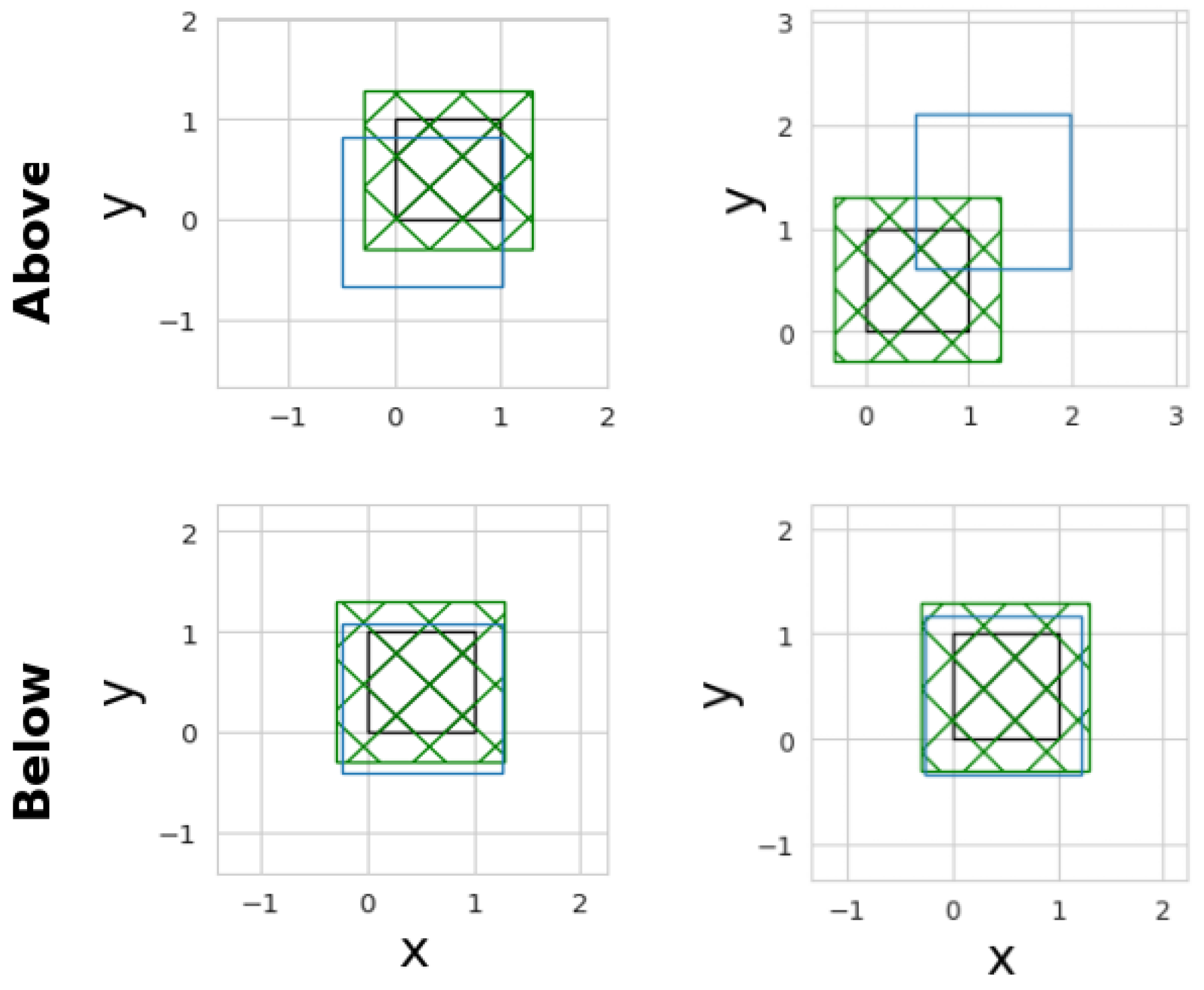
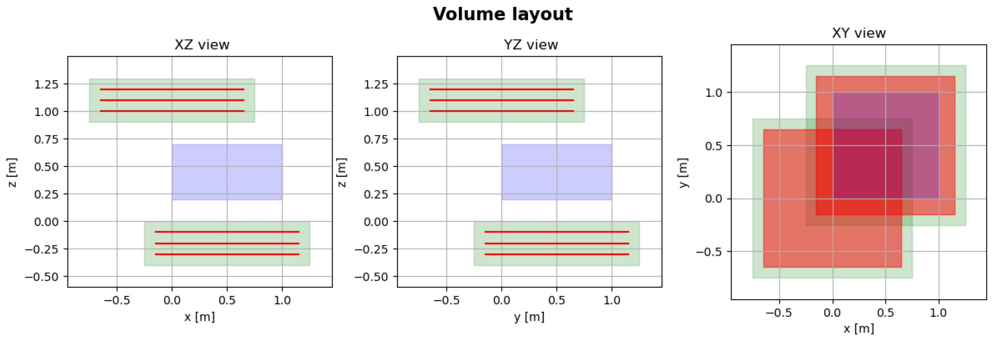
Figure 5.
Initial system configuration, showing the XZ (left), YZ (middle), and XY (right) 2D projections. Hodoscopes are shown in green, inner detector panels in red, and the passive volume in violet.
Figure 5.
Initial system configuration, showing the XZ (left), YZ (middle), and XY (right) 2D projections. Hodoscopes are shown in green, inner detector panels in red, and the passive volume in violet.
Figure 6.
Post-optimisation system configuration, showing the XZ (left), YZ (middle), and XY (right) 2D projections. Hodoscopes are shown in green, inner detector panels in red, and the passive volume in violet.
Figure 6.
Post-optimisation system configuration, showing the XZ (left), YZ (middle), and XY (right) 2D projections. Hodoscopes are shown in green, inner detector panels in red, and the passive volume in violet.
Figure 7.
MSE loss function for the optimisation cycle described in Section 2.1. The vertical axis is shown in a log scale.
Figure 7.
MSE loss function for the optimisation cycle described in Section 2.1. The vertical axis is shown in a log scale.
Figure 8.
An overlay of the distribution of the number of PoCA vertices in voxels filled with different materials. This distribution is limited to smaller values for low-Z materials (air) compared to a wider range for denser materials. By selecting the maximum number of PoCA vertices in all voxels to be 40, the dependence of the BCA voxel score on the number of muons can be reduced, keeping the dependence on the material density.
Figure 9.
BCA voxel score distributions for different materials in the scanned volume. A voxel score is the median of the per-voxel distribution of .
Figure 9.
BCA voxel score distributions for different materials in the scanned volume. A voxel score is the median of the per-voxel distribution of .
Figure 10.
The distribution of the BCA weighted metric in five voxels of a uranium volume. These voxels are at the same x and y position (indices: ) but are located at different z positions spanning over the height of the volume (), which translates to different weighted metric values.
Figure 10.
The distribution of the BCA weighted metric in five voxels of a uranium volume. These voxels are at the same x and y position (indices: ) but are located at different z positions spanning over the height of the volume (), which translates to different weighted metric values.
Figure 11.
Distributions of (a) the product of the selected PoCA vertices’ scattering angles, i.e., the weighting factor () of and (b) the distance between the PoCA vertices . The distributions are in five voxels of a uranium volume. These voxels have the same x and y positions (indices: ) but are located at different z positions spanning over the height of the volume ().
Figure 12.
BCA voxel score distributions for the U-lorry signal+background (a) and background-only (b) volumes. Entries in bin 0 corresponding to air in (a) correspond to voxels that did not receive any PoCA vertices and are excluded.
Figure 12.
BCA voxel score distributions for the U-lorry signal+background (a) and background-only (b) volumes. Entries in bin 0 corresponding to air in (a) correspond to voxels that did not receive any PoCA vertices and are excluded.
Figure 13.
Final BCA discriminators of passive volumes composed of only background materials, iron, beryllium, and air (red), and of signal+background volumes containing a randomly placed uranium block (green). The two distributions are clearly separated, which implies a perfect classification. Based on this result, a value of 3.5 is chosen for the discriminator threshold.
Figure 14.
Initial detector configuration in XZ (left), YZ (center), and XY (right) views. Hodoscopes are shown in green, inner detector panels in red, and the passive volume in violet.
Figure 14.
Initial detector configuration in XZ (left), YZ (center), and XY (right) views. Hodoscopes are shown in green, inner detector panels in red, and the passive volume in violet.
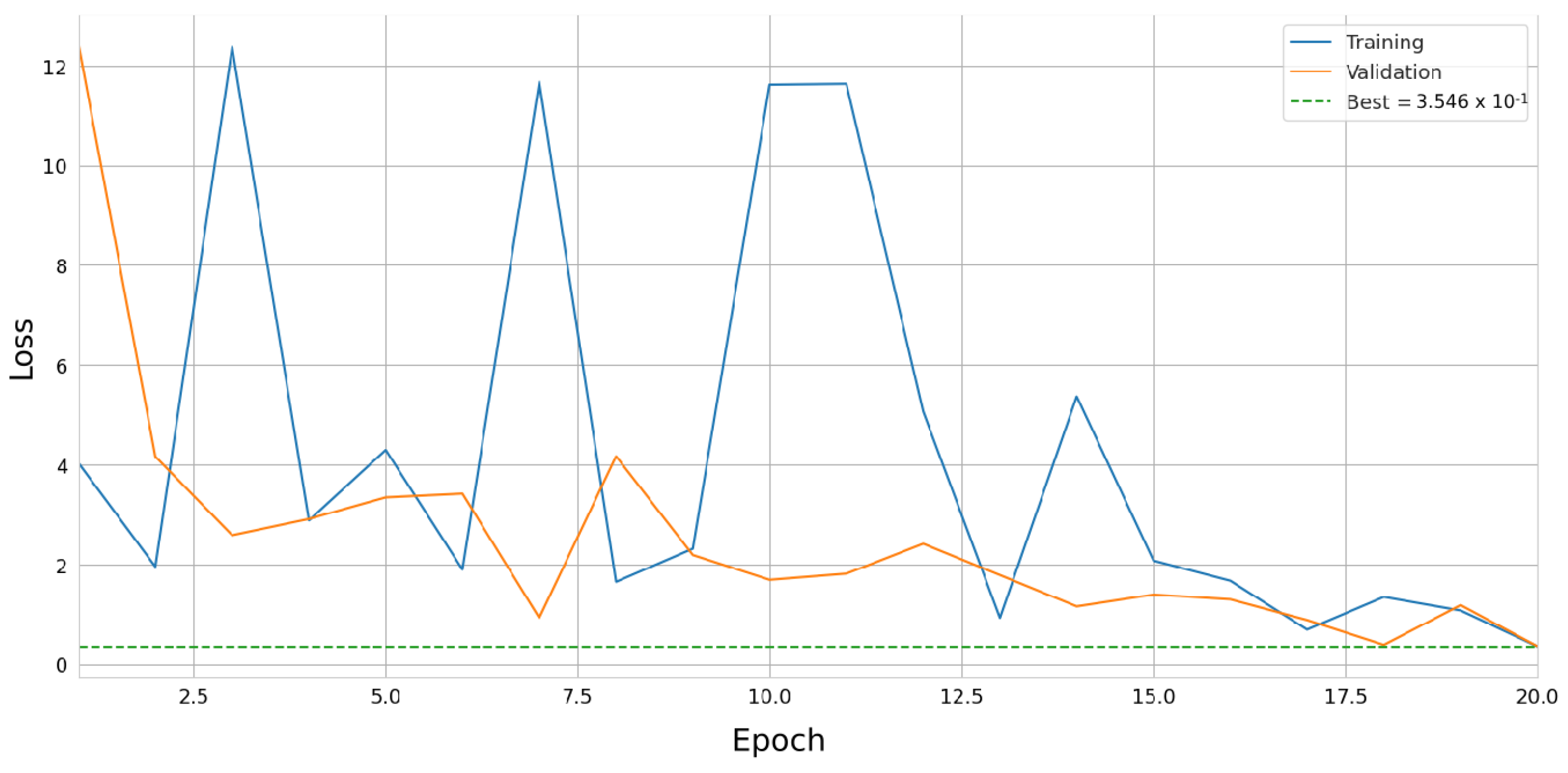
Figure 15.
Summary of the BCE loss over 20 epochs of the optimisation cycle. Passive volumes are randomly generated U-lorry volumes. Epochs 0–5 are warm-up epochs.
Figure 15.
Summary of the BCE loss over 20 epochs of the optimisation cycle. Passive volumes are randomly generated U-lorry volumes. Epochs 0–5 are warm-up epochs.
Figure 16.
BCA discriminators of background volumes (red) and of signal volumes containing a randomly placed uranium block (green). The detectors used for these predictions are two hodoscopes placed above and below the passive volumes, with the above one shifted to only cover a corner of the volumes. An overlap is observed between the two distributions, where signal volumes retain their correct discriminator prediction, whereas background volumes are incorrectly predicted.
Figure 17.
Optimised detector configuration in XZ (left), YZ (center), and XY (right) views. Hodoscopes are shown in green, inner detector panels in red, and the passive volume in violet.
Figure 17.
Optimised detector configuration in XZ (left), YZ (center), and XY (right) views. Hodoscopes are shown in green, inner detector panels in red, and the passive volume in violet.
Figure 18.
Confusion matrices summarising the classification performance of the initial (a) and optimised (b) detector configurations by comparing predicted vs. true labels of the inferred passive volumes.
Figure 18.
Confusion matrices summarising the classification performance of the initial (a) and optimised (b) detector configurations by comparing predicted vs. true labels of the inferred passive volumes.
Figure 19.
Comparison of classification performance metrics of the initial and optimised detector configurations.
Figure 19.
Comparison of classification performance metrics of the initial and optimised detector configurations.
Disclaimer/Publisher’s Note: The statements, opinions and data contained in all publications are solely those of the individual author(s) and contributor(s) and not of MDPI and/or the editor(s). MDPI and/or the editor(s) disclaim responsibility for any injury to people or property resulting from any ideas, methods, instructions or products referred to in the content.
Zaher, Z.; Alvarez, S.; Dorigo, T.; Giammanco, A.; Lagrange, M.; Strong, G.C.; Vischia, P.; Zaraket, H.
Optimisation of Muon Tomography Scanners for Border Control Using TomOpt. Particles2025, 8, 53.
https://doi.org/10.3390/particles8020053
AMA Style
Zaher Z, Alvarez S, Dorigo T, Giammanco A, Lagrange M, Strong GC, Vischia P, Zaraket H.
Optimisation of Muon Tomography Scanners for Border Control Using TomOpt. Particles. 2025; 8(2):53.
https://doi.org/10.3390/particles8020053
Chicago/Turabian Style
Zaher, Zahraa, Samuel Alvarez, Tommaso Dorigo, Andrea Giammanco, Maxime Lagrange, Giles C. Strong, Pietro Vischia, and Haitham Zaraket.
2025. "Optimisation of Muon Tomography Scanners for Border Control Using TomOpt" Particles 8, no. 2: 53.
https://doi.org/10.3390/particles8020053
APA Style
Zaher, Z., Alvarez, S., Dorigo, T., Giammanco, A., Lagrange, M., Strong, G. C., Vischia, P., & Zaraket, H.
(2025). Optimisation of Muon Tomography Scanners for Border Control Using TomOpt. Particles, 8(2), 53.
https://doi.org/10.3390/particles8020053
Article Metrics
No
No
Article Access Statistics
For more information on the journal statistics, click here.
Multiple requests from the same IP address are counted as one view.
Zaher, Z.; Alvarez, S.; Dorigo, T.; Giammanco, A.; Lagrange, M.; Strong, G.C.; Vischia, P.; Zaraket, H.
Optimisation of Muon Tomography Scanners for Border Control Using TomOpt. Particles2025, 8, 53.
https://doi.org/10.3390/particles8020053
AMA Style
Zaher Z, Alvarez S, Dorigo T, Giammanco A, Lagrange M, Strong GC, Vischia P, Zaraket H.
Optimisation of Muon Tomography Scanners for Border Control Using TomOpt. Particles. 2025; 8(2):53.
https://doi.org/10.3390/particles8020053
Chicago/Turabian Style
Zaher, Zahraa, Samuel Alvarez, Tommaso Dorigo, Andrea Giammanco, Maxime Lagrange, Giles C. Strong, Pietro Vischia, and Haitham Zaraket.
2025. "Optimisation of Muon Tomography Scanners for Border Control Using TomOpt" Particles 8, no. 2: 53.
https://doi.org/10.3390/particles8020053
APA Style
Zaher, Z., Alvarez, S., Dorigo, T., Giammanco, A., Lagrange, M., Strong, G. C., Vischia, P., & Zaraket, H.
(2025). Optimisation of Muon Tomography Scanners for Border Control Using TomOpt. Particles, 8(2), 53.
https://doi.org/10.3390/particles8020053


 ,
, 