Improved Equations of the Lagrange Top and Examples of Analytical Solutions

Abstract

Equations of a heavy rotating body with one fixed point can be deduced starting from a variational problem with holonomic constraints. When applying this formalism to the particular case of a Lagrange top, in the formulation with a diagonal inertia tensor the potential energy has a more complicated form as compared with that assumed in the literature on dynamics of a rigid body. This implies the corresponding improvements in equations of motion. Therefore, we revised this case, presenting several examples of analytical solutions to the improved equations. The case of precession without nutation has a surprisingly rich relationship between the rotation and precession rates, which is discussed in detail.

1. Introduction

Recent work [1] was devoted to a systematic exposition of the dynamics of a free rigid body, considered as a system with holonomic (velocity-independent) constraints. The constraints in the action functional have been taken into account with the use of Lagrangian multipliers. Having accepted this expression, we no longer need any additional postulates or assumptions about the behaviour of the rigid body. As was shown in [1], all the basic quantities and characteristics of a rigid body, as well as the equations of motion and integrals of motion, are obtained from the variational problem by direct and unequivocal calculations within the framework of standard methods of classical mechanics applied in the laboratory system. Here we follow the same scheme to deduce equations of motion of a rigid body with a fixed point in the gravity field. The analysis is similar to that presented in Sections 2–4 of [1], so we only outline it in Section 2 and Section 3 below, without going into the details.

Then we concentrate on the case of a Lagrange top. This is an axially symmetric heavy body with one point of an axial axis fixed. To be specific, imagine a conical top whose point of base is fixed in space. The Lagrange top is one of the oldest problems of mathematical physics, which has always been considered as the classical example of the integrable system according to Liouville which, moreover, admits a relatively simple qualitative description on the base of effective potential [2,3,4,5,6,7,8,9,10]. However, when formulating its variational problem with the diagonal inertia tensor, we observed that potential energy has a more complicated form as compared with that assumed in the literature on dynamics of a rigid body. This implies the corresponding improvements in equations of motion. Because this is a somewhat surprising observation, its validity and comparison with the literature are carried out in detail at the end of Section II and in Section IV. Being one of the classical problems of nonlinear dynamics and integrable systems, this issue, however, is of interest in the modern studies related with construction and behaviour of spinning particles and rotating bodies in external fields beyond the pole-dipole approximation [11,12,13,14,15,16,17,18,19].

Using Liouville’s theorem, integration of improved equations can be reduced to the calculation of four elliptic integrals [20]. Of course, the answer in the form of elliptic integrals is not very illuminating. Therefore, in Section 5, Section 6, Section 7 and Section 8, we present several examples of solutions to the improved equations in terms of elementary functions: sleeping top, horizontally precessing top, as well as the inclined top precessing without nutation. For the latter case, the solution turned out to be two-frequency motion with a surprising reach relationship between the frequencies; that, besides the inclination, depends also on the top’s geometry. We also discussed the case of an awakened top, for which there is no longer a solution in elementary functions. The qualitative and numerical analysis of this case is based on the study of effective potential.

2. Rigid Body with a Fixed Point

In this section we confirm that equations of motion for the rotational degrees of freedom of a rigid body with a fixed point formally coincide with those of a free rigid body (see Equation (10) below). The only difference is that all quantities, including the inertia tensor, its eigenvalues, and eigenvectors, should be calculated in the laboratory system with the origin in the fixed point instead of the centre of mass.

We use the notation adopted in [1]. In particular, the notation for the scalar product is $(\mathbf{a},\mathbf{b})=a_i{b}_i$. Notation for the vector product is ${[\mathbf{a},\mathbf{b}]}_i={ϵ}_{ijk}{a}_j{b}_k$, where ${ϵ}_{ijk}$ is the Levi-Chivita symbol in three dimensions, with ${ϵ}_{123}=+1$.

A rigid body is considered as a system, composed of n points with the coordinates $y_N^i$, and masses $m_N$, $N=1,2,\dots ,n,i=1,2,3$. To the constraints $({\mathbf{y}}_N\left(t\right)-{\mathbf{y}}_K\left(t\right),{\mathbf{y}}_P\left(t\right)-{\mathbf{y}}_M\left(t\right))=\mathrm{const}$, determining a free rigid body, we add more constraints: $|{\mathbf{y}}_N\left(t\right)-{\mathbf{y}}_0|=\mathrm{const}$, where ${\mathbf{y}}_0\in {\mathbb{R}}^3$ is some selected point; therefore, we have a body with the fixed point [2,3,4,5,6,7,8,9,10]. We place the origin of the laboratory system at the point ${\mathbf{y}}_0$ and denote the resulting coordinates ${\mathbf{x}}_N\left(t\right)$. Then the constraints are $({\mathbf{x}}_N\left(t\right)-{\mathbf{x}}_K\left(t\right),{\mathbf{x}}_P\left(t\right)-{\mathbf{x}}_M\left(t\right))=\mathrm{const}$, $|{\mathbf{x}}_N\left(t\right)|=\mathrm{const}$; this implies $({\mathbf{x}}_N\left(t\right),{\mathbf{x}}_K\left(t\right))=\mathrm{const}$. From this setwe separate $3(N-1)$ independent constraints as follows. Let us take three linearly independent vectors ${\mathbf{x}}_A=({\mathbf{x}}_1,{\mathbf{x}}_2,{\mathbf{x}}_3)$ among ${\mathbf{x}}_N$, and denote others by ${\mathbf{x}}_{\alpha }$, $\alpha =4,5,\dots ,n$. Let us consider all the constraints which involve ${\mathbf{x}}_A$:

$$\begin{array}{c}\hfill ({\mathbf{x}}_A,{\mathbf{x}}_B)=a_{AB}=\mathrm{const},({\mathbf{x}}_A,{\mathbf{x}}_{\alpha })=a_{A\alpha }=\mathrm{const}.\end{array}$$

(1)

They imply that the body has three degrees of freedom; that is, the configuration space is the three-dimensional surface ${\mathbb{S}}^3\subset {\mathbb{R}}^{3n}$ specified by the Equation (1). The Lagrangian action that takes these constraints into account is as follows (the matrix ${\lambda }_{AB}$ was chosen to be the symmetric matrix):

$$\begin{array}{c}\hfill S=\int dt\frac{1}{2}\sum _{N=1}^n{m}_N{\dot{\mathbf{x}}}_N^2+\frac{1}{2}\sum _{A,B=1}^3{\lambda }_{AB}\left[({\mathbf{x}}_A,{\mathbf{x}}_B)-a_{AB}\right]+\sum _{A=1}^3\sum _{\beta =4}^n{\lambda }_{A\beta }\left[({\mathbf{x}}_A,{\mathbf{x}}_{\beta })-a_{A\beta }\right].\end{array}$$

(2)

Variation of this action with respect to ${\lambda }_{AN}$ implies the constraints (1), while the variation with respect to ${\mathbf{x}}_N\left(t\right)$ gives the dynamical equations

$$\begin{array}{c}\hfill m_A{\ddot{\mathbf{x}}}_A=\sum _{B=1}^3{\lambda }_{AB}{\mathbf{x}}_B+\sum _{\beta =4}^n{\lambda }_{A\beta }{\mathbf{x}}_{\beta },m_{\alpha }{\ddot{\mathbf{x}}}_{\alpha }=\sum _{A=1}^3{\lambda }_{A\alpha }{\mathbf{x}}_A.\end{array}$$

(3)

In turn, they imply the conservation of energy and angular momentum

$$\begin{array}{c}\hfill \frac{dE}{dt}=0,\mathrm{where}E=\frac{1}{2}\sum _{N=1}^n{m}_N{\dot{\mathbf{x}}}_N^2,\end{array}$$

(4)

$$\begin{array}{c}\hfill \frac{d\mathbf{m}}{dt}=0,\mathrm{where}\mathbf{m}=\sum _{N=1}^n{m}_N[{\mathbf{x}}_N,{\dot{\mathbf{x}}}_N].\end{array}$$

(5)

Similar to Section 3 of the work [1], the constraints (1) imply that any solution ${\mathbf{x}}_N\left(t\right)$, $N=1,2,\dots ,n$ to the equations of motion is of the form

$$\begin{array}{c}\hfill {\mathbf{x}}_N\left(t\right)=R\left(t\right){\mathbf{x}}_N\left(0\right);\mathrm{this}\mathrm{implies}{R}_{ij}\left(0\right)={\delta }_{ij},\end{array}$$

(6)

with the same orthogonal matrix $R_{ij}\left(t\right)$ for all N. Both columns and rows of the matrix $R_{ij}$ have a geometric interpretation. The columns $R\left(t\right)=\left({\mathbf{R}}_1\left(t\right),{\mathbf{R}}_2\left(t\right),{\mathbf{R}}_3\left(t\right)\right)$ form an orthonormal basis rigidly connected to the body. The initial data for $R_{ij}\left(t\right)$, pointed out in (6), imply that at $t=0$ these columns coincide with the basis vectors ${\mathbf{e}}_i$ of the laboratory system. The rows, $R^T\left(t\right)=\left({\mathbf{G}}_1\left(t\right),{\mathbf{G}}_2\left(t\right),{\mathbf{G}}_3\left(t\right)\right)$, represent the laboratory basis vectors ${\mathbf{e}}_i$ in the body-fixed basis. For example, the functions ${\mathbf{G}}_3\left(t\right)=\left(R_{31}\left(t\right),R_{32}\left(t\right),R_{33}\left(t\right)\right)$ are components of ${\mathbf{e}}_3$ in the basis ${\mathbf{R}}_i\left(t\right)$.

Assuming that ${\mathbf{x}}_N\left(t\right)$, $N=1,2,\dots ,n$ is a solution to the equations of motion (3), we can introduce the same basic characteristics that were used for the description of a free body. They are as follows: angular velocity ${\omega }_k\equiv -\frac{1}{2}{ϵ}_{kij}{(\dot{R}{R}^T)}_{ij}$, angular velocity in the body ${\mathrm{\Omega }}_i$ defined by $\mathit{\omega }\left(t\right)={\omega }_i\left(t\right){\mathbf{e}}_i={\mathrm{\Omega }}_i\left(t\right){\mathbf{R}}_i\left(t\right)$, angular momentum $m_i$, and angular momentum in the body $M_i$. The relationships among them are as follows:

$$\begin{array}{c}\hfill \mathbf{\Omega }=R^T\mathit{\omega }=I^{-1}{R}^T\mathbf{m}=I^{-1}\mathbf{M}.\end{array}$$

(7)

Furthermore, the kinetic energy (the first term in Equation (2)) can be presented through these quantities:

$$\begin{array}{c}\hfill E=\frac{1}{2}\sum _{N=1}^n{m}_N{\dot{\mathbf{x}}}_N^2=\frac{1}{2}{g}_{ij}{\dot{\mathbf{R}}}_i{\dot{\mathbf{R}}}_j=\frac{1}{2}(\mathit{\omega },\mathbf{m})=\frac{1}{2}{\left(RI{R}^T\right)}_{ij}{\omega }_i{\omega }_j=\frac{1}{2}{I}_{ij}{\mathrm{\Omega }}_i{\mathrm{\Omega }}_j=\frac{1}{2}{\left(R{I}^{-1}{R}^T\right)}_{ij}{m}_i{m}_j=\frac{1}{2}{I}_{ij}^{-1}{M}_i{M}_j.\end{array}$$

(8)

The mass matrix $g_{ij}$ and the tensor of inertia $I_{ij}$ in these expressions should be calculated in the laboratory system with the origin at the fixed point instead of the centre of mass point.

Further, substituting the anzatz (6) into the equations of motion (3) and analysing them, we arrive at the second-order equations of motion for the rotational degrees of freedom $R_{ij}$: ${\ddot{R}}_{ik}{g}_{kj}=-R_{ik}{\lambda }_{kj}\left({\lambda }_{AN}\left(t\right)\right)$. They follow from its own Lagrangian action

$$\begin{array}{c}\hfill S=\int dt\frac{1}{2}{g}_{ij}{\dot{R}}_{ki}{\dot{R}}_{kj}-\frac{1}{2}{\lambda }_{ij}\left[R_{ki}{R}_{kj}-{\delta }_{ij}\right].\end{array}$$

(9)

Following the procedure of Section 6 of [1], we rewrite the second-order equations in the first-order form and exclude the auxiliary variables ${\lambda }_{ij}$. In the result, the evolution of a rigid body with a fixed point can be described by $3+9$ equations for mutually independent variables $R_{ij}$ and ${\mathrm{\Omega }}_k$:

$$\begin{array}{c}\hfill I\dot{\mathbf{\Omega }}=[I\mathbf{\Omega },\mathbf{\Omega }],{\dot{R}}_{ij}=-{ϵ}_{jkm}{\mathrm{\Omega }}_k{R}_{im}.\end{array}$$

(10)

They should be resolved with the universal initial data $R_{ij}\left(0\right)={\delta }_{ij}$ and $\mathbf{\Omega }\left(0\right)={\mathbf{\Omega }}_0$, implied by Equation (6). By construction, the solutions to these equations with other initial data for $R_{ij}$ are not related to the motions of a rigid body.

The rotation matrix $R_{ij}$ turns out to be the basic quantity of the formalism since it contains all the information about time evolution of the body in the laboratory system; see Equation (6).

The I in Equation (10) denotes the inertia tensor. This is a numeric $3\times 3$ matrix defined as follows:

$$\begin{array}{c}\hfill I_{ij}\equiv \sum _{N=1}^n{m}_N\left[{\mathbf{x}}_N^2\left(0\right){\delta }^{ij}-x_N^i\left(0\right)x_N^j\left(0\right)\right].\end{array}$$

(11)

Generally, $I_{ij}$ is a symmetric matrix

$$\begin{array}{c}\hfill I=\left(\begin{array}{ccc}{I}_{11}& I_{12}& I_{13}\\ I_{12}& I_{22}& I_{23}\\ I_{13}& I_{23}& I_{33}\end{array}\right),\end{array}$$

(12)

transforming as the second-rank tensor under rotations of the laboratory system. So, the explicit form of the numeric matrix that appears in Equation (10) depends on the initial position of the body. Equivalently, it can be said that it changes when we pass from one laboratory basis to another, related by some rotation. Let us consider two orthonormal bases related by rotation with the help of a numeric orthogonal matrix $U^{T}U=1$: ${\mathbf{e}}_i^{\prime }={\mathbf{e}}_k{U}_{ki}^T$. Coordinates of the body’s particles in these bases are related as follows: $x^{\prime i}=U_{ij}{x}^j$. Then Equation (11) implies that the matrices $I_{ij}^{\prime }$ and $I_{ij}$, computed in these bases, are related by

$$\begin{array}{c}\hfill I_{ij}^{\prime }=\sum _{N=1}^n{m}_N\left[{{\mathbf{x}}^{\prime }}_N^2\left(0\right){\delta }^{ij}-x_N^{\prime i}\left(0\right)x_N^{\prime j}\left(0\right)\right]=U_{ia}\left[\sum _N{\mathbf{x}}_N^2\left(0\right){\delta }^{ab}-m_N{x}_N^a\left(0\right)x_N^b\left(0\right)\right]U_{jb}=U_{ia}{I}_{ab}{U}_{jb},\mathrm{or}{I}^{\prime }=UI{U}^T.\end{array}$$

(13)

Adapting the laboratory system with the position of the body at $t=0$, we can simplify Equation (10). Indeed, assume that at the instant $t=0$ the laboratory axes ${\mathbf{e}}_i$ have been chosen in the direction of eigenvectors of the matrix $I_{ij}$. Then the inertia tensor in Equation (10) acquires diagonal form [21]

$$\begin{array}{c}\hfill I=\left(\begin{array}{ccc}{I}_1& 0& 0\\ 0& I_2& 0\\ 0& 0& I_3\end{array}\right).\end{array}$$

(14)

As we saw above, due to initial data $R_{ij}\left(0\right)={\delta }_{ij}$, the axes ${\mathbf{R}}_i\left(t\right)$ of body-fixed basis at $t=0$ coincide with the laboratory axes ${\mathbf{e}}_i$, and therefore also coincide with the inertia axes. Since the axes ${\mathbf{R}}_i\left(t\right)$ and the inertia axes are rigidly connected with the body, they will coincide in all future moments in time.

Let us consider an asymmetric rigid body, ($I_1\ne I_2\ne I_3$), and suppose that we describe it using Equation (10), in which the inertia tensor is chosen to be diagonal. This implies that the position of the laboratory system is completely fixed, as described above. If for some reason we want to choose a different coordinate system, we will be forced to use Equation (10) with the symmetric matrix (12) containing non-zero off-diagonal elements instead of a diagonal matrix (14). Notice that the failure to take this circumstance into account leads to a lot of confusion; see [22].

As will be seen further, it is precisely this circumstance that is not taken into account in textbooks when formulating the equations of heavy symmetric top and solving them.

3. Heavy Body with a Fixed Point

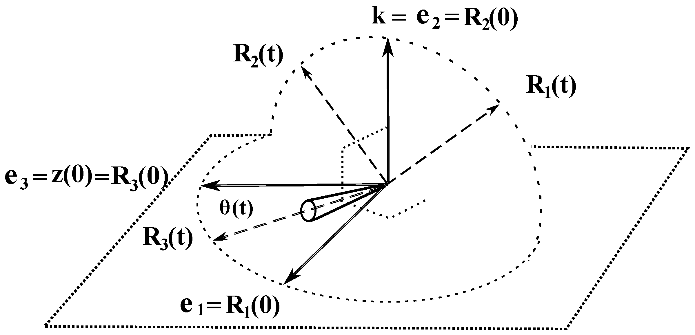
Consider a body with a fixed point subjected to the force of gravity, with the acceleration of gravity equal to $a>0$ and directed opposite to the constant unit vector $\mathbf{k}$; see Figure 1a. Then the potential energy of the body’s particle ${\mathbf{x}}_N\left(t\right)$ is $a{m}_N(\mathbf{k},{\mathbf{x}}_N\left(t\right))$. Summing up the potential energies of the body’s points, we obtain the total energy

$$\begin{array}{c}\hfill U=\sum _{N=1}^{N}a{m}_N(\mathbf{k},{\mathbf{x}}_N\left(t\right))=b(\mathbf{k},\mathbf{z}\left(t\right))=b(\mathbf{k},R\left(t\right)\mathbf{z}\left(0\right)),b\equiv aL\mu .\end{array}$$

(15)

Figure 1. (a) Initial position of a heavy body with orthogonal inertia axes ${\mathbf{R}}_1\left(0\right),{\mathbf{R}}_2\left(0\right),{\mathbf{R}}_3\left(0\right)$. (b) For the symmetric body, due to the freedom in the choice of ${\mathbf{R}}_1\left(0\right)$ and ${\mathbf{R}}_2\left(0\right)$, the vector $\mathbf{k}$ can be taken in the form $\mathbf{k}=(0,k_2,k_3)$.

Here L is the distance from the centre of mass to the fixed point, $\mu$ is the total mass of the body, and $\mathbf{z}\left(0\right)$ is the unit vector in the direction of the centre of mass at $t=0$. Accounting for the potential energy in the action (2), we obtain the variational problem for the heavy body. This implies the equations of motion

$$\begin{array}{c}\hfill m_A{\ddot{\mathbf{x}}}_A=\sum _{B=1}^3{\lambda }_{AB}{\mathbf{x}}_B+\sum _{\beta =4}^n{\lambda }_{A\beta }{\mathbf{x}}_{\beta }-{am}_A\mathbf{k},m_{\alpha }{\ddot{\mathbf{x}}}_{\alpha }=\sum _{A=1}^3{\lambda }_{A\alpha }{\mathbf{x}}_A-{am}_{\alpha }\mathbf{k}.\end{array}$$

(16)

Contrary to the free equations, we now have only two integrals of motion. Due to torque of gravity, the components of angular momentum are not conserved as follows:

$$\begin{array}{c}\hfill \dot{\mathbf{m}}=b[\mathbf{k},\mathbf{z}\left(t\right)].\end{array}$$

(17)

So, the only conserved quantities are the energy and projection of angular momentum on the direction of constant vector $\mathbf{k}$

$$\begin{array}{c}\hfill \frac{dE}{dt}=0,\mathrm{where}E=\frac{1}{2}\sum _{N=1}^n{m}_N{\dot{\mathbf{x}}}_N^2+b(\mathbf{k},\mathbf{z}\left(t\right)),\end{array}$$

(18)

$$\begin{array}{c}\hfill \frac{d}{dt}(\mathbf{k},\mathbf{m})=0,\mathrm{where}\mathbf{m}=\sum _{N=1}^n{m}_N[{\mathbf{x}}_N,{\dot{\mathbf{x}}}_N].\end{array}$$

(19)

Accounting for the potential energy in the action (9), we obtain the variational problem for the rotational degrees of freedom

$$\begin{array}{c}\hfill S=\int dt\frac{1}{2}{g}_{ij}{\dot{R}}_{ki}{\dot{R}}_{kj}-\frac{1}{2}{\lambda }_{ij}\left[R_{ki}{R}_{kj}-{\delta }_{ij}\right]-b{R}_{ij}\left(t\right)k_i{z}_j\left(0\right).\end{array}$$

(20)

This implies second-order dynamical equations

$$\begin{array}{c}\hfill {\ddot{R}}_{ik}{g}_{kj}=-R_{ik}{\lambda }_{kj}-b{k}_i{z}_j\left(0\right).\end{array}$$

(21)

Let the initial position of the inertia axes ${\mathbf{R}}_i\left(0\right)$ of the body be as shown in Figure 1a. Assuming that the laboratory axes ${\mathbf{e}}_i$ have been chosen in the direction of the inertia axes at $t=0$, the matrices $g_{ij}$ and $I_{ij}$ in all equations acquire the diagonal form.

Performing the calculations similar to those of Section V of the work in [1], we can exclude the auxiliary variables ${\lambda }_{ij}$

$$\begin{array}{c}\hfill {\lambda }_{ij}=\frac{2g_i{g}_j}{g_i+g_j}({\dot{\mathbf{R}}}_i,{\dot{\mathbf{R}}}_i)-\frac{g_i({\mathbf{R}}_i,{\mathbf{F}}_j)+g_j({\mathbf{R}}_j,{\mathbf{F}}_i)}{g_i+g_j},\mathrm{where}{\left({\mathbf{F}}_j\right)}_i\equiv b{k}_i{z}_j\left(0\right),\end{array}$$

(22)

and write second-order closed equations for $R_{ij}$. The equivalent first-order system is given then by $3+9$ equations

$$\begin{array}{c}\hfill I\dot{\mathbf{\Omega }}=[I\mathbf{\Omega },\mathbf{\Omega }]+b[R^T\mathbf{k},\mathbf{z}\left(0\right)],\end{array}$$

(23)

$$\begin{array}{c}\hfill {\dot{R}}_{ij}=-{ϵ}_{jkm}{\mathrm{\Omega }}_k{R}_{im},\mathrm{or}{\dot{\mathbf{G}}}_i=-[\mathbf{\Omega },{\mathbf{G}}_i],\end{array}$$

(24)

whereby ${\mathbf{G}}_i$ denote the rows of rotation matrix ${\left({\mathbf{G}}_i\right)}_j=R_{ij}$. From the line $\mathbf{k}={(k_1,k_2,k_3)}^T={\mathbf{e}}_i{k}_i={\mathbf{e}}_i{R}_{ij}{\left(R^T\mathbf{k}\right)}_j={\mathbf{R}}_j{\left(R^T\mathbf{k}\right)}_j$, we conclude that the functions $K_j\left(t\right)\equiv {\left(R^T\mathbf{k}\right)}_j$ in Equation (23) are components of the vector $\mathbf{k}$ in the body-fixed basis.

For the latter use we mention the identities

$$\begin{array}{c}\hfill R^T\mathbf{k}=k_i{\mathbf{G}}_i,{[R^T\mathbf{k},\mathbf{z}\left(0\right)]}_i=\left({\mathbf{R}}_i[\mathbf{k},\mathbf{z}\left(t\right)]\right).\end{array}$$

(25)

They can be used to represent the torque of gravity in various equivalent forms.

Similar to a free body, the Euler Equation (23) is equivalent to Equation (17). Indeed, for the angular momentum in the body $\mathbf{M}=R^T\mathbf{m}$, Equation (17) implies

$$\begin{array}{c}\hfill \dot{\mathbf{M}}=-[I^{-1}\mathbf{M},\mathbf{M}]+b[R^T\mathbf{k},\mathbf{z}\left(0\right)].\end{array}$$

(26)

Since $\mathbf{M}=I\mathbf{\Omega }$, these are just the Euler equations.

Hamiltonian character of Euler–Poisson equations. Equations (23) and (24) represent a Hamiltonian system [23,24,25]. This can be confirmed by constructing the Hamiltonian formulation of the Lagrangian theory (20) with the help of intermediate formalism developed in [26]. This gives the Hamiltonian

$$\begin{array}{c}\hfill H=\frac{1}{2}{I}_{ij}{\mathrm{\Omega }}_i{\mathrm{\Omega }}_j+b{R}_{ij}{k}_i{z}_j\left(0\right),\end{array}$$

(27)

where ${\mathrm{\Omega }}_j$ are Hamiltonian counterparts of angular velocity in the body. The corresponding symplectic structure on phase space with the coordinates $R_{ij},{\mathrm{\Omega }}_k$ reads as follows:

$$\begin{array}{c}\hfill \{R_{ij},R_{kn}\}=0,\{{\mathrm{\Omega }}_i,{\mathrm{\Omega }}_j\}=-\frac{I_k}{I_i{I}_j}{ϵ}_{ijk}{\mathrm{\Omega }}_k,\{{\mathrm{\Omega }}_i,R_{jk}\}=-\frac{1}{I_i}{ϵ}_{ikm}{R}_{jm}.\end{array}$$

(28)

They coincide with the brackets suggested by Chetaev [27,28] as a symplectic structure of the theory (23) and (24); see [1] for the details. By construction, the brackets are degenerate, and ${\left(R{R}^T\right)}_{ij}$ are their Casimir functions. In the Hamiltonian formalism, the Euler–Poisson equations acquire the form ${\dot{q}}^A=\{q^A,H\}$, where $q^A$ is the set of phase-space variables $R_{ij},{\mathrm{\Omega }}_k$.

Partial separation of variables in basic equations and the Euler–Poisson equations. Assuming $k_3\ne 0$, consider the change of variables

$$\begin{array}{c}\hfill (\mathbf{\Omega },{\mathbf{G}}_1,{\mathbf{G}}_2,{\mathbf{G}}_3)\to (\mathbf{\Omega },{\mathbf{G}}_1,{\mathbf{G}}_2,\mathbf{K}),\mathrm{where}\mathbf{K}=k_i{\mathbf{G}}_i=R^T\mathbf{k}.\end{array}$$

(29)

Using the identities (25) we can separate $3+3$ Euler–Poisson equations of the system (23) and (24)

$$\begin{array}{c}\hfill I\dot{\mathbf{\Omega }}=[I\mathbf{\Omega },\mathbf{\Omega }]+b[\mathbf{K},\mathbf{z}\left(0\right)],\end{array}$$

(30)

$$\begin{array}{c}\hfill \dot{\mathbf{K}}=-[\mathbf{\Omega },\mathbf{K}],\end{array}$$

(31)

from the remaining $3+3$ equations

$$\begin{array}{c}\hfill {\dot{\mathbf{G}}}_1=-[\mathbf{\Omega },{\mathbf{G}}_1],{\dot{\mathbf{G}}}_2=-[\mathbf{\Omega },{\mathbf{G}}_2].\end{array}$$

(32)

Using (7), the integrals of motion (18), (19) can be rewritten as the integrals of motion of the system (30) and (31) as follows:

$$\begin{array}{c}\hfill E=\frac{1}{2}{I}_i{\mathrm{\Omega }}_i^2+b(\mathbf{K},\mathbf{z}\left(0\right)),(\mathbf{k},\mathbf{m})=(\mathbf{K},I\mathbf{\Omega }),{\mathbf{K}}^2=1.\end{array}$$

(33)

The Equations (30) and (31) also form a Hamiltonian system with the Hamiltonian and brackets defined as follows:

$$\begin{array}{c}\hfill H=\frac{1}{2}{I}_{ij}{\mathrm{\Omega }}_i{\mathrm{\Omega }}_j+b(\mathbf{K},\mathbf{z}\left(0\right)),\end{array}$$

(34)

$$\begin{array}{c}\hfill \{K_i,K_j\}=0,\{{\mathrm{\Omega }}_i,{\mathrm{\Omega }}_j\}=-\frac{I_k}{I_i{I}_j}{ϵ}_{ijk}{\mathrm{\Omega }}_k,\{{\mathrm{\Omega }}_i,K_k\}=-\frac{1}{I_i}{ϵ}_{ikm}{K}_m.\end{array}$$

(35)

Here ${\mathbf{K}}^2$ turns out to be the Casimir function of the brackets.

We emphasize once again that for asymmetric body $I_1\ne I_2\ne I_3$ there is no more a freedom to simplify the equations using a rotation of the laboratory frame. In particular, the torque in Equation (30) generally contains all three components of the vector $\mathbf{K}$. In component form, the Equations (30) and (31) read as follows:

$$\begin{array}{c}\hfill {\dot{\mathrm{\Omega }}}_1=\frac{I_2-I_3}{I_1}{\mathrm{\Omega }}_2{\mathrm{\Omega }}_3+\frac{b}{I_1}(K_2{z}_3-K_3{z}_2),\end{array}$$

$$\begin{array}{c}\hfill {\dot{\mathrm{\Omega }}}_2=\frac{I_3-I_1}{I_2}{\mathrm{\Omega }}_1{\mathrm{\Omega }}_3+\frac{b}{I_2}(K_3{z}_1-K_1{z}_3),\end{array}$$

$$\begin{array}{c}\hfill {\dot{\mathrm{\Omega }}}_3=\frac{I_1-I_2}{I_3}{\mathrm{\Omega }}_1{\mathrm{\Omega }}_2+\frac{b}{I_3}(K_1{z}_2-K_2{z}_1),\end{array}$$

(36)

$$\begin{array}{c}\hfill {\dot{K}}_1={\mathrm{\Omega }}_3{K}_2-{\mathrm{\Omega }}_2{K}_3,{\dot{K}}_2=-{\mathrm{\Omega }}_3{K}_1+{\mathrm{\Omega }}_1{K}_3,{\dot{K}}_3={\mathrm{\Omega }}_2{K}_1-{\mathrm{\Omega }}_1{K}_2.\end{array}$$

(37)

Their formal solution can be written in terms of the exponential of the Hamiltonian vector field; see [26]. For the centre of mass vector $\mathbf{z}\left(0\right)$ in a general position, the solution to these equations in quadratures is not known. There are two special cases when the solution can be found in quadratures: Lagrange and Kovalevskaya tops. The Lagrange top will be discussed in the next section. The discussion of the Kovalevskaya top [29] in modern form can be found in [30].

4. Lagrange Top

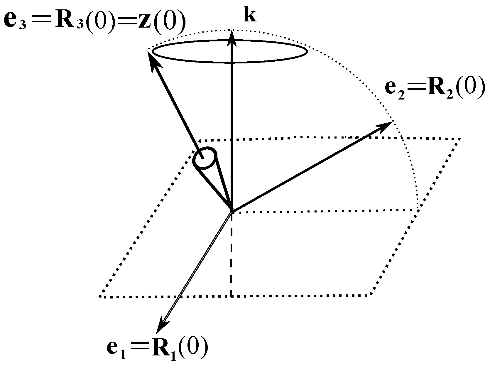
Let us take a symmetric body, that is, $I_1=I_2\ne I_3$. Then the Euler Equation (23) can be simplified as follows: without loss of generality, we can assume that the vector $\mathbf{k}$ has the following form: $\mathbf{k}=(0,k_2,k_3)$. Indeed, the eigenvectors and eigenvalues of the inertia tensor I obey the relations ${I\mathbf{R}}_i\left(0\right)=I_i{\mathbf{R}}_i\left(0\right)$. With $I_1=I_2$ we have ${I\mathbf{R}}_1\left(0\right)=I_2{\mathbf{R}}_1\left(0\right)$ and $I{\mathbf{R}}_2\left(0\right)=I_2{\mathbf{R}}_2\left(0\right)$, then any linear combination $\alpha {\mathbf{R}}_1\left(0\right)+\beta {\mathbf{R}}_2\left(0\right)$ also represents an eigenvector with eigenvalue $I_2$. This means that we are free to choose any two orthogonal axes on the plane ${\mathbf{R}}_1\left(0\right),{\mathbf{R}}_2\left(0\right)$ as the inertia axes. Hence, in the case $I_1=I_2$ we can rotate the laboratory axes in the plane $(x^1,x^2)$ without breaking the diagonal form of the inertia tensor. Using this freedom, we can assume that $k_1=0$ for our problem; see Figure 1b.

Moving to the case of the Lagrange top, we further assume that the fixed point of the symmetric body was chosen such that the centre of mass lies on the third axis of inertia. Then at the initial instant of time we have $\mathbf{z}\left(0\right)={(0,0,1)}^T$. Substituting $\mathbf{k}={(0,k_2,k_3)}^T$ and $\mathbf{z}\left(0\right)={(0,0,1)}^T$ into the Euler Equation (23), we obtain

$$\begin{array}{c}\hfill {\dot{\mathrm{\Omega }}}_1=\varphi {\mathrm{\Omega }}_2+\frac{b}{I_2}(k_2{R}_{22}+k_3{R}_{32}),{\dot{\mathrm{\Omega }}}_2=-\varphi {\mathrm{\Omega }}_1-\frac{b}{I_2}(k_2{R}_{21}+k_3{R}_{31}),{\dot{\mathrm{\Omega }}}_3=0,\end{array}$$

(38)

where $\varphi =\frac{I_2-I_3}{I_2}{\mathrm{\Omega }}_3=\mathrm{const}$. Together with (24), they represent equations of motion of the Lagrange top. The last equation from (38) implies that besides the integrals of motion (18) and (19), there is one more: ${\mathrm{\Omega }}_3=\mathrm{const}$. This can also be seen from Equation (26). Indeed, the third component of this equation reads as follows:

$$\begin{array}{c}\hfill {\dot{M}}_3=\left(\frac{1}{I_2}-\frac{1}{I_1}\right)M_1{M}_2-b(\mathbf{k},[{\mathbf{R}}_3\left(t\right),\mathbf{z}\left(t\right)]).\end{array}$$

(39)

For the Lagrange top we have $I_1=I_2$ and $\mathbf{z}\left(t\right)={\mathbf{R}}_3\left(t\right)$, so ${\dot{M}}_3=I_3{\dot{\mathrm{\Omega }}}_3=0$.

Variational problem for the Lagrange top in terms of Euler angles. Let us write the Lagrangian (20) as follows:

$$\begin{array}{c}\hfill L=\frac{1}{2}{I}_i{\left({\mathrm{\Omega }}_i\right)}^2-\frac{1}{2}{\lambda }_{ij}\left[R_{ki}{R}_{kj}-{\delta }_{ij}\right]-b{R}_{ij}\left(t\right)k_i{z}_j\left(0\right),\end{array}$$

(40)

where ${\mathrm{\Omega }}_i\equiv -\frac{1}{2}{ϵ}_{ijk}{\left(R^T\dot{R}\right)}_{jk}$. Let us substitute the expression for $R_{ij}$ in terms of Euler angles

$$\begin{array}{c}\hfill R=\left(\begin{array}{ccc}cos\psi cos\phi -sin\psi cos\theta sin\phi & -sin\psi cos\phi -cos\psi cos\theta sin\phi & sin\theta sin\phi \\ cos\psi sin\phi +sin\psi cos\theta cos\phi & -sin\psi sin\phi +cos\psi cos\theta cos\phi & -sin\theta cos\phi \\ sin\psi sin\theta & cos\psi sin\theta & cos\theta \end{array}\right)\end{array}$$

(41)

into Equation (40). According to classical mechanics (see Section 17 in [10] or Section 1.6 in [25]), this gives an equivalent variational problem. Since the rotation matrix in terms of Euler angles automatically obeys the constraint $R^{T}R=\mathbf{1}$, the second term of the action (40) vanishes, and we obtain

$$\begin{array}{c}\hfill L=\frac{1}{2}{I}_2[{\dot{\theta }}^2+{\dot{\phi }}^2{sin}^2\theta ]+\frac{1}{2}{I}_3{[\dot{\psi }+\dot{\phi }cos\theta ]}^2-b{R}_{ij}(\theta ,\phi ,\psi )k_i{z}_j\left(0\right).\end{array}$$

(42)

As we saw above, the Lagrange top corresponds to the choice $\mathbf{z}\left(0\right)=(0,0,1)$ and $k=(0,k_2,k_3)$. With these $\mathbf{z}\left(0\right)$ and $\mathbf{k}$, the potential energy acquires the form $b(k_2{R}_{23}+k_3{R}_{33})$, and we obtain the variational problem for the Lagrange top in terms of Euler angles

$$\begin{array}{c}\hfill L=\frac{1}{2}{I}_2[{\dot{\theta }}^2+{\dot{\phi }}^2{sin}^2\theta ]+\frac{1}{2}{I}_3{[\dot{\psi }+\dot{\phi }cos\theta ]}^2-b[k_{3}cos\theta -k_{2}sin\theta cos\phi ].\end{array}$$

(43)

This gives the following equations of motion:

$$\begin{array}{c}\hfill I_3[\dot{\psi }+\dot{\phi }cos\theta ]=m_{\psi }=\mathrm{const},\end{array}$$

(44)

$$\begin{array}{c}\hfill \frac{d}{dt}[I_2\dot{\phi }{sin}^2\theta +m_{\psi }cos\theta ]+b{k}_{2}sin\theta sin\phi =0,\end{array}$$

(45)

$$\begin{array}{c}\hfill -I_2\ddot{\theta }+I_2{\dot{\phi }}^{2}sin\theta cos\theta -m_{\psi }sin\theta \dot{\phi }+b[k_{3}sin\theta +k_{2}cos\theta cos\phi ]=0.\end{array}$$

(46)

In many textbooks [3,4,5,6,7,8], authors considered other equations following from a different Lagrangian [9,10]; the latter does not contain the term proportional to $k_2$:

$$\begin{array}{c}\hfill L_A=\frac{1}{2}{I}_2[{\dot{\theta }}^2+{\dot{\phi }}^2{sin}^2\theta ]+\frac{1}{2}{I}_3{[\dot{\psi }+\dot{\phi }cos\theta ]}^2-bcos\theta .\end{array}$$

(47)

This term is discarded on the basis of the following reasoning: to simplify the analysis, choose the laboratory axis ${\mathbf{e}}_3$ in the direction of gravity vector $\mathbf{k}$. However, this reasoning does not take into account the presence in the equations of moments of inertia, which have the tensor law of transformation under rotations. Indeed, going back to Equations (23) and (24), select ${\mathbf{e}}_3$ in Figure 1b in the direction of $\mathbf{k}$, and calculate the components of the inertia tensor. Since the axis of inertia ${\mathbf{R}}_3\left(0\right)$ does not coincide with ${\mathbf{e}}_3$, we obtain a symmetric matrix with non-zero off-diagonal elements (12) instead of (14). This symmetric matrix should now be used to construct the kinetic part of Lagrangian and hence, it appears in the equations of motion. That is, the attempt to simplify the potential energy will lead to a Lagrangian with a complicated expression for the kinetic energy, rather than to (47).

Does a rotating body have motions that could be described using the equations following from an incomplete Lagrangian (47)? The answer is yes: these are solutions with special initial data, for which the ${\mathbf{R}}_3\left(t\right)$ axis coincides with $\mathbf{k}$ at some (finite) instant in time. These are the solutions of an awakened top and its limiting case of a sleeping top; see below. In the general case, to look for the solutions with ${\mathbf{R}}_3\left(t\right)$ that do not pass through $\mathbf{k}$, one should use the equations following from (43).

Probably for the first time in the monographic literature, the equations following from incomplete Lagrangian (47) were discussed in detail by MacMillan in [4]. In the absence of an analytical solution in elementary functions, MacMillan performed an analysis of integrals of motion and effective potential, reducing the problem to the study of a polynomial of degree 3. The results of this qualitative analysis are summarized in Figures 60–62 of his book, and then reproduced in many other textbooks. In this respect we point out that a similar analysis of the improved Lagrangian (43) leads to the study of a polynomial of degree 6; see [20].

5. Sleeping Lagrange Top

Consider the Lagrange top that at $t=0$ has its centre of mass vector in the direction of gravity vector $\mathbf{k}$, and was launched with initial angular velocity ${\mathrm{\Omega }}_0$ = const around the axis $\mathbf{k}$. In accordance with this, we use $\mathbf{z}\left(0\right)=\mathbf{k}={(0,0,1)}^T$ and $\mathbf{\Omega }\left(0\right)=(0,0,{\mathrm{\Omega }}_0)$ in Equations (23) and (24). The equations for $\mathrm{\Omega }\left(t\right)$ and ${\mathbf{R}}_3\left(t\right)$ read as follows:

$$\begin{array}{c}\hfill {\dot{\mathrm{\Omega }}}_1=\varphi {\mathrm{\Omega }}_2+\frac{b}{I_2}{R}_{32},{\dot{\mathrm{\Omega }}}_2=-\varphi {\mathrm{\Omega }}_1-\frac{b}{I_2}{R}_{31},{\dot{\mathrm{\Omega }}}_3=0;\end{array}$$

$$\begin{array}{c}\hfill {\dot{R}}_{31}=R_{32}{\mathrm{\Omega }}_3-R_{33}{\mathrm{\Omega }}_2,{\dot{R}}_{32}=R_{33}{\mathrm{\Omega }}_1-R_{31}{\mathrm{\Omega }}_3,{\dot{R}}_{33}=R_{31}{\mathrm{\Omega }}_2-R_{32}{\mathrm{\Omega }}_1,\end{array}$$

(48)

where $\varphi =\frac{I_2-I_3}{I_2}{\mathrm{\Omega }}_3$. They are satisfied by the functions $\mathbf{\Omega }\left(t\right)=(0,0,{\mathrm{\Omega }}_0)$, $R_{31}\left(t\right)=R_{32}\left(t\right)=0$ and $R_{33}\left(t\right)=1$. Then the remaining equations from (23) and (24) are

$$\begin{array}{c}\hfill {\dot{R}}_{11}=R_{12}{\mathrm{\Omega }}_0,{\dot{R}}_{12}=-R_{11}{\mathrm{\Omega }}_0,{\dot{R}}_{13}=0;\end{array}$$

$$\begin{array}{c}\hfill {\dot{R}}_{21}=R_{22}{\mathrm{\Omega }}_0,{\dot{R}}_{22}=-R_{21}{\mathrm{\Omega }}_0,{\dot{R}}_{23}=0.\end{array}$$

(49)

Their general solution is

$$\begin{array}{c}\hfill R_{11}=Acos{\mathrm{\Omega }}_{0}t+Bsin{\mathrm{\Omega }}_{0}t,R_{12}=-Asin{\mathrm{\Omega }}_{0}t+Bcos{\mathrm{\Omega }}_{0}t,R_{13}=F;\end{array}$$

$$\begin{array}{c}\hfill R_{21}=Ccos{\mathrm{\Omega }}_{0}t+Dsin{\mathrm{\Omega }}_{0}t,R_{22}=-Csin{\mathrm{\Omega }}_{0}t+Dcos{\mathrm{\Omega }}_{0}t,R_{23}=G.\end{array}$$

(50)

Taking into account the initial data $R_{ij}\left(0\right)={\delta }_{ij}$, we obtain $A=D=1$, $B=C=F=G=0$, and the solution is the stationary rotation around the vector of gravity $\mathbf{k}$:

$$\begin{array}{c}\hfill R_{ij}\left(t\right)=\left(\begin{array}{ccc}cos{\mathrm{\Omega }}_{0}t& -sin{\mathrm{\Omega }}_{0}t& 0\\ sin{\mathrm{\Omega }}_{0}t& cos{\mathrm{\Omega }}_{0}t& 0\\ 0& 0& 1\end{array}\right).\end{array}$$

(51)

6. Awakened Lagrange Top

Consider the Lagrange top that at $t=0$ has its centre of mass vector in the direction of gravity vector $\mathbf{k}$, so $\mathbf{z}\left(0\right)=\mathbf{k}={(0,0,1)}^T$. Substituting these values into Equation (40) we obtain the following variational problem in terms of Euler angles

$$\begin{array}{c}\hfill L=\frac{1}{2}{I}_2[{\dot{\theta }}^2+{\dot{\phi }}^2{sin}^2\theta ]+\frac{1}{2}{I}_3{[\dot{\psi }+\dot{\phi }cos\theta ]}^2-bcos\theta .\end{array}$$

(52)

The initial data should be formulated now for the Euler angles. Let the top be launched from a vertical position with some linear velocity ${\dot{\mathbf{R}}}_3\left(0\right)$. This vector is parallel to the plane of the laboratory vectors ${\mathbf{e}}_1$ and ${\mathbf{e}}_2$. Using the freedom to rotate the laboratory system in the plane of these vectors without spoiling the diagonal form of the inertia tensor, we can assume that ${\dot{\mathbf{R}}}_3\left(0\right)$ is antiparallel to ${\mathbf{e}}_2$. With these agreements, consider the top with the initial position $\theta \left(0\right)=\phi \left(0\right)=\psi \left(0\right)=0$, and with the initial nutation $\dot{\theta }\left(0\right)={\dot{\theta }}_0$ and rotation $\dot{\psi }\left(0\right)={\dot{\psi }}_0$, where ${\dot{\theta }}_0<<{\dot{\psi }}_0$. We do not fix the speed of precession $\dot{\phi }\left(0\right)$ of the azimuth plane because it is determined by ${\dot{\psi }}_0$; see Equation (57) below. The Lagrangian (52) does not depend on $\psi$ and $\phi$, so the equations of motion $\delta S/\delta \psi =0$ and $\delta S/\delta \phi =0$ give the integrals of motion $m_{\psi }$ and $m_{\phi }$:

$$\begin{array}{c}\hfill I_3[\dot{\psi }+\dot{\phi }cos\theta ]=m_{\psi }=\mathrm{const},\mathrm{then}{m}_{\psi }=I_3[{\dot{\psi }}_0+{\dot{\phi }}_0],\end{array}$$

(53)

$$\begin{array}{c}\hfill I_2\dot{\phi }{sin}^2\theta +m_{\psi }cos\theta =m_{\phi }=\mathrm{const}.\end{array}$$

(54)

Substituting the initial data $\theta \left(0\right)=0$ into the last equation, we conclude that the integrals of motion are not independent:

$$\begin{array}{c}\hfill m_{\phi }=m_{\psi }.\end{array}$$

(55)

Taking this into account, Equation (54) reads

$$\begin{array}{c}\hfill \dot{\phi }=\frac{m_{\psi }}{I_2(1+cos\theta )}.\end{array}$$

(56)

This implies that $\dot{\phi }$ is a non-negative function, so the azimuth plane cannot change its direction of rotation during the motion of the top. In addition, from the above expressions we obtain the initial speed ${\dot{\phi }}_0$ and then the integral of motion $m_{\psi }$ through the initial rotation ${\dot{\psi }}_0$:

$$\begin{array}{c}\hfill {\dot{\phi }}_0=\frac{I_3}{2I_2-I_3}{\dot{\psi }}_0,m_{\psi }=\frac{2I_2{I}_3}{2I_2-I_3}{\dot{\psi }}_0.\end{array}$$

(57)

Variation of the Lagrangian (52) with respect to $\theta$ gives the second-order equation

$$\begin{array}{c}\hfill -I_2\ddot{\theta }+I_2{\dot{\phi }}^{2}sin\theta cos\theta -I_3[\dot{\psi }+\dot{\phi }cos\theta ]\dot{\phi }sin\theta +bsin\theta =0.\end{array}$$

(58)

Using Equations (53) and (57), we exclude the variables $\phi$ and $\psi$, obtaining closed equation for $\theta$:

$$\begin{array}{c}\hfill -I_2\ddot{\theta }-\frac{m_{\psi }^2}{I_2}\frac{sin\theta }{{(1+cos\theta )}^2}+bsin\theta =0.\end{array}$$

(59)

This equation follows from the effective Lagrangian

$$\begin{array}{c}\hfill L_{eff}=\frac{I_2}{2}{\dot{\theta }}^2-\frac{m_{\psi }^2}{I_2(1+cos\theta )}-bcos\theta .\end{array}$$

(60)

The energy of this effective one-dimensional problem is an integral of motion

$$\begin{array}{c}\hfill \frac{I_2}{2}{\dot{\theta }}^2+\frac{m_{\psi }^2}{I_2(1+cos\theta )}+bcos\theta =E=\mathrm{const},\mathrm{then}E=\frac{1}{2}[I_2{\dot{\theta }}_0^2+\frac{m_{\psi }^2}{I_2}]+b.\end{array}$$

(61)

This allows us to write the first-order equation for $\theta$:

$$\begin{array}{c}\hfill \dot{\theta }=\sqrt{\frac{2}{I_2}}\sqrt{\frac{(E-bcos\theta )(1+cos\theta )-\gamma }{1+cos\theta }},\mathrm{where}\gamma \equiv \frac{m_{\psi }^2}{I_2},\end{array}$$

(62)

that can be immediately integrated as follows:

$$\begin{array}{c}\hfill \int \frac{dx}{\sqrt{x\left[\right(E-b+bx\left)\right(2-x)-\gamma ]}}=\sqrt{\frac{2}{I_2}}\int dt,\mathrm{where}x\equiv 1-cos\theta .\end{array}$$

(63)

So, the problem was reduced to the elliptic integral, which appeared in the last expression.

In the absence of an analytic solution in elementary functions, we can use the effective one-dimensional problem (60) for qualitative analysis of the motion. Consider a top of mass $\mu =0.1$ kg, in the form of a cone of height $h=0.12$ m and radius $r=0.06$ m. As the fixed point, we take the vertex of the cone. Then the distance to the centre of mass and the inertia moments are as follows [9]:

$$\begin{array}{c}\hfill L=\frac{3h}{4}=0.09m,I_1=I_2=\frac{3}{5}\mu (\frac{r^2}{4}+h^2)=918\times {10}^{-6},I_3=\frac{3}{10}\mu r^2=108\times {10}^{-6}.\end{array}$$

(64)

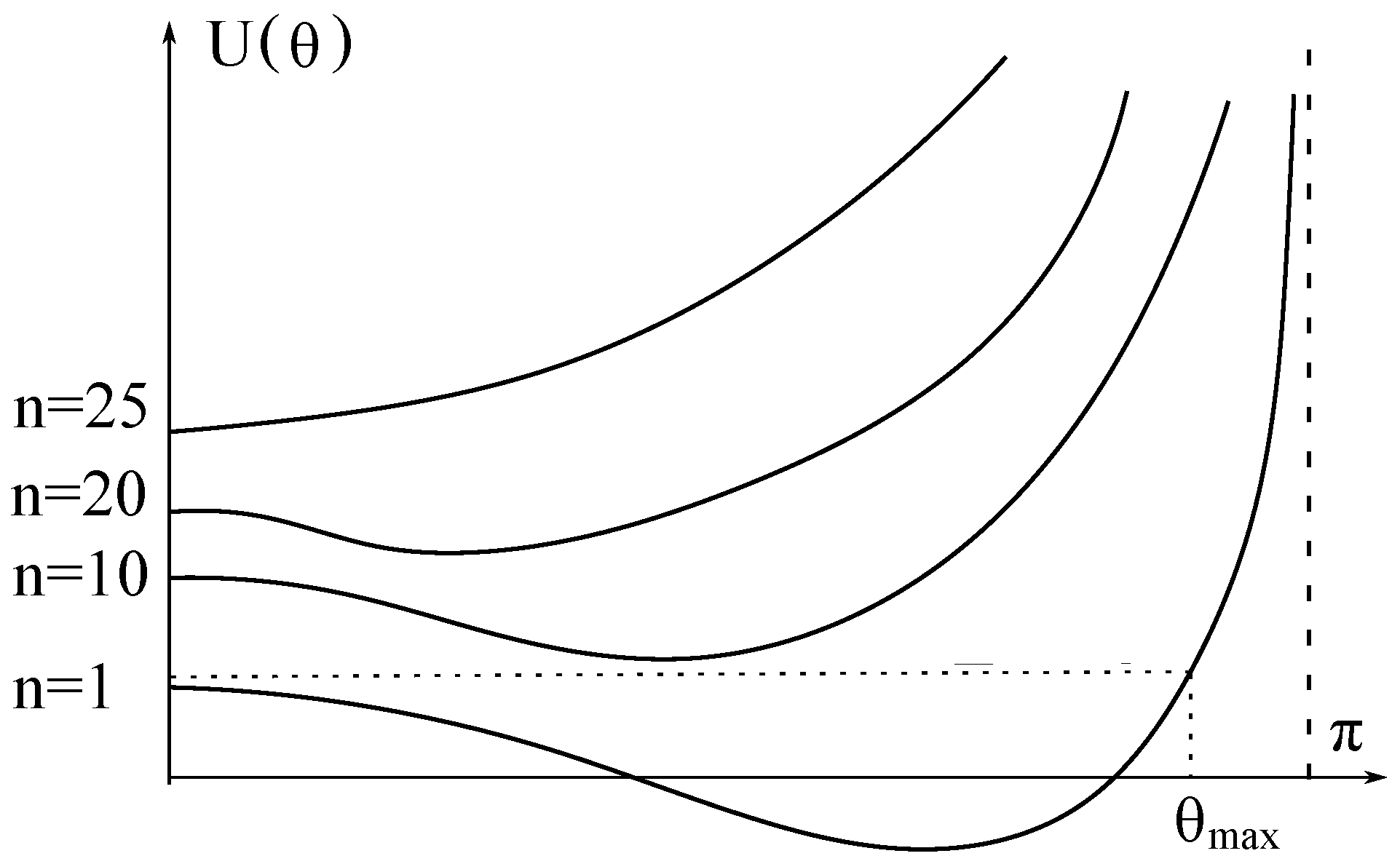
As the initial velocities of rotation and nutation we take ${\dot{\psi }}_0=2\pi n$ rad/s and ${\dot{\theta }}_0=0.2$ rad/s$\sim {11}^{\circ }$/s, where n is the number of revolutions per second. The potential energy of the effective problem (60) reads

$$\begin{array}{c}\hfill U_{eff}\left(\theta \right)=\frac{\gamma }{1+cos\theta }+bcos\theta ,\mathrm{where}\gamma \equiv \frac{m_{\psi }^2}{I_2}=0.565694455\times {10}^{-3},b=a\mu L=0.0882.\end{array}$$

(65)

Typical graphs of the function $U_{eff}\left(\theta \right)$ are drawn in Figure 2.

Figure 2. Effective potential energy of awakened Lagrange top with initial nutation rate ${\dot{\theta }}_0={11}^{\circ }$/s.

The potential energy of a slow top has a minimum at the point $cos\theta =-1+\sqrt{\gamma /b}$, which shifts to the left with increasing rotational speed ${\dot{\psi }}_0$, so that for velocities greater than 24 revolutions per second, the point of minimum becomes $\theta =0$. The graphs show that the awakened top first deviates from the vertical position, and then returns.

The maximum deviation ${\theta }_{max}$ of the axis ${\mathbf{R}}_3\left(t\right)$ from the vertical can be found in analytical form from Equation (61), in which we should put $\dot{\theta }\left(t\right)=0$. Then

$$\begin{array}{c}\hfill cos{\theta }_{max}=\frac{\gamma +\sigma }{4b}-\sqrt{{(1+\frac{\gamma +\sigma }{4b})}^2-\frac{\gamma }{b}},\mathrm{where}\delta =I_2{\dot{\theta }}_0^2=0.3672\times {10}^{-4}.\end{array}$$

(66)

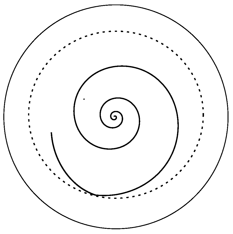
Furthermore, with the use of Equations (56) and (57) we can estimate the character of rotation of the azimuth plane by calculating the precession speed ${\dot{\phi }}_0$ and $\dot{\phi }\left({\theta }_{max}\right)$. The results of these calculations are presented in Table 1. The initial precession speed ${\dot{\phi }}_0$ of the azimuth plane grows with ${\dot{\psi }}_0$, while the precession speed $\dot{\phi }\left({\theta }_{max}\right)$ at the point of maximum deviation first decreases but then begins to increase, starting from 25 revolutions per second. The precession rate of a fast top changes slowly with time. The typical trajectory of the third axis ${\mathbf{R}}_3\left(t\right)$ is drawn in Figure 3. This should be compared with Figures 60–62 of MacMillan’s book [4].

Table 1. Maximum deviation and precession rates of awakened Lagrange top with initial nutation rate ${\dot{\theta }}_0={11}^{\circ }$/s.

${\dot{\mathit{\psi }}}_0=\mathit{n}$ rev./s	${{\mathit{\theta }}_{\mathit{max}}}^{\circ }$	${\dot{\mathit{\phi }}}_0$ rev./s	$\dot{\mathit{\phi }}\left({\mathit{\theta }}_{\mathit{max}}\right)$ rev./s
1	175	0.0625	39
10	131	0.625	3.9
13	117	0.8	3.0
16	103	1	2.44
20	74	1.25	1.95
23	46	1.43	1.7
25	11	1.56	1.58
26	4	1.62	1.62

Figure 3. Trajectory of the axis ${\mathbf{R}}_3\left(t\right)$ (from vertical to the maximum deviation position) of awakened Lagrange top with initial nutation rate ${\dot{\theta }}_0={11}^{\circ }$/s.

7. Horizontal Precession around Gravity Vector

Consider the Lagrange top that at $t=0$ has its third axis ${\mathbf{R}}_3\left(0\right)$ orthogonal to the gravity vector $\mathbf{k}$; see Figure 4.

Figure 4. Horizontal precession of the Lagrange top around gravity vector.

Using the freedom of rotation of the laboratory axes in the plane ${\mathbf{e}}_1,{\mathbf{e}}_2$, we can assume that $\mathbf{k}={\mathbf{e}}_2={(0,1,0)}^T$. Substituting these values together with $\mathbf{z}\left(0\right)={(0,0,1)}^T$ into the Lagrangian (42), we obtain

$$\begin{array}{c}\hfill L=\frac{1}{2}{I}_2[{\dot{\theta }}^2+{\dot{\phi }}^2{sin}^2\theta ]+\frac{1}{2}{I}_3{[\dot{\psi }+\dot{\phi }cos\theta ]}^2+bsin\theta cos\phi .\end{array}$$

(67)

This implies the equations

$$\begin{array}{c}\hfill I_3[\dot{\psi }+\dot{\phi }cos\theta ]=m_{\psi }=\mathrm{const},\end{array}$$

$$\begin{array}{c}\hfill \frac{d}{dt}[I_2\dot{\phi }{sin}^2\theta +m_{\psi }cos\theta ]+bsin\theta sin\phi =0,\end{array}$$

$$\begin{array}{c}\hfill -I_2\ddot{\theta }+I_2{\dot{\phi }}^{2}sin\theta cos\theta -m_{\psi }sin\theta \dot{\phi }+bcos\theta cos\phi =0.\end{array}$$

(68)

We assume that our top has some initial rotation and precession rates $\dot{\psi }\left(0\right)={\dot{\psi }}_0$ and $\dot{\theta }\left(0\right)={\dot{\theta }}_0$. Then the initial position of the top is $\theta \left(0\right)=0,\phi \left(0\right)=\frac{\pi }{2},\psi \left(0\right)=\frac{3\pi }{2}$. Let us look for a solution of the form $\theta \left(t\right),\phi \left(t\right)=\frac{\pi }{2},\psi \left(t\right)$, then the equations of motion read

$$\begin{array}{c}\hfill \dot{\psi }={\dot{\psi }}_0,\dot{\theta }=\frac{b}{I_3{\dot{\psi }}_0},\ddot{\theta }=0,\end{array}$$

(69)

and we obtain the solution $\theta \left(t\right)=\frac{b}{I_3{\dot{\psi }}_0}t,\phi \left(t\right)=\frac{\pi }{2},\psi \left(t\right)={\dot{\psi }}_{0}t+\frac{3\pi }{2}$. Substituting these functions into Equation (41), we obtain the rotation matrix which turns out to be the composition of two rotations: counterclockwise around the ${\mathbf{e}}_2$ axis and clockwise around the ${\mathbf{e}}_3$ axes

$$R\left(t\right)=\left(\begin{array}{ccc}cos{\dot{\psi }}_{0}tcos{\dot{\theta }}_{0}t& -sin{\dot{\psi }}_{0}tcos{\dot{\theta }}_{0}t& sin{\dot{\theta }}_{0}t\\ sin{\dot{\psi }}_{0}t& cos{\dot{\psi }}_{0}t& 0\\ -cos{\dot{\psi }}_{0}tsin{\dot{\theta }}_{0}t& sin{\dot{\psi }}_{0}tsin{\dot{\theta }}_{0}t& cos\alpha t\end{array}\right)=\left(\begin{array}{ccc}cos{\dot{\theta }}_{0}t& 0& sin{\dot{\theta }}_{0}t\\ 0& 1& 0\\ -sin{\dot{\theta }}_{0}t& 0& cos{\dot{\theta }}_{0}t\end{array}\right)\times \left(\begin{array}{ccc}cos{\dot{\psi }}_{0}t& -sin{\dot{\psi }}_{0}t& 0\\ sin{\dot{\psi }}_{0}t& cos{\dot{\psi }}_{0}t& 0\\ 0& 0& 1\end{array}\right),$$

(70)

where

$$\begin{array}{c}\hfill {\dot{\theta }}_0=\frac{b}{I_3{\dot{\psi }}_0}.\end{array}$$

(71)

Thus, the Lagrange top launched with the rotation rate ${\dot{\psi }}_0$ and precession rate ${\dot{\theta }}_0=\frac{b}{I_3{\dot{\psi }}_0}$ will precess around $\mathbf{k}$ in the horizontal plane. A slow spinning top must precess at high speed to stay on this plane. A fast spinning top precesses slowly. The relationship between frequencies of rotation and precession does not depend on the geometry of the top.

8. Inclined Lagrange Top: Precession around Gravity Vector without Nutation

Without loss of generality, we can choose the initial position of the inclined Lagrange top (and hence the laboratory system) as shown in Figure 5.

Figure 5. Precession without nutation of inclined Lagrange top.

According to (38) and (24), the equations of motion are

$$\begin{array}{c}\hfill {\dot{\mathrm{\Omega }}}_1=\varphi {\mathrm{\Omega }}_2+\frac{b}{I_2}(k_2{R}_{22}+k_3{R}_{32}),{\dot{\mathrm{\Omega }}}_2=-\varphi {\mathrm{\Omega }}_1-\frac{b}{I_2}(k_2{R}_{21}+k_3{R}_{31}),{\mathrm{\Omega }}_3=\mathrm{const};\end{array}$$

(72)

$$\begin{array}{c}\hfill {\dot{R}}_{ij}=-{ϵ}_{jkm}{\mathrm{\Omega }}_k{R}_{im},\end{array}$$

(73)

where $\varphi =\frac{I_2-I_3}{I_2}{\mathrm{\Omega }}_3=\mathrm{const}$. We look for the solution that represents precession around $\mathbf{k}$ without nutation; that is, $({\mathbf{R}}_3\left(t\right),\mathbf{k})=\mathrm{const}$ for any t. It can be expected that this motion be described by a rotation matrix consisting of the product of rotations around the axes $\mathbf{k}$ and ${\mathbf{e}}_3$: $R(t,\alpha ,\gamma )=R_{\mathbf{k}}(t,\gamma )\times R_{{\mathbf{e}}_3}(t,\alpha )$. Therefore, we will look for a solution in the following form (see [1] for the details):

$$\begin{array}{c}\hfill R_{ij}=\left(\begin{array}{ccc}cos\gamma tcos\alpha t-k_{3}sin\gamma tsin\alpha t& -cos\gamma tsin\alpha t-k_{3}sin\gamma tcos\alpha t& k_{2}sin\gamma t\\ & & \\ k_{3}sin\gamma tcos\alpha t+(k_2^2+k_3^{2}cos\gamma t)sin\alpha t& -k_{3}sin\gamma tsin\alpha t+(k_2^2+k_3^{2}cos\gamma t)cos\alpha t& k_2{k}_3(1-cos\gamma t)\\ & & \\ -k_{2}sin\gamma tcos\alpha t+k_2{k}_3(1-cos\gamma t)sin\alpha t& k_{2}sin\gamma tsin\alpha t+k_2{k}_3(1-cos\gamma t)cos\alpha t& k_3^2+k_2^{2}cos\gamma t\end{array}\right)\end{array}$$

(74)

with some frequencies of rotation $\alpha$ and precession $\gamma$. For the positive values of the frequencies, $R_{{\mathbf{e}}_3}(t,\alpha )$ is in a clockwise rotation while $R_{\mathbf{k}}(t,\gamma )$ is in a counterclockwise one. Substituting this matrix into Equation (72), we obtain

$$\begin{array}{c}\hfill {\dot{\mathrm{\Omega }}}_1=\varphi {\mathrm{\Omega }}_2+\frac{b{k}_2}{I_2}cos\alpha t,{\dot{\mathrm{\Omega }}}_2=-\varphi {\mathrm{\Omega }}_1-\frac{b{k}_2}{I_2}sin\alpha t.\end{array}$$

(75)

The general solution to this system with two integration constants c and ${\varphi }_0$ is ${\mathrm{\Omega }}_1=csin(\alpha t+{\varphi }_0)$, ${\mathrm{\Omega }}_2=ccos(\alpha t+{\varphi }_0)$, where

$$\begin{array}{c}\hfill \alpha =\varphi +\frac{b{k}_2}{I_{2}c}=\frac{I_2-I_3}{I_2}{\mathrm{\Omega }}_3+\frac{b{k}_2}{I_{2}c}.\end{array}$$

(76)

The initial conditions $R_{ij}\left(0\right)={\delta }_{ij}$ imply ${\varphi }_0=0$, so finally

$$\begin{array}{c}\hfill {\mathrm{\Omega }}_1=csin\alpha t,{\mathrm{\Omega }}_2=ccos\alpha t.\end{array}$$

(77)

The functions (77) and (74) with $\alpha$ given in (76) satisfy the Euler Equation (72) for arbitrary values of the constants ${\mathrm{\Omega }}_3$, c, and $\gamma$. Let us try to choose them so that our functions also satisfy the Poisson Equation (73). At $t=0$ the Equation (73) turns into ${\mathrm{\Omega }}_k\left(0\right)=-\frac{1}{2}{ϵ}_{kij}{\dot{R}}_{ij}\left(0\right)$. Substituting our functions (77) and (74) into these equalities we obtain the numbers c and ${\mathrm{\Omega }}_3$ through $\gamma$ as follows:

$$\begin{array}{c}\hfill c=k_2\gamma ,{\mathrm{\Omega }}_3=\frac{b}{I_3\gamma }+\frac{I_2{k}_3}{I_3}\gamma .\end{array}$$

(78)

Together with Equation (76), these expressions give the following relationship between the two frequencies of our problem:

$$\begin{array}{c}\hfill \alpha =\frac{A}{\gamma }+C{k}_3\gamma ,\mathrm{where}A\equiv \frac{b}{I_3}=\frac{a\mu L}{I_3}>0,C\equiv \frac{I_2-I_3}{I_3}.\end{array}$$

(79)

It is verified by direct calculations that the functions (77) and (74) with these values of c, ${\mathrm{\Omega }}_3$, and $\alpha$ satisfy the Poisson Equation (73) for any value of the precession frequency $\gamma$. Hence, the rotation matrix (74) with the rotation and precession frequencies related according to Equation (79) describes the precession without nutation of an inclined Lagrange top. Note that for the horizontal top, $k_2=1$ and $k_3=0$, the solution obtained turns into (70).

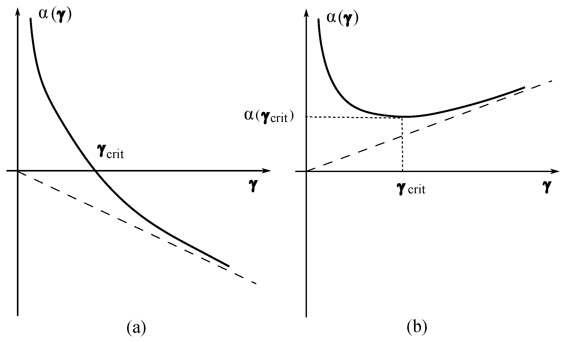
The function $\alpha \left(\gamma \right)$ depends on the top’s configuration C and inclination $k_3$. To discuss this function, consider a conical top of height h, radius r, and the precession frequency $\gamma >0$. We obtain (see Equation (64)) $I_2-I_3=\frac{3\mu }{20}[4h^2-r^2]$. So, $C>0$ when $h>r/2$ (high top), $C=0$ when $h=r/2$ (totally symmetric top, $I_1=I_2=I_3$), and $C<0$ when $h<r/2$ (low top).

Then the following cases arise.

A. The low top located above the horizon, that is

$$\begin{array}{c}\hfill 2h<r,\mathrm{then}C<0;k_3>0.\end{array}$$

(80)

The graph of the function $\alpha \left(\gamma \right)$ is drawn in Figure 6a and implies the following behaviour of the top.

Figure 6. The relationship between two frequencies. (a) Low top located above the horizon, (b) High top located above the horizon.

A1. 

Slow precession without nutation, $\gamma <{\gamma }_{crit}=\sqrt{-b/(I_2-I_3)k_3}$, implies a clockwise rotation of the top around ${\mathbf{R}}_3\left(t\right)$.

A2. 

When $\gamma ={\gamma }_{crit}$, the centripetal acceleration balances the force of gravity, and the top precesses without rotation around ${\mathbf{R}}_3\left(t\right)$.

A3. 

Rapid precession, $\gamma >{\gamma }_{crit}$, implies counterclockwise rotation around ${\mathbf{R}}_3\left(t\right)$. In the limit $\gamma \to \infty$ the rotation frequency $\left|\alpha \right|$ grows linearly with $\gamma$.

B. The high top located below the horizon

$$\begin{array}{c}\hfill 2h>r,\mathrm{then}C>0;k_3<0,\end{array}$$

(81)

has similar behaviour.

C. The high top located above the horizon

$$\begin{array}{c}\hfill 2h>r,\mathrm{then}C>0;k_3>0.\end{array}$$

(82)

The graph of the function $\alpha \left(\gamma \right)$ is drawn in Figure 6b and implies the following behaviour of the top.

C1. 

The top rotating around ${\mathbf{R}}_3\left(t\right)$ with the frequency less than $\alpha \left({\gamma }_{crit}\right)=2\sqrt{(I_2-I_3)b{k}_3}/I_3$ cannot precess without a nutation.

C2. 

There is only one rotation frequency $\alpha \left({\gamma }_{crit}\right)$ at which the top’s precession frequency is ${\gamma }_{crit}=\sqrt{b/(I_2-I_3)k_3}$.

C3. 

For each $\alpha >\alpha \left({\gamma }_{crit}\right)$, there are two possible precession frequencies for the movement without nutation

$$\begin{array}{c}\hfill \gamma =\frac{\alpha \pm \sqrt{{\alpha }^2-4AC{k}_3}}{2C{k}_3}.\end{array}$$

(83)

D. The low top located below the horizon

$$\begin{array}{c}\hfill 2h<r,\mathrm{then}C<0;k_3<0,\end{array}$$

(84)

has similar behaviour.

E. The totally symmetrical conical top

$$\begin{array}{c}\hfill 2h=r,\mathrm{then}{I}_1=I_2=I_3,C=0,\alpha =\frac{b}{I_3\gamma },\end{array}$$

(85)

has behaviour similar to the horizontal top. The relationship between two frequencies does not depend on the top’s inclination $k_3$.

9. Conclusions

When formulating and solving the equations of motion of a rigid body with the inertia tensor chosen in the diagonal form, one should keep in mind the tensor law of transformation of the moments of inertia $I_1,I_2,I_3$ under rotations. We observed that for the Lagrange top, this leads to the potential energy that depends on the Euler angles $\phi$ and $\theta$. The potential energy (see the last term in (43)) is different from that assumed in textbooks (see the last term in (47)). To the best of our knowledge, this drawback has not yet been noticed and corrected in the literature. We therefore revised the problem of the motion of a Lagrange top and corrected this drawback. It should be noted that similar inaccuracies also exist when discussing a free asymmetric body; see Appendix in the recent work [31]. This work thereby shows that in the case of a body subject to constraints, their careful analysis is required when deriving the equations of motion. There are other interesting cases that we intend to consider in the future: the equations of a top, wheel, and cylinder, with one point restricted to move on a plane without friction.

The problem of finding a general solution to the improved Equations (44)–(46) can be reduced to the calculation of four elliptic integrals [20]. However, under some special initial conditions, one can either find analytical solutions in elementary functions or perform a qualitative analysis of the motion. We have found such solutions to the improved equations. The motions of awakened and horizontally precessing Lagrange tops were analysed with the use of unconstrained variables (Euler angles). The sleeping and inclined Lagrange tops were analysed in terms of original variables (rotation matrix $R_{ij}$ and angular velocity in the body ${\mathrm{\Omega }}_i$). Perhaps somewhat unexpected is the motion of a high inclined top (case C3): for a given rotation frequency greater than the critical one, it can precess without nutation at two different precession frequencies.

References

Deriglazov, A.A. Lagrangian and Hamiltonian formulations of asymmetric rigid body, considered as a constrained system. Eur. J. Phys.2023, 44, 065001. [Google Scholar] [CrossRef]
Poinsot, L. Theorie Nouvelle de la Rotation des Corps; Bachelier, Paris, 1834; English Translation. Available online: https://hdl.handle.net/2027/coo.31924021260447 (accessed on 22 June 2024).
Whittaker, E.T. A Treatise on the Analytical Dynamics of Particles and Rigid Bodies; Cambridge University Press: Cambridge, UK, 1917. [Google Scholar]
MacMillan, W.D. Dynamics of Rigid Bodies; Dover Publications Inc.: New York, NY, USA, 1936. [Google Scholar]
Leimanis, E. The General Problem of the Motion of Coupled Rigid Bodies about a Fixed Point; Springe: Berlin/Heidelberg, Germany, 1965. [Google Scholar]
Goldstein, H.; Poole, C.; Safko, J. Classical Mechanics, 3rd ed.; Addison Wesley: Boston, FL, USA, 2000. [Google Scholar]
Greiner, W. Classical Mechanics; Springe: New York, NY, USA, 2003. [Google Scholar]
Yehia, H.M. Rigid body dynamics. A Lagrangian approach. In Advances in Mechanics and Mathematics; Birkhäuser: Cham, Switzerland, 2022; Volume 45. [Google Scholar]
Offen, C.; Ober-Blobaum, S. Learning of discrete models of variational PDEs from data. arXiv2023, arXiv:2308.05082. [Google Scholar] [CrossRef] [PubMed]
Chakraborty, C.; Majumdar, P. Gravitational Larmor precession. Eur. Phys. J. C2023, 83, 714. [Google Scholar] [CrossRef]
Deriglazov, A.A. Euler-Poisson equations of a dancing spinning top, integrability and examples of analytical solutions. Commun. Nonlinear Sci. Numer. Simulat.2023, 127, 107579. [Google Scholar] [CrossRef]
Chen, K.; Wei, S.W. Motion of spinning particles around a polymer black hole in loop quantum gravity. arXiv2024, arXiv:2403.14164. [Google Scholar]
Errasti, V.; Maier, D.M.; Méndez-Zavaleta, J.A. Constraint characterization and degree of freedom counting in Lagrangian field theory. Phys. Rev.2024, 109, 025010. [Google Scholar] [CrossRef]
Singh, A.; Friedrich, O. Emergence of gravitational potential and time dilation from non-interacting systems coupled to a global quantum clock. arXiv2023, arXiv:2304.01263. [Google Scholar]
Alencar, G.; Jardim, I.C.; Junior, R.I.d.; Gogberashvili, M.; Filho, R.N.C. A new braneworld with conformal symmetry breaking. arXiv2024, arXiv:2401.15243. [Google Scholar] [CrossRef]
Deriglazov, A.A. Has the problem of the motion of a heavy symmetric top been solved in quadratures? Found. Phys.2024, 54, 41. [Google Scholar] [CrossRef]
Shilov, G.E. Linear Algebra; Dover: New York, NY, USA, 1977. [Google Scholar]
Deriglazov, A.A. Comment on the Letter “Geometric Origin of the Tennis Racket Effect” by P. Mardesic, et al, Phys. Rev. Lett. 2020, 125, 064301. arXiv2023, arXiv:2302.04190. [Google Scholar]
Dirac, P.A.M. Lectures on Quantum Mechanics; Yeshiva University: New York, NY, USA, 1964. [Google Scholar]
Gitman, D.M.; Tyutin, I.V. Quantization of Fields with Constraints; Springer: Berlin, Germany, 1990. [Google Scholar]
Deriglazov, A.A. An asymmetrical body: Example of analytical solution for the rotation matrix in elementary functions and Dzhanibekov effect. arXiv2024, arXiv:2401.11518. [Google Scholar]
Figure 1.
(a) Initial position of a heavy body with orthogonal inertia axes . (b) For the symmetric body, due to the freedom in the choice of and , the vector can be taken in the form .
Figure 2.
Effective potential energy of awakened Lagrange top with initial nutation rate /s.
Figure 3.
Trajectory of the axis (from vertical to the maximum deviation position) of awakened Lagrange top with initial nutation rate /s.
Figure 4.
Horizontal precession of the Lagrange top around gravity vector.
Figure 5.
Precession without nutation of inclined Lagrange top.
Figure 6.
The relationship between two frequencies. (a) Low top located above the horizon, (b) High top located above the horizon.