All articles published by MDPI are made immediately available worldwide under an open access license. No special
permission is required to reuse all or part of the article published by MDPI, including figures and tables. For
articles published under an open access Creative Common CC BY license, any part of the article may be reused without
permission provided that the original article is clearly cited. For more information, please refer to
https://www.mdpi.com/openaccess.
Feature papers represent the most advanced research with significant potential for high impact in the field. A Feature
Paper should be a substantial original Article that involves several techniques or approaches, provides an outlook for
future research directions and describes possible research applications.
Feature papers are submitted upon individual invitation or recommendation by the scientific editors and must receive
positive feedback from the reviewers.
Editor’s Choice articles are based on recommendations by the scientific editors of MDPI journals from around the world.
Editors select a small number of articles recently published in the journal that they believe will be particularly
interesting to readers, or important in the respective research area. The aim is to provide a snapshot of some of the
most exciting work published in the various research areas of the journal.
We discuss dispersion representations for the triangle diagram , the single dispersion representation in and the double dispersion representation in and , with special emphasis on the appearance of the anomalous singularities and the anomalous cuts in these representations.
Triangle diagrams have many applications in quantum field theory; let us recall some such applications: they give the radiative corrections to the form factors of a relativistic particle, e.g., quark or electron; they describe the amplitudes of radiative and leptonic decays of hadrons, e.g., ; they provide essential contributions to the amplitudes of hadronic decays, such as ; they give the main contribution to the weak and electromagnetic form factors of relativistic bound states. In addition, these diagrams are responsible for one of the most interesting phenomenon of quantum field theory—for quantum anomalies.
In this lecture, we discuss spectral representations for the one-loop triangle Feynman diagram with spinless particles in the loop (Figure 1) (The inclusion of spin essentially does not change the analysis and only leads to the technical but not conceptual complications.):
The function F is easily calculable in the Euclidean region of all spacelike external momenta but has complicated analytic properties in the Minkowski space relevant for the description of processes with real particles. To handle these processes, dispersion representations of the diagram are known to be very efficient.
The application of the dispersion representations to the triangle diagram has a long history (see the original papers [1,2,3,4] and the corresponding chapters in handbooks and reviews, e.g., [5,6,7,8,9]). This lecture is based to a large extent on the material of our paper [10].
One can consider single (in the variable ) and double (in the variables and ) dispersion representations for the triangle diagram.
An essential feature of the single spectral representation is the appearance of the anomalous threshold [1] and the anomalous contribution to the spectral representation in a specific region of the variables , , , and m: this anomalous threshold in is located below the normal, or unitary, threshold, related to the possible physical intermediate states in the unitarity relation. As a result, it is the anomalous singularity that mainly determines the properties of the triangle diagrams in the region of small . The location of the anomalous singularity and the anomalous threshold in the single spectral representation is obtained by solving the Landau equations [2,8,11,12].
The double spectral representation in and for the case of the decay kinematics also has an anomalous contribution; the latter is, however, of a different kind than the one in the single representation in . In principle, all anomalous contributions are related to the motion of a branch point of the integrand from the unphysical sheet onto the physical sheet through the normal cut and the corresponding modification of the integration contour in the complex plane of the appropriate variable. However, the location of the anomalous threshold in the double spectral representation in the decay region is not determined by the Landau rules [13]. The anomalous threshold in the double spectral representation lies beyond the normal cut, and the anomalous piece dominates the double dispersion representation for the triangle diagram in the region .
An exhaustive analysis of the single and the double dispersion representations of the triangle diagram for all values of the external and the internal masses can be found in [3].
We discuss here the single and the double dispersion representations of the triangle diagram, with the emphasis on the properties of the anomalous contributions. We point out that in many cases the application of the double spectral representation in and is technically much simpler than the application of the single representation in .
We start, in Section 2, with the case of particles of the same mass in the loop. We illustrate the appearance of the anomalous cut in the single spectral representation in for , , and . This spectral representation has a rather complicated form especially for complex values of and .
In Section 3, we then discuss the double spectral representation in and . This representation is very simple for and contains only the normal cut. This makes the application of the double spectral representation particularly convenient for the analysis of processes described by the triangle diagram for timelike and in the region and for higher overthreshold values of and .
In Section 4, we discuss the double spectral representation in and for the case of particles of different masses in the loop. Here, in the case of the decay kinematics , the anomalous contribution to the double spectral representation emerges. We emphasize that the double spectral representation in and provides a very convenient tool for considering processes at overthreshold values of the variables and , relevant for the decay processes, such as, e.g., decays.
2. Spacelike Momentum Transfers, Equal Masses in the Loop
In this section, we consider the case of particles of the same mass m in the loop and but do not restrict the values of and .
2.1. Single Dispersion Representation in
A normal single dispersion representation in may be written as
For and , the absorptive part may be calculated by the Cutkosky rules, i.e., by placing particles attached to the vertex on the mass shell . The result reads
The function has the branch point of the logarithm at given by the solution to the equation , or, equivalently, to the equation
This transformation maps the upper half-plane of the complex variable onto the internal semicircle with unit radius in the complex -plane: the region corresponds to , the boundary of the semicircle , , corresponds to the unphysical region , and the segment corresponds to . Then,
and, for , we obtain
Finally, , as obtained by analytic continuation, reads
Note the sign of for , which signals that the square-root function is now on its negative branch.
With the definition of given by (5) and (10), one can study the trajectories of .
2.2. The Branch Point
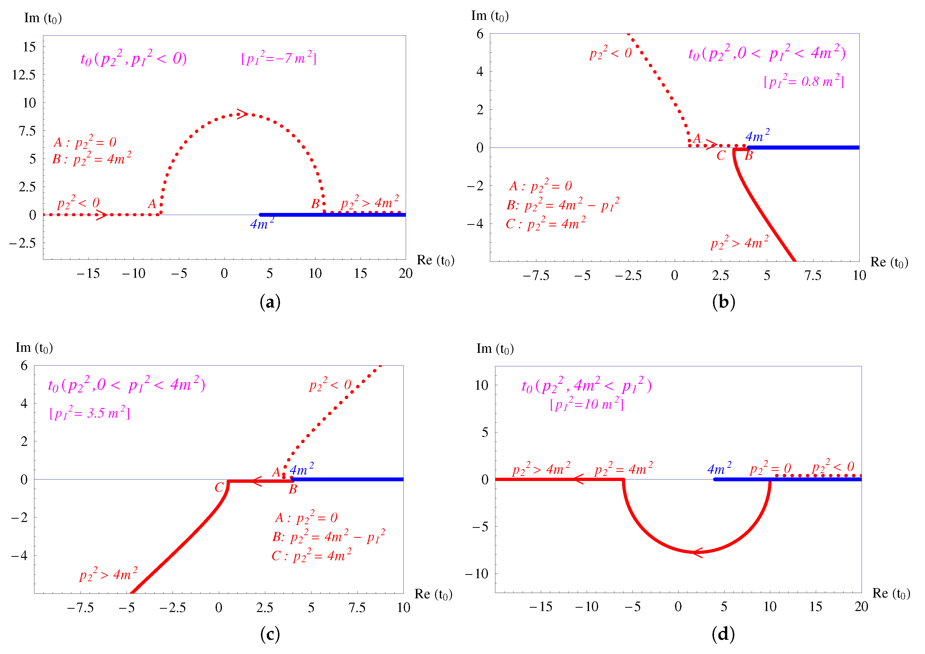
The branch point , treated as the function of at fixed , has a rather cumbersome trajectory on the second sheet of the complex plane, but never appears on the physical sheet (see Figure 2). This means that the motion of this branch point does not influence the single -spectral representation for .
2.3. The Branch Point
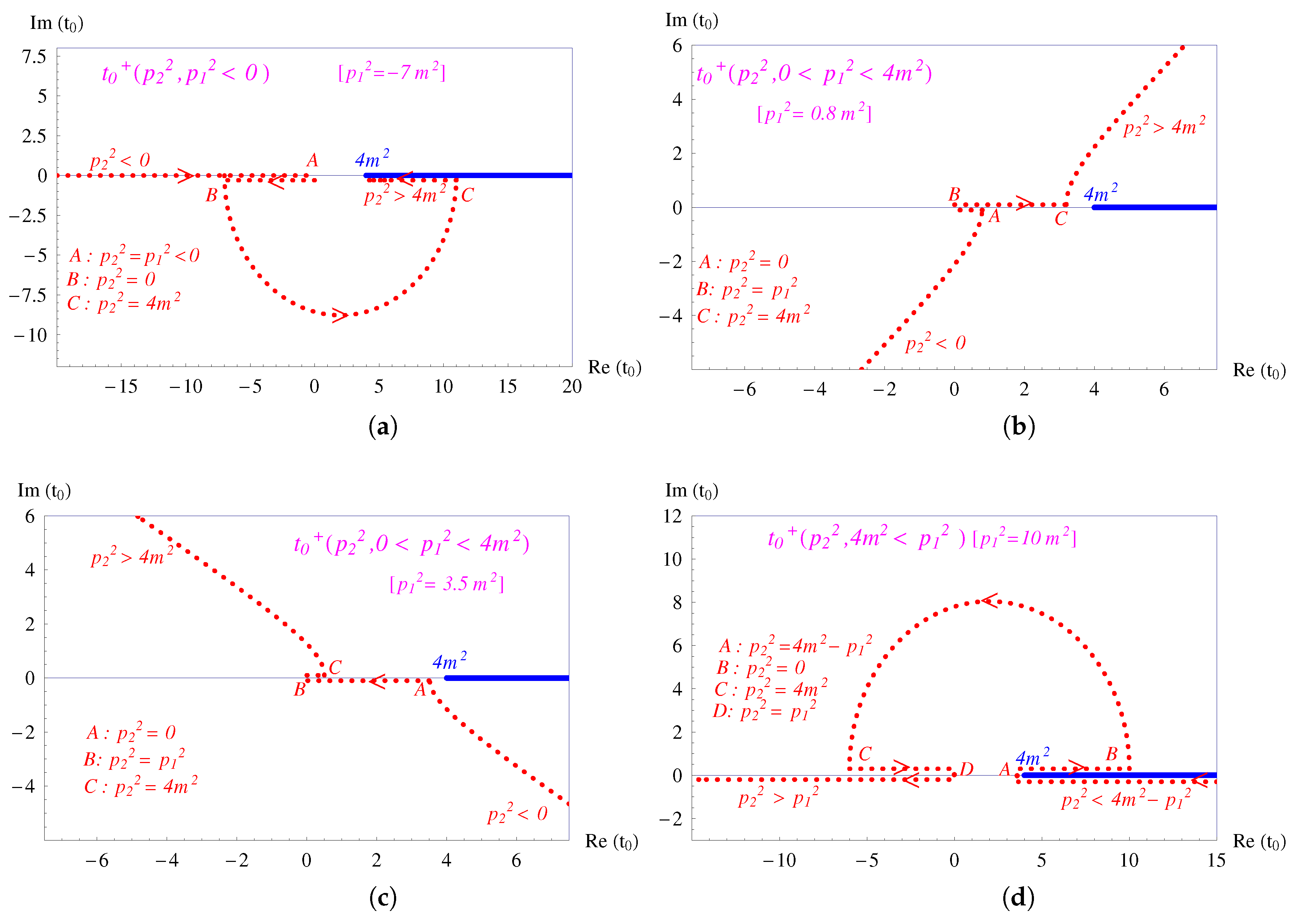
Treated as the function of for a fixed value of , the branch point has its trajectory at on the unphysical sheet of the complex -plane. However, at some value of , it crosses the cut at . Crossing the cut means that the branch point moves onto the physical sheet through this cut. The integration contour in the Cauchi theorem is chosen on the physical sheet of complex variable and embraces (any) region of complex variable , where the function of the complex variable has no singularities. The migration of the branch point onto the physical sheet pushes the integration contour away from the normal threshold and leads to the appearance of a new segment of the -integration on the physical sheet [10,14]. This new segment is called the anomalous cut. The trajectories of vs. for four different fixed values of are shown in Figure 3. The dotted lines denote the segments of the trajectory lying on the unphysical sheet; the solid lines denote those segments that are on the physical sheet.
Therefore, for external momenta satisfying the relation , , , the integration contour in the dispersion representation for the form factor depends on the values of and : the contour should be chosen such that it embraces both branch points: the normal branch point at and the anomalous branch point at .
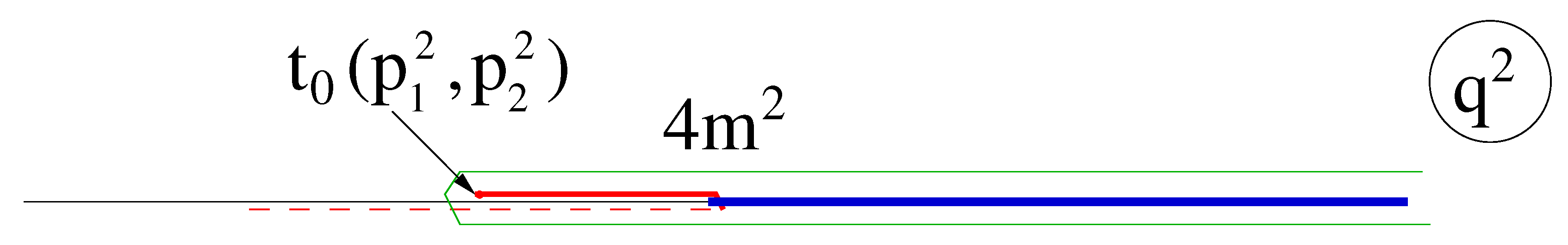
Let us consider the single dispersion representation for the form factor in the region , , and . This case corresponds to the interesting example of a two-particle bound state, and is necessary for considering the nonrelativistic expansion. The corresponding -trajectory is shown in Figure 3. Figure 4 gives the integration contour for this case: this contour may be chosen along the real axis from to . It contains two pieces: the normal part from to and the anomalous part from to .
Let us start with the normal part, which has the form
Notice that the normal spectral density does not vanish at the normal threshold .
The discontinuity of the form factor on the anomalous cut is related to the discontinuity of the function and reads
Therefore, the full spectral density has the form
Clearly, the spectral density given by Equations (11) and (12) is a continuous function for . The spectral representation for the form factor then contains the normal and the anomalous contributions:
For (in case ), the imaginary part of the form factor comes from the anomalous part, while for it comes from the normal part.
2.4. An Illustration for the Case of Equal External Masses
Let us now specify the general formulas given above for the case of the equal “external” masses. We set , and aim at obtaining the dispersion representation for the case . Notice that both and are below the normal thresholds; the latter are located at and . Nevertheless, we shall see that the anomalous threshold in the single dispersion representation in will emerge.
We start with calculating the spectral density in the region , where it is given by Cutkosky rules:
It turns out that this expression is also valid in a broader domain, namely, (see Figure 5a). Performing the analytic continuation in variable from the domain , we obtain the spectral density for the region of interest :
Figure 5b,c shows the cases and , respectively. In the latter case, the normal spectral density does not vanish at the normal threshold . The discontinuity of the form factor on the anomalous cut is related to the discontinuity of the function and reads
Therefore, the full spectral density has the form
The spectral density given by Equations (16) and (17) is a continuous function for (see Figure 5c).
The spectral representation for the form factor reads
It can be also written in the usual form
where contains the normal and the anomalous pieces.
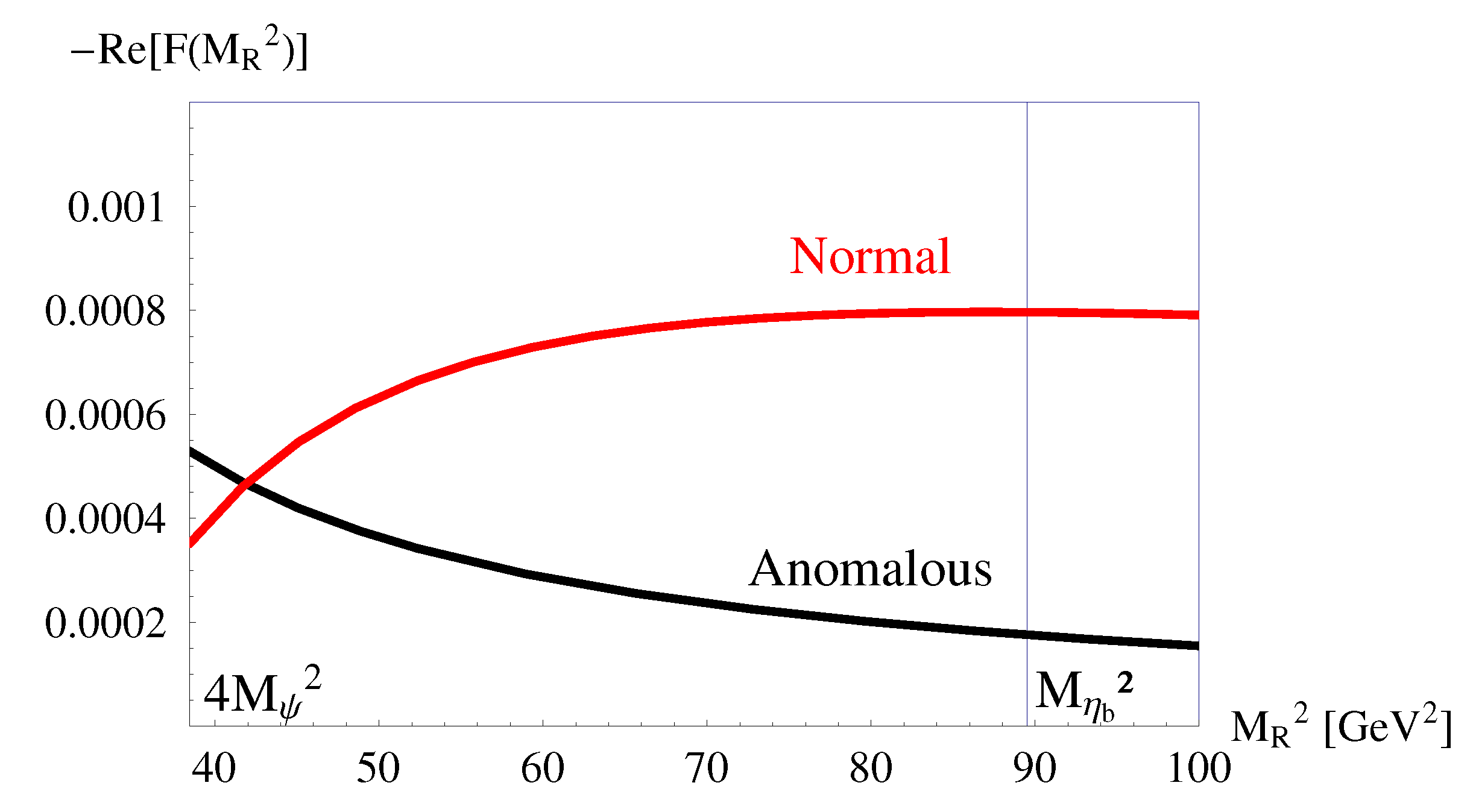
Figure 6 shows the calculated real parts of the normal and the anomalous contributions to the form factor depending on the value of the mass of the decaying resonance .
3. Double Dispersion Representation in and for Particles of Mass m in the Loop
The previous section presented the single dispersion representation in for the triangle diagram with particles of mass m in the loop. For the same triangle diagram, a double dispersion representation in and may be written [15,16,17,18,19].
At , such a double dispersion representation in and has the form:
The double spectral density may be obtained by placing all three particles in the loop on the mass shell and taking the off-shell external momenta , , such that , , and is fixed [15,16]:
Explicitly, one finds
The solution of the -function gives the following allowed intervals for the integration variables and :
where
The final double dispersion representation for the triangle diagram at takes the form (The easiest way to obtain this double dispersion representation is to introduce light-cone variables in the Feynman expression, and to choose the reference frame where (which restricts to ). Then, the integral is easily done, and the remaining y and integrals may be written in the form (21); details can be found in [15,16].)
Notice the relation , which holds for all at : this guarantees that the integration region in always remains above the normal threshold. Clearly, the integration region does not depend on the values of and . It is essential for us is that no anomalous cuts emerge in the double dispersion representation in and for . This makes the double dispersion representation particularly convenient for treating the triangle diagram for values of and above the thresholds. One should just take care about the appearance of the absorptive parts.
4. Double Spectral Representation for the Decay Kinematics
Now, we discuss the triangle diagram with particles of different masses in the loop, , and consider the decay kinematics [13,20,21,22,23]. We have in mind the application to processes corresponding to the overthreshold values and , such as, e.g., the decay. As we have seen in the previous section, the single dispersion representation in is rather complicated for and above the two-particle thresholds already for equal masses in the loop. The situation is much worse for unequal masses in the loop. On the other hand, we shall see that the double spectral representation in and is rather simple for .
We start with the region , where the double dispersion representation has the standard form both for equal and unequal masses in the loop. We then perform the analytic continuation in and observe the appearance of the anomalous contribution in the double spectral representation.
4.1. Transition Form Factor at
For , the double dispersion representation has a form very similar to the case of equal masses [23]:
where
A new feature compared with the case of equal masses in the loop is the appearance of the region , which was absent in the equal-mass case. This region corresponds to the decay of a particle of mass to a particle of mass m with the emission of a particle of mass .
4.2. Transition Form Factors at
The form factor in the region may be obtained by analytic continuation of the expression (26). Let us consider the structure of the singularities of the integrand in Equation (27) in the complex -plane for a fixed real value of in the interval .
The integrand has singularities (branch points) related to the zeros of the function at and . As , these singularities lie on the unphysical sheet. However, as becomes positive, the point may move onto the physical sheet through the cut from to . This happens for values of the variable , with obtained as the solution to the equation . Explicitly, one finds
The trajectory of the point in the complex -plane at fixed vs. is shown in Figure 7. As , for , the integration contour in the complex -plane should be deformed such that it embraces the points and . Respectively, the -integration contour contains the two segments: the normal part from to , and the anomalous part from to . The double spectral density for the anomalous piece is just the discontinuity of the function . It can be easily calculated as follows: Recall the relation . The branch point lies on the unphysical sheet, therefore the function is continuous on the anomalous cut located on the physical sheet. Thus, we have to calculate the discontinuity of the function which is just twice the function itself. As a result, the discontinuity of the function on the anomalous cut is . Finally, the full double spectral density, including the normal and the anomalous pieces, takes the form
The first term in Equation (30) relates to the Landau-type contribution emerging when all intermediate particles go on mass shell, while the second term describes the anomalous contribution.
The result (30) for holds for implying the “external” -integration, and the “internal” -integration. The location of the integration region for this case is shown in Figure 7. Figure 8 gives the integration contour in the complex plane for the opposite integration order.
The final representation for the form factors at takes the form
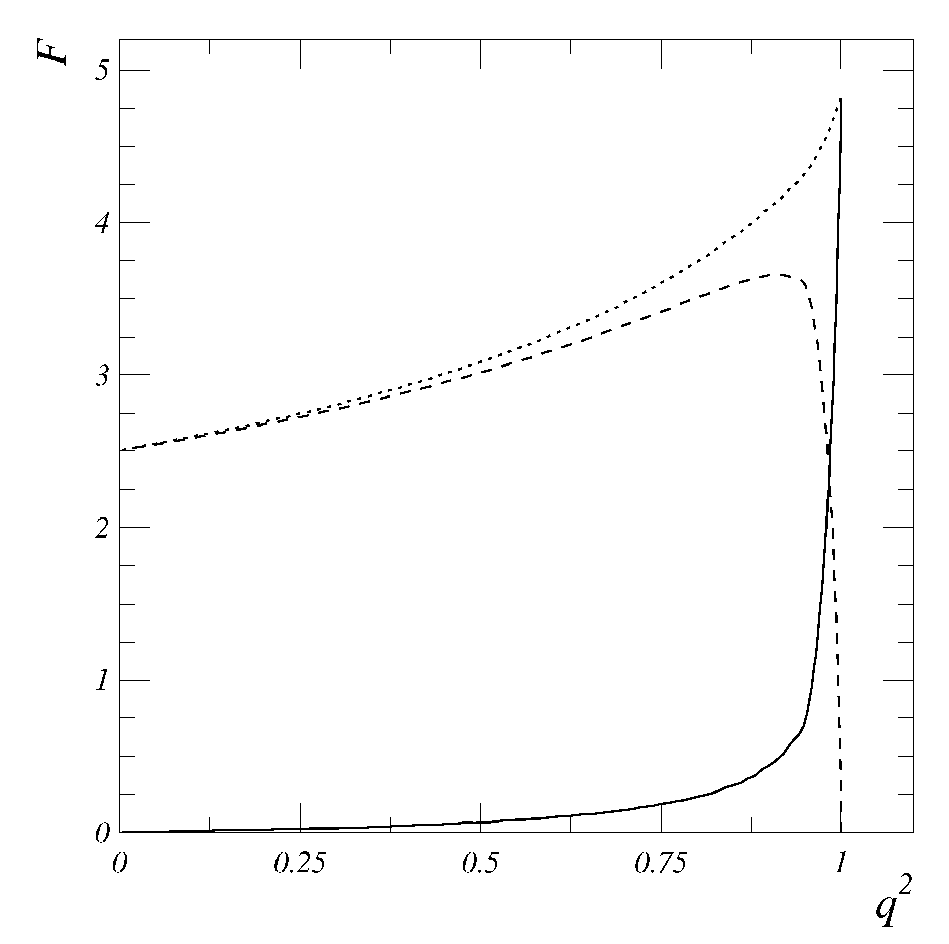
A typical behavior of the anomalous and the normal contributions is plotted in Figure 9: the normal contribution first rises at small positive values of but then falls down steeply and vanishes at zero recoil. The anomalous contribution is zero at , remains small at small , but rises steeply near zero recoil, providing a smooth behavior of the full form factor.
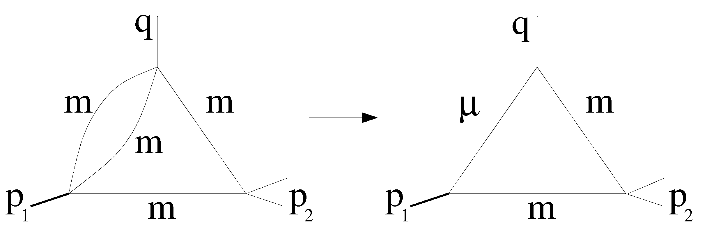
We point out that the representation (31) is particularly suitable for application to processes where and are above two-particle thresholds: in this case, the single spectral representation in becomes extremely complicated, with a nontrivial integration contour in the complex -plane, whereas the double dispersion representation in and has the simple form given above. For values of and above the thresholds, one just has to take into account the appearance of the absorptive parts in the and integrals. A possible application of this representation may be the calculation of the triangle-diagram contribution to the three-body decay [24,25], e.g., to the decay [26,27], Figure 10. In this case, the diagram with the pion loop may be represented as the integral of the triangle diagram considered here, and one obtains the expression for the values , , and . The emerging absorptive parts may then be easily calculated from the double spectral representation. The problem would be technically very involved if one uses the single spectral representation in , as can be seen from the complicated structure of the integration contour in Section 2.
5. Summary and Conclusions
I have presented a detailed analysis of dispersion representations for the triangle diagram, laying main emphasis on the appearance of the anomalous contributions in these representations. These anomalous singularities play an important role in the analysis of physical processes, see, e.g., [28,29,30,31,32,33,34,35,36,37,38,39] and a recent review [40] for details. In some kinematic regions, the properties of the triangle diagram and the amplitudes of the corresponding processes are mainly determined by the anomalous contributions. A message I would like to convey to the reader is that in many cases the double spectral representations in and provide great technical advantages compared to the use of the single representation in . This is clearly the case for and above the thresholds and in the decay region . Several realistic physical cases belong to this class of problems.
Let me highlight a few points presented in this lecture:
The single dispersion representation for the triangle diagram in the variable develops an anomalous threshold, related to a migration of the logarithmic branch point from the unphysical (second) sheet of the Riemann surface onto the physical sheet through the normal -cut. This migration occurs for the specific relationship between the squares of the external momenta and and the masses of the particles propagating in the loop. For instance, for the case , and the particles with mass m in the loop, the anomalous threshold occurs for all , i.e., for the external masses below the unitary thresholds . This means, in particular, that the anomalous thresholds occur for weakly-bound states, when and . In this case, the location of the anomalous threshold in is responsible for the (large) radius of the weakly-bound state.
It should be taken into account that the appearance of the anomalous cut in the single dispersion representation changes the leading singularity of the triangle diagram on the physical sheet:
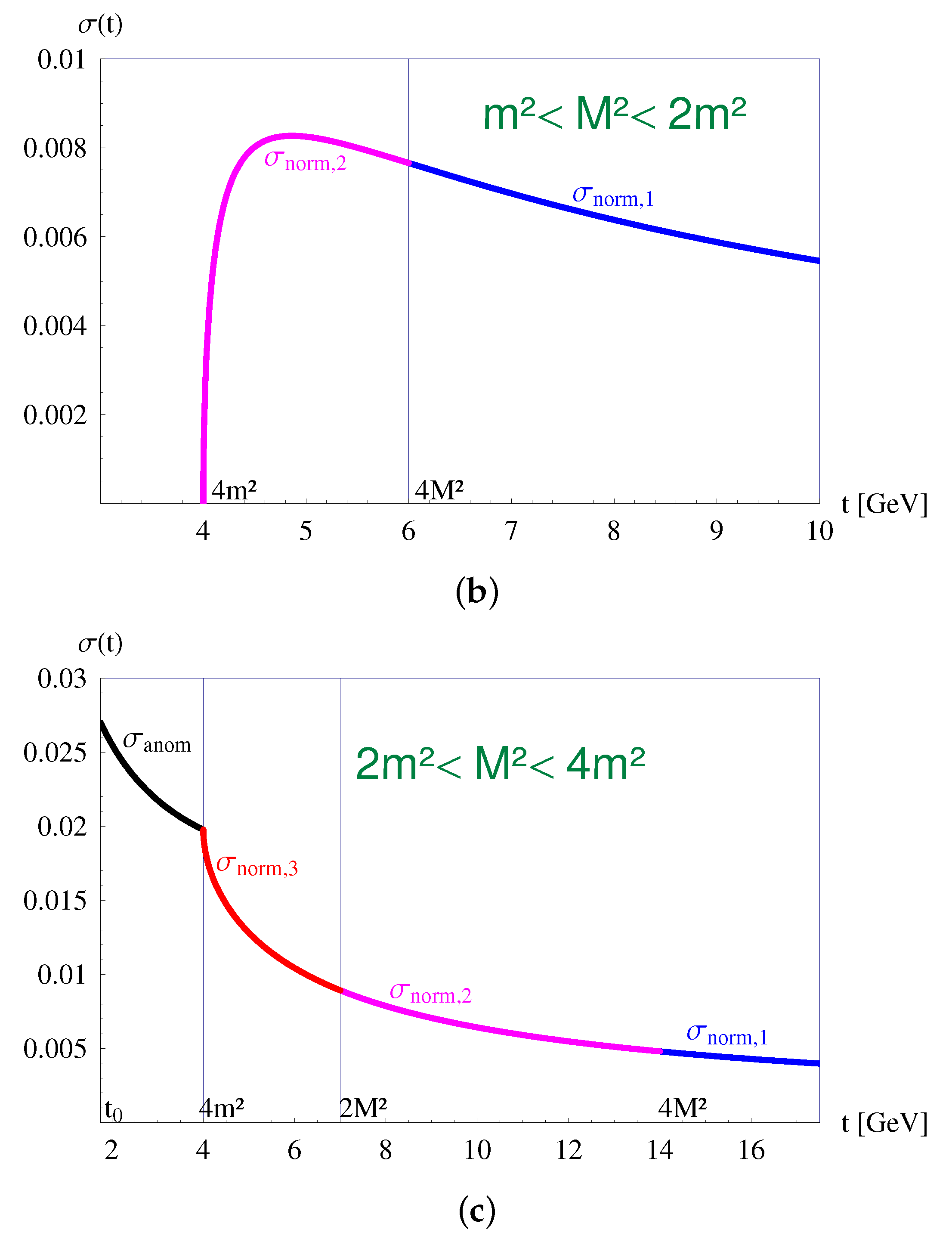
(a) In the “normal” case, , the spectral density of the triangle function has zero at the threshold, (Figure 5a,b), thus yielding the leading singularity of the triangle function.
(b) In the “anomalous” case, , the spectral density of the triangle function does not vanish at the anomalous threshold (Figure 5c), thus yielding the leading singularity. Emphasize that the logarithmic singularity does not emerge on the physical sheet in the “normal” case.
We pointed out that at spacelike momentum transfer q, , and for any values of and , the double dispersion representation in and is particularly simple and contains only the normal cuts. The calculation of the triangle diagram in this case may be easily done for all values of and , including the values above the thresholds and complex values. In the same situation, the single spectral representation in contains, in addition, the anomalous cut, making the application of the single dispersion representation a very involved problem.
For the decay kinematics , the anomalous thresholds and the anomalous cuts emerge in the double dispersion representations in the variables and . In this case, the anomalous threshold in the variable (or ) is absent at but emerges for positive values of . This anomalous threshold in this case lies above the normal unitary threshold at and . The anomalous contribution is small at small positive , but steeply rises when approaches the point . On the contrary, the normal contribution dominates the form factor at small but vanishes at .
In the decay region , the double spectral representation in and provides a very convenient tool for considering processes at and above the thresholds. The application of the single spectral representation in faces in this case severe technical problems.
Acknowledgments
It gives me great pleasure to express my gratitude to Vladimir Anisovich, Wolfgang Lucha, Hagop Sazdjian, and Silvano Simula for collaboration on the problems discussed in this lecture. I would also like to thank the Organizers for creating a friendly and productive atmosphere at this School.
Conflicts of Interest
The author declares no conflict of interest.
References
Karplus, R.; Sommerfeld, C.; Wichman, E. Spectral Representations in Perturbation Theory. I. Vertex Functions. Phys. Rev.1958, 111, 1187. [Google Scholar] [CrossRef]
Landau, L.D. On analytic propertiesn of vertex parts in quantum field theory. Nucl. Phys.1959, 13, 181. [Google Scholar] [CrossRef]
Fronsdal, C.; Norto, R.E. Spectral Representations for Vertex Functions. J. Math. Phys.1964, 5, 100. [Google Scholar] [CrossRef]
Burton, G. Introduction to Dispersion Methods in Field Theory; W. A. Benjamin: NY/Amsterdam, The Netherlands, 1965. [Google Scholar]
Anisovich, V.V.; Kobrinsky, M.N.; Shabelsky, Y.M.; Nyiri, J. Quark Model and High-Energy Collisions; World Scientific: Singapore, 2004. [Google Scholar]
Itzykson, C.; Zuber, J.B. Quantum Field Theory; International Series in Pure and Applied Physics; McGraw-Hill: New York, NY, USA, 1980. [Google Scholar] [CrossRef]
Zwicky, R. A brief Introduction to Dispersion Relations and Analyticity. arXiv2016, arXiv:1610.06090. [Google Scholar]
Lucha, W.; Melikhov, D.; Simula, S. Dispersion representations and anomalous singularities of the triangle diagram. Phys. Rev. D2007, 75, 016001. [Google Scholar] [CrossRef]
Lucha, W.; Melikhov, D.; Sazdjian, H. Tetraquarks and two-meson states at large-Nc. Eur. Phys. J.2017, C77, 866. [Google Scholar] [CrossRef]
Lucha, W.; Melikhov, D.; Sazdjian, H. Tetraquark-adequate QCD sum rules for quark-exchange processes. Phys. Rev.2019, D100, 074029. [Google Scholar] [CrossRef]
Ball, P.; Braun, V.M.; Dosch, H.G. Form-factors of semileptonic D decays from QCD sum rules. Phys. Rev.1991, D44, 3567. [Google Scholar]
Colangelo, G.; Hoferichter, M.; Procura, M.; Stoffer, P. Dispersion relation for hadronic light-by-light scattering: Theoretical foundations. JHEP2015, 1509, 074. [Google Scholar] [CrossRef]
Anisovich, V.V.; Kobrinsky, M.N.; Melikhov, D.I.; Sarantsev, A.V. Ward identities and sum rules for composite systems described in the dispersion relation technique: The Deuteron as a composite two nucleon system. Nucl. Phys.1992, A544, 747. [Google Scholar] [CrossRef]
Anisovich, V.V.; Melikhov, D.I.; Metsch, B.C.; Petry, H.R. The Bethe-Salpeter equation and the dispersion relation technique. Nucl. Phys.1993, A563, 549. [Google Scholar] [CrossRef]
Anisovich, V.; Melikhov, D.; Nikonov, V. Quark Structure of the Pion and Pion Form Factor. Phys. Rev.1995, D52, 5295. [Google Scholar] [CrossRef] [PubMed]
Anisovich, V.; Melikhov, D.; Nikonov, V. Photon-meson transition form factors γπ, γη, and γη′ at low and moderately high Q2. Phys. Rev.1997, D55, 2918. [Google Scholar]
Lucha, W.; Melikhov, D. The γ*γ*→ηc transition form factor. Phys. Rev.2012, D86, 016001. [Google Scholar]
Melikhov, D. Form-factors of meson decays in the relativistic constituent quark model. Phys. Rev.1996, D53, 2460. [Google Scholar] [CrossRef]
Melikhov, D. Heavy quark expansion and universal form-factors in quark model. Phys. Rev.1997, D56, 7089. [Google Scholar] [CrossRef]
Melikhov, D.; Stech, B. Weak form-factors for heavy meson decays: An Update. Phys. Rev.2000, D62, 014006. [Google Scholar] [CrossRef]
Melikhov, D. Dispersion approach to quark binding effects in weak decays of heavy mesons. Eur. Phys. J. Direct2002, 4, 1–54. [Google Scholar] [CrossRef]
Anisovich, V.V.; Anselm, A.A.; Gribov, V.N.; Dyatlov, I.T. Anomalous thresholds and final state interaction. Sov. Phys. JETP1963, 16, 643. [Google Scholar]
Anisovich, V.V.; Anselm, A.A. Theory of Reactions with Production of Three Partciles near Thresholds. Sov. Phys. Uspekhi1966, 9, 117. [Google Scholar] [CrossRef]
Cabibbo, N.; Isidori, G. Pion-pion scattering and the K→3π decay amplitudes. JHEP2005, 503, 021. [Google Scholar] [CrossRef]
Colangelo, G.; Gasser, J.; Kubis, B.; Rusetsky, A. Cusps in K→3π decays. Phys. Lett.2006, B638, 187. [Google Scholar] [CrossRef]
Santorelli, P. Long-distance contributions to the ηb→J/ψJ/ψ decay. Phys. Rev.2008, D77, 074012. [Google Scholar]
Liu, X.-H.; Oka, M.; Zhao, Q. Searching for observable effects induced by anomalous triangle singularities. Phys. Lett.2016, B753, 297. [Google Scholar] [CrossRef]
Hoferichter, M.; Hoid, B.-L.; Kubis, B.; Leupold, S.; Schneider, S.P. Pion-pole contribution to hadronic light-by-light scattering in the anomalous magnetic moment of the muon. Phys. Rev. Lett.2018, 121, 112002. [Google Scholar] [CrossRef]
Hoferichter, M.; Hoid, B.-L.; Kubis, B.; Leupold, S.; Schneider, S.P. Dispersion relation for hadronic light-by-light scattering: Pion pole. JHEP2018, 1810, 141. [Google Scholar] [CrossRef]
Hoferichter, M.; Stoffer, P. Dispersion relations for γ*γ*→ππ: Helicity amplitudes, subtractions, and anomalous thresholds. JHEP2019, 1907, 073. [Google Scholar] [CrossRef]
Szczepaniak, A.P. Dalitz plot distributions in the presence of triangle singularities. Phys. Lett.2016, B757, 61. [Google Scholar] [CrossRef]
Mikhasenko, M. A triangle singularity and the LHCb pentaquarks. arXiv2015, arXiv:1507.06552. [Google Scholar]
Mikhasenko, M.; Ketzer, B.; Sarantsev, A. Nature of the a1(1420). Phys. Rev.2015, D91, 094015. [Google Scholar]
Guo, F.-K.; Meißner, U.-G.; Wang, W.; Yang, Z. How to reveal the exotic nature of the Pc(4450). Phys. Rev.2015, D92, 071502. [Google Scholar]
Liu, X.-H.; Wang, Q.; Zhao, Q. Understanding the newly observed heavy pentaquark candidates. Phys. Lett.2016, B757, 231. [Google Scholar] [CrossRef]
LHCb Collaboration. Observation of a narrow pentaquark state, Pc(4312)+, and of two-peak structure of the Pc(4450)+. Phys. Rev. Lett.2019, 122, 222001. [Google Scholar] [CrossRef]
Guo, F.-K.; Liu, X.-H.; Sakai, S. Threshold cusps and triangle singularities in hadronic reactions. arXiv2019, arXiv:1912.07030. [Google Scholar] [CrossRef]
Figure 1.
The Feynman diagram .
Figure 1.
The Feynman diagram .
Figure 2.
The trajectory of the branch point vs. at a fixed value of in the complex- plane. Dashed lines denote trajectories on the second (unphysical) sheet. (a) []; (b,c) : (b) ; (c) ; (d) []. The normal cut along the real axis for is depicted in blue. It is noteworthy that the branch point always remains on the second (unphysical) sheet of the Riemann surface and never migrates onto the physical sheet. Therefore, does not influence the location of the cut on the physical sheet.
Figure 3.
The trajectory of the branch point vs at a fixed value of in the complex- plane: (a) []: the (dashed line) trajectory lies on the second sheet, and does not appear on the physical sheet; (b,c) [(b): , (c): ]: the trajectory first lies on the second sheet (dashed line), but for moves around the normal-cut branch point through the normal cut onto the physical sheet (solid line); (d) []: for , the trajectory runs on the unphysical sheet, but, at , it comes up to the physical sheet and for travels over this physical sheet. As soon as the branch point appears on the physical sheet, the -integration contour should be modified such that it embraces both the normal cut and the branch point . The normal cut along the real axis for is depicted in blue.
Figure 4.
The integration contour (green) in the complex -plane for , , and : it embraces the anomalous cut (the solid red segment from to ) and the normal cut (blue line from to ). The dotted red line displays the trajectory of the branch point on the unphysical sheet.
Figure 4.
The integration contour (green) in the complex -plane for , , and : it embraces the anomalous cut (the solid red segment from to ) and the normal cut (blue line from to ). The dotted red line displays the trajectory of the branch point on the unphysical sheet.
Figure 5.
The spectral density for different values of m and M. (a) ; (b) ; (c) . (blue line) corresponds to the analytic expression in the first line of Equation (16); (magenta line) corresponds to the analytic expression in the second line of Equation (16); and (red line) corresponds to the analytic expression in the third line of Equation (16). (black line) is given by Equation (17). Notice that, for , plots (a) and (b), the spectral density vanishes at the normal threshold , whereas, in the case , plot (c), the spectral density does not vanish neither at the normal threshold , nor at the anomalous threshold .
Figure 6.
The real part of the normal (red) and of the anomalous (black) contributions to the amplitude vs. . Here, we use the following numbers GeV, GeV, and GeV.
Figure 6.
The real part of the normal (red) and of the anomalous (black) contributions to the amplitude vs. . Here, we use the following numbers GeV, GeV, and GeV.
Figure 7.
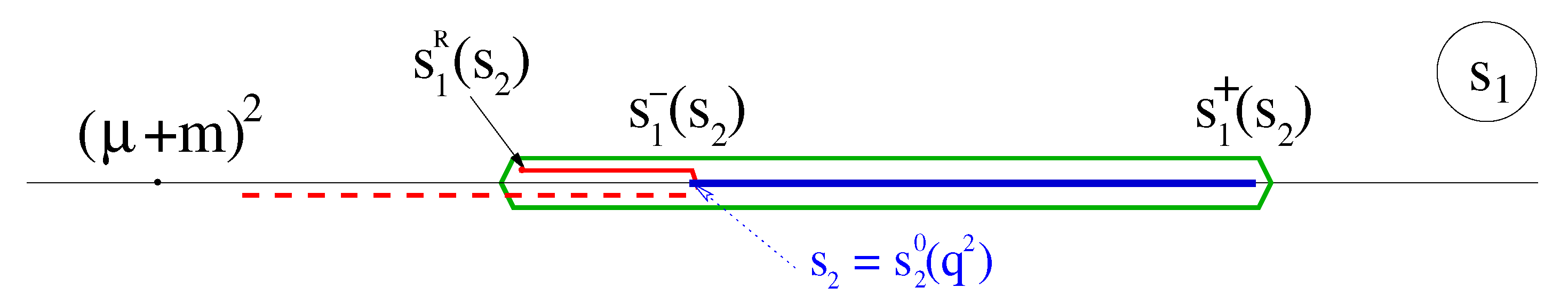
Singularities of the function in the complex plane as a function of for . (This corresponds to the external and the internal integration). The plot shows the trajectory vs at fixed : for , the branch point moves on the unphysical sheet (dashed red line). However, as soon as , travels around the branch point through the normal cut , appears on the physical sheet, and further moves to the left from (solid red line). Respectively, for , the integration contour in the complex -plane may be chosen along the interval . For , however, the contour should embrace the point , and therefore the integration contour (green line) contains two segments: the “anomalous” segment from to (solid red line), and the “normal” segment from to (blue line). The real axis of the variable is shown as black line.
Figure 7.
Singularities of the function in the complex plane as a function of for . (This corresponds to the external and the internal integration). The plot shows the trajectory vs at fixed : for , the branch point moves on the unphysical sheet (dashed red line). However, as soon as , travels around the branch point through the normal cut , appears on the physical sheet, and further moves to the left from (solid red line). Respectively, for , the integration contour in the complex -plane may be chosen along the interval . For , however, the contour should embrace the point , and therefore the integration contour (green line) contains two segments: the “anomalous” segment from to (solid red line), and the “normal” segment from to (blue line). The real axis of the variable is shown as black line.
Figure 8.
Singularities of the function in the complex plane as a function of for . (This corresponds to the external and the internal integration). The trajectory vs at fixed is shown by the red line: for the branch point remains on the unphysical sheet (dashed red line), but, as soon as , it goes onto the physical sheet and moves to the right from the right boundary of the normal cut (solid red line). Respectively, for , the contour should embrace the point , and the integration contour (green line) contains two segments: the “normal” segment from to (blue line) and the “anomalous” segment from to (solid red line). The real axis of the variable is shown as black line.
Figure 9.
A typical behavior of the function vs. for at fixed and . The parameters are chosen such that GeV. Dashed: normal part, solid: anomalous part, dotted: full function (sum of both parts).
Figure 9.
A typical behavior of the function vs. for at fixed and . The parameters are chosen such that GeV. Dashed: normal part, solid: anomalous part, dotted: full function (sum of both parts).
Figure 10.
The triangle-diagram contribution to the amplitude may be reduced to the integral over of the diagram F.
Figure 10.
The triangle-diagram contribution to the amplitude may be reduced to the integral over of the diagram F.
Melikhov, D.
Analytic Properties of Triangle Feynman Diagrams in Quantum Field Theory. Particles2020, 3, 99-113.
https://doi.org/10.3390/particles3010009
AMA Style
Melikhov D.
Analytic Properties of Triangle Feynman Diagrams in Quantum Field Theory. Particles. 2020; 3(1):99-113.
https://doi.org/10.3390/particles3010009
Chicago/Turabian Style
Melikhov, Dmitri.
2020. "Analytic Properties of Triangle Feynman Diagrams in Quantum Field Theory" Particles 3, no. 1: 99-113.
https://doi.org/10.3390/particles3010009
APA Style
Melikhov, D.
(2020). Analytic Properties of Triangle Feynman Diagrams in Quantum Field Theory. Particles, 3(1), 99-113.
https://doi.org/10.3390/particles3010009
Article Metrics
No
No
Article Access Statistics
For more information on the journal statistics, click here.
Multiple requests from the same IP address are counted as one view.
Melikhov, D.
Analytic Properties of Triangle Feynman Diagrams in Quantum Field Theory. Particles2020, 3, 99-113.
https://doi.org/10.3390/particles3010009
AMA Style
Melikhov D.
Analytic Properties of Triangle Feynman Diagrams in Quantum Field Theory. Particles. 2020; 3(1):99-113.
https://doi.org/10.3390/particles3010009
Chicago/Turabian Style
Melikhov, Dmitri.
2020. "Analytic Properties of Triangle Feynman Diagrams in Quantum Field Theory" Particles 3, no. 1: 99-113.
https://doi.org/10.3390/particles3010009
APA Style
Melikhov, D.
(2020). Analytic Properties of Triangle Feynman Diagrams in Quantum Field Theory. Particles, 3(1), 99-113.
https://doi.org/10.3390/particles3010009


