Remaining Useful Life Prediction Method Enhanced by Data Augmentation and Similarity Fusion

Abstract

Precise prediction of the remaining useful life (RUL) of rolling bearings is crucial for ensuring the smooth functioning of machinery and minimizing maintenance costs. The time-domain features can reflect the degenerative state of the bearings and reduce the impact of random noise present in the original signal, which is often used for life prediction. However, obtaining ideal training data for RUL prediction is challenging. Thus, this paper presents a bearing RUL prediction method based on unsupervised learning sample augmentation, establishes a VAE-GAN model, and expands the time-domain features that are calculated based on the original vibration signals. By combining the advantages of VAE and GAN in data generation, the generated data can better represent the degradation state of the bearings. The original data and generated data are mixed to realize data augmentation. At the same time, the dynamic time warping (DTW) algorithm is introduced to measure the similarity of the dataset, establishing the mapping relationship between the training set and target sequence, thereby enhancing the prediction accuracy of supervised learning. Experiments employing the XJTU-SY rolling element bearing accelerated life test dataset, IMS dataset, and pantograph data indicate that the proposed method yields high accuracy in bearing RUL prediction.

1. Introduction

Rolling bearings are vital components of rotating equipment. Their failure can have severe consequences, including the failure of the entire mechanical system. Such failures pose a significant risk of safety accidents during actual production, leading to unpredictable outcomes [1,2]. Therefore, the development of remaining useful life (RUL) technologies provides a strong assurance for the reliable functioning of equipment [3], which can help engineers carry out timely maintenance and replacement, reduce economic losses, and improve the economic benefits of enterprises.

In recent years, the data-driven method based on supervised learning is very popular in the field of equipment failure prediction, which mainly includes the construction of health indicators (HIs) and RUL prediction. The constructed HIs and corresponding target labels are employed to train the prediction model for subsequent test set verification. Therefore, the construction of appropriate HIs plays a crucial part in RUL prediction. Based on varying construction strategies for HIs, existing methods are primarily categorized into two approaches, namely direct HI (PHI) and indirect HI (VHI). PHI is typically obtained by employing various techniques in the original signal analysis or signal processing, also referred to as physical HIs. The spectral entropy based on multi-scale morphological decomposition employed by Wang Bing et al. [4] and the binary multi-scale entropy adopted by Li Hongru et al. [5] are HIs obtained using statistical methods from the original signals. Gebraeel et al. [6] extracted the average amplitudes and harmonics to serve as PHI. VHI is generally constructed using fusion or dimensionality reduction methods, because it does not have actual physical significance. Wang et al. [7] fused 12 time-domain features into a new health index using Mahalanobis distance. Xia et al. [8] used spectral regression technology to reduce the dimensionality of fault features in time-domain, frequency-domain, and time–frequency domain extracted from rolling bearing vibration signals to derive new features. However, the time-domain characteristics (PHI) relevant to the degradation trend calculated by the bearings’ original signal are limited (it is theoretically believed that rolling bearings are relatively smooth in the initial stage of degradation, and sharply degenerate near the end of the bearings’ lifespan, and the time-domain features appear relatively drastic in terms of fluctuations), so directly predicting the RUL for bearings lacks high accuracy. Data augmentation aims to address these challenges by generating additional data and effectively employing several frequently employed methods, such as noise injection and data augmentation (expanding or shrinking the dataset) [9], so as to meet the process of predictive model training and verification.

The existing generation models based on machine learning mainly include variational autoencoder (VAE) [10] and generative adversarial network (GAN) [11]. Among them, GAN research has been widely concerned and has found wide applications in applied in stock prediction, image generation, and other fields. Due to its excellent performance and powerful data generation capacity, GAN research has been widely used. It also currently plays a huge role in data generation that generates high-quality, diverse time series. In the domain of prognostics and health management (PHM), Liu et al. [12] proposed an optimized GAN with stable model gradient change and effectively utilized it for machine fault diagnosis. Lu et al. [13] introduced a predictive model for bearing faults that combines GAN and LSTM. Lei et al. [14] utilized the time-domain features as the original data for the GAN and used support vector regression (SVR) and radial basis function neural network (RBFNN) to perform RUL prediction on the amplified data. Numerous studies have shown that data augmentation using GAN outperforms traditional methods, leading to notable enhancements in model performance. For instance, Frid-Adar et al. [15] showed that synthetic data generated using GAN improved classification accuracy from 78.6% to 85.7% compared to affine augmentation. Due to the gradient explosion, gradient disappearance, and other conditions in the practical application of GAN, the generated sample quality is poor, and to address the issue of poor sample quality, it is essential to create a substantial number of samples, which is difficult to achieve the expected goal [16]. In order to build a more comprehensive generative model and develop the generative learning of VAE and GAN, Larsen et al. [17] integrated the two models of VAE and GAN, proposed VAE-GAN, and applied it to face image recognition. Wang et al. [18] proposed a data enhancement method named PVAEGAN, which achieved good fault diagnosis effect by generating a limited quantity of failure data. Considering the advantages of VAE-GAN in the above fields, this paper applies VAE-GAN to sample generation of time series to acquire high-quality time series data set.

In supervised training, the training set and corresponding target labels are fed into the prediction model, with the goal for the model to learn the mapping relationship between them. To evaluate the model’s training effectiveness, test set data are fed into the trained predictive model to derive the forecasted outcome. The training and test sets originate from distinct degradation processes, resulting in lower model prediction accuracy. Typically, we consider the correlation between training sets, and leverage the intrinsic correlation within the training set to assign weights to its data, thereby constructing a novel time series feature for RUL prediction. Nie et al. [19] constructed similarity features by calculating Pearson’s correlation coefficients between time series of features in time-domain and frequency-domain and corresponding time vectors. Hou et al. [20] applied weights to the training set’s RUL, contingent upon the similarity between the training and test sets during the degradation phase, thereby acquiring a similar RUL for the test set to facilitate network training. The DTW algorithm is employed to measure the similarity between time series. It can accurately describe the similarity and difference of time series by stretching, aligning, and warping the time series. Nguyen et al. [21] used the DTW algorithm to calculate the similarity between time series and carry out state matching. Compared with Euclidean distance, it calculated time series more accurately. Experimental findings indicate that utilizing similarity to enhance the predictive accuracy of the model is effective. Therefore, this paper proposes a time series data generation method based on VAE-GAN. By combining the advantages of VAE and GAN in sample generation, the function of data augmentation and data expansion is realized while retaining the original data features and distribution. Moreover, an adaptive time series feature construction method is proposed, and the DTW distance of the training set and target sequence is calculated for similarity evaluation. According to the similarity between the two sets, the enhanced training set data are weighted and fused to construct a DTW weighted feature to enhance the predictive accuracy of supervised learning models.

This paper aims to predict the RUL of rolling bearings, utilizing a similarity weighting approach that combines VAE-GAN and DTW, which is depicted in Figure 1. Firstly, time-domain features are extracted from the bearings’ horizontal vibration signals. Subsequently, the characteristic time-domain features are manually selected and input into the VAE-GAN network. Combining the advantages of VAE and GAN in sample generation, high-quality generated data are obtained. The augmented training set is obtained by mixing generated data and the original data, and then the augmented training set is matched with the target sequence data by DTW similarity to obtain the weighted fusion data. The CNN-LSTM network is trained by the DTW weighted fusion augmented data, and finally the trained prediction model is utilized to obtain RUL predictions using the test set as input. In this paper, the efficacy of the approach is validated via experimental analysis employing the XJTU-SY rolling element bearing accelerated life test dataset. The following outlines the primary contributions of this paper:

(1)

A feature generation method based on VAE-GAN is proposed, which effectively solves the issue of limited capability of original bearing signal to represent degraded state and insufficient effective time-domain features. The generated features are of higher quality and capture more adequate degradation information than the real data.

(2)

In supervised learning, the mapping between the training set and the test set is often unknown. To address this challenge, this study incorporates DTW similarity weighting to match the similarity between training data and target sequence, thereby enhancing the accuracy of bearing RUL prediction.

(3)

The efficacy of the proposed method is confirmed by conducting experiments on public datasets. By combining data augmentation and similarity weighting, a more comprehensive understanding of degradation patterns can be achieved, leading to enhanced prediction performance and accuracy.

The remainder of this paper is organized as follows. In Section 2, a concise review of the foundational theory is described. In Section 3, the basic theory of VAE-GAN data augmentation and similarity fusion with DTW distance is introduced. In Section 4, the evaluation of the generated data quality and the confirmation of the proposed method’s effectiveness are conducted using the XJTU-SY rolling element bearing accelerated life test dataset, and the relevant comparative tests are carried out. Section 5 gives the conclusion.

2. Foundational Theory

2.1. Variational Autoencoder (VAE)

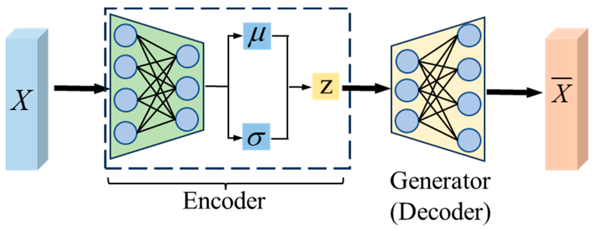
VAE, a variant of the autoencoder, is a neural network that combines probabilistic statistics and deep learning, and its structure is shown in Figure 2. It can be divided into encoder and decoder. Encoder learns the distribution of raw data, converts the original input X into two vectors, one represents the mean vector μ and the other represents the standard deviation vector σ of the distribution. Subsequently, samples are drawn from the sample space defined by the two vectors, and the resulting sample Z, obtained as Z = E(X), is used as the Input for the generator. Nevertheless, training the two values becomes challenging due to the intrinsic randomness of the samples, so the reparameterization technic is utilized to define Z as Equation (1), so that the randomness of the sample will be transferred to ε. The decoder network then restores the hidden variable Z to an approximate reconstructed data.

$${\rm Z}=\mu +\sigma \odot \epsilon$$

(1)

where ε is the auxiliary noise variable from the normal distribution N (0,I).

When real samples are known, the principal objective of the generative model is to capture and learn the underlying data distribution P(X) of this set of data according to the real samples, and samples according to the learned distribution, so as to obtain all possible distributions in line with this set of data.

Because VAE allows potentially complex priors to be set, powerful potential representations of the data can be learned.

2.2. Generative Adversarial Network (GAN)

GAN is a well-known generative algorithm model that consists of two main components, namely the generator model and the discriminator model. The core concept of GAN is to train generators to generate ideal data through the mutual game between generator and discriminator to form an antagonistic loss. The generator aims to closely align the distribution of the generated samples with that of the training samples, while the discriminator evaluates whether a sample is real, or a fake one produced by the generator. The goal of GAN is to use random noise z to train the generator network, so that the generated samples closely resemble real samples, and the discriminator network calculates the probability that the input samples are from the real samples. The framework of the GAN is illustrated in Figure 3:

2.3. Dynamic Time Warping (DTW) Algorithm

The DTW algorithm [22] can reflect the fluctuation trend among bearing vibration signal sequences and has high sensitivity to the fluctuation trend among different vibration signal sequences. Its basic idea is to regularize the time axis by the numerical similarity of the time series, and then find the optimal correspondence between these two temporal sequences. Thus, the DTW distance is utilized to qualify the similarity of the vibration signal sequences in this paper, if the DTW distance of two vibration signals is smaller, it means that the similarity between them is higher, and there is a certain mapping relation between the two sequences.

The DTW distance utilizes the dynamic regularization Idea to adjust the correspondence between the elements of two vibration signal sequences at different times to find an optimal bending trajectory that minimizes the distance between two vibration signal sequences along that path.

Let there be two one-dimensional signal sequences X and Y, X = [x₁, x₂,…, x_r,…, x_R]{1 ≤ r ≤ R} and Y = [y₁, y₂,…, y_s,…, y_S]{1 ≤ s ≤ S}, where r and s are the lengths of X and Y, respectively, an r*s matrix grid is constructed and the matrix elements (r,s) denote the distances between the points x_r and y_s.

The distance between two sequence matches is the distance d_k(r,s) weighted sum:

$$\left\{\begin{array}{l}D(X,Y)={\displaystyle \sum _{k=1}^K{d}_k(r,s)}\\ d(r,s)=\left|x_r-y_s\right|\end{array}\right.$$

(2)

To ensure that the resulting path A is a globally optimal regularized path, the following three constraints must be satisfied: (1) Scope constraints: the beginning position must be (1,1), the end position must be (R,S), to have a beginning and an end; (2) Monotonicity: the path to maintain the time order monotonous non-decreasing, the slope cannot be too small or too large, can be limited to 0.5~2 range; (3) Continuity: r and s can only increase sequentially by 0 or 1, i.e., the point after (r,s) must be (r + 1,s), (r,s + 1) or (r + 1,s + 1).

The path with the minimum cumulative distance is the optimal regularized path, and there is one and only one of them, and the recursive formula for the DTW distance can be found according to Equation (2) and the constraints:

$$D(X,Y)=d(R,S)+min\left\{\begin{array}{l}D(R-1,S-1)\\ D(R,S-1)\\ D(R-1,S)\end{array}\right.$$

(3)

3. Proposed Method

3.1. Data Generation Based on VAE-GAN

3.1.1. Theoretical Illustration

In this paper, VAE-GAN is employed to generate additional time-domain feature curves from bearing vibration signals with characterization. This approach aims to enhance the availability of time series curves for further analysis. The VAE-GAN model incorporates the feature coding component of real data into the GAN and replaces the random noise input in the GAN with the coding result of the VAE, which avoids the situation where the original GAN has no way of deciding which random noise can be used to generate the needed samples and reduces the problem of unstable generated data.

Compared with other generative networks, VAE is able to learn the latent representation of the data, and by leveraging the dimensionality reduction capability of VAE and extracting hierarchical hidden layer information, the generated curves can closely approximate the real feature curves, thus VAE is utilized as a feature generator. VAE consists of two processes, encoding and decoding, the encoding process transforms the original data into hidden variables. The decoding process is to reduce the hidden variables Z to the reconstructed data and the decoder also serves as the generator for the GAN. Where, the encoder, decoder and discriminator all consist of fully connected layers using a Relu activation function to prevent the generated signal from being negative. The discriminator will discriminate the true/false input data from the real data and the output of the generator, so the final layer utilizes a sigmoid activation function and outputs the discriminative probability to obtain the true/false evaluation.

The training of VAE-GAN involves training two key components, which are the discriminator and the generator. The model leverages binary cross entropy (BCE) as its loss function and utilizes Adadelta for loss optimization in unsupervised training. The training process of VAE-GAN is as follows, (1) the extracted original time-domain feature signals are used as the original samples, which are input into the encoder to determine the hidden variable Z. Then, Z is input into the decoder (generator), and the samples are generated by the decoder. In this process, the VAE reconstructs the generated samples by modeling and learning the underlying distribution of the original data; (2) Set labels for the generated samples and original samples, the label corresponding to the generated samples is 0 and the label corresponding to the original samples is 1. The original samples and the generated samples are superimposed, and the true/false labels are superimposed, then they are fed into the discriminator for training; (3) Freeze the parameters of the discriminator and train the generator using GAN so that the samples generated by the generator can be recognized as true data by the discriminator; (4) Unfreezing the parameters of discriminator; (5) Train the discriminator and generator in a loop until both losses are stabilized and output the generated data. The generator G and the discriminator D form a binary minima–maxima game, in which G endeavors to learn the real data distribution to deceive D, and D is trained to determine the veracity of the output generated by G. To fulfill the aforementioned objective, D is trained to maximize the logarithm of D(x) and the parameters of G are adjusted to minimize the logarithm of (l – D(G(z)). The overall adversarial loss is defined as:

$$\underset{G}{min}\underset{D}{max}V(D,G)=E_{x~p_{r(x)}}\left[logD(x)\right]+E_{z~p_{G(z)}}[log(1-D(G(z)))]$$

(4)

where z symbolizes the input noise, x symbolizes the real data, $p_{r(x)}$ symbolizes the sample distribution of the real data, $p_{G(z)}$ symbolizes the sample distribution of the data generated by the generator, and G(z) symbolizes the sample of the data generated by the generator, D(x) symbolizes the probability distribution representing the probability that x is categorized as real data instead of generated data.

3.1.2. Generated Data Assessment

Authenticity Assessment

Once the samples are generated, the initial focus is on examining the correlation or relationship between the generated samples and the original samples, which determines whether the generated samples are true and reliable. The degree of correlation between aleatory variables can be measured by the Pearson’s correlation coefficient, which can be considered as the cosine of the angle between two correlated variables [23]. Pearson’s correlation coefficient was introduced by Karl Pearson and its value lies within the interval [−1, 1]. The value of Pearson’s correlation coefficient is −1 when two variables have a perfectly negative correlation; Pearson’s correlation coefficient has a value of 0 when the two variables are perfectly uncorrelated, and a value of 1 when the two variables are perfectly positively correlated. In this paper, Pearson’s correlation coefficient heat map is utilized to visualize the correlation between the generated data and the original data, a higher value of the correlation coefficient indicates a stronger correlation between the generated features and the original features.

Comprehensiveness Assessment

This study employs time-domain features derived from horizontal vibration signals as the key feature parameters. It is essential to assess whether the temporal evolution of these features follows the degradation process of the bearings, and to select the features whose change process as a whole shows a gradual increasing trend. That is, the change in the early stage of the degradation is relatively smooth, and the change in the late stage is more drastic, and we believe that these features should have good monotonic degradation trend, and they are used as the input samples for the generation of the model. The three evaluation indicators of temporal correlation, monotonicity, and robustness play a positive role in the quantitative evaluation of bearing signal features, and a good feature parameter should have good monotonicity, temporal correlation and anti-interference ability. Therefore, the generated samples are evaluated based on the comprehensive evaluation indicators of monotonicity, correlation, and robustness to determine whether the generated model plays a certain data augmentation effect.

Monotonicity measures whether the changes in the data conform to a gradually increasing or decreasing trend, greater monotonicity represents better monotonicity of the data, and we expect data highly responsive to the degradation process to exhibit a favorable monotonic degradation trend [24]; correlation quantifies the relationship between the feature parameter and the duration of operation, a higher correlation indicates a stronger linear relationship between the feature parameter and time; robustness responds to the degree of tolerance of the model to the data, the greater the monotonicity, indicating that the features can better resist external disturbances such as noise, the more the center degradation features can remain stable.

The generative features are evaluated using a composite metric [25] consisting of correlation, monotonicity, and robustness, where the equations for monotonicity, correlation, and robustness are presented in Equations (5)–(7), respectively:

$$Mon=\frac{\left|Ndf>0-Ndf<0\right|}{S-1}$$

(5)

$$Corr(f_t,t)=\frac{\left|{\displaystyle \sum _{i=1}^S\left(f_s-f_a\right)}\left(t_s-t_a\right)\right|}{\sqrt{{\displaystyle \sum _{i=1}^S{\left(f_s-f_a\right)}^2}}\sqrt{{\displaystyle \sum _{i=1}^S{\left(t_s-t_a\right)}^2}}}$$

(6)

$$Rob=median(|f_s-f_m|)$$

(7)

where Ndf represents the number of df, S represents the number of time series feature points, f represents the time series features of the bearing, df represents the differentiation, f_a denotes the average value of the feature parameter f, t_s represents the value of time t at the moment s, t_a denotes the average value of time t. Median denotes finding the median, and f_m represents the median of the feature parameter under the entire time sequence.

0 ≤ Mon ≤ 1, the larger Mon represents the better monotonicity of the feature parameter. 0 ≤ Corr ≤ 1, the larger Corr represents the better linear correlation between the feature parameter and the time. 0 ≤ Rob ≤ 1, the larger Rob represents the better ability of the feature parameter to resist interference.

The monotonicity, correlation, and robustness are summed, and this metrics is named CI, as in Equation (8), and the generated samples are evaluated by this value. A higher value indicates stronger validity of the generative features in the life prediction generated by the generative model.

$$CI=Mon+Corr+Rob$$

(8)

3.2. Data Augmentation and Fusion

In this paper, RUL prediction is carried out in two steps. Firstly, the augmented data are utilized as the training data, which directly serves as input for the prediction network to verify the effectiveness of data augmentation. Subsequently, the data fused through similarity weighting of the augmented set serves as the training dataset, demonstrating the DTW algorithm’s advantages in weighted fusion of augmented data.

3.2.1. Data Augmentation

After the extraction of time-domain features, few time-domain features were found to be closely related to the bearing degradation trend, so the selected time-domain features were input into the VAE-GAN model for sample generation, and then the original and generated samples were mixed as augmented data to train the prediction model. Augmented data solve the problem of insufficient effective feature parameters and improves the ability to characterize the degraded state of bearings. On the other hand, the mixed data contain richer degradation information compared to the original data, leading to improved prediction accuracy of RUL.

3.2.2. Data Fusion

After the generated data are obtained, the augmented data are weighted and fused, and the distance-weighted features are obtained according to the similarity between the features, which reduces the complexity of the network modeling operation. Since the DTW algorithm has advantages in calculating the similarity between time series, this paper uses the DTW distance as the similarity measure to calculate the DTW distance between the data in each column of the augmented data and the target sequence (where the target sequence is the non-test set sequence data under the same working conditions). The greater the distance, the smaller the similarity. Therefore, weights are assigned to each column of the augmented data, and then the data of each column are multiplied with its own weight and then summed to obtain the weighted fused data, that is, the new training set data. The DTW algorithm uses the learning potential of the network and the similarity matching between the training sequence and the target sequence to refine the training set data by weighting. This strategy aims to make full use of the degradation information contained in the training set data to improve the prediction accuracy of the RUL prediction model. The fusion process is shown in equation (9).

$$Weighted data={\displaystyle \sum _{i=1}^H\left(\left[({\displaystyle \sum _{i=1}^H{w}_{{ }_i}})/w_{{ }_i}\right]A{D}_i\right)}$$

(9)

where AD_i represents a specific column of data within the augmented training set, w_i denotes the DTW distance between a column of data in the training set and the target data, H denotes the number of columns of data. The weight of each column of data in the training set is the inverse of the weight of the DTW distance between it and the target data among all distances.

3.3. RUL Prediction

To further exemplify the effectiveness of the VAE-GAN augmented dataset, the augmented introduced in Section 3.2.1 and the fusion data introduced in Section 3.2.2 and the corresponding degraded labels were input into the CNN-LSTM prediction model for network training, respectively, after that the trained network is applied to the test data to make predictions, yielding the RUL prediction results. Here, the degradation stage is divided by the First Predicting Time (FPT) detection method, in the stage of normal operation, its indicators will exhibit minimal changes [26], the health state does not change, so the data label before the degradation point is set to 1, from the beginning of the degradation point to the complete failure of the bearings from 1 to 0, the degradation stage is labeled as:

$$y=1-\frac{t_n-t_p}{t_a-t_p},t_n\ge t_p$$

(10)

where $t_n$ is the present degradation time, $t_p$ is the time of beginning degradation, and $t_a$ is the total running time.

The prediction results were accessed using two evaluation indicators, root mean square error (RMSE) and R-squared value (R²-SCORE), as shown in Equations (11) and (12).

$$RMSE=\sqrt{\frac{1}{S}{{\displaystyle \sum _{i=1}^S\left(y_s^{*}-y_s\right)}}^2}$$

(11)

$$R^2-SCORE=1-\frac{{{\displaystyle \sum _{i=1}^S\left(y_s-y_s^{*}\right)}}^2}{{{\displaystyle \sum _{i=1}^S\left(y_s-y_a\right)}}^2}$$

(12)

where, $y_s^{*}$ denotes the predicted lifetime at time s, $y_s$ denotes the true lifetime at time s, $y_a$ denotes the mean value of the true lifetime $y_s$, and S denotes the sample size in the test set.

A smaller Root Mean Square Error (RMSE) indicates a smaller prediction error and signifies better model performance. A higher R²-SCORE indicates greater prediction accuracy.

4. Experimental Validation and Analysis

4.1. Data Description

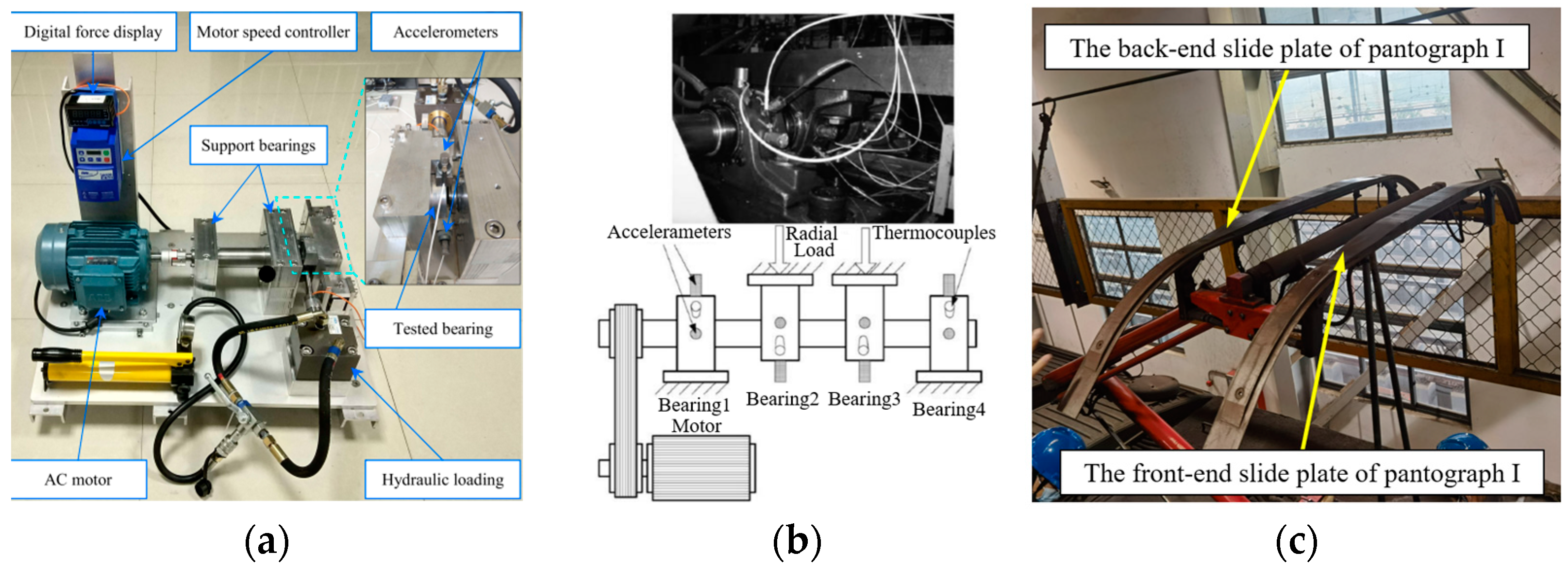
For experimental validation, this paper utilizes the XJTU-SY rolling element bearing accelerated life test dataset [27] and NASA IMS dataset, which are respectively provided by the School of Mechanical Engineering at Xi’an Jiaotong University and NSFI/UCR intelligent maintenance system center. The test bed’s structure is depicted in Figure 4a,b. The two datasets respectively contain accelerated degradation experimental data of 15 and 12 bearings under three working conditions. The sampling frequencies of vibration signals are 25.6 kHz and 20 kHz respectively. The sampling times are 1.28 s every 1 min and 1.024 s every 10 min, respectively. In addition, the wear data of pantograph slide plates of urban rail vehicles in engineering practice were also selected for experimental validation. The dataset contains the pantograph wear degradation data of five urban rail vehicles (Train No. 01037, Train No. 01038, Train No. 01039, Train No. 01040, Train No. 01041, respectively). Each pantograph has two data acquisition locations, the front slide and the rear slide, as shown in Figure 4c, and there are two pantographs per urban rail vehicle, indicating 4 acquisition positions per train.

In this experiment of XJTU-SY bearing dataset, prediction tasks were set, respectively, under each working condition, and details of the test setting were shown in

Table 1. XJTU-SY bearing dataset.

Operating Condition	Number	Training Set	Test Set
2100 r/min, 12 kN	1	Bearing A2, Bearing A3	Bearing A1
	2		Bearing A4
	3		Bearing A5
2250 r/min, 11 kN	4	Bearing B2, Bearing B4, Bearing B5	Bearing B1
	5		Bearing B3
2400 r/min, 10 kN	6	Bearing C1, Bearing C5	Bearing C2
	7		Bearing C3
	8		Bearing C4

. In the experiment of IMS dataset, Bearing B1, Bearing B2, Bearing B3, and Bearing B4 in “2nd_test” of the IMS dataset are selected as the experimental data. Bearing B1 and B3 are selected as the training set. Bearing B2 and B4 are selected as the test set. The training set of pantograph data is the residual thickness of the skateboards at four positions of train 01038, the test data are the pantograph data at the second position of 01037 (referred to as 37B) and the fourth position of 01039 (referred to as 39D), respectively.

4.2. Data Processing

In many scenarios, features extracted from the original signals exhibit variations in scale. Therefore, normalizing and mapping the statistical features extracted from vibration signals to specific equal intervals is essential. The normalization process can eliminate the influence of the scale between the variables, which improves the ease of operation and retains the physical meaning of the data, which can speed up the convergence of the network when conducting RUL prediction and improve the prediction accuracy of the network. In this study, min–max normalization is utilized, and the principle is given in Equation (13).

$$x^{\wedge }=\frac{x-x_l}{x_u-x_l}$$

(13)

where, x = {x₁, x₂,..., x_n} are the vibration data obtained from each sampling, x_l denotes the lowest and x_u denotes the highest values of x, respectively, x^{^} is the normalized data.

4.3. Feature Processing

4.3.1. Feature Extraction and Selection

The 12 time-domain features of the bearings, including mean value, peak value, mean square value, variance, root mean square amplitude, mean amplitude, skewness, kurtosis, impulse metrics, margin metrics, kurtosis metrics, standard deviation were extracted, respectively. The mean square, variance, root mean square amplitude, mean amplitude, and standard deviation with good degradation trends were retained as input data for subsequent model generation.

4.3.2. Result Analysis of Data Augmentation

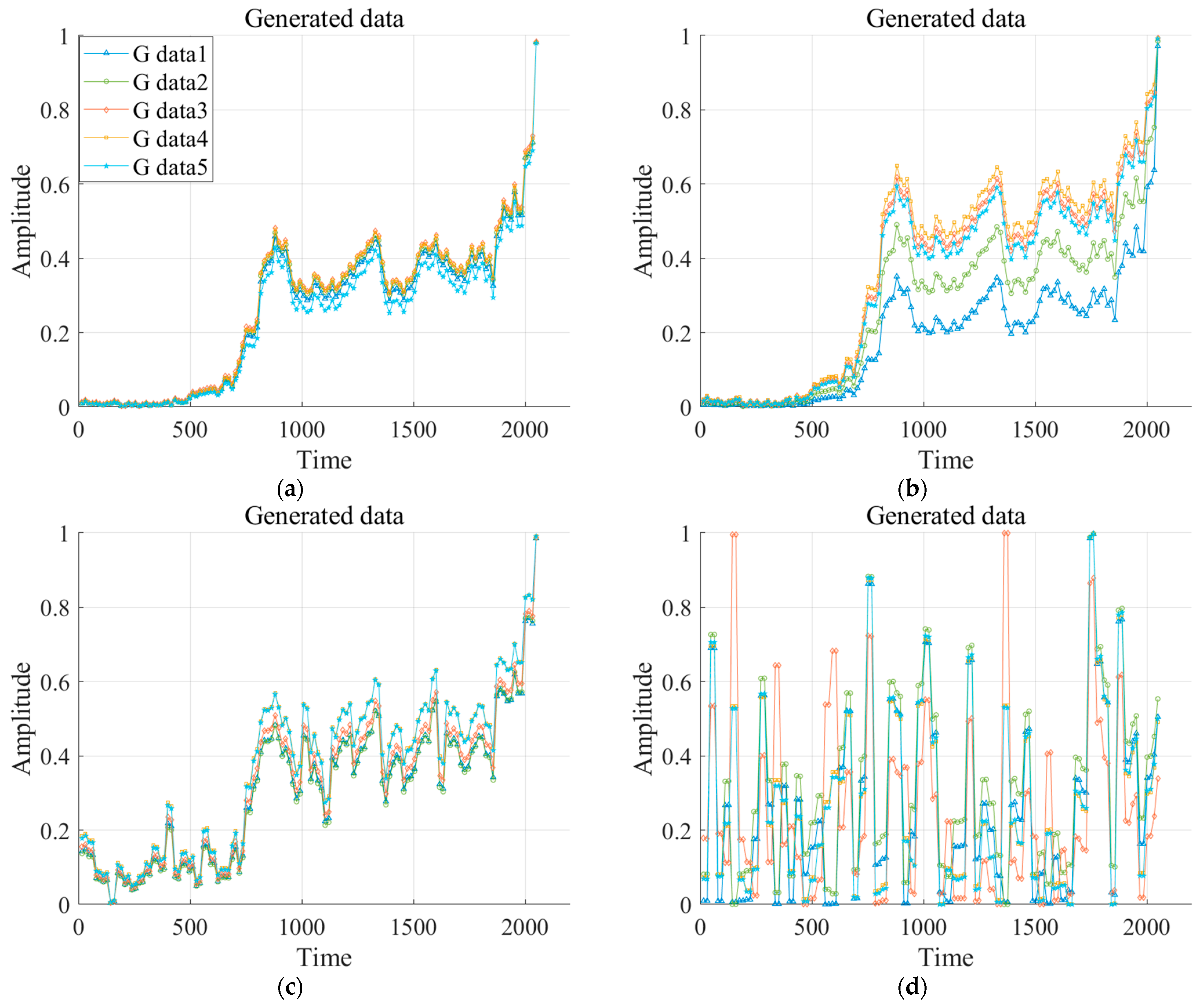
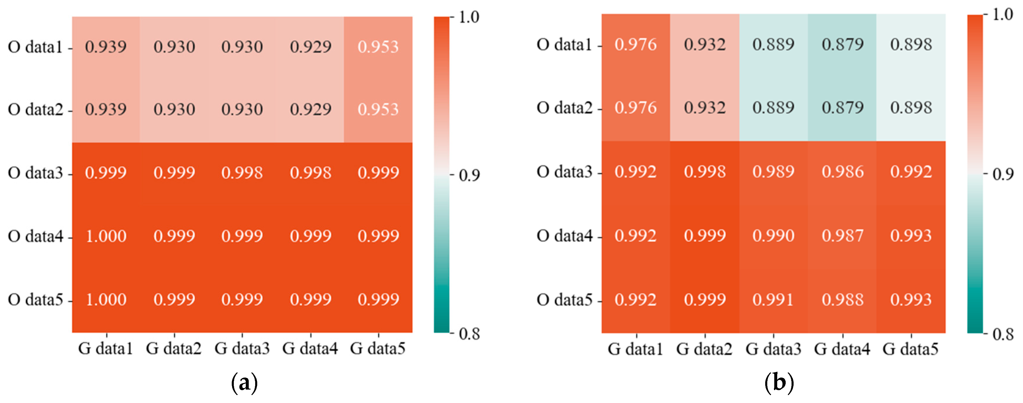
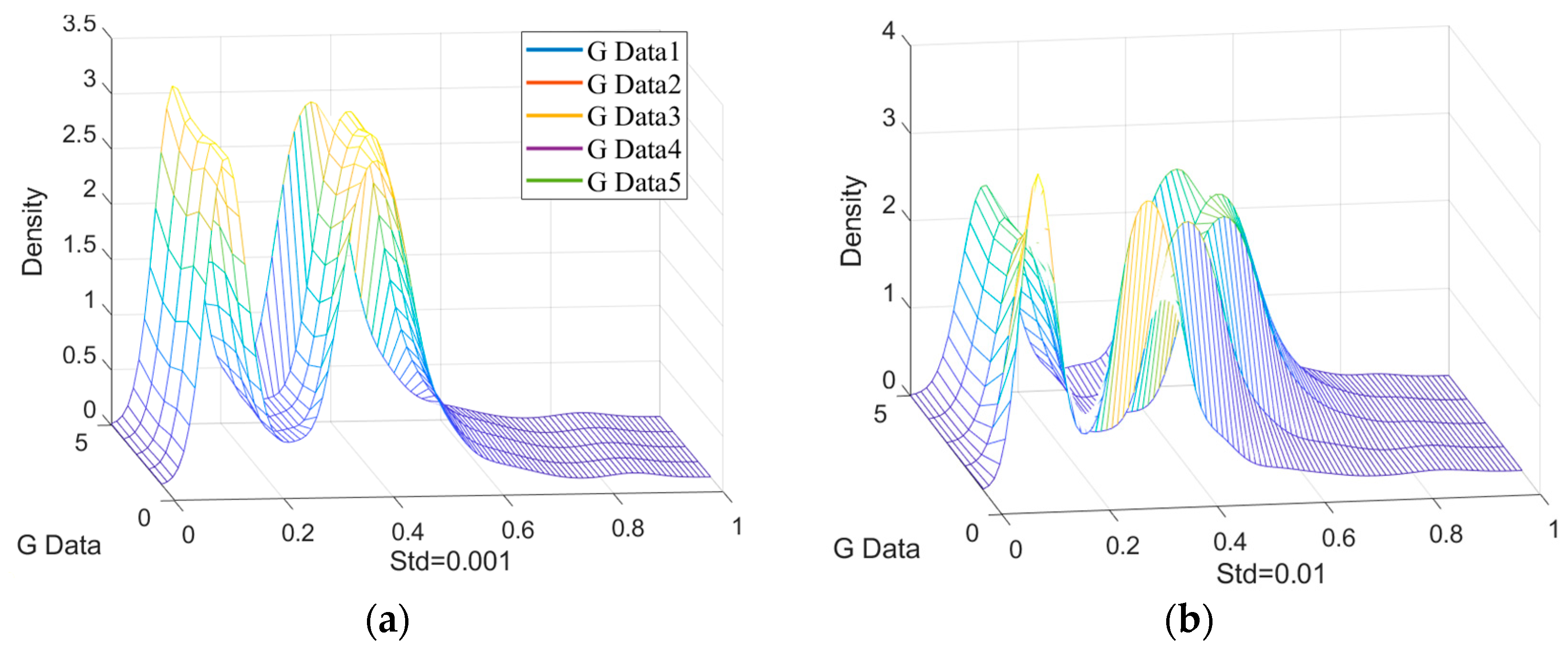
The VAE-GAN model takes these five time-domain features of the training set bearings as input for sample generation; here, the distribution of random noise during the VAE resampling process affects the sampling process, thereby influencing the generation quality of the model and the stability of the learning process. Noise with a large standard deviation increases the distributional diversity of the generated samples, as it increases the range of variation of the hidden variables, which can lead to instability in the training process, while noise with a small standard deviation makes the generated samples more concentrated but lacks a certain degree of diversity. Using Bearing A2 of XJTU-SY dataset as an example, plotting the data generated when the noise standard deviation is set to 1, 0.1, 0.01, and 0.001. As shown in Figure 5c,d, evidently, the generated data are more chaotic when the standard deviation is 1 and 0.1, and the correlation with the original sample is not high. As shown in Figure 5a,b, evidently, the generated data have a more regular shape when the standard deviation is 0.01 and 0.001. To further analyze the generated data, Figure 6 and Figure 7 show the heat map of the correlation coefficient matrix of the feature parameters with standard deviations of 0.01 and 0.001 and the kernel density estimation of the generated data, respectively. In both cases, the generated data exhibit strong correlation with the original data. However, from the three-dimensional kernel density estimation plot, it is observed that the distribution of the generated data becomes highly concentrated when the noise’s standard deviation is set to 0.001, and the generated data lack a certain degree of diversity.

The correlation and diversity should be comprehensively considered. Here, the correlation is defined as the mean correlation (MC) of all the correlation values in the correlation matrix between the generated data and the original data, and the diversity is defined as the mean diversity (MD) of the Euclidean distance between the generated data. The weighted evaluation index was named mean correlation diversity (MCD), where the definition is as follows:

$$MCD=0.7\times Mc+0.3\times Md$$

(14)

Here, the values 0.7 and 0.3 are defined with reference to the ratio of the mean correlation and mean diversity of the original data in the sum of the mean correlation and mean diversity values of the original data.

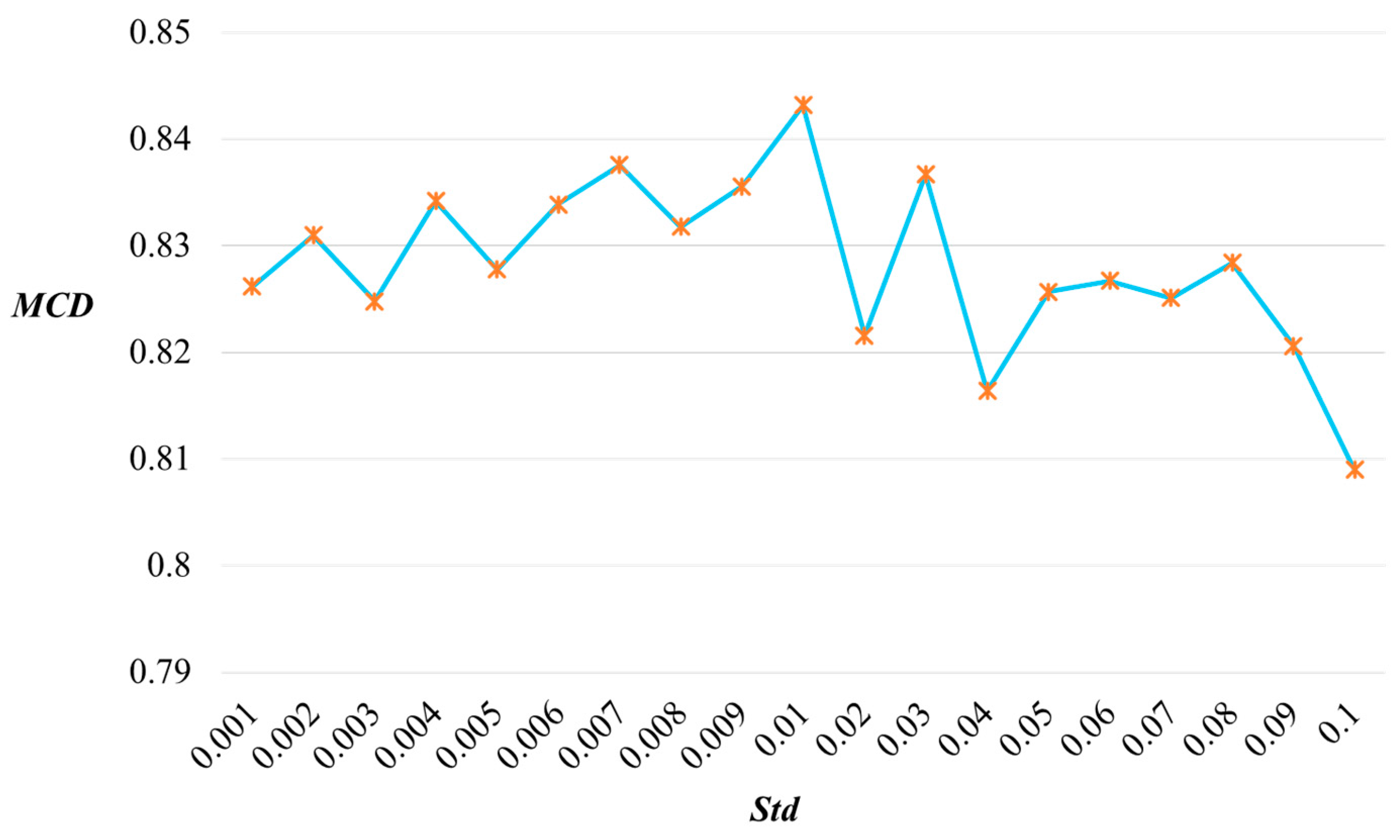
To determine the better standard deviation values, the values of this evaluation indexes are plotted with a standard deviation of 0.001–0.1 in Figure 8, using Bearing A2 as an example:

It is observable that the maximum value of this index is at a standard deviation of 0.01, and MCD values with too large or too small a standard deviation exhibit oscillations around the maximum value. This phenomenon occurs because, in cases where the standard deviation of the data is large, there is high data diversity but relatively lower relevance to the original data. On the other hand, when the standard deviation of the data is small, the data exhibit high relevance, but there may be a lack of diversity in the dataset. Therefore, the standard deviation of noise variable introduced into VAE is set to 0.01.

Since Pearson’s correlation coefficient heat map of the samples generated from the training set Bearing A2 using VAE-GAN with the original samples has been shown in Figure 6, the experiments yielded that the samples generated from the other training sets also exhibit a strong linear correlation with the original samples. Therefore, the heat maps of the correlation coefficients of the other training set bearings are not shown. This indicates that the generated sample maintains the information and structure of the original sample to some extent.

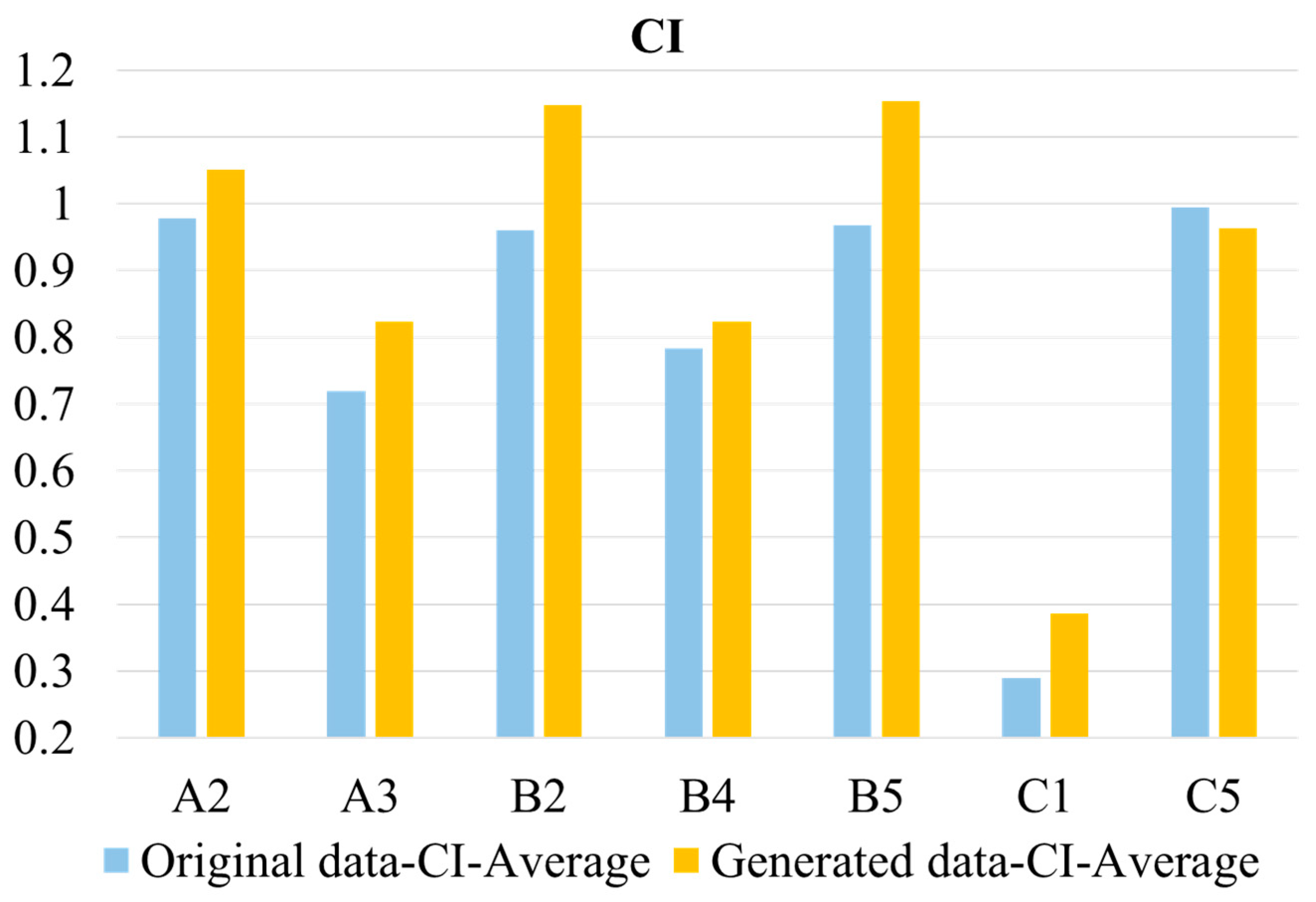
Figure 9 compares the CI values of the generated data with the original data for the training set data, which are shown here after averaging the CI values of the five feature parameters for each bearing. As described in Equation (8) in Section 3.1.2, the CI is calculated as the combination of monotonicity, correlation, and robustness of the data. The values clearly indicate that the CI values of the generated data predominantly surpass those of the original data. This indicates that the generated samples enhance the depiction of the bearing degradation state, potentially improving the model’s performance and the reliability of the RUL prediction outcomes.

4.4. RUL Prediction and Results Discussion on XJTU-SY Bearing Dataset

4.4.1. RUL Prediction Based on Data Augmentation

To demonstrate the superior quality of samples generated by VAE-GAN, the prediction results are compared when the original samples are mixed with different types and numbers of generated samples for the training set. Taking the data in serial number three as an example, the individual datasets are Data1: only the original data (Bearing A2, Bearing A3), Data2: the original data (Bearing A2, Bearing A3) + 100% GAN generated data (G-Bearing A2, G-Bearing A3), Data3: the original data + 200% of the GAN-generated data (2-Bearing A2, 2-Bearing A3), Data4: Original data (Bearing A2, Bearing A3) + 100% VAE-GAN generated data (VG-Bearing A2, VG-Bearing A3).

Table 2. RUL prediction results for mixed data of different types and proportions.

Test Data	Training Data	Metrics
		RMSE	R2-SCORE
Bearing A5	Data1	0.124	0.8069
	Data2	0.1093	0.8499
	Data3	0.0985	0.878
	Data4	0.0984	0.8782

gives some indicators of predicted outcomes:

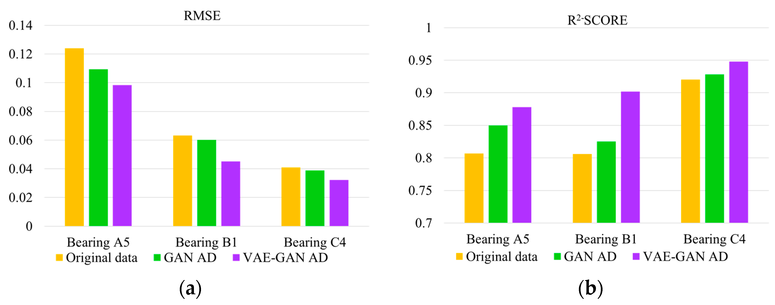
The table illustrates that varying types and quantities of generated data influence the prediction outcomes. The performance of data generated by the GAN is poor. When the training data are the original data and 100% GAN generated data, the prediction result is slightly higher than the original data as the training data, while when the training data are the original data and 200% generated data, the prediction result is close to the original data and 100% VAE-GAN generated data. This shows that VAE-GAN has better performance in sample generation, and the addition of VAE-GAN generated data positively influences the prediction results.

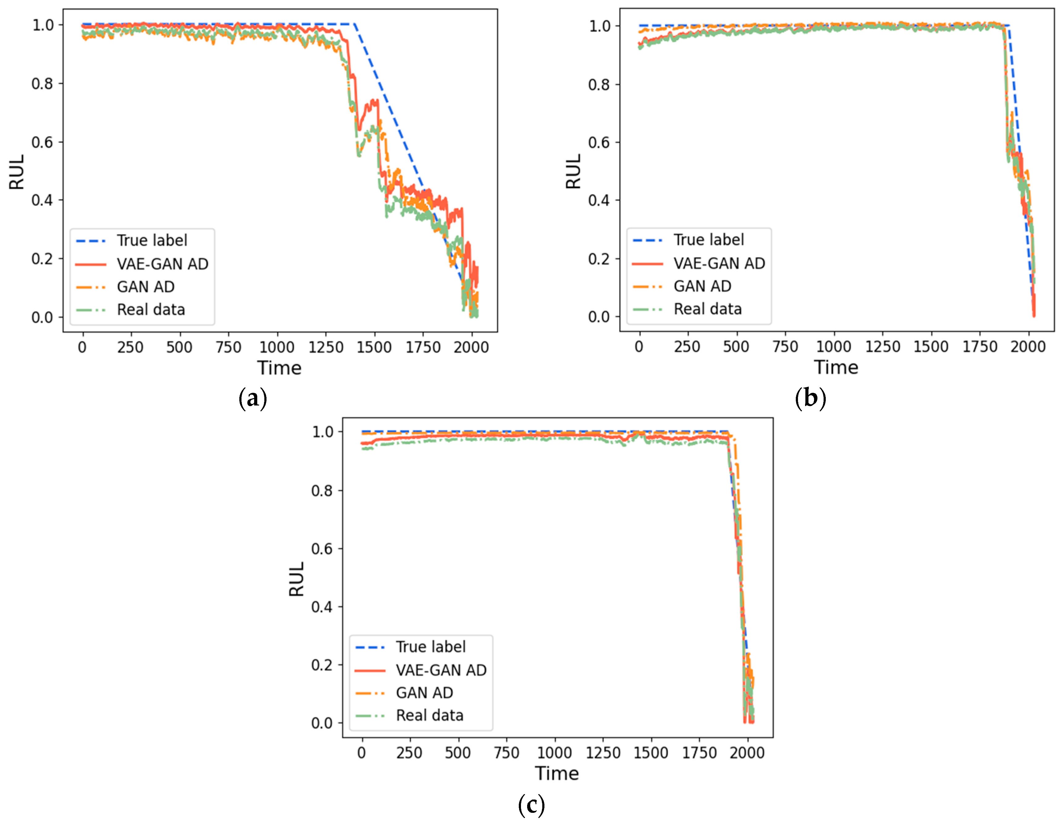
Then, the three kinds of training data used in experiment 1 are the augmented data which is a mixture of VAE-GAN generated data and original data, namely the Data4 above (VAE-GAN Augmented Data, VAE-GAN AD for short), the augmented data which is a mixture of GAN-generated data and original data, namely the Data2 above (GAN Augmented Data, GAN AD for short; here, the number of generation is kept the same as VAE-GAN) and the original data, respectively. The results acquired from the prediction of these three training set data are compared. The results of this experiment are plotted in Figure 10, the evaluation metrics of the prediction results are summarized in

Table 3. RUL prediction evaluation metrics of experiment 1.

Test Set	Training Data	Metrics
		RMSE	R2-SCORE
Bearing A5	VAE-GAN AD	0.0984	0.8782
	GAN AD	0.1093	0.8499
	Original data	0.124	0.8069
Bearing B1	VAE-GAN AD	0.0451	0.9017
	GAN AD	0.0601	0.8251
	Original data	0.0633	0.8061
Bearing C4	VAE-GAN AD	0.0332	0.9478
	GAN AD	0.0389	0.9283
	Original data	0.041	0.9202

. Furthermore, Figure 11 showcases the visualization of the prediction results.

The plots of the prediction results from the three datasets used for RUL show a notable divergence between the predicted and actual RUL in the initial phase of degradation, attributable to the lack of effective degradation information. Predictions are closer to the true RUL when a large amount of degradation information is available during the middle and late phases of degradation. In the case of different training data and the same prediction model, the augmented data generated by VAE-GAN have a smaller RMSE and a higher R²-SCORE, suggesting that the features augmented by VAE-GAN have a more robust regression relationship with the RUL, and the CNN-LSTM prediction model can extract the temporal information more efficiently, leading to enhanced prediction accuracy.

4.4.2. RUL Prediction Based on Data Augmentation and Data Fusion

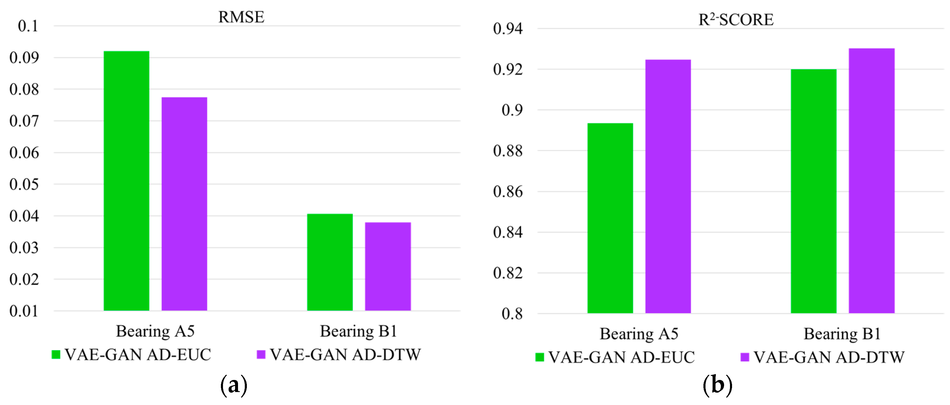
The augmented data and the target data are matched by DTW similarity, and then the weighted fusion data are obtained. The weighted fusion data of each bearing in the training set are trained with the corresponding label input network, and the test data are then applied to the trained network to acquire the RUL prediction results. To demonstrate the advantages of DTW in computing similarity between time series, the two training datasets used in experiment 2 are DTW weighted fusion of VAE-GAN AD (VAE-GAN AD-DTW for short), and the Euclidean distance weighted fusion of VAE-GAN AD (VAE-GAN AD-EUC for short). The results acquired from the prediction of these two training set data are compared. The results of this experiment are plotted in Figure 12, the evaluation metrics of the prediction results are summarized in

Table 4. RUL prediction evaluation metrics of experiment 2.

Test Set	Training Data	Metrics
		RMSE	R2-SCORE
Bearing A5	VAE-GAN AD-DTW	0.0774	0.9247
	VAE-GAN AD-EUC	0.092	0.8935
Bearing B1	VAE-GAN AD-DTW	0.038	0.9302
	VAE-GAN AD-EUC	0.0407	0.9201

. Furthermore, Figure 13 showcases the visualization of the prediction results.

Multi-parameter similarity fusion hinges on the feedback provided by parameters to the degradation process, and the RUL prediction results using the distance metric fluctuate very little around the true value, which not only indicates the effectiveness of the VAE-GAN augmented data, but also demonstrates that the weighted fusion of the training set using the similarity metric captures the correlation of the time series. Compared with Euclidean distance, the similarity measured by DTW algorithm shows superior performance, which manifests as a higher degree of curve fitting. Especially as it approaches the end of its lifespan, the fit becomes increasingly accurate. The prediction results also have smaller RMSE and larger R²-SCORE, indicating that the DTW algorithm outperforms the traditional Euclidean distance in similarity calculation in the analysis of time series.

In order to visualize the advantages of augmented data based on DTW weighted fusion when the above five data types are used as training sets, the visualization of two evaluation metrics of the RUL prediction results is shown in Figure 14. The prediction evaluation metrics of all tested bearings are summarized in

Table 5. RUL prediction evaluation metrics for all tested bearings.

Metrics	Test Set		Training Data
		Original Data	GAN AD	WGAN AD	VAE-GAN AD	VAE-GAN AD-EUC	VAE-GAN AD-DTW
RMSE	Bearing A1	0.1826	0.1379	0.1664	0.1623	0.1574	0.1351
	Bearing A4	0.2062	0.1605	0.1194	0.1507	0.116	0.1042
	Bearing A5	0.124	0.1093	0.1048	0.0984	0.092	0.0774
	Bearing B1	0.0633	0.0601	0.0462	0.0451	0.0407	0.038
	Bearing B3	0.1955	0.1742	0.1597	0.1531	0.1522	0.1489
	Bearing C2	0.124	0.0688	0.2251	0.1017	0.096	0.0865
	Bearing C3	0.0687	0.0566	0.0717	0.055	0.0535	0.0506
	Bearing C4	0.041	0.0389	0.0378	0.0332	0.0281	0.03
	Average	0.1257	0.1008	0.1164	0.0999	0.092	0.0838
R2-SCORE	Bearing A1	0.6255	0.7864	0.6891	0.7043	0.7217	0.7951
	Bearing A4	−13.0796	−7.5248	−3.7245	−6.5208	−3.4587	−2.5951
	Bearing A5	0.8069	0.8499	0.862	0.8782	0.8935	0.9247
	Bearing B1	0.8061	0.8251	0.8968	0.9017	0.9201	0.9302
	Bearing B3	0.5775	0.6648	0.7249	0.7409	0.7439	0.7578
	Bearing C2	−0.5594	0.5197	0.382	−0.0479	0.0658	0.2409
	Bearing C3	0.8277	0.8829	0.8121	0.8896	0.8953	0.9064
	Bearing C4	0.9202	0.9283	0.9323	0.9478	0.9627	0.9575
	Average	0.7607	0.8229	0.8195	0.8438	0.8562	0.8786

.

The outcomes suggest that the proposed method consistently delivers superior results. While Table 5 above shows that some R²-SCORE indicators are negative, and the reason may be that the failure types of test set Bearings A4 and C2 are cage failures or compound failures with cages, but the failure types of training set bearings are both inner and outer ring failures. Generally, it is readily apparent that expanding the data set and introducing similarity analysis into time series can improve the prediction accuracy. Combining DTW similarity weighting with VAE-GAN sample generation method can build fusion data highly similar to the target series to enhance the prediction model, which has important practical application value for time series prediction tasks.

4.5. RUL Prediction and Results Discussion on IMS Dataset and Pantograph Data

4.5.1. Experiment of IMS Dataset

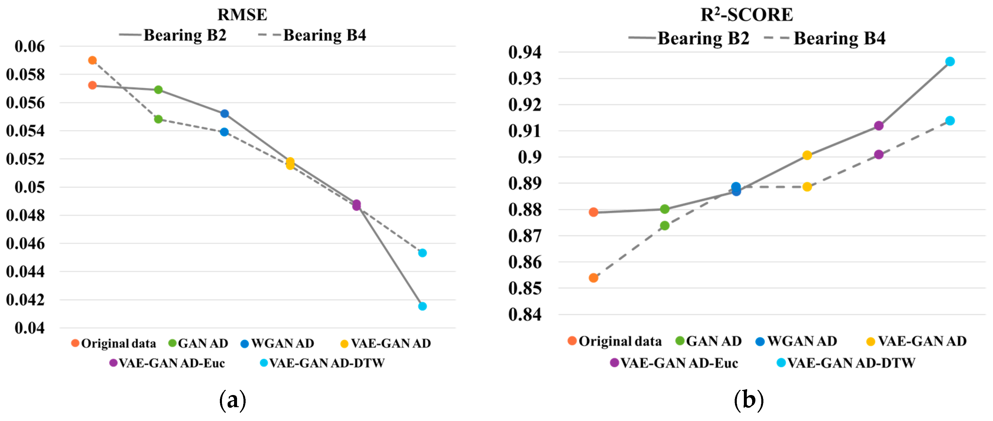
The RUL prediction results on the IMS dataset are plotted in Figure 15, the evaluation metrics of the prediction results are summarized in

Table 6. RUL prediction evaluation metrics on IMS dataset.

Test Set	Training Data	Metrics
		RMSE	R2-SCORE
Bearing B2	VAE-GAN AD-DTW	0.0415	0.9363
	VAE-GAN AD-EUC	0.0488	0.9118
	VAE-GAN AD	0.0518	0.9006
	WGAN AD	0.0552	0.8869
	GAN AD	0.0569	0.8801
	Original data	0.0572	0.8788
Bearing B4	VAE-GAN AD-DTW	0.0453	0.9138
	VAE-GAN AD-EUC	0.0486	0.9008
	VAE-GAN AD	0.0515	0.8886
	WGAN AD	0.0539	0.8778
	GAN AD	0.0548	0.8738
	Original data	0.059	0.8538

. Furthermore, Figure 16 showcases the visualization of the prediction results.

According to the above prediction result graph and evaluation metrics, data augmentation and similarity fusion can also improve the prediction accuracy of bearings well on the IMS dataset.

4.5.2. Experiment of Pantograph Data

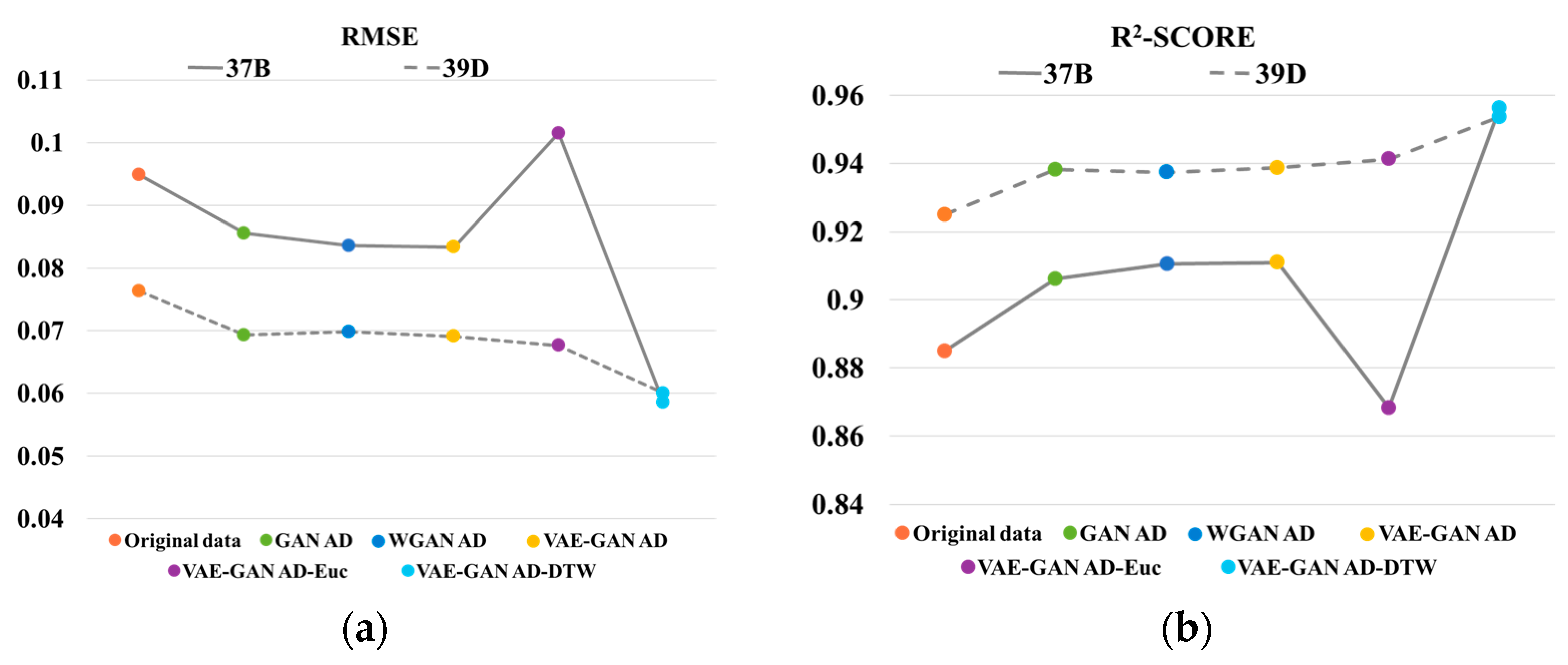
The RUL prediction results on the pantograph data are plotted in Figure 17, the evaluation metrics of the prediction results are summarized in

Table 7. RUL prediction evaluation metrics on pantograph data.

Test Set	Training Data	Metrics
		RMSE	R2-SCORE
37B	VAE-GAN AD-DTW	0.0585	0.9562
	VAE-GAN AD-EUC	0.1015	0.8682
	VAE-GAN AD	0.0834	0.911
	WGAN AD	0.0836	0.9106
	GAN AD	0.0856	0.9062
	Original data	0.0949	0.8849
39D	VAE-GAN AD-DTW	0.06	0.9537
	VAE-GAN AD-EUC	0.0676	0.9413
	VAE-GAN AD	0.0691	0.9387
	WGAN AD	0.0698	0.9374
	GAN AD	0.0693	0.9382
	Original data	0.0764	0.925

. Furthermore, Figure 18 showcases the visualization of the prediction results.

From the above prediction results, it can be seen that the DTW weighted fused augmented data have the best curve fit when used as training data. Combining DTW similarity with sample generation can effectively improve the model fitting ability and prediction accuracy, which has important practical applications for the task of time series prediction.

5. Conclusions

We unveiled an RUL prediction methodology that accomplished data augmentation and fusion for feature parameters. Firstly, sample generation of degraded features was executed by VAE-GAN. Then, RUL prediction was performed on augmented data based on DTW similarity fusion. Experiments on the XJTU-SY rolling element bearing accelerated life test dataset, IMS dataset, and pantograph data were performed to demonstrate the efficacy of generating samples and implementing similarity fusion, which showed good performance in RUL prediction.

(1)

When insufficient raw data lead to imprecise RUL prediction results, data augmentation using a generative model could optimize the prediction results, making the model prediction results with mixed data more accurate than the model prediction of life using only original data.

(2)

In RUL prediction, a DTW-based nonlinear programming algorithm was introduced for the distance measure of similarity, which outperformed the traditional Euclidean distance in the similarity analysis of time series. Multi-parameter fusion was performed on the augmented data, and the constructed feature parameters contained sufficient degradation information, which improved the accuracy of the prediction models.

Future research will optimize the prediction model, improve the model’s ability to capture complex time series patterns, as well as enhance the explanatory and interpretable nature of the prediction model.

References

1. He, Z.; Shao, H.; Lin, J.; Cheng, J.; Yu, Y. Transfer fault diagnosis of bearing installed in different machines using enhanced deep auto-encoder. Measurement 2020, 152, 107393. [Google Scholar]
2. Shao, H.; Xia, M.; Han, G.; Zhang, Y.; Wan, J. Intelligent fault diagnosis of rotor-bearing system under varying working conditions with modified transfer convolutional neural network and thermal images. IEEE Trans. Ind. Inform. 2020, 17, 3488–3496. [Google Scholar] [CrossRef]
3. Sikorska, J.Z.; Hodkiewicz, M.; Ma, L. Prognostic modelling options for remaining useful life estimation by industry. Mech. Syst. Signal Process. 2011, 25, 1803–1836. [Google Scholar] [CrossRef]
4. Wang, B.; Li, H.; Xu, B. Motor bearing forecast feature extracting and degradation status identification based on multi-scale morphological decomposition spectral entropy. J. Vib. Shock 2013, 32, 124–128. [Google Scholar]
5. Li, H.; Yu, H.; Tian, Z.; Li, B. Degradation trend prediction of rolling bearings based on two-element multiscale entropy. China Mech. Eng. 2017, 28, 2420–2425, 2433. [Google Scholar]
6. Gebraeel, N.; Lawley, M.; Liu, R.; Parmeshwaran, V. Residual life predictions from vibration-based degradation signals: A neural network approach. IEEE Trans. Ind. Electron. 2004, 51, 694–700. [Google Scholar] [CrossRef]
7. Wang, Y.; Peng, Y.; Zi, Y.; Jin, X.; Tsui, K.-L. A two-stage data-driven-based prognostic approach for bearing degradation problem. IEEE Trans. Ind. Inform. 2016, 12, 924–932. [Google Scholar] [CrossRef]
8. Xia, Z.; Xia, S.; Wan, L.; Cai, S. Spectral regression based fault feature extraction for bearing accelerometer sensor signals. Sensors 2012, 12, 13694–13719. [Google Scholar] [CrossRef]
9. Fu, B.; Yuan, W.; Cui, X.; Yu, T.; Zhao, X.; Li, C. Correlation analysis and augmentation of samples for a bidirectional gate recurrent unit network for the remaining useful life prediction of bearings. IEEE Sens. J. 2020, 21, 7989–8001. [Google Scholar] [CrossRef]
10. Ping, G.; Chen, J.; Pan, T.; Pan, J. Degradation feature extraction using multi-source monitoring data via logarithmic normal distribution based variational auto-encoder. Comput. Ind. 2019, 109, 72–82. [Google Scholar] [CrossRef]
11. Que, Z.; Xiong, Y.; Xu, Z. A semi-supervised approach for steam turbine health prognostics based on GAN and PF. In Proceedings of the 2019 IEEE International Conference on Industrial Engineering and Engineering Management (IEEM), Macao, China, 15–18 December 2019; IEEE: Piscataway, NJ, USA, 2019; pp. 1476–1480. [Google Scholar]
12. Liu, S.; Chen, J.; Qu, C.; Hou, R.; Lv, H.; Pan, T. LOSGAN: Latent optimized stable GAN for intelligent fault diagnosis with limited data in rotating machinery. Meas. Sci. Technol. 2021, 32, 045101. [Google Scholar] [CrossRef]
13. Lu, H.; Barzegar, V.; Nemani, V.P.; Hu, C.; Laflamme, S.; Zimmerman, A.T. Joint training of a predictor network and a generative adversarial network for time series forecasting: A case study of bearing prognostics. Expert Syst. Appl. 2022, 203, 117415. [Google Scholar] [CrossRef]
14. Lei, L.; Li, X.; Wen, J.; Miao, J. Data Amplification for Bearing Remaining Useful Life Prediction Based on Generative Adversarial Network. Wirel. Commun. Mob. Comput. 2022, 2022, 4628462. [Google Scholar] [CrossRef]
15. Frid-Adar, M.; Diamant, I.; Klang, E.; Amitai, M.; Goldberger, J.; Greenspan, H. GAN-based synthetic medical image augmentation for increased CNN performance in liver lesion classification. Neurocomputing 2018, 321, 321–331. [Google Scholar] [CrossRef]
16. Ma, X.; Jin, R.; Sohn, K.A.; Paik, J.-Y.; Chung, T.-S. An adaptive control algorithm for stable training of generative adversarial networks. IEEE Access 2019, 7, 184103–184114. [Google Scholar] [CrossRef]
17. Larsen AB, L.; Sønderby, S.K.; Larochelle, H.; Winther, O. Autoencoding beyond pixels using a learned similarity metric. In Proceedings of the International Conference on Machine Learning, New York, NY, USA, 20–22 June 2016; pp. 1558–1566. [Google Scholar]
18. Wang, X.; Jiang, H.; Liu, Y.; Yang, Q. Data-augmented patch variational autoencoding generative adversarial networks for rolling bearing fault diagnosis. Meas. Sci. Technol. 2023, 34, 055102. [Google Scholar] [CrossRef]
19. Nie, L.; Zhang, L.; Xu, S.; Cai, W.; Yang, H. Remaining useful life prediction of rolling bearings based on similarity feature fusion and CNN. Noise Vib. Control 2023, 43, 115. [Google Scholar]
20. Hou, M.; Pi, D.; Li, B. Similarity-based deep learning approach for remaining useful life prediction. Measurement 2020, 159, 107788. [Google Scholar] [CrossRef]
21. Nguyen, T.S. Hybridising neural network and pattern matching under dynamic time warping for time series prediction. Int. J. Bus. Intell. Data Min. 2020, 17, 54–75. [Google Scholar] [CrossRef]
22. Li, H.; Guo, C. A review of research on feature representation and similarity metrics in time series data mining. Comput. Appl. Res. 2013, 30, 1285–1291. [Google Scholar]
23. Song, L.; Jin, Y.; Lin, T.; Zhao, S.; Wei, Z.; Wang, H. Remaining Useful Life Prediction Method Based on the Spatiotemporal Graph and GCN Nested Parallel Route Model. IEEE Trans. Instrum. Meas. 2024, 73, 3511912. [Google Scholar] [CrossRef]
24. Lei, Y.; Li, N.; Gontarz, S.; Lin, J.; Radkowski, S.; Dybala, J. A Model-Based Method for Remaining Useful Life Prediction of Machinery. IEEE Trans. Reliab. 2016, 65, 1314–1326. [Google Scholar] [CrossRef]
25. Zhang, B.; Zhang, L.; Xu, J. Degradation feature selection for remaining useful life prediction of rolling element bearings. Qual. Reliab. Eng. Int. 2016, 32, 547–554. [Google Scholar] [CrossRef]
26. Lin, T.; Song, L.; Cui, L.; Wang, H. Advancing RUL prediction in mechanical systems: A hybrid deep learning approach utilizing non-full lifecycle data. Adv. Eng. Inform. 2024, 61, 102524. [Google Scholar] [CrossRef]
27. Lei, Y.; Han, T.; Wang, B.; Li, N.; Yan, T.; Yang, J. XJTU-SY Rolling Element Bearing Accelerated Life Test Datasets: A Tutorial. J. Mech. Eng. 2019, 55, 1–6. [Google Scholar]
Figure 1. The framework of proposed method.
Vibration 07 00029 g001
Figure 2. Structure of VAE.
Vibration 07 00029 g002
Figure 3. Structure of GAN.
Vibration 07 00029 g003
Figure 4. Test bed. (a) XJTU-SY bearing dataset; (b) IMS dataset; (c) Slide plates of pantograph.
Vibration 07 00029 g004
Figure 5. Generated data by VAE-GAN with noise standard deviation of different value. (a) value = 0.001; (b) value = 0.01; (c) value = 0.1; (d) value = 1.
Vibration 07 00029 g005
Figure 6. The correlation coefficients matrix heat map of feature parameter with different noise standard deviation. (a) value = 0.001; (b) value = 0.01.
Vibration 07 00029 g006
Figure 7. The kernel density map of generated data with different noise standard deviation. (a) value = 0.001; (b) value = 0.01.
Vibration 07 00029 g007
Figure 8. MCD values at different standard deviations.
Vibration 07 00029 g008
Figure 9. CI values of training set.
Vibration 07 00029 g009
Figure 10. RUL prediction results of experiment 1. (a) Bearing A5; (b) Bearing B1; (c) Bearing C4.
Vibration 07 00029 g010
Figure 11. Visualization of RUL prediction of experiment 1. (a) RMSE; (b) R2-SCORE.
Vibration 07 00029 g011
Figure 12. RUL prediction results of experiment 2. (a) Bearing A5; (b) Bearing B1.
Vibration 07 00029 g012
Figure 13. Visualization of RUL prediction of experiment 2. (a) RMSE; (b) R2-SCORE.
Vibration 07 00029 g013
Figure 14. Visualization of RUL prediction under different training data. (a) RMSE; (b) R2-SCORE.
Vibration 07 00029 g014
Figure 15. RUL prediction results on IMS dataset. (a)Bearing B2; (b)Bearing B4.
Vibration 07 00029 g015
Figure 16. Visualization of RUL prediction results on IMS dataset. (a) RMSE; (b) R2-SCORE.
Vibration 07 00029 g016
Figure 17. RUL prediction results on pantograph data. (a) 37B; (b) 39D.
Vibration 07 00029 g017
Figure 18. Visualization of RUL prediction results on pantograph data. (a) RMSE; (b) R2-SCORE.
Vibration 07 00029 g018