A Deep Transfer Learning Model for the Fault Diagnosis of Double Roller Bearing Using Scattergram Filter Bank 1

Abstract

In this study, a deep transfer learning model was developed using ResNet-101 architecture to diagnose double roller bearing defects. Vibration data were collected for three different load scenarios, including conditions without load, and for five different rotational speeds, ranging from 500 to 2500 RPM. Significantly, the speed condition of 2500 RPM has not previously been investigated, therefore offering a potential avenue for future investigations. This study offers a thorough examination of bearing conditions using multidirectional vibration data collected from accelerometers positioned in both vertical and horizontal orientations. In addition to transfer learning using ResNet-101, four additional models (VGG-16, VGG19, ResNet-18, and ResNet-50) were trained. Transfer learning using ResNet-101 consistently achieved the highest accuracy in all scenarios, with accuracy rates ranging from 90.78% to 99%. Scattergram Filter Bank 1 was used as the image input for training as a preprocessing method to enhance feature extraction. Research has effectively applied transfer learning to improve fault diagnosis accuracy, especially in limited data scenarios. This shows the capability of the method to differentiate between normal and faulty bearing conditions using signal-to-image transformation, emphasizing the potential of transfer learning to augment diagnostic performance in scenarios with limited training data.

1. Introduction

Bearing failures in rotating machinery lead to unplanned downtime, safety risks, and millions in lost revenue annually. Traditional diagnostic methods often struggle to detect early-stage faults in harsh operating environments, limiting the effectiveness of predictive maintenance. The significance of bearings is underscored by the severe implications of their failure, highlighting the need for effective fault diagnosis. Traditional methods, which typically rely on diagnostic approaches, primarily based on manual inspections and elementary statistical methods, are increasingly being replaced by more advanced techniques, especially in the realm of machine learning. A significant stride in this field is the emergence of deep learning methodologies, as highlighted by Zhao et al. [1]. The role of bearing fault detection and diagnosis as key aspects of predictive maintenance in rotating machinery is well established, with vibration signals serving as the main diagnostic medium due to their direct correlation with bearing health, as reported by Ma et al. [2].

In addition to the development of fault diagnosis methods, the establishment and collection of benchmark datasets is essential. Notable fault diagnosis datasets include those from Case Western Reserve University [3], the IEEE PHM 2012 Data Challenge [4], the University of Cincinnati [5], the University of Ottawa [6], and Xi’an Jiao Tong University [7]. These datasets, which are publicly available and considered state-of-the-art, contain a wide range of rolling bearing operation data and are described in detail in their corresponding references. For fault detection problems, a representative signal segment is often subjectively selected from the data collected for analysis, which can affect the detection performance of the methods applied. Moreover, these datasets might require preprocessing to test the effectiveness of proposed fault-type recognition methods, such as dividing the data into training and testing sets for machine learning-based methods. While these datasets are instrumental, the necessity remains for sharing and developing diverse datasets for rolling bearing fault diagnosis tasks, echoing the significance of datasets like ImageNet [8] in the computer vision community. Deep learning-based methods for rolling bearing fault type recognition can automate feature extraction, reduction, and classification, but they often require significant manual effort in designing network architectures and adjusting parameters, which can be time-consuming and resource-intensive. Additionally, these methods typically lack interpretability and require a large number of samples for training, a challenging requirement in practical engineering applications where fault samples are scarce. Therefore, there is a compelling need for new fault-type recognition methods that are less reliant on extensive manual effort and can effectively handle limited training data while offering interpretable models for fault identification [9]. The existing methods, despite their advancements, still necessitate considerable prior knowledge and expert experience, highlighting the need for more intelligent and flexible approaches that can adapt to a broad range of applications without heavy reliance on domain-specific expertise.

The studies by Singh and Moore (2021) [10] and Singh and Moore (2020) [11] on nonlinear system identification characteristic nonlinear system identification (CNSI) for local attachments provided valuable information for bearing fault diagnosis. The 2021 research demonstrated the applicability of the CNSI method for multiple attachments and interactions with higher modes, which can be crucial for accurately diagnosing bearing faults that manifest through complex dynamic behaviors. Similarly, the 2020 study’s focus on clearance nonlinearities extended the utility of CNSI for identifying the dynamics of bearing systems with nonlinear characteristics, such as those found in faulty bearings. These methodologies could improve bearing fault diagnosis by offering a more nuanced understanding of the dynamic responses of bearings under various fault conditions [12]. In bearing fault diagnostics, developing more accurate and predictive maintenance strategies is crucial.

The performance of fault-type recognition methods often presupposes that training and test samples are independently and identically distributed. However, variations in working conditions, such as changes in characteristic frequencies and amplitudes through different rotational speeds, can introduce significant differences between training and testing data, leading to domain adaptation challenges. Transfer learning (TL) has emerged as a promising approach to address these challenges by leveraging knowledge from related domains to improve learning performance in target scenarios [4,12,13]. Despite the success of TL-based methods, further research is needed to enhance their domain adaptability and recognition accuracy, especially under variable operating conditions. Furthermore, a reliance on large volumes of labeled data poses significant challenges, particularly in obtaining fault samples, which are rare and labour-intensive to label. Few-shot learning (FSL) offers a viable solution for accurate failure attribution under conditions of limited data availability, with data augmentation, data/model transfer, and metalearning being key strategies in FSL methods [9].

Recent advancements have identified the use of multidirectional vibration data as more effective than traditional single-directional vibration signals for bearing fault diagnostics. This method enhances the accuracy and reliability of bearing failure detections, as noted by Zhang & Gu [14]. However, a primary challenge in this area is the inherent heterogeneity of datasets, which can differ in aspects such as experimental conditions, fault severity, fault types, and setup configurations, and setup configurations, a point highlighted by Chen et al. [15]. Conventional diagnostic models often fail due to their assumption of uniform feature distribution in training and testing data, an assumption rarely met in practical scenarios. This discrepancy often diminishes the effectiveness of traditional machine learning models in various applications, as Bhuiyan and Uddin [16] have observed.

The shift towards multidirectional vibration data in bearing failure diagnostics marks a substantial improvement over the analysis of single-direction signals. This approach, as reiterated by Zhang and Gu [14], significantly refines precision and reliability in the identification of bearing malfunctions. The study by Han, Xie, and Pei innovatively addresses the challenges of fault diagnosis in wind turbines through a semi-supervised adversarial learning approach, leveraging both annotated and unannotated data to enhance diagnostic accuracy amidst the scarcity of labeled data (Han, Xie, & Pei, 2023 [17]. By integrating adversarial learning with metric learning techniques, the research not only significantly contributes to the wind energy sector by improving the reliability of fault diagnosis methods, but also presents a methodology adaptable across various domains, highlighting its broader implications for the renewable energy sector and beyond. This advancement supports the operational stability of wind turbines, furthering sustainable energy transition efforts.

Recent research by Kaya, Kuncan, and Ertunç [18] demonstrated the effectiveness of using time–frequency images obtained from Continuous Wavelet Transform (CWT) combined with deep transfer learning DTL methods for the automatic diagnosis of bearing fault sizes. Their study utilized various pre-trained networks, such as AlexNet, GoogleNet, ResNet, VGG16, and VGG19, achieving high classification accuracy rates between 96.67% and 100%, and showcasing the potential of DTL in bearing diagnostics [18].

The importance of deep transfer learning (DTL) in fault diagnosis is further supported by a systematic review conducted by Singh and Singh [19], which underscored the efficiency of DTL in processing and analyzing vibration signal data for identifying anomalies in roller bearings. This review highlighted the transition towards more sophisticated AI-based diagnostic techniques, emphasizing the advantages of leveraging pre-trained models through DTL [19].

In addition, the work of Zhang and Zhou [20] on the integration of machine learning techniques into condition monitoring systems echoed the importance of adopting advanced algorithms for fault diagnosis. Their review encapsulated the growing trend of using deep learning models, including those enabled by deep transfer learning (DTL), to effectively predict equipment failures [20].

The effectiveness of DTL in bearing fault diagnosis, especially in scenarios characterized by limited data availability, is also evident in research by Li and Zhang [21],and Wang and Zhao [22]. These studies highlighted how DTL models can be adapted from large datasets to specific diagnostic tasks, thus improving the performance of the model in detecting bearing failures [23,24].

Lastly, research by [25] into the application of deep learning for fault diagnosis indicated the method’s potential to significantly improve diagnostic processes. This study emphasized the utility of pre-trained models in DTL approaches to circumvent the limitations inherent in traditional diagnostic methods [25].

Incorporating vibration data from multiple directions in fault diagnosis provides several advantages:

• By analyzing vibrations from different angles, it is possible to detect subtle fault characteristics that might be missed in a single-direction signa.
• Multidirectional vibration data provide additional information on the location of the fault, allowing for more accurate identification.
• Noise can significantly affect the accuracy of fault diagnosis. Using vibration data from multiple directions can help suppress noise, thus isolating fault-related signals more effectively.

Challenges persist due to the intrinsic heterogeneity of datasets, varying in experimental settings, fault severity, and types.

Traditional models often struggle in these scenarios, primarily because they are built on the assumption of consistent data distribution across training and testing phases—a rarity in real-world settings [16,26]. In order to address these issues, the current focus on deep transfer learning in industrial machinery fault diagnosis, particularly for bearings, represents a significant advancement. This approach uses knowledge from one domain to enhance learning in another and has shown notable effectiveness in scenarios characterized by limited labeled data, diverse operational conditions, and feature distribution discrepancies [27,28]. Various deep transfer learning techniques, including fine-tune-based, statistic-based, adversarial-based, and few-shot-based approaches, have demonstrated promising results in developing robust diagnostic models [28,29,30]. Recent advances in the field of bearing fault diagnosis have heavily leaned on the capabilities of deep learning (DL) technologies, particularly convolutional neural networks (CNNs). Studies have utilized architectures like VGG16, VGG19, and ResNet to significantly improve fault classification accuracy by exploiting their deep feature extraction capabilities from vibration signal data. For instance, the use of CNNs for feature extraction has been pivotal in capturing subtle patterns in vibration signals that are often missed by traditional methods [31,32]. However, despite these advancements, the application of transfer learning to adapt these deep networks, pre-trained on generic datasets to specific diagnostic tasks in bearing fault, remains underexplored. This points towards a significant research gap where the potential of transfer learning could be harnessed to reduce dependency on large, labeled datasets specific to bearing faults. Another critical gap lies in the real-time application of these advanced models. The computational demands of architectures like ResNet and VGG19 often limit their deployment in real-time scenarios where quick fault detection is crucial to prevent machinery downtime [29,30]. Furthermore, most current research focuses on offline analysis, with less attention given to the challenges of integrating these models within live operational monitoring systems. There is a pressing need for developing lightweight models or optimizing existing architectures to operate efficiently in real-time conditions without compromising diagnostic accuracy.

The necessity for new work in this area stems from the evolving complexity of machinery and operational conditions under which these bearing systems operate. As industrial machinery becomes more sophisticated, the vibration patterns associated with faults become more complex, requiring more nuanced detection capabilities [29]. Additionally, the integration of physical domain knowledge with DL models presents an underexplored area of research that could potentially lead to more robust diagnostic systems that are adaptable to varying operational contexts and can handle noisy data more effectively [33].

Our research builds on these findings, employing the TL_ResNet-101 model in transfer learning to enhance the detection of early-stage bearing faults, extending the work of Zhao et al. [34]. Furthermore, we address the challenge of data heterogeneity using multidirectional vibration data, following the recommendation of Bhuiyan and Uddin [16] for adaptable models under varying operational conditions.

The availability of open-source bearing failure datasets, which include both experimentally induced faults and run-to-failure data, has been instrumental in advancing and validating these models in controlled environments. However, the scarcity of accurately labeled target fault data continues to be a significant barrier, making traditional training methods impractical for many industrial [35,36,37]. Transfer learning offers a solution to this by applying knowledge from one domain to improve learning in another, thus addressing the issue of insufficient labeled data and enhancing the flexibility and applicability of diagnostic models [38].

Despite these advances, the application of advanced, complex deep learning structures like ResNet-101 in the diagnosis of spherical bearings remains underexplored. The ResNet-101 model, known for its exceptional image recognition capabilities, can significantly improve mechanical fault diagnosis when adapted through transfer [39,40,41]. This study aims to merge a multidirectional vibration data analysis, which offers a comprehensive insight into bearing states, with advanced machine learning algorithms [42].

The primary contributions of our study are as follows:

• Introducing the innovative application of ResNet-101 architecture, renowned for its efficacy in image recognition, spherical bearing fault diagnosis, and employing signal-to-image conversion techniques.
• Utilizing multidirectional vibration data to enhance the detection of nuanced fault characteristics and provide additional information on fault location, thereby improving the isolation of the fault and the suppression of noise, thus isolating fault-related signals more effectively.
• Enhancing accuracy in the diagnosis of early-stage faults, even under limited data availability, and enhancing adaptability to diverse operating conditions and bearing configurations.
• Merging transfer learning with the ResNet-101 framework to tackle the complexities of signal processing and data uniqueness in different operational scenarios, promising a substantial improvement in the precision and efficiency of defect identification in spherical bearings, especially double row spherical roller bearings.

2. Materials and Methods

2.1. Experimental Work

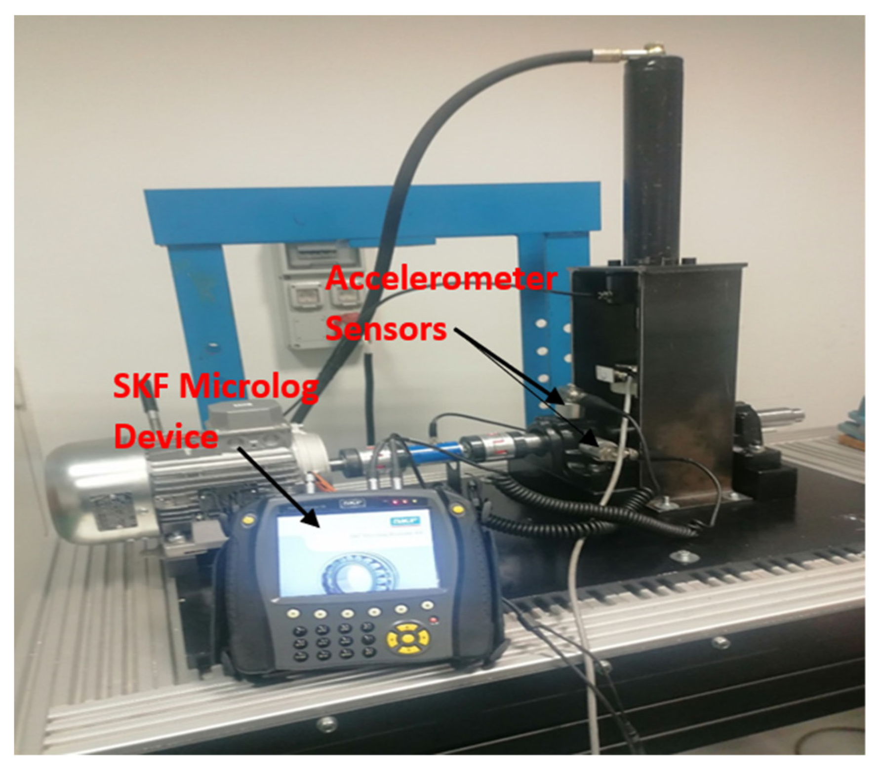
The experimental setup is illustrated in Figure 1. The shaft was driven by a variable-speed motor controlled by an AC driver. Two bearing housings were used to support the shaft. Bearing housing 2 on the right side was healthy. On the contrary, bearing housing 1 on the left side was replaced with different defective bearings. The loading system consisted of a hydraulic pump attached to the frame, which applied pressure to the load sensor on the bearing frame. These bearings included a healthy bearing (HB), a bearing with a defect on a spherical roller (RF), a bearing with an outer race defect (ORF), and a bearing with an inner race defect (IRF). Two accelerometers were installed on the bearing housing in two vertical and horizontal directions to collect vibration signals in the vertical and horizontal directions. A tachometer was used to measure the shaft rotation speed to validate the proposed method. The signals were collected with an SKF Microlog CMX80 instrument (Made by SKF, SKF is a Swedish company headquartered in Gothenburg, Sweden.) and sampled using SKF Report and analysis software.

2.2. Spherical Rolling Bearing SKF 22209 EK

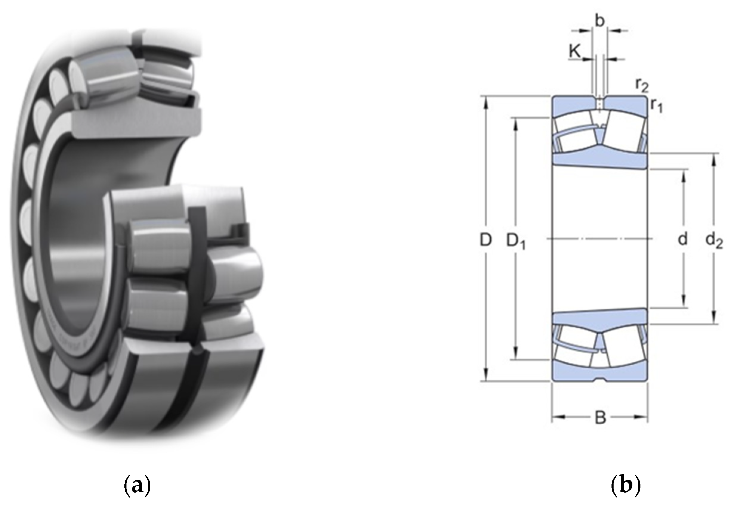
SKF 22209EK is a high-performance spherical roller bearing from the Explorer series, designed for high-speed applications with high radial loads, axial loads, and tilting moments. It is suitable for the mining, construction, agriculture, and transportation industries. The bearing had a tapered bore with a 1:12 taper for easy installation and removal. It had two rows of symmetrical rollers with a common spherical raceway in the outer ring, compensating for misalignments and shaft deflections. It can operate at a maximum speed of 8500 RPM and a maximum operating temperature of 200 °C. Its high radial internal clearance reduced the risk of thermal expansion damage. The inner raceway was mounted on the shaft, whereas the outer raceway was in the housing. The bearing had 34 rollers arranged in two rows, with a common spherical raceway in the outer ring. This model has not previously been used for bearing fault diagnosis, providing an opportunity to explore its characteristics and suitability for fault detection, and enriching current research in this area. The dimensions of the SKF 22209EK spherical roller bearing are illustrated in Figure 2b and in

Table 1. SKF 22209EK spherical roller bearing dimensions [43].

Bore diameter d	45 mm
Outside diameter D	85 mm
Width B	23 mm
Outside diameter D	85 mm
Shoulder diameter of inner ring d2	≈54.4 mm
Shoulder/recess diameter of outer ring D1	≈74.4 mm
Width of lubrication groove b	5.5 mm
Diameter of lubrication hole K	3 mm
Chamfer dimension r1,2	min. 1.1 mm

below:

The SKF22209 EK bearing was chosen specifically for its design flexibility, allowing for the disassembly and reassembly of parts without compromising its operational integrity. This design facilitates the controlled introduction of defects such as wear, pits, or cracks into the roller, outer race, and inner race for experimental purposes.

Concerns are addressed as follows:

• Disassembly and reassembly process: The bearing design allows for the removal and replacement of rollers, especially by extracting two rollers along the same line. This method also applies to other defective parts. The process was conducted with precision tools and under strict guidelines to ensure accurate positioning and orientation of components upon reassembly.
• Quality Assurance of Reassembly: After introducing the defects and reassembling the bearing, several quality checks were performed:
  • Dimensional Inspection: We Ensured all parts were fitted correctly and there were no unintended gaps or misalignments.
  • Rotational Testing: The bearing was subjected to low-speed rotation tests to detect any anomalies in smoothness or noise that could indicate improper assembly.

Vibration analysis: Before and after introducing defects, a vibration analysis was conducted. The comparison helped in confirming that any new vibration signatures were solely due to the introduced defects and not from assembly issues.

2.3. Artificial Defects Using Electrical Discharge Machining (EDM)

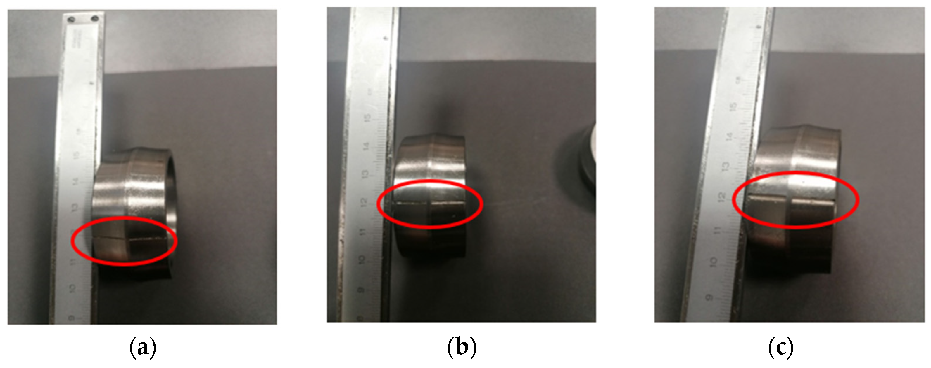
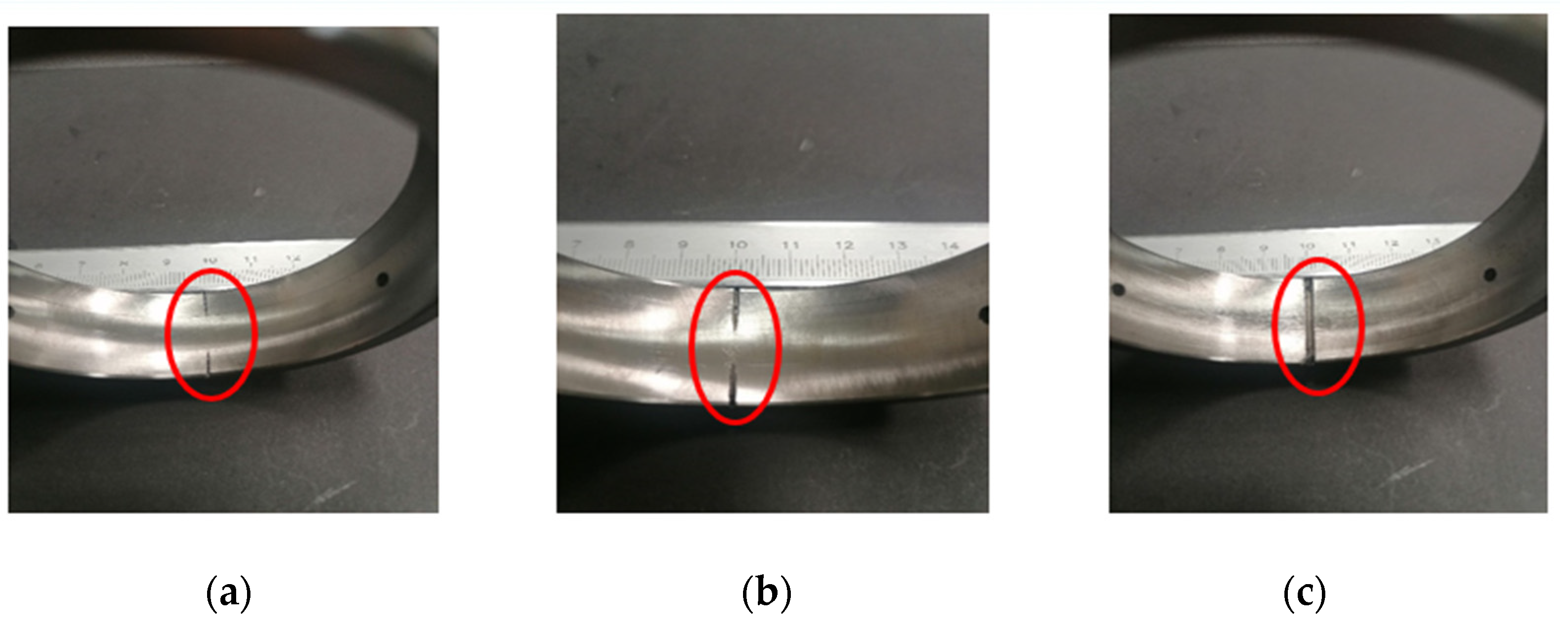
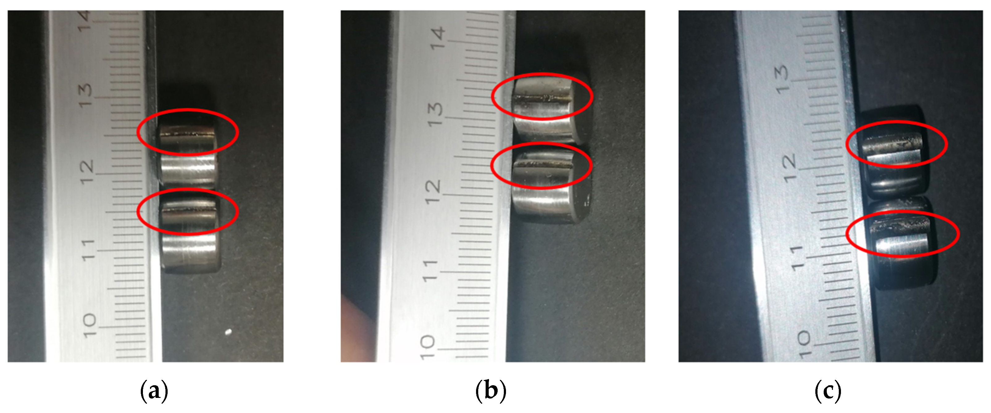
Artificial defects were engineered into the bearings using electrical discharge machining (EDM) to simulate typical faults in bearing component. This process ensured the controlled introduction of damage in various locations, such as the inner and outer races and the rollers, which are common sites for the origin of the defect. These artificially induced defects represented the initial signs of wear and tear, which can lead to more severe forms of degradation, such as spalling, cage collapse, and, ultimately, complete bearing failure. The precise nature of these defects is illustrated in Figure 3. This methodical induction of faults allowed for the creation of a realistic test environment to effectively evaluate diagnostic techniques and predictive maintenance strategies.

Electrical discharge machines (EDMs) can create artificial bearing defects, allowing for controlled testing and analysis of their performance under different conditions. EDMs can simulate common types of damage in real-world bearing applications, such as cracks or wear patterns, enabling a more accurate assessment of bearing durability and reliability. An artificial defect was created in the inner, outer, and rolling elements of the spherical bearing using an EDM, as mentioned in

Table 2. Dimensions of defective bearings in EDM experiments.

No	Bearing Part	Label Name	Diameter mm	Depth mm	Length mm
1	Inner Race Defect IRF	IRF0.5	0.5	0.3	23
	As shown in Figure 5	IRF1	1	0.5	23
		IRF2	2	1	23
2	Outer Race Defect ORF	ORF0.5	0.5	0.3	6.5
	As shown in Figure 6	ORF1	1	0.5	8.5
		ORF2	2	1	23
3	Spherical Element Defect RF	RF0.5	0.5	0.3	8.35
	As shown in Figure 7	RF1	1	0.5	8.35
		RF2	2	1	8.35

, for use in separate experiments and as shown in Figure 4.

2.4. The Alignment Procedure Using the FixturLaser XA System

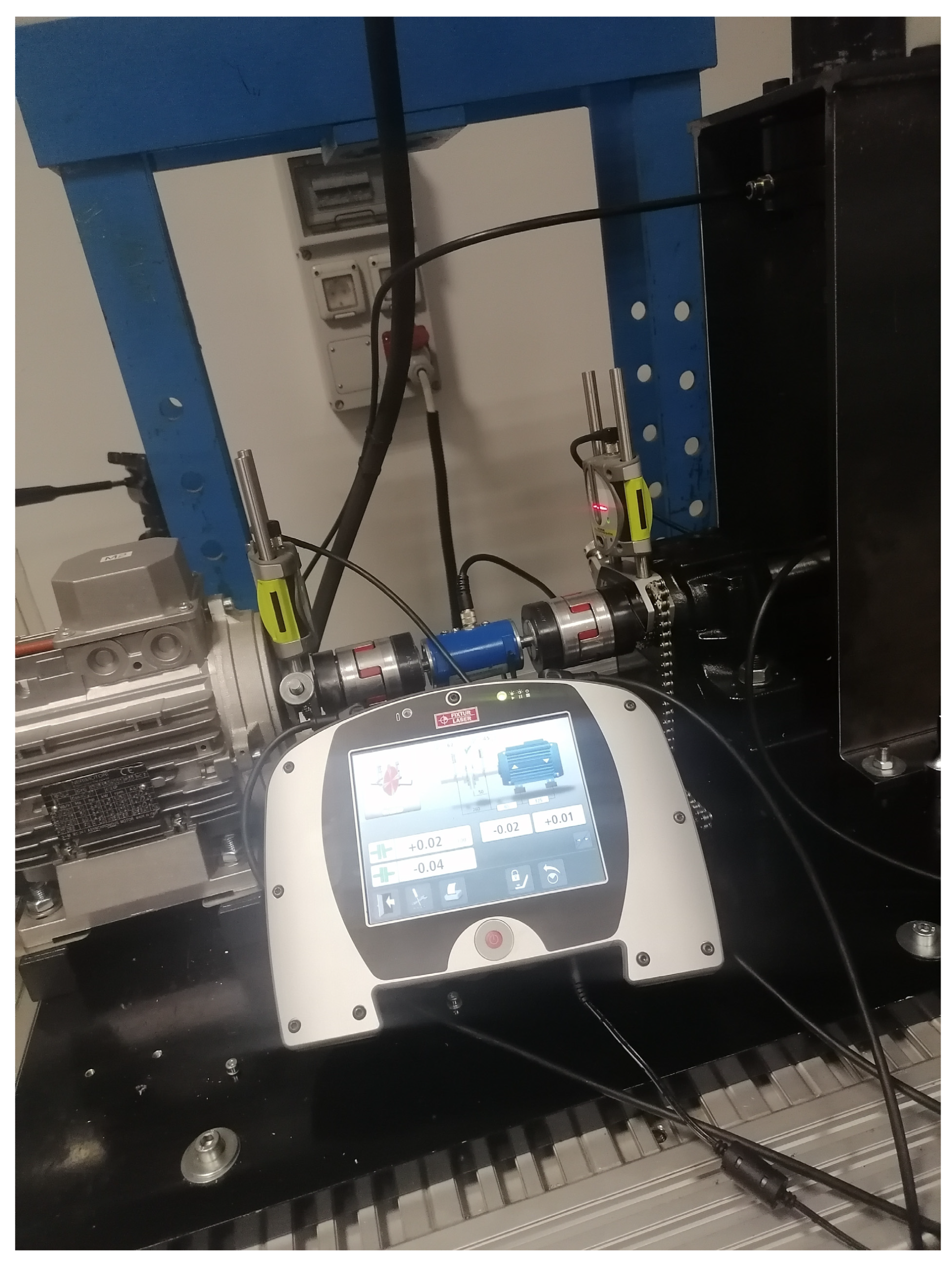
The FixturLaser XA system is commonly used to assess and correct misalignment. This method allows for the precise alignment of motor shafts within designated tolerances by adjusting the vertical and horizontal positions of the front and back pairs of the motor foot. The alignment process was performed using a tolerance table in the device manual. The Fixturlaser XA system uses two measurement units placed on each shaft, using the fittings provided by the system as illustrated in Figure 8. The system determined the relative distance between the two shafts in the two planes by rotating the shafts to various measuring points using bearings. The system received the input of the measurements taken from the bearing to the connection and motor feet. The Fixturlaser XA display provided precise data on the current alignment status and the motor position.

2.5. Hydraulic Load System

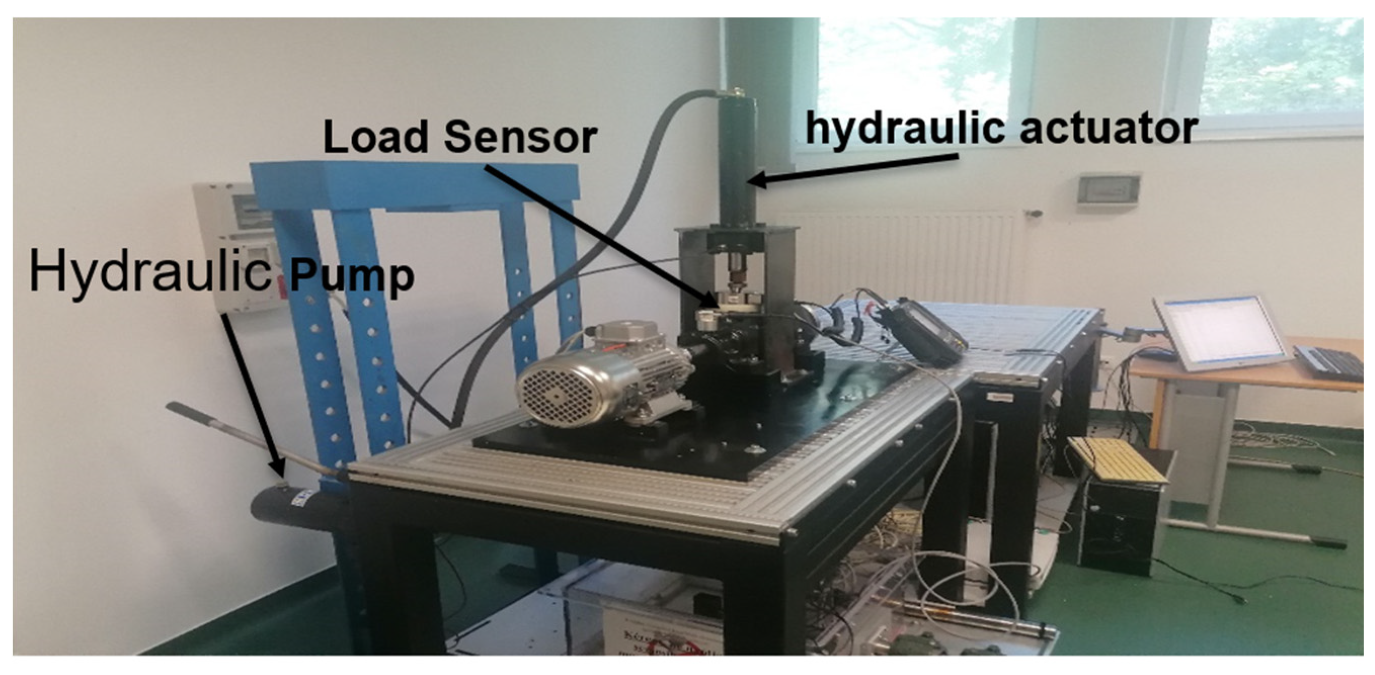
The loading system consisted of a hydraulic pump attached to a load frame structure and then connected to a hydraulic actuator. The hydraulic cylinder, which was the final component of this system, was used to apply pressure to the HBM C2 load sensor. This load sensor was designed to measure the force exerted by the hydraulic cylinder and provide feedback to the display, allowing the user to keep track of the amount of force applied, as illustrated in Figure 9 and Figure 10.

2.6. Vibration Measurement Device

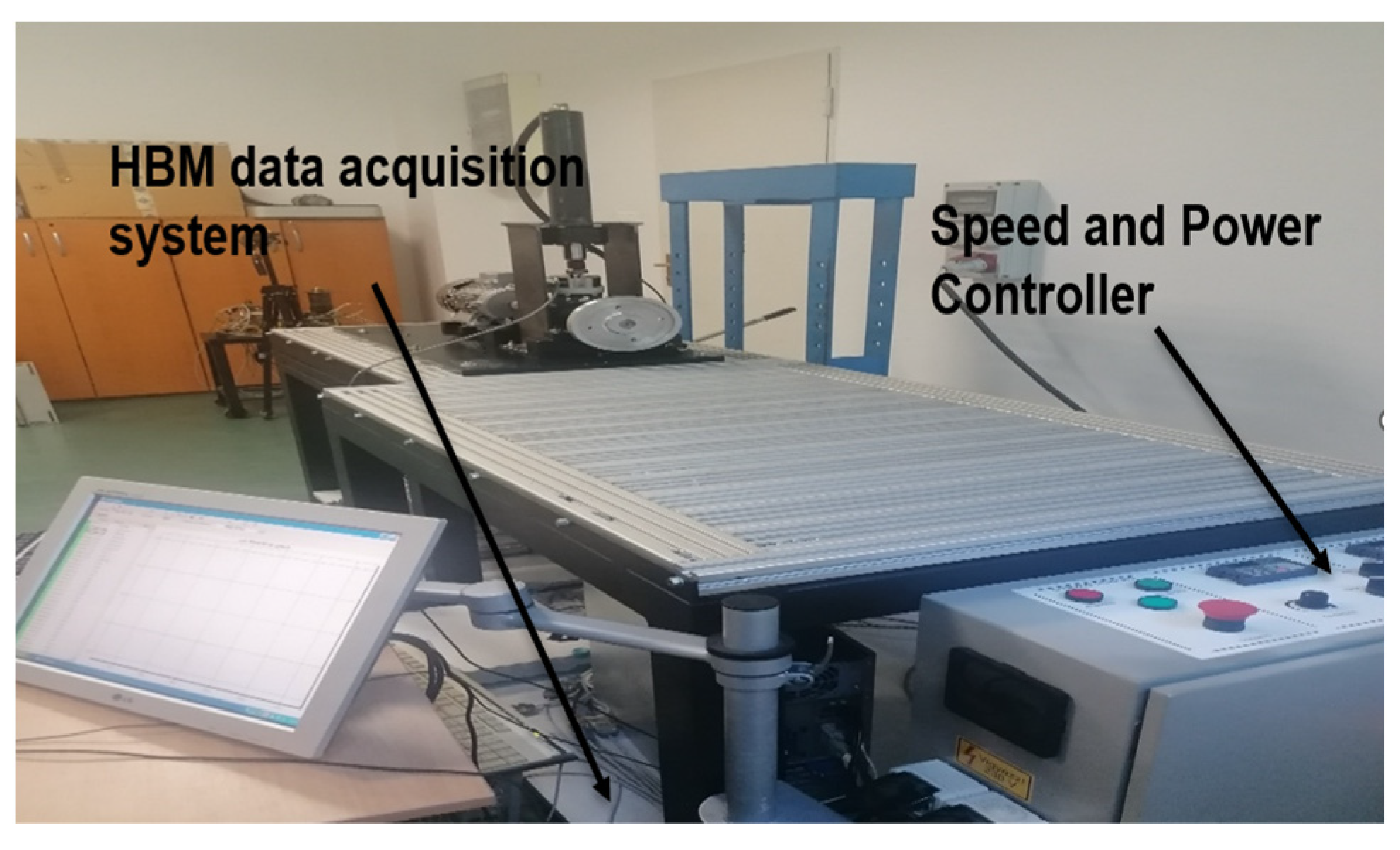
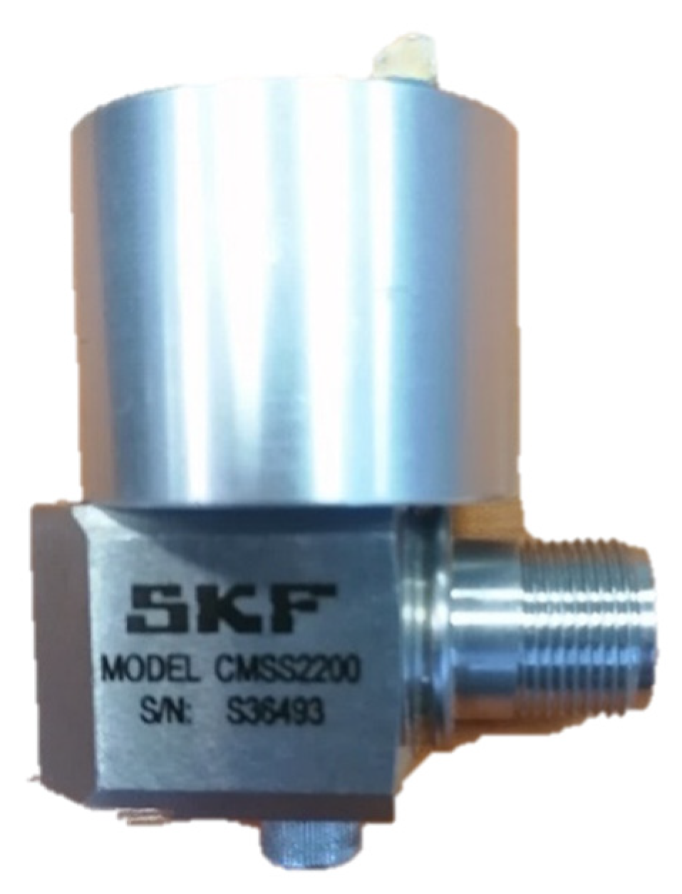
The test rig was driven over a DC motor through flexible coupling. This setup allowed for efficient and reliable monitoring and control of motor performance. The power and speed controller, shown in Figure 10, effectively regulated the motor’s operation. Additionally, using the non-contact SKF optical tachometer TMOT6, shown in Figure 11, provided accurate measurements of the motor’s rotational speed. The CMSS 2200 accelerometer, which has a sensitivity of 100 mV/g, was securely attached to the bearing housing using a magnetic component, making it suitable for various applications.

SKF Microlog CMX80, shown in Figure 12, is a valuable tool for machine health monitoring and predictive maintenance, particularly for research purposes. The comparative efficiency, accuracy, and reliability of SKF Microlog CMX80 in modern industrial environments underscore its advantages over other methods. Furthermore, the 100 mV/g sensitivity of the CMSS 2200 accelerometer enables it to measure vibrations in multiple applications, making it a versatile tool for detecting and monitoring vibrations in various systems. Combining the vibration measurement device and the power and speed controller provided an efficient and reliable means of monitoring and controlling motor performance.

2.7. Vibration Measurement Procedure

Extensive standardizations of the experimental apparatus were initiated before beginning any experimental pursuit. The machine operation was started for 15 min, during which the healthy test bearing was secured on the shaft, from which the vibration signals were collected. The electric motor was activated, and a speed controller was employed to regulate the speed of the shaft. A CMSS 2200 piezoelectric sensor or accelerometer was used to capture the vibration signals from the bearing housing connected to a magnetic base, as shown in Figure 13. Accelerometers are designed to measure mechanical motion and convert these data into analog signals, which are subsequently transmitted to a frequency analyzer. The FFT analyzer digitized the recorded signal, and the computer received and stored the discrete signal for subsequent analyses.

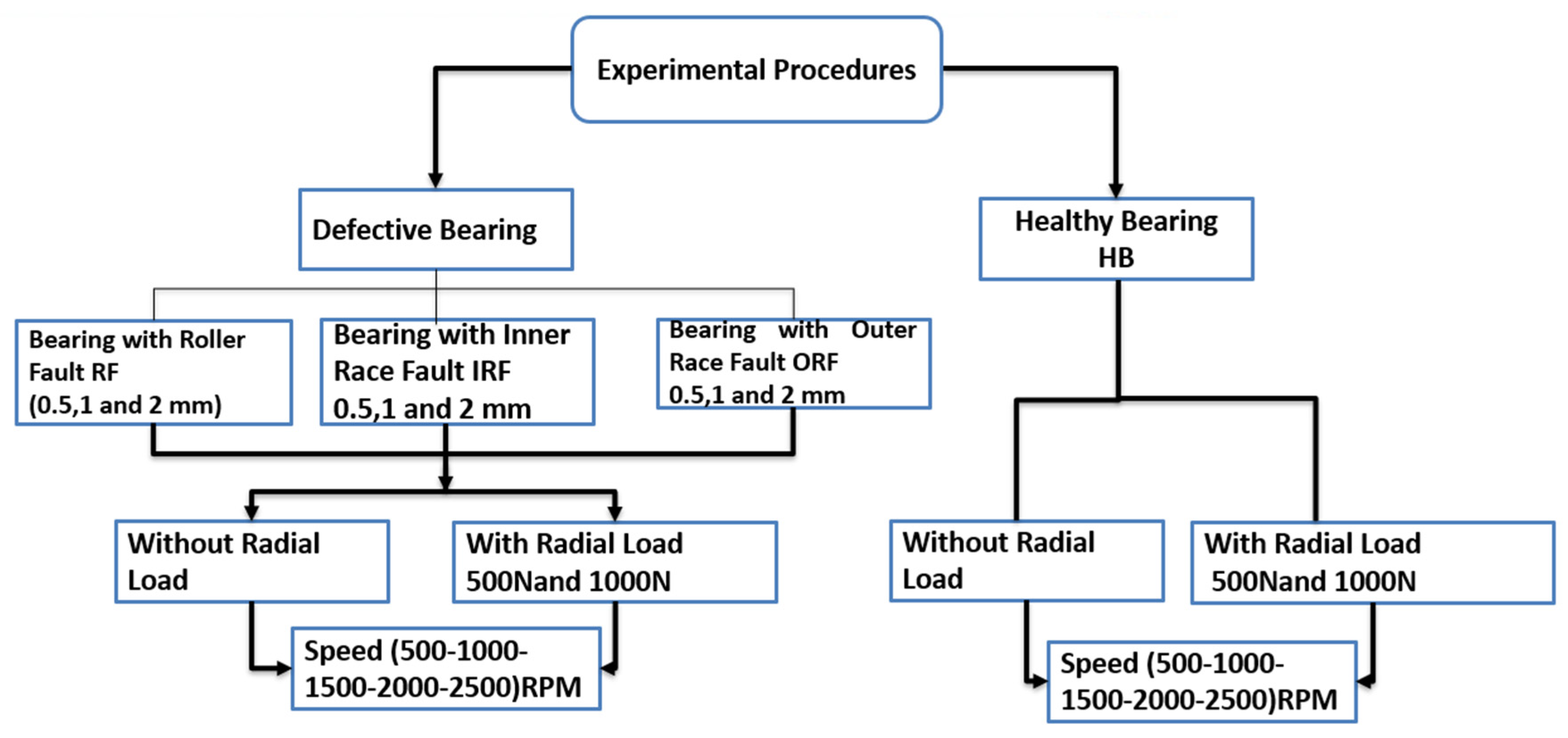
A new study conducted by [45].using cylindrical roller bearings highlighted the importance of sensor placement in accurately identifying bearing faults. The study emphasized that the same fault can cause variations in recorded signals at different places in the bearing housing, owing to the nature of vibration transmission. This fluctuation is explained by the uneven thickness and weakening of the vibration signal from the source, which results in variable vibration signals due to different levels of structural rigidity [15]. Research by [45] highlighted the significant influence of load and speed on the creation of defects. This study seeks to deepen our understanding of these effects to theoretically guide sensor placement and enhance the precision of bearing defect diagnosis precision under varying operational conditions. It is vital to understand the generation of structural vibration within the bearing housing and the transmission of fault excitation to determine the optimal sensor installation sites. The schematic in Figure 14 provides a structured approach to conducting experiments, with each path representing a different experimental condition. This allowed for extensive data collection and subsequent analyses. The results obtained from this procedure would be beneficial for predictive maintenance and bearing design as they would provide information on how different defects and loads affect bearing lifespan and performance.

For loaded and unloaded conditions, the bearings were tested at various speeds, ranging from 500 to 2500 RPM, broken down into three ranges: 500, 1000, 1500, 2000, and 2500 RPM. The load was measured instantaneously using a load sensor connected to the HBM Spider 8 and a computer with Catman v5 software to apply the exact load to the bearing housing.

The following procedures were used to collect healthy bearings:

• To begin collecting data, a healthy SFK 22209EK spherical roller bearing was installed into the bearing housing of the test rig.
• The level of the rig, the balance of the machine components, and electrical connections were tested.
• The accelerometer was connected to the SKF Microlog Analyser CMX80 using a cable after being magnetically attached to the bearing housing, as shown in Figure 15.
• Using a speed controller, the shaft was run at constant speeds of 500, 1000, 1500, 2000, and 2500 RPM.
• The SKF Microlog Analyser and accelerometer were used in both directions (vertical and horizontal) after 20 min of operation of the healthy bearing, with five rotation speeds on the test rig.
• The acceleration vibration signature was captured in the time domain in a frequency range of 10,000 HZ, and the frequency sampling was 25,600 HZ.
• Defective bearing parts, with an inner race, an outer race, and a spherical roller, were replaced for both loaded and unloaded conditions, and the bearings were tested at various speeds ranging from 500 to 2500 RPM.
• The hydraulic pump applied pressure to the load sensor during load scenarios. The sensor, connected to a data logger, precisely sent the load values to the Catman V5 software until the load reached the defined values of 500N and 1000N.
• The operation was carried out at different rotational speeds, ranging from 500 to 2500 RPM, for each load and unload situation. This procedure was implemented for every faulty component and undamaged bearing, as illustrated in Figure 14.
• Finally, vibration signatures were collected, as shown in Figure 15, and the data were transferred to a computer for data analysis, where the Analysis and Report Manager (ARM) version 2.4 software was installed.

2.8. Transfer Learning Model

Data Preprocessing

Once the raw data were collected, they underwent a preprocessing stage, where they were first converted into a time–frequency representation using a scalogram filter bank. This conversion is crucial for capturing the nonlinear and non-stationary nature of bearing signals. Data are categorized into a coding scheme in

Table 3. Coding scheme for each case study with different loads and rotation speeds.

Load	500 RPM	1000 RPM	1500 RPM	2000 RPM	2500 RPM
Load 0	L0-RS1	L0-RS2	L0-RS3	L0-RS4	L0-RS5
Load 500 N	L1-RS1	L1-RS2	L1-RS3	L1-RS4	L1-RS5
Load 1000 N	L2-RS1	L2-RS2	L2-RS3	L2-RS4	L2-RS5

, where each combination of load and rotation speed is represented as follows.

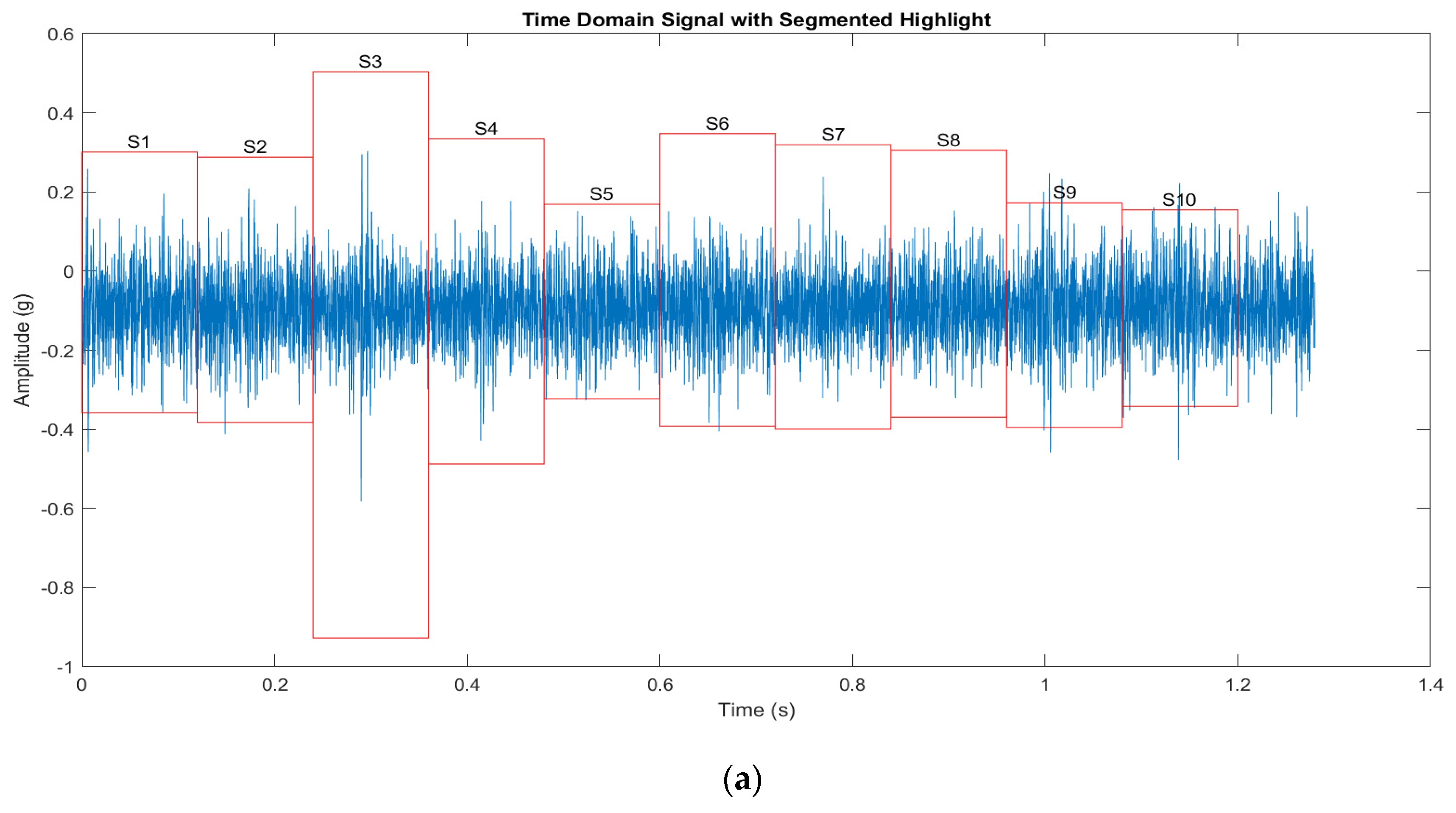
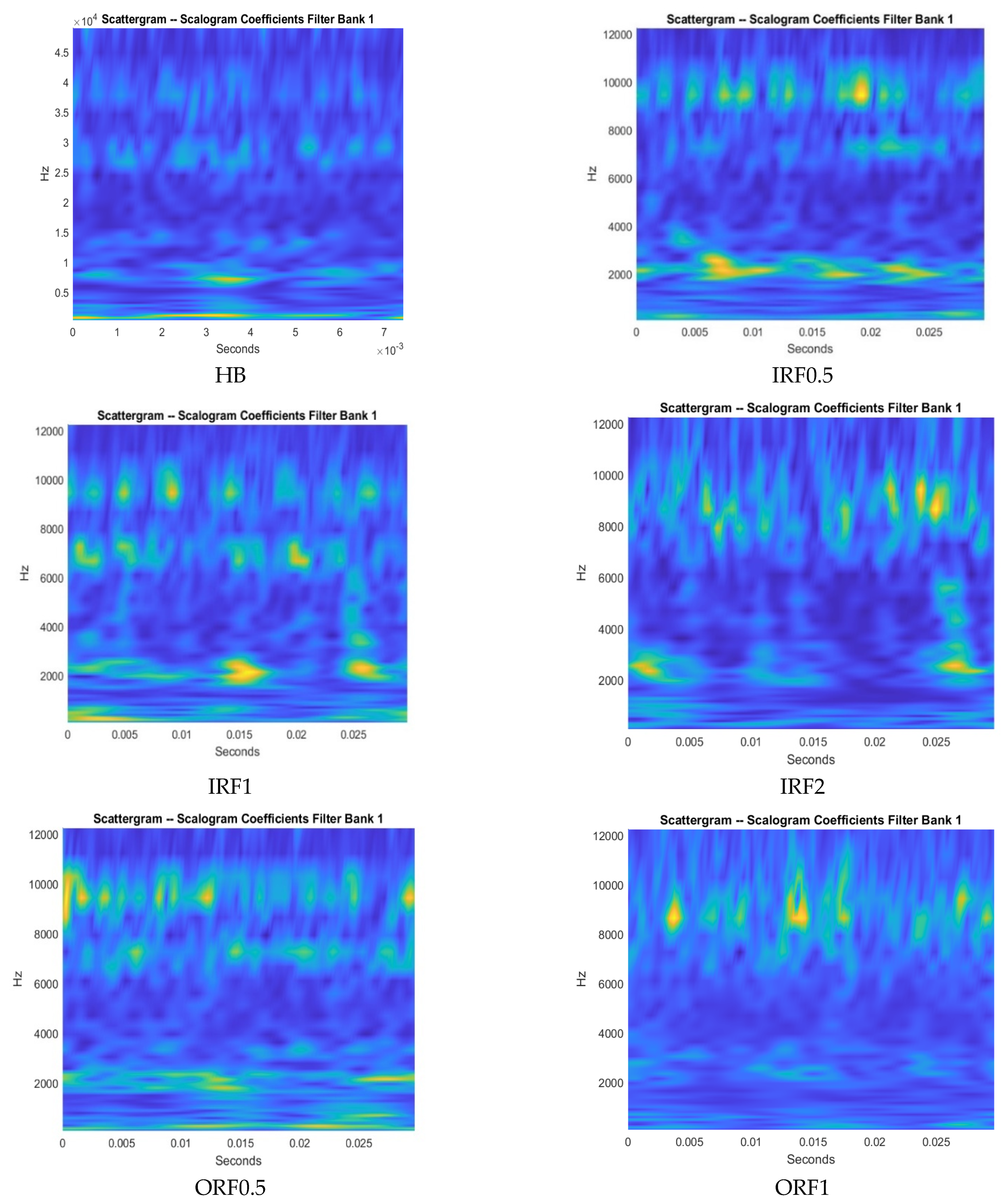
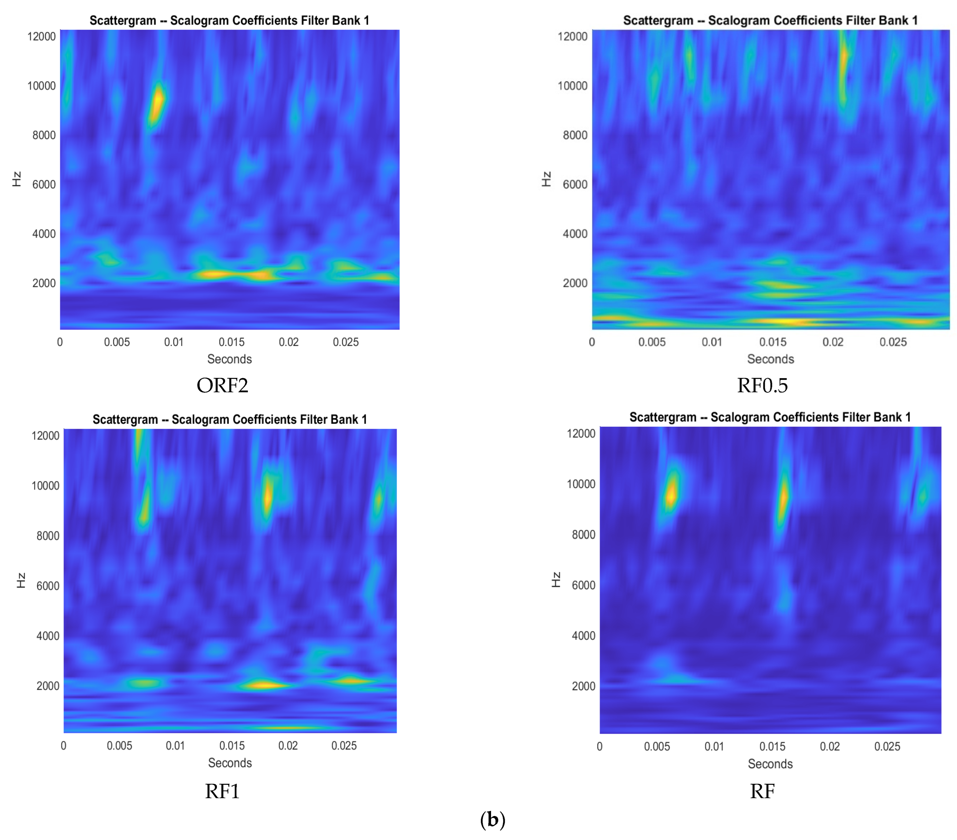
The method was developed to convert vibration signals into images for processing using scalogram filter bank 1. The processed signals were then segmented according to the rotational speed of the bearings. This segmentation ensured that each image generated from the scalogram corresponded to a full bearing rotation, which was essential for capturing the complete behavior of the bearing within each operational cycle (

Table 4. N values for each rotation speed.

N Bearing Speed (in RPM)	N is the Number of Sampling Points for One Cycle
500	3072
1000	1536
1500	1024
2000	768
2500	614.4

), as illustrated in Figure 16.

The total number of samples was 32,768

To calculate the number of sampling points for one cycle N, the formula is as follows:

$$N=\frac{fs\times 60}{n}$$

(1)

where

• fs denotes the sampling frequency (Hz),
• n is the bearing speed (in RPM),
• The time is 1.28 s,
• The sampling frequency (in Hz), totaling 25,600.

The Scattergram Filter Bank 1 image was generated using MATLAB’s scattergram function, specifically designed for wavelet-scattering representations. The function was invoked as follows: scattergram (sf, U, filterBank, 1), where sf represents the wavelet scattering object, and U denotes the cell array of wavelet scattering coefficients [46].

In the context of diagnosing and detecting faults in rolling element bearings, labels play a crucial role in identifying the type and size of defects present within bearing components. Each label name corresponds to a specific defect type and size, facilitating precise categorization and analysis.

• The label “HB” stands for healthy bearing, indicating a bearing that is free from defects and operates under normal conditions.
• Outer race defect (ORF): The label “ORF”, followed by a numerical value, denotes a defect on the outer race of the bearing, with the number indicating the diameter of the defect in millimeters. For instance, “ORF0.5” signifies a defect on the outer race with a diameter of 0.5 mm, “ORF1” for a 1 mm defect, and “ORF2” for a 2 mm defect.
• Inner race defect (IRF): Similarly, “IRF” labels are used to denote defects on the inner race of the bearing. “IRF0.5” refers to a defect with a 0.5 mm diameter, “IRF1” to a 1 mm defect, and “IRF2” to a 2 mm defect.
• Spherical element defect (RF): The label “RF” is used for defects on the spherical elements (rollers) of the bearing. “RF0.5” indicates a defect of 0.5 mm diameter, “RF1” for a 1 mm diameter defect, and “RF2” for a 2 mm diameter defect.

The segmented scalograms were adjusted in size or padded to match the input dimensions specified by ResNet-101, VGG16, VGG19, ResNet-18, and ResNet-50 architectures. The standard input size for the VGG16 and VGG19 models was 224 × 224 pixels, which was applied to DenseNet-201. On the contrary, TL_ResNet-101 often required an input dimension of 256 × 256 pixels. Resizing or padding is essential to guarantee that the images meet each network’s specific input layer criteria. Furthermore, the pixel values of the images were normalized across all models to standardize the scale of the input data. This is advantageous for the learning process because it guarantees uniformity. Subsequently, the prepared photos were partitioned into training, validation, and testing sets, a customary machine learning approach to evaluate the model’s performance and ability to apply knowledge to unfamiliar data. The research utilized pre-trained models such as ResNet-101, VGG16, VGG19, ResNet-18, and ResNet-50. The upper layers of these models were eliminated to customize them for transfer learning, making them suitable for the precise classification of bearing defects. In the transfer learning configuration, additional top layers were incorporated into each model to classify bearing defects. In the early layers of TL_ResNet-101, four additional models (VGG-16, VGG19, ResNet-18, and ResNet-50) were kept fixed to retain the acquired features from the pre-training stage, 2.8.2 Model Training and Evaluation.

The model was compiled using an appropriate optimizer loss function and metrics tailored to the classification task. The system was then trained using the training and validation sets to monitor performance and adjust as needed. The model was trained using MATLAB R2023, with the computer specifications listed in

Table 5. Computer specification.

Operating System	Windows 10 Pro for Workstations 64 Bit
Processor	Intel(R) Xeon(R) W-2245 CPU @ 3.90 GHz (16 CPUs), ~3.9 GHz
Installed RAM	64.0 GB
GPU	NVIDIA Quadro RTX 4000

.

Finally, the performance of the model was evaluated using a test set. Relevant metrics were calculated to quantify the model’s accuracy, precision, recall, and F1 score, among others, to fully understand its diagnostic capabilities, as shown in Formulas (2)–(4).

$$\mathrm{Accuracy}=\frac{TN+TP}{TN+FP+TP+FN}$$

(2)

$$\mathrm{Precision}=\frac{TP}{TP+FP}$$

(3)

$$\mathrm{Recall}=\frac{TP}{TP+FN}$$

(4)

$$F1\mathrm{Score}=2\ast \frac{\mathrm{Precision}\ast \mathrm{Recall}}{\mathrm{Precision}+\mathrm{Recall}}$$

(5)

$$\mathrm{Specificity}=\frac{TN}{TN+FP}$$

(6)

where TP is the true positive, TN is the true negative, FP is the false positive, and FN is the false negative.

The model evaluated the effectiveness using the IMS public data set (Intelligent Maintenance Systems), and the data for the Intelligent Maintenance Systems (IMS) study were generated using a test rig with four bearings installed on a shaft. Lee et al. (2007) conducted this study previously. This study used a test apparatus equipped with four Rexnord ZA-2115 double row bearings attached to a shaft [35]. The bearings were greased under pressure and the rotational speed was maintained at 2000 RPM. High-sensitivity quartz ICP accelerometers (model PCB 353B33) were placed on the bearing housing to collect data. The IMS data set was made up of three separate data sets that reflect unique test-to-failure studies. Each data set consisted of 20,480 data points. Test 1 revealed the presence of inner race faults in bearing 3 and roller element defects in bearing 4. Bearings 1 and 3 had defects in the outer race, as shown in Figure 17c–e. Vibration data were acquired at 20 min intervals using a National Instruments DAQCaRFTM-6062E instrument. Data were collected formally using the National Instruments LabVIEW version 8.5 software [35]. Figure 17b illustrates the Rexnord ZA-2115 double row bearings on a single shaft. The bearings consisted of 16 rollers in each row.

Table 6. IMS test setup and results for three different sets of experiments.

Test No.	Type of Bearing	Arrangement of the Accelerometer on the Bearing	Type of Fault at the End of the Test	Sensor
1	Rexnord ZA-2115	Bearing 3—Ch 5 and 6; Bearing 4—Ch 7 and 8;	Bearing 3: Inner race defect (IRF) Bearing 4: Roller element defect (RF)	2 accelerometers per bearing (x- and y-axes)
2	Rexnord ZA-2115	Bearing 1—Ch 1;	Bearing 1: Outer race failure	1 accelerometer per bearing
3	Rexnord ZA-2115	Bearing 3—Ch 3;	Bearing 3 Outer race fault	1 accelerometer per bearing

presents the test setups and results of the three experiments with Rexnord ZA-2115 bearings. Table 6 includes the number of tests, the arrangement of accelerometers in each bearing, and the condition of the bearings after the tests were completed.

3. Results and Discussion

This section presents the results of the experiments conducted with SKF 2209EK spherical roller bearings and the model’s ability to classify and predict various bearing faults under different operational conditions, transfer learning, and ResNet-101 in bearing fault diagnosis, with improved accuracy and reliability compared to traditional methods.

3.1. Results of the Experiment

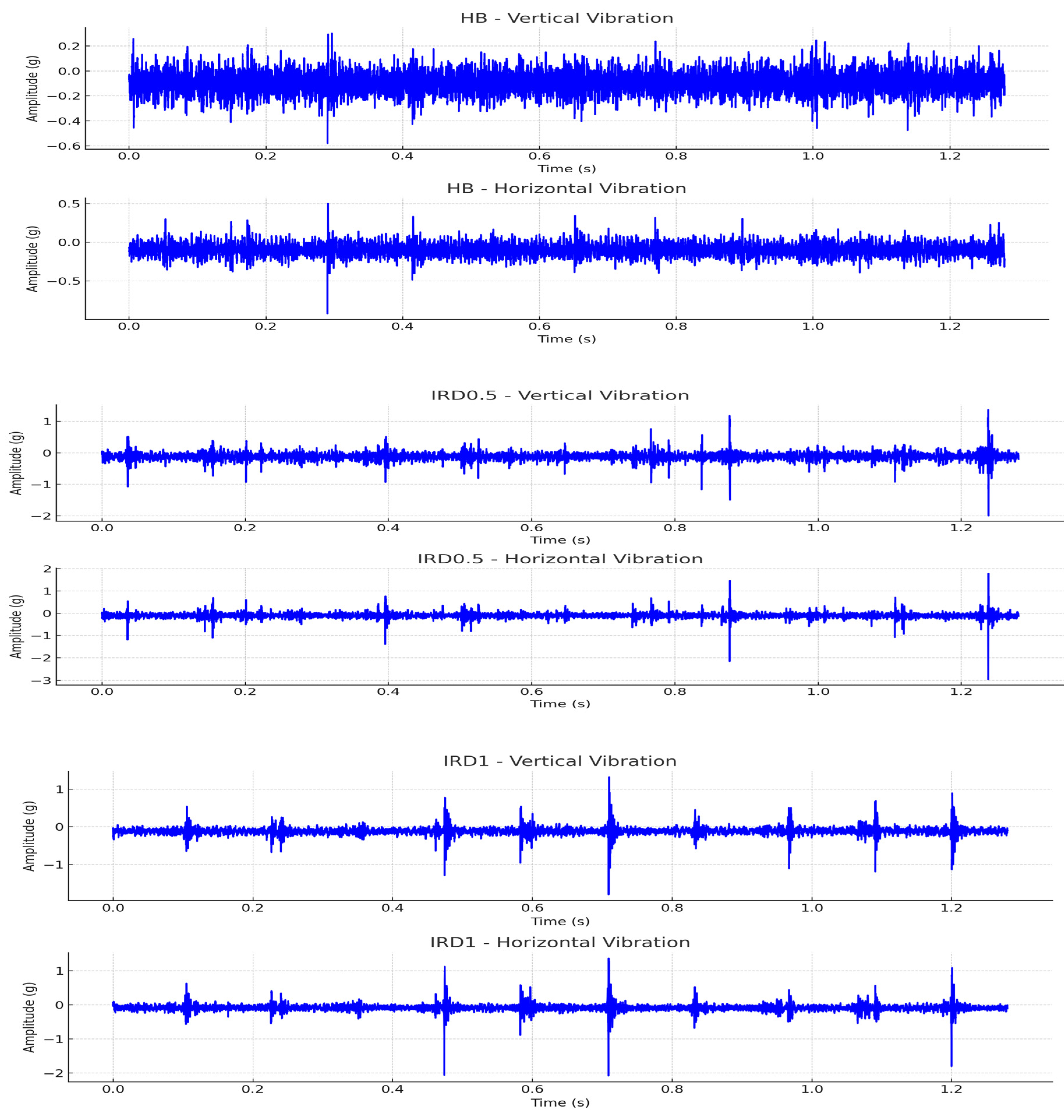
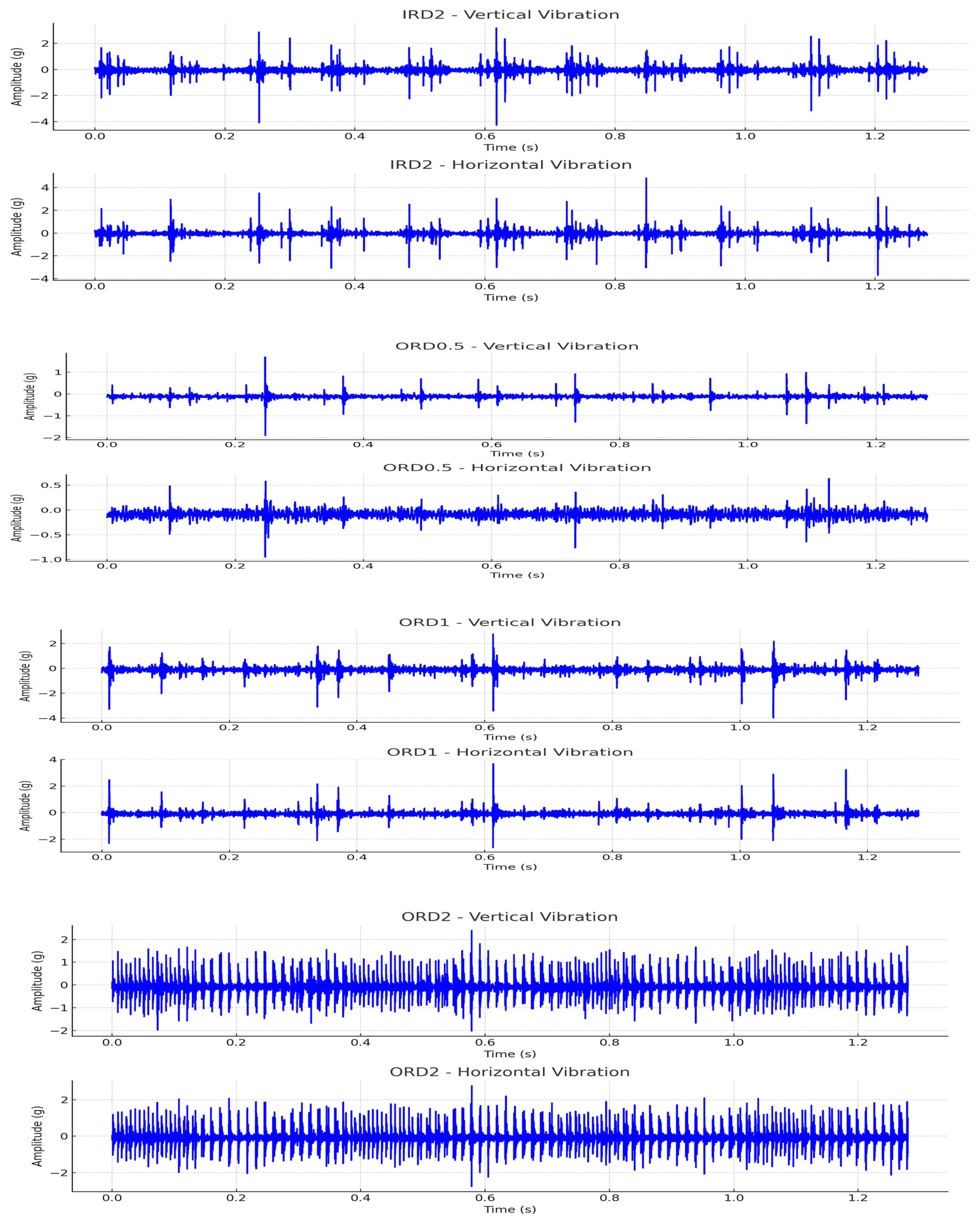
The load and speed variations significantly affect the vibration signatures of the bearings. Faults in different parts of the bearings (such as the inner race, outer race, and spherical roller) alter the vibration patterns, and these alterations are more pronounced at higher speeds due to increased dynamic effects on the measured data in the vertical (V) and horizontal (H) directions. Raw vibration data for three cases, L0-RS1, L1-RS1, and L2-RS1, in the vertical and horizontal directions, are presented in Figure 18. The example of a time domain data scenario for one case is illustrated in Figure 18, which shows distinct vibration characteristics on the vertical and horizontal axes for healthy and defective bearings, where each image represents the vertical amplitude in the upper layer and the horizontal amplitude under it. Our experiments reveal that faults in different bearing components (inner race, outer race, spherical roller) significantly alter vibration patterns. This effect becomes even more pronounced at higher speeds due to increased dynamic forces. It was observed that there is some similarity between the vertical and horizontal amplitudes. Key observations include variations in amplitude and any notable patterns or anomalies in vibration data. These vibration data exhibit distinct vibration characteristics along both the vertical and horizontal axes.

3.2. Transfer Learning Model Results

In deep learning, particularly in the context of transfer learning, selecting hyperparameters is critical for determining a model’s effectiveness and efficiency.

Table 7. Hyperparameters for transfer learning.

Hyperparameter	Value
Optimizer	Adam
L2 regularization	1 × 10−4
Mini batch size	32
Initial learning rate	1 × 10−4
Max epochs	15

presents a detailed overview of the hyperparameters selected to implement transfer learning in ResNet-101, VGG16, VGG19, ResNet-18, and ResNet-50 architecture. This table is pivotal because it outlines the specific settings used to fine-tune the pre-trained ResNet-101, VGG16, VGG19, ResNet-18, and ResNet-50 models for the task at hand, which, in this case, is likely related to bearing fault detection.

3.2.1. Case Study 1 (L0)

The confusion matrices allowed us to analyze the performance of ResNet-101, VGG16, VGG19, ResNet-18, and ResNet-50 on the experimental data in more detail. By examining off-diagonal elements, we can identify which classes are often misclassified and gain insight into potential areas for improvement. Comparing this confusion matrix with previous ones helps us to understand whether the model’s performance has improved or deteriorated over time. Ten labels were used to train each model, corresponding to different classes or types of bearing faults. HB was used for healthy bearing, ORF was used for outer fault, IRF was used for inner race fault, and RF was used for roller fault, the numbers (0.5, 1, 2) indicating the size of the fault. The confusion matrices provided show the performance of the classification model in five different data sets or under different conditions. True classes appear to represent the health status of bearings with varying degrees of defects in the inner race, outer race, and rollers. Figure 19 illustrates Case Study 1 for five rotation speeds and a clear increase in data samples, as indicated by the increasing numbers along the diagonal. This increase typically represents the model’s performance better and can lead to more accurate predictions.

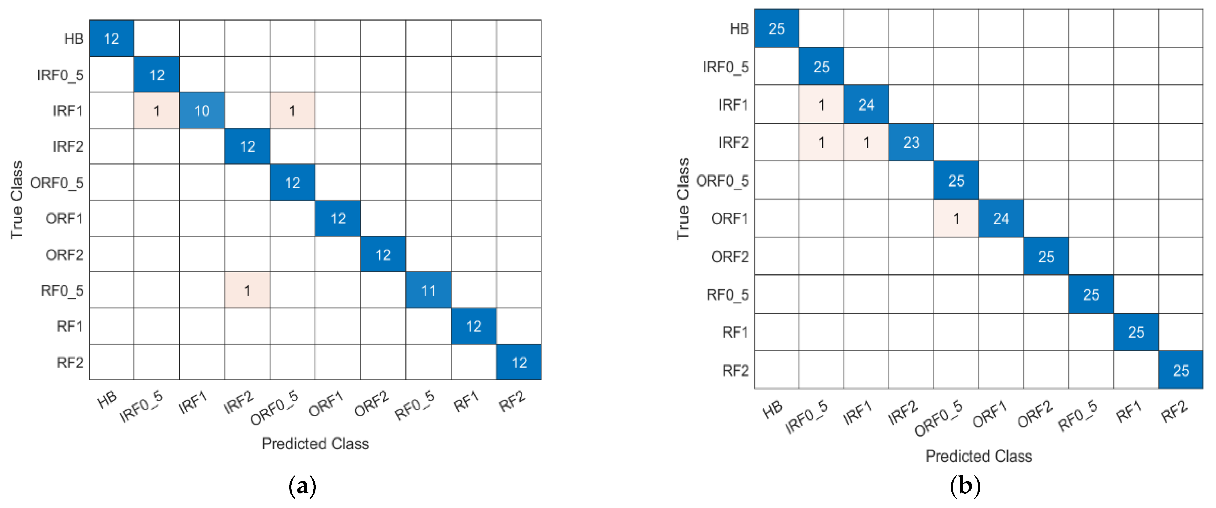
The confusion matrices illustrate the classification results of a machine learning model designed to detect various bearing problems. The initial matrix demonstrates a predominantly elevated level of precision, although it occasionally shows a misclassification between IRF1 and other fault classifications. The second matrix exhibits superior precision, demonstrating enhanced model prediction capabilities. Within the third matrix, there is discernible ambiguity about the distinction between ORF0.5 and IRF2, indicating a potential scope for enhancing the model. The fourth matrix demonstrates robust performance, albeit with some misclassifications, particularly between IRF1 and HB. The final matrix demonstrates the highest level of classification accuracy with very few errors. This indicates a robust model for detecting faults; however, there are some instances when IRF 0.5 and RF 0.5 are incorrectly classified. These matrices are vital instruments for evaluating the accuracy of problem detection, which is crucial for the upkeep and dependability of mechanical systems.

Table 8. Training accuracy (%) for Case Study 1.

Diagnostic Model	L0-RS1	L0-RS2	L0-RS3	L0-RS4	L0-RS5
TL_VGG-16	80	91.60	93.68	93.33	93.20
TL_VGG-19	95	95.20	89.21	95	95.47
TL_ResNet-18	96.17	96.80	95.26	95	95.16
TL_ResNet-50	97.50	97.60	94.21	96.20	96.56
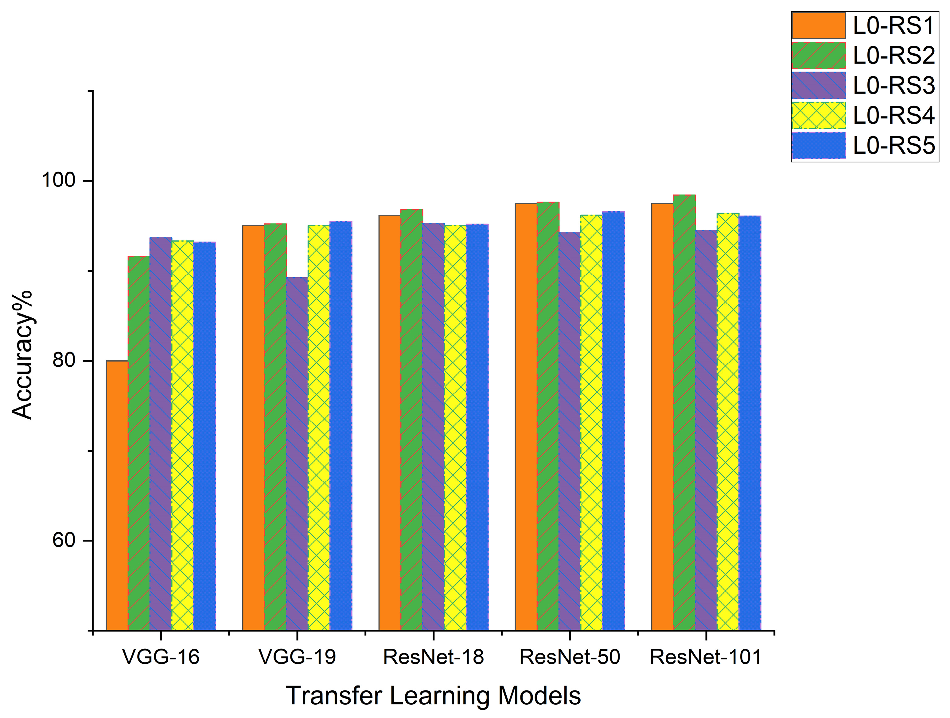
TL_ResNet-101	97.50	98.40	94.47	96.40	96.09

presents the training accuracy of the four diagnostic models TL_VGG-16, TL_VGG-19, TL_ ResNet-18, TL_ResNet-50, and TL_ResNet-101 across different rotational speed scenarios (RS1 to RS5) under no load (L0) conditions.

The TL_VGG-16 model shows varied performance at different speeds, with the highest accuracy observed at L0-RS1 (93.68%) and the lowest at L0-RS2 (80%). The fluctuation in accuracy suggests that, while TL_VGG-16 is generally effective, its performance may be affected by changes in the rotational speed, and the TL_VGG-19 model consistently demonstrates high accuracy. TL_VGG-19 excels, particularly at L0-RS2 (95.20%) and L0-RS5 (95.47%). Its performance indicates robustness across the range of speeds, suggesting an adequate adaptation of the model to varying conditions without load. The TL_ResNet-101 model shows an impressive ability to maintain high accuracy, peaking at L0-RS2 (98.40%). The consistency in performance across speeds indicates that TL_ ResNet-50 is highly reliable under no-load conditions; TL_ResNet-101 exhibits the highest accuracy among the models, demonstrating exceptional proficiency in fault diagnosis under no-load conditions. The graph in Figure 20 shows the training accuracy of each diagnostic model (VGG-16, VGG-19, ResNet-18, ResNet-50, and ResNet-101) under no-load conditions.

The accuracy percentages for each model were plotted for five different study repetitions (L0-RS1–L0-RS5). This graph helps us to understand how each model performs without load, indicating its robustness and reliability under ideal conditions. Variations across repetitions indicate the consistency of each model. The results highlight the importance of selecting an appropriate model based on operational conditions. The high accuracy of TL_ResNet-101 with no load at different speeds makes it preferable for fault diagnosis in these scenarios. Figure 20 presents the training accuracy of various transfer learning models across different rotational speed scenarios under no-load conditions. Models such as TL_VGG-16, TL_VGG-19, TL_ResNet-18, TL_ResNet-50, and TL_ResNet-101 are evaluated. The accuracy varies between different speeds, with TL_ResNet-101 achieving the highest accuracy at L0-RS4. The graph in Figure 20 illustrates the training accuracy of each model, which helps us to understand their performance and robustness under ideal conditions. The results underscore the importance of choosing the right model for specific operational conditions, with TL_ResNet-101 being preferred for fault diagnosis in no-load scenarios due to its high accuracy.

3.2.2. Case Study 2 (L1)

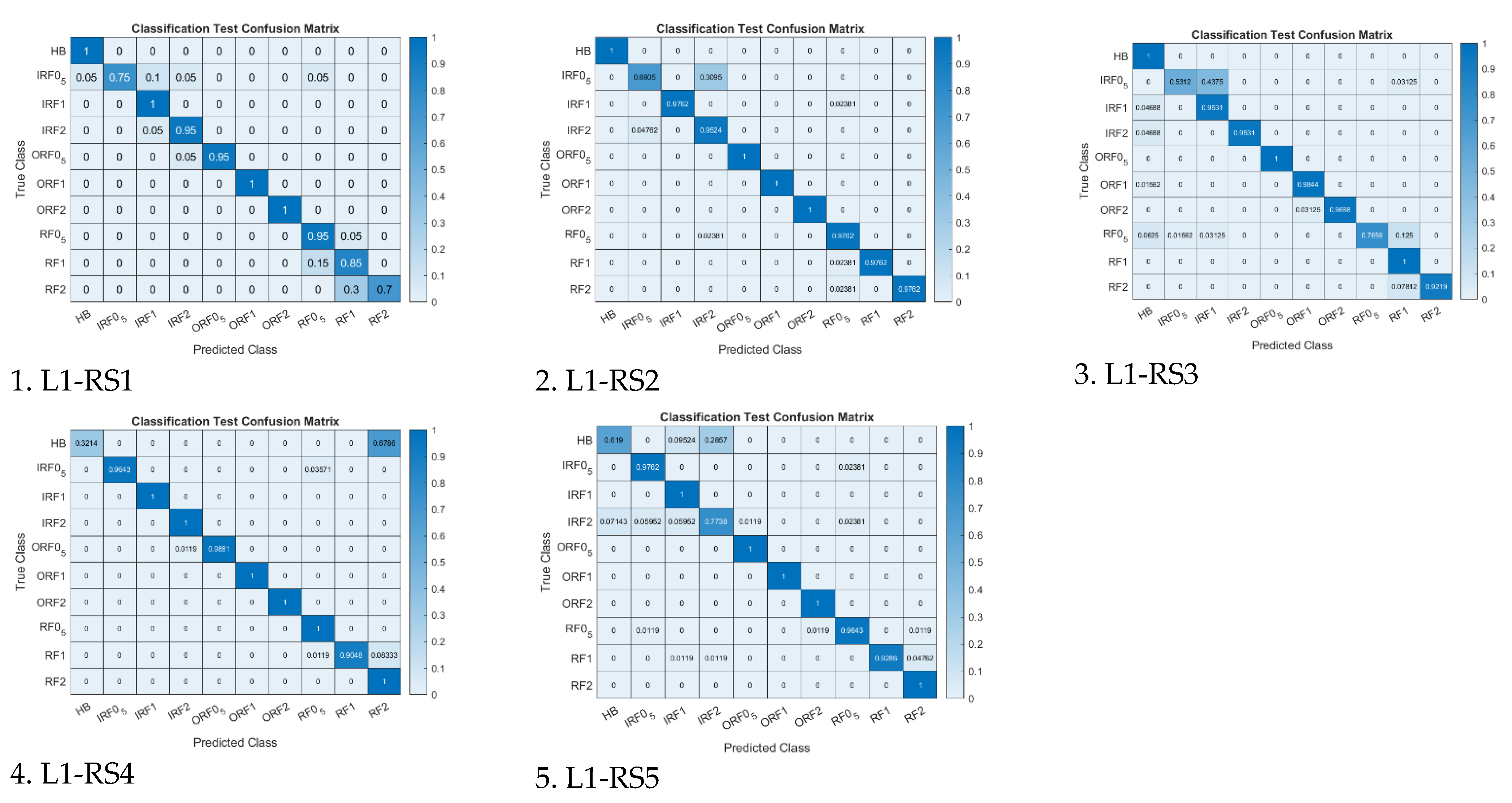
The matrices show that the model generally has high accuracy, as shown in Appendix A, from 1 to 5, with most predictions falling on the diagonal for classes representing healthy bearings and those with varying fault degrees. However, certain types of faults, particularly those with minor defects, exhibit more frequent misclassifications, indicating a challenge for the model to differentiate between subtle fault characteristics. Despite the high precision, some consistent confusion between closely related fault types (e.g., RF1 and RF2) suggests that the model may struggle to distinguish between similar fault severities. This is particularly evident in classes like RF0.5 and ORF0.5, which may share similar vibration signatures or extracted features, leading to misclassification.

Table 9. Training precision (%) for Case Study 2 (load is 500 N).

Diagnostic Model	L1-RS1	L1-RS2	L1-RS3	L1-RS4	L1-RS5
TL_VGG-16	95.67	79.60	93.44	92.60	90.47
TL_VGG-19	95	93.60	92.60	90.40	91.09
TL_ResNet-18	94.17	93.20	92.90	91.80	92.34
TL_ResNet-50	95.50	93.60	94	91.40	91.12
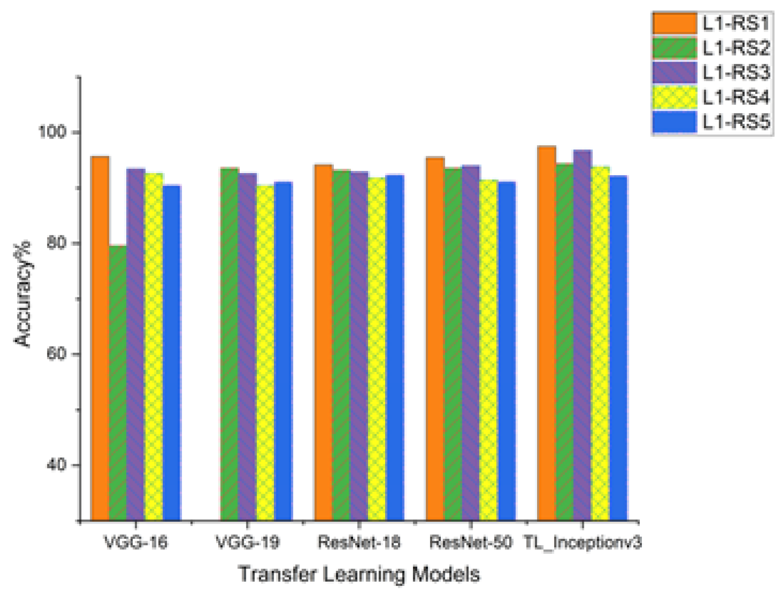
TL_ResNet-101	96.67	94	96.80	93.80	92.19

illustrates the training accuracy percentages for different transfer learning models applied to Case Study 2, where the load condition is 500N. Models include variations in VGG and ResNet architecture, specifically VGG-16, VGG-19, ResNet-18, ResNet-50, and ResNet-101. The performance is evaluated under five run scenarios (L1-RS1 to L1-RS5). The ResNet-101 model shows the highest accuracy in most scenarios, particularly excelling in L1-RS3 with a 96.80% accuracy rate. VGG-16, while showing the lowest accuracy in L1-RS2, performs consistently well in other scenarios. Data indicate that while all models are highly effective, specific models such as ResNet-101 may be more suitable for this diagnostic task under the given load condition.

The graph in Figure 21 illustrates the training accuracy percentages of five different transfer learning models in five separate runs for Case Study 2, under a load of 500N. Models tested include VGG-16, VGG-19, ResNet-18, ResNet-50, and ResNet-101. Each bar represents a model’s accuracy in a particular run, with colors denoting different runs (L1-RS1 through L1-RS5). The graph in Figure 21 shows that ResNet-101 generally achieves the highest accuracy on most runs, while VGG-16 and VGG-19 exhibit some variability. This visual representation helps to compare the consistency and reliability of each model’s performance in the given scenario.

3.2.3. Case Study 3 (L2)

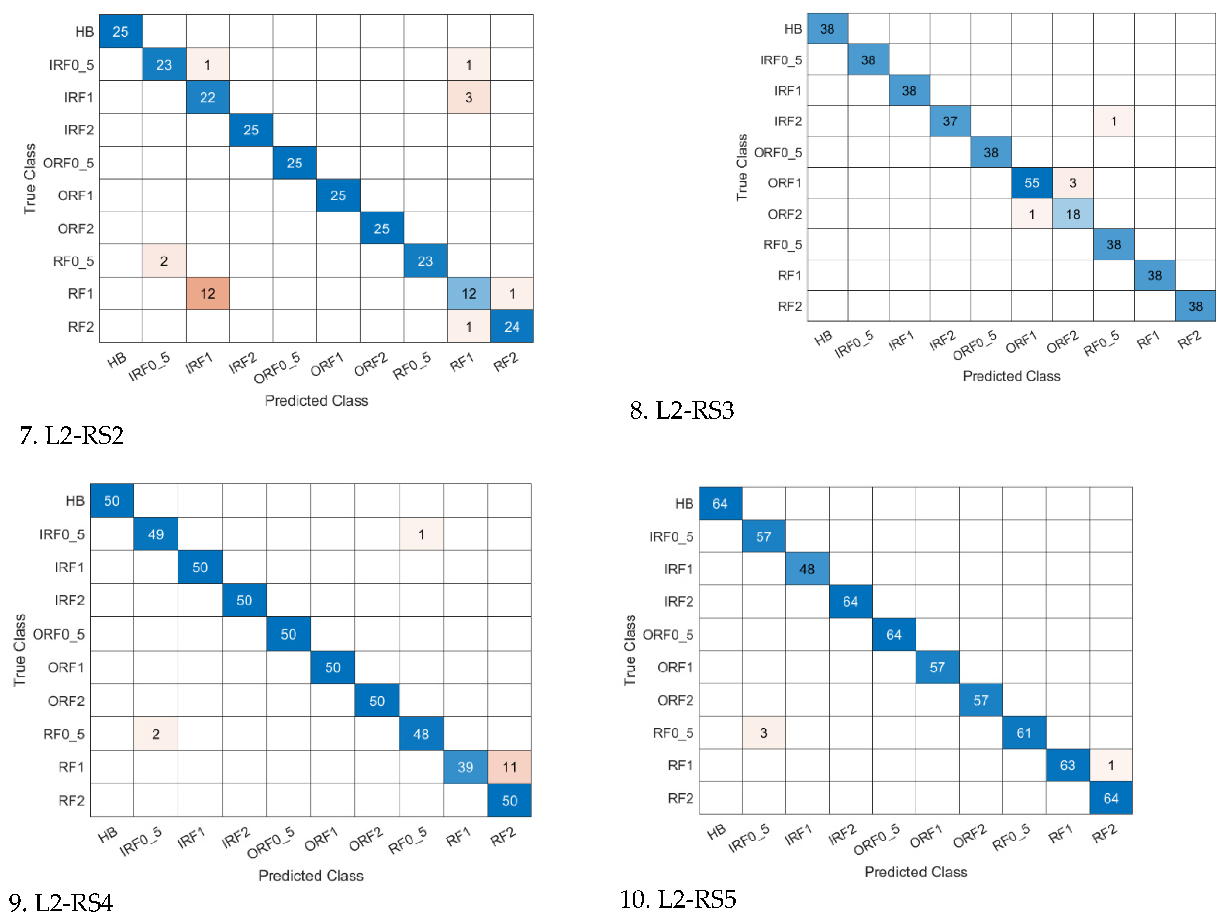
The accuracy of the model can be observed through the high number of true positives along the diagonals of the matrices, as illustrated in Appendix A, from 6 to 10. However, some consistent misclassifications are notable, particularly between certain fault classes with similar characteristics, such as RF0.5, RF1, IRF0.5, and HB, where the model seems to confuse one for the other. This pattern suggests that the model may benefit from further refinement in its ability to discern subtle differences between fault types. Despite the high accuracy, misclassifications highlight specific areas for improvement, such as feature engineering, data augmentation, and even re-visiting the model architecture. Fine-tuning the model to address these misclassifications is crucial to enhance its diagnostic performance and reliability in real-world applications for fault detection in rolling element bearings.

Table 10. Training accuracy (%) for Case Study 3 (Load is 1000 N).

Diagnostic Model	L1-RS1	L1-RS2	L1-RS3	L1-RS4	L1-RS5
TL_VGG-16	90.83	80	88.42	83.60	90.31
TL_VGG-19	85.83	81.20	90.29	86.60	97.84
TL_ResNet-18	95.83	91.60	98.16	96.15	99.17
TL_ResNet-50	96.17	90.80	97.64	97.20	98.01
TL_ResNet-101	97.50	93.20	98.95	98.60	99.34

presents the training accuracy of the five diagnostic models, TL_VGG-16, TL_VGG-19, TL_ResNet-18, TL_ResNet-50, and TL_ResNet-101, in different rotational speed scenarios (RS1–RS5) under a load condition of 1000 N (L2).

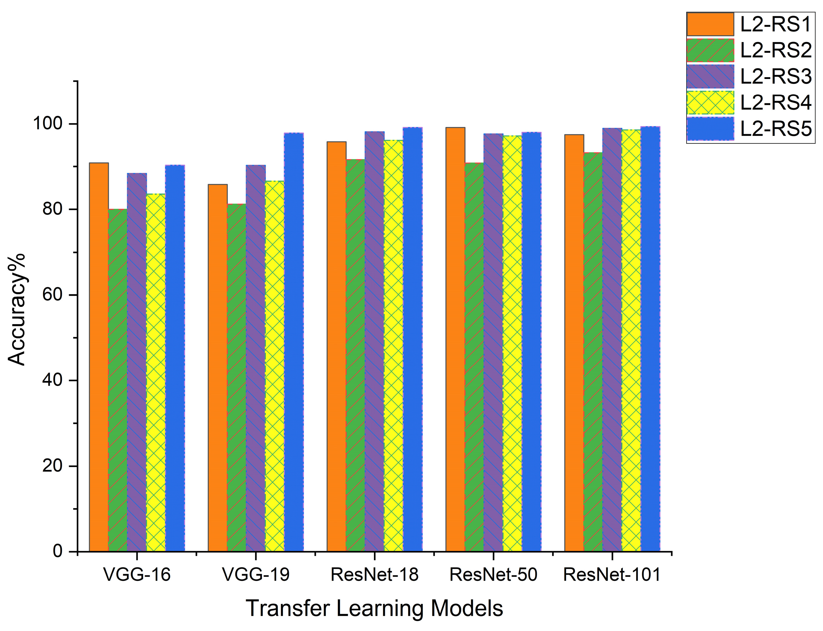
Table 10 displays the training accuracy for various transfer learning models in Case Study 3, where the load is 1000 N. Each model, including TL_VGG-16, TL_VGG-19, TL_ResNet-18, TL_ResNet-50, and TL_ResNet-101, is assessed over five runs (L1-RS1 through L1-RS5). The ResNet models exhibit exceptionally high accuracy, particularly TL_ResNet-18 and TL_ResNet-101, with the latter achieving the highest accuracy of 99.34% in L1-RS5. VGG models show more variability, with TL_VGG-19 reaching the highest accuracy in L1-RS5. These results suggest that while all models perform well, ResNet models, especially TL_ResNet-101, are highly effective for this diagnostic task under specified load conditions. The results of the training accuracy provided significant insights into the performance of various deep learning models in the diagnosis of bearing failure under a specific heavy load condition (1000 N). The data highlight the need to tailor the model selection according to load and rotational speed factors. The standout performances of TL_DenseNet-201 and TL_ResNet-101 suggest their potential as highly reliable and effective tools for bearing fault diagnosis in scenarios involving a 1000N load. The accuracy levels are high across all models, with ResNet-101 consistently showing the highest accuracy rates, followed closely by the other ResNet models. VGG-19 and VGG-16 also demonstrate high accuracy, but with slight variability across different runs. Figure 22 visualizes and compares each model’s reliability and performance in the context of the specific conditions of Case Study 3.

3.3. Testing Model on Unseen Data

3.3.1. Testing Model on Unseen Data from the Experiment

The multiclass confusion matrix presents a precise and unambiguous depiction of errors and their corresponding positions for each category in a multiclassification task. The vertical axis represents the actual labels, whereas the horizontal axis represents the predicted outcomes. The elements on the main diagonal represent the count of accurate judgment samples, whereas the remaining points indicate the number of incorrect judgments. Figure 23 shows the multiclass confusion matrix of TL_ResNet-101 when evaluating the model on unseen data from the experiment, specifically from L0-RS1 to L0-RS5.

The series of normalized confusion matrices reflects the classification performance of a machine learning model for bearing fault detection. We observed a high classification accuracy for most classes in these matrices, indicating a robust model. However, a closer examination revealed some areas of misclassification, suggesting opportunities for model improvement. For example, there is recurring confusion between classes, such as HB with IRF0.5, RF0.5, and ORF0.5, implying challenges in differentiating between healthy bearings and those with minor defects. Furthermore, as the severity of the defects increases, the model appears to struggle more to distinguish between different severity levels, which is evident in the confusion between IRF2 and IRF1 and between RF2 and RF1. L0-RS1 demonstrates exceptional precision, effectively eliminating misclassifications. L0-RS2 and L0-RS3 still show high accuracy with minor confusions between certain fault types, such as healthy bearing and inner race fault size 0.5. L0-RS4 continues the trend of high performance with slight confusion, primarily between outer race fault size 0.5 and inner race fault size 1. Finally, L0-RS5 indicates some misclassifications, notably with respect to the 0.5 fault size of the roller. These matrices highlight the high reliability and minor areas for improvement in fault diagnosis.

Table 11. Model performance across cases L0.

Case	Accuracy%	Measure	HB	IRF0.5	IRF1	IRF2	ORF0.5	ORF1	ORF2	RF0.5	RF1	RF2
L0-RS1	99.00	Precision	1.00	1.00	0.80	1.00	0.85	1.00	1.00	1.00	1.00	1.00
		Recall	1.00	0.77	1.00	1.00	0.94	1.00	1.00	1.00	1.00	1.00
		F1-Score	1.00	0.87	0.89	1.00	0.89	1.00	1.00	1.00	1.00	1.00
		Specificity	1.00	0.97	1.00	1.00	0.99	1.00	1.00	1.00	1.00	1.00
L0-RS2	97.38	Precision	1.00	0.95	0.79	1.00	1.00	1.00	1.00	1.00	1.00	1.00
		Recall	1.00	0.85	0.94	0.98	0.98	1.00	1.00	1.00	1.00	1.00
		F1-Score	1.00	0.90	0.86	0.99	0.99	1.00	1.00	1.00	1.00	1.00
		Specificity	1.00	0.98	0.99	1.00	1.00	1.00	1.00	1.00	1.00	1.00
L0-RS3	97.81	Precision	0.98	1.00	0.91	1.00	0.98	0.98	1.00	1.00	1.00	0.92
		Recall	1.00	0.96	0.98	0.98	1.00	1.00	1.00	1.00	0.88	1.00
		F1-Score	0.99	0.98	0.94	0.99	0.99	0.99	1.00	1.00	0.93	0.96
		Specificity	1.00	0.99	1.00	1.00	1.00	1.00	1.00	1.00	0.98	1.00
L0-RS4	98.57	Precision	1.00	0.96	0.94	1.00	0.99	0.99	0.99	1.00	1.00	0.99
		Recall	1.00	1.00	0.99	0.93	0.95	1.00	1.00	1.00	0.99	1.00
		F1-Score	1.00	0.98	0.96	0.97	0.97	0.99	0.99	1.00	0.99	0.99
		Specificity	1.00	1.00	1.00	0.99	0.99	1.00	1.00	1.00	1.00	1.00
L0-RS5	98.77	Precision	1.00	1.00	0.98	0.98	0.99	1.00	1.00	0.95	0.97	1.00
		Recall	0.95	0.96	1.00	1.00	0.97	0.99	1.00	1.00	1.00	1.00
		F1-Score	0.98	0.98	0.99	0.99	0.98	1.00	1.00	0.98	0.99	1.00
		Specificity	0.99	1.00	1.00	1.00	1.00	1.00	1.00	1.00	1.00	1.00

presents the performance metrics of a diagnostic model for rolling element bearings in five test cases (L0-RS1 to L0-RS5). It includes precision, recall, specificity, F1 score, and accuracy for different bearing conditions. Precision measures the proportion of true positives against all positive predictions, indicating the accuracy when it predicts a fault. Recall, or sensitivity, assesses the model’s ability to identify actual faults correctly. The F1 score is a balanced measure of precision and recall, useful for uneven class distributions. Specificity measures the model’s ability to correctly identify true negatives, which is crucial for avoiding false alarms. Together, these metrics provide a comprehensive understanding of diagnostic accuracy. Starting with the L0-RS1 case, the model achieves an exceptional 99% overall accuracy, demonstrating perfect precision, recall, F1 score, and specificity across all classes. This indicates an extraordinary ability to accurately diagnose faults, identify healthy bearings without errors, and minimize false positives and negatives. However, a change is observed in the L0-RS2 case, where the accuracy slightly drops to 97.38%. Here, the precision and recall for classes like IRF0.5 and IRF1 show minor declines, hinting at challenges in accurately identifying smaller inner race faults. Despite this, the high specificity across all classes maintains the model’s credibility in avoiding false positives.

The trend of slight performance fluctuation continues in L0-RS3, with an overall accuracy of 97.81%. The model experiences a marginal decrease in precision for IRF0.5 and RF2 and in recall for IRF1 and RF1, which could indicate a somewhat reduced ability to detect these specific fault types. However, the consistently high specificity underscores the model’s strength to effectively rule out false positives. In L0-RS4, the overall precision reaches 98.57%, with a noticeable decrease in recall for IRF2 and a slight decrease in precision for IRF1. These changes suggest some difficulty in accurately identifying these faults, yet the high specificity across all classes reassures us of the model’s effectiveness in correctly identifying true negatives.

Finally, L0-RS5 shows an overall accuracy of 98.77%, where precision, recall, and F1 scores remain high for most classes. However, slight decreases in precision and recall are observed for IRF0.5 and RF1. Again, the model maintains a consistently high specificity, effectively ruling out non-fault conditions.

In summary, the model exhibits robust performance across various types and sizes, with exceptional accuracy in some cases, such as L0-RS1. However, it also presents areas for potential refinement, particularly in identifying specific fault types under different operating conditions. The consistently high specificity across all cases is a testament to the model’s ability to correctly identify true negatives, a crucial feature in practical applications to avoid unnecessary maintenance actions based on false positives. Variations in precision and recall across the cases underscore the importance of ongoing optimization, especially for fault types where these metrics are less than ideal.

Table A1. Model performance across cases L1.

Case	Accuracy%	Measure	HB	IRF0.5	IRF1	IRF2	ORF0.5	ORF1	ORF2	RF0.5	RF1	RF2
L1-RS1	91.50	Precision	1.00	0.75	1.00	0.95	0.95	1.00	1.00	0.95	0.85	0.70
		Recall	0.95	1.00	0.87	0.90	1.00	1.00	1.00	0.83	0.71	1.00
		F1-Score	0.98	0.86	0.93	0.93	0.97	1.00	1.00	0.88	0.77	0.82
		Specificity	0.99	1.00	0.98	0.99	1.00	1.00	1.00	0.98	0.96	1.00
L1-RS2	95.48	Precision	1.00	0.69	0.98	0.95	1.00	1.00	1.00	0.98	0.98	0.98
		Recall	1.00	0.94	1.00	0.74	1.00	1.00	1.00	0.93	1.00	1.00
		F1-Score	1.00	0.79	0.99	0.83	1.00	1.00	1.00	0.95	0.99	0.99
		Specificity	1.00	0.99	1.00	0.96	1.00	1.00	1.00	0.99	1.00	1.00
L1-RS3	90.78	Precision	1.00	0.53	0.95	0.95	1.00	0.98	0.97	0.77	1.00	0.92
		Recall	0.85	0.97	0.67	1.00	1.00	0.97	1.00	1.00	0.81	1.00
		F1-Score	0.92	0.69	0.79	0.98	1.00	0.98	0.98	0.87	0.90	0.96
		Specificity	0.98	1.00	0.95	1.00	1.00	1.00	1.00	1.00	0.97	1.00
L1-RS4	91.79	Precision	0.32	0.96	1.00	1.00	0.99	1.00	1.00	1.00	0.90	1.00
		Recall	1.00	1.00	1.00	0.99	1.00	1.00	1.00	0.95	1.00	0.57
		F1-Score	0.49	0.98	1.00	0.99	0.99	1.00	1.00	0.98	0.95	0.72
		Specificity	1.00	1.00	1.00	1.00	1.00	1.00	1.00	0.99	1.00	0.92
L1-RS5	92.62	Precision	0.62	0.98	1.00	0.77	1.00	1.00	1.00	0.96	0.93	1.00
		Recall	0.90	0.93	0.86	0.72	0.99	1.00	0.99	0.95	1.00	0.94
		F1-Score	0.73	0.95	0.92	0.75	0.99	1.00	0.99	0.96	0.96	0.97
		Specificity	0.99	0.99	0.98	0.97	1.00	1.00	1.00	0.99	1.00	0.99

in Appendix B.1 evaluates the performance of a diagnostic model for Case Study 2 (L1), where various runs (L1-RS1 to L1-RS5) are analyzed for different classes of bearing faults at a load of 500 N. The accuracy, precision, recall, F1 score, and specificity are provided for each type of fault. Precision indicates how often the model’s predictions for a specific fault type were correct, recall measures the model’s ability to identify all actual instances of a fault type, F1-score gives a balance between precision and recall, and specificity indicates the model’s ability to identify true negatives for each fault type correctly. Together, these metrics provide a holistic view of the model’s diagnostic capabilities for Case Study 2 under this specific load condition. The confusion matrices are shown in Appendix B.2 for the five runs of Case Study 2. The ResNet-101 model exhibits varying levels of diagnostic accuracy. In the first run, L1-RS1, the model generally achieves high accuracy; however, distinguishing between roller fault sizes 1 (RF1) and 2 (RF2) is difficult. The second run, L1-RS2, uncovers challenges in differentiating between inner race fault sizes 1 (IRF1) and 2 (IRF2), as well as between the slightest roller fault (RF0.5) and size 1 (RF1).

During the third run, L1-RS3, the model’s performance is strong, yet it exhibits occasional confusion between outer race fault size 0.5 (ORF0.5) and size 2 (ORF2), and between roller faults RF0.5 and RF1. In the fourth run, L1-RS4, issues arise with the model mistaking healthy bearings (HBs) for inner race fault size 0.5 (IRF0.5) and confusing RF1 with RF2. Lastly, the fifth run, L1-RS5, presents significant misclassifications, notably confusing healthy bearings with more minor inner race faults and consistently struggling to distinguish between the two sizes of roller faults (RF1 and RF2).

Table A2. Model performance across cases for Case Study 3 (L2).

Case	Accuracy%	Measure	HB	IRF0.5	IRF1	IRF2	ORF0.5	ORF1	ORF2	RF0.5	RF1	RF2
L2-RS1	98.50	Precision	1.00	1.00	1.00	1.00	1.00	1.00	1.00	1.00	0.90	0.95
		Recall	0.95	0.95	1.00	1.00	1.00	1.00	1.00	1.00	0.95	1.00
		F1-Score	0.98	0.98	1.00	1.00	1.00	1.00	1.00	1.00	0.92	0.97
		Specificity	0.99	0.99	1.00	1.00	1.00	1.00	1.00	1.00	0.99	1.00
L2-RS2	97.38	Precision	1.00	1.00	0.55	0.90	0.98	0.93	0.74	1.00	0.95	1.00
		Recall	0.98	0.93	1.00	1.00	1.00	0.78	1.00	0.91	0.68	0.95
		F1-Score	0.99	0.97	0.71	0.95	0.99	0.85	0.85	0.95	0.79	0.98
		Specificity	1.00	0.99	1.00	1.00	1.00	0.97	1.00	0.99	0.95	0.99
L2-RS3	98.83	Precision	1.00	1.00	1.00	0.99	1.00	0.93	0.98	1.00	1.00	1.00
		Recall	1.00	1.00	1.00	1.00	1.00	0.99	0.84	0.98	1.00	1.00
		F1-Score	1.00	1.00	1.00	1.00	1.00	0.96	0.91	0.99	1.00	1.00
		Specificity	1.00	1.00	1.00	1.00	1.00	1.00	0.99	1.00	1.00	1.00
L2-RS4	96.43	Precision	1.00	0.80	1.00	1.00	1.00	1.00	0.95	0.98	0.92	1.00
		Recall	1.00	0.97	1.00	1.00	1.00	1.00	1.00	0.83	1.00	0.88
		F1-Score	1.00	0.88	1.00	1.00	1.00	1.00	0.98	0.90	0.96	0.94
		Specificity	1.00	1.00	1.00	1.00	1.00	1.00	1.00	0.98	1.00	0.99
L2-RS5	94.64	Precision	0.99	1.00	0.82	0.99	1.00	1.00	1.00	0.74	0.94	0.99
		Recall	1.00	0.72	1.00	0.94	1.00	0.98	1.00	1.00	0.99	0.94
		F1-Score	0.99	0.84	0.90	0.97	1.00	0.99	1.00	0.85	0.96	0.97
		Specificity	1.00	0.96	1.00	0.99	1.00	1.00	1.00	1.00	1.00	0.99

details the performance metrics of a diagnostic model tested in Case Study 3 (L2), captured over five runs (L2-RS1 through L2-RS5). Efficacy is measured using precision, recall, F1 score, and specificity for various classes of bearing faults, namely healthy bearing (HB), inner race fault (IRF) sizes 0.5, 1, and 2, outer race fault (ORF) sizes 0.5, 1, and 2, and roller fault (RF) sizes 0.5, 1, and 2. For L2-RS1, the model boasts an overall precision of 98.50% with perfect precision across most fault types, although it slightly falters in precision and recall for RF1 and RF2. The F1 scores, except for RF1, are correspondingly high, indicating a generally balanced precision–recall relationship. The specificity is near perfect, suggesting an excellent true negative identification. In L2-RS2, there is a marginal decrease in accuracy to 97.38%. Here, the precision for IRF1 and ORF1 drops markedly, and recall also decreases for RF0.5 and RF1. This run exhibits a dip in performance, particularly in the balanced F1 score for IRF1, indicating room for improvement in the model’s classification of these fault types. L2-RS3 sees a slight increase in overall accuracy at 98.83%. Precision maintains a high standard across all classes, with a minor decrease for RF1 and RF2. Recall and F1 scores remain consistently high, but there is a noticeable drop in ORF2 recall. Specificity remains high, reinforcing the model’s reliability in ruling out non-fault conditions. For L2-RS4, the accuracy drops slightly to 96.43%. There is a decrease in precision for IRF0.5 and a significant reduction in recall for RF0.5, with corresponding effects on the F1 score, reflecting the need for better identification of these fault types. Despite this, the specificity is still strong. Finally, L2-RS5 shows an overall precision of 94.64%, with the lowest precision for RF0.5 and the lowest recall for IRF0.5, RF1, and RF2 among the runs. The F1 score and specificity also take a hit, suggesting that this run’s model performance is the weakest, particularly in distinguishing between these fault types.

The confusion matrices shown in Appendix C.2 represent the classification test results for Case Study 2 over five runs (L2-RS1 through L2-RS5). In L2-RS1, the matrix suggests excellent model performance with perfect classification for most classes, except for a slight confusion between RF1 and RF2. The L2-RS2 matrix reveals more variability with noticeable misclassifications, such as between IRF1 and other fault types, suggesting difficulty distinguishing between specific inner race fault sizes. In L2-RS3, the model appears to have high accuracy again with minor confusion, such as slightly misclassifying ORF0.5 as ORF2.

The L2-RS4 matrix shows a high degree of precision, but with some misclassification between RF0.5 and other fault types, indicating specific areas where the model could improve.

Lastly, L2-RS5 shows excellent overall performance, with minor confusion between IRF1 and IRF2, and between RF1 and other faults, pointing to potential difficulties in distinguishing similar fault conditions.

3.3.2. Testing the Model on Unseen Data for IMS

To evaluate the efficacy of the proposed technique using the IMS dataset, the data were initially transformed into images using Scattergram Filter Bank 1. Subsequently, the MATLAB script provided in Appendix B was used to test the TL_ResNet-101 model. The model, saved as ‘TL_Model.mat’ following the training phase, was then ready for use in the testing phase.

The TL_ResNet-101 model can classify new images. This process involves loading a new image, modifying its size to match the input criteria of the model, and then applying the model to determine its category. The MATLAB code for prediction is illustrated in Appendix D. This code iterates through each image in the specified folder, resizes it, classifies it using the TL_ResNet-101 model, and stores the filename, predicted class, and classification confidence in a table. After the script, the results were reviewed using MATLAB. The highest predictions of the segment scores are presented in

Table 12. Test results of Set No.1 from the IMS dataset.

Experiment			L0-RS4		L1-RS4		L2-RS4
Fault Position	Sensor Channel	Direction of Measurement	Predicted Label	Accuracy	Predicted Label	Accuracy	Predicted Label	Accuracy
B3	CHX	Vertical	RF1	62.54	IRF2	98.05	“RF0.5”	99.964
B3	CHY	Horizontal	RF0.5	96.82	IRF2	97.85	“RF0.5”	99.656
B4	CHX	Vertical	“RF0.5”	0.99957	RF2	76.53	“RF0.5”	99.852
B4	CHY	Horizontal	“RF1”	0.99823	RF2	99.94	RF0.5	96.784

.

The model demonstrates high predictive accuracy in most cases, particularly in the L2-RS4 scenario in all fault positions and directions. This indicates its robustness and effectiveness in diagnosing bearing faults in various load and speed conditions. Variable accuracy levels, particularly in the L0-RS4 and L1-RS4 scenarios, suggest that the fault’s specific operational conditions or characteristics may influence the model’s performance. The moderate accuracy in some cases (L0-RS4 for B3-CHX) indicates potential areas for model refinement.

Table 13. Testing in Set No.2 of the IMS dataset.

Experiment			L0-RS4		L1-RS4		L2-RS4
Fault Position	Sensor Channel	Direction of Measurement	Predicted Label	Accuracy%	Accuracy%	Predicted Label	Predicted Label	Accuracy%
B1	CHX	Vertical	ORF2”	99.979	99.99	ORF2	RF0.5	96.028

presents the results using transfer learning with TL_ResNet-101 to predict the type of fault in Set No.2 of the IMS data set. The model achieved exceptionally high accuracy (99.979% and 99.99%) in predicting the type of fault labeled ORF2 for the early fault (L0-RS4 and L1-RS4, respectively). This indicates that ResNet-101, when combined with transfer learning, is highly effective for early fault detection, which is a critical aspect of preventive maintenance.

For the advanced fault stage (L2-RS4), the accuracy dropped to 96.028%, with the predicted label changing to RF0.5. This decrease in accuracy can be attributed to the increased complexity of the fault characteristics at this stage. This suggests that although the model is robust in early detection, its performance varies with the progression of fault severity.

Table 14. Testing in Set No.3 of the IMS dataset.

Experiment			L0-RS4		L1-RS4		L2-RS4
Fault Position	Sensor Channel	Direction of Measurement	Predicted Label	Accuracy %	Predicted Label	Accuracy %	Predicted Label	Accuracy
B3	CHX	Vertical	ORF2	99.871	ORF2	99.949	“RF2”	97.927

presents the test results on Set No.3 of the IMS dataset, focusing on bearing 3 (B3) across three levels of fault severity (L0-RS4, L1-RS4, and L2-RS4). The experiment utilized transfer learning on TL_ResNet-101 to analyze data from the CHX sensor channel in the vertical direction. The model achieved high precision in the early (L0-RS4) and intermediate (L1-RS4) fault stages with scores of 99.871% and 99.949%, respectively. Both stages were predicted as ORF2. This high accuracy indicates the robustness of the model in detecting early- to mid-stage faults, which is crucial for timely maintenance interventions.

3.4. Comparison of this Work with Previous Research

Table 15. Comparison of previous research with this work.

Researcher(s)	Type of Model	Operating Speed Range	Accuracy
[36]	Knowledge Addition-Based Transfer Learning	2050	93%
[47]	Deep Transfer Learning and Adaptive Weighting CNN-LSTM	750–1500 RPM	71.8%
[48]	Deep Transfer Learning Strategy for Efficient Domain Generalization in Machine Fault Diagnosis	1000–1400 RPM	96.89%
[49]	CNN and Transfer Learning with Empirical Mode Decomposition Pseudo-Wigner–Ville Distribution (EP)8	Various	96.67%
[50]	L-CNN	800–1200 RPM	95.4%
Current work	Deep Transfer Learning with ResNet-101, VGG-16, VGG19, ResNet-18, and ResNet-50	500–2500 RPM	90.78–99%

shows a range of models, from knowledge addition-based transfer learning, seen in Kumar et al. (2023) [36], to more complex frameworks such as deep transfer learning with ResNet-101, VGG-16, VGG19, ResNet-18, and ResNet-50, used in the current work. This diversity indicates that a broad spectrum of methodologies is being explored in the field, each with unique strengths. The accuracies achieved in these studies were impressive, with current work reaching up to 99%. This high level of precision, especially compared to earlier works such as [36] which demonstrated a 93% precision rate, indicates continuous improvements in fault diagnosis techniques, and the use of advanced deep transfer learning models in the current work could contribute to this high accuracy. Some studies, such as those of Li et al. [40], integrated CNN with the pseudo-Wigner–Ville empirical mode decomposition distribution, highlighting innovative combinations of techniques to improve diagnostic capabilities. Similarly, integrating multiple advanced architectures, such as ResNet-101, VGG-16, VGG19, ResNet-18, and ResNet-50, in the current work, demonstrates a trend toward complex, multifaceted approaches. The variable operating speed ranges and high accuracy indicate the potential of these models for real-world applications. As in the current study, models that operate effectively across a wide range of speeds are important for diverse industrial settings. The evolution from simpler models to more complex and accurate systems indicates a trend towards integrating multiple deep learning techniques.

4. Conclusions

This study aims to fill the gap in spherical bearing fault diagnosis methods by presenting an innovative approach that combines advanced machine learning techniques with practical application considerations. This study successfully demonstrated the efficacy of using transfer learning, specifically the ResNet-101 model, in the fault diagnosis of spherical roller bearings under varying operating conditions. The key findings of this study indicate that transfer learning can significantly improve the accuracy and efficiency of fault diagnosis in mechanical bearings, which is a critical component in numerous industrial applications. Experiments conducted with SKF 2209EK spherical roller bearings yield promising results, showing the model’s ability to identify and diagnose faults accurately. This performance is particularly notable given the challenges of varying operating conditions and the need for robust diagnostic tools in dynamic industrial environments.

The findings of this study underscore the potential of advanced machine learning techniques, specifically transfer learning coupled with ResNet-101, in the field of mechanical fault diagnosis. The high precision of the model can be attributed to the effective signal-to-image transformation using Scattergram Filter Bank 1, which allows for a detailed representation of vibration signals. This approach addresses the challenge of limited labeled data and improves diagnostic accuracy under varying operational conditions. Furthermore, the adoption of a multidirectional vibration data analysis provides a more nuanced understanding of bearing conditions, surpassing the limitations of traditional single-direction analysis. The methodology and results could serve as a benchmark for future research in this domain, especially in spherical bearings, to address the challenge of limited labeled data and improve diagnostic accuracy under varying operational conditions. Additionally, the adoption of a multidirectional vibration data analysis provides a more nuanced understanding of bearing conditions, surpassing the limitations of traditional single-direction analysis.

In conclusion, this study presents a significant step forward in applying advanced machine learning techniques for mechanical fault diagnosis. It offers a foundation upon which future research can be built, with the aim to further expand the capabilities of such technologies in industrial maintenance.

References

1. Zhao, H.; Yang, X.; Chen, B.; Chen, H.; Deng, W. Bearing fault diagnosis using transfer learning and optimised deep belief network. Meas. Sci. Technol. 2022, 33, 065009. [Google Scholar] [CrossRef]
2. Ma, P.; Zhang, H.; Fan, W.; Wang, C. A diagnosis framework based on domain adaptation for bearing fault diagnosis across diverse domains. ISA Trans. 2020, 99, 465–478. [Google Scholar] [CrossRef] [PubMed]
3. Manikandan, M.; Duraivelu, K. Machine learning algorithms for industrial fault diagnosis: Challenges and solutions. Mech. Syst. Signal Process. 2021, 144, 106932. [Google Scholar]
4. Guo, L.; Lei, Y.; Xing, S.; Yan, T.; Li, N. Deep convolutional transfer learning network: A new method for intelligent fault diagnosis of machines with unlabeled data. IEEE Trans. Ind. Electron. 2018, 66, 7316–7325. [Google Scholar] [CrossRef]
5. Gousseau, W.; Antoni, J.; Girardin, F.; Griffaton, J. Analysis of the Rolling Element Bearing data set of the Center for Intelligent Maintenance Systems of the University of Cincinnati. In Proceedings of the CM2016, Paris, France, 10–12 October 2016. [Google Scholar]
6. Huang, H.; Baddour, N. Bearing vibration data collected under time-varying rotational speed conditions. Data Brief 2018, 21, 1745–1749. [Google Scholar] [CrossRef] [PubMed]
7. Wang, B.; Lei, Y.; Li, N.; Li, N. A hybrid prognostics approach for estimating remaining useful life of rolling element bearings. IEEE Trans. Reliab. 2020, 69, 401–412. [Google Scholar] [CrossRef]
8. Deng, J.; Dong, W.; Socher, R.; Li, L.; Li, K.; Li, F. ImageNet: A large-scale hierarchical image database. In Proceedings of the IEEE Conference on Computer Vision and Pattern Recognition, Miami, FL, USA, 20–25 June 2009. [Google Scholar]
9. Weiss, K.; Khoshgoftaar, T.M.; Wang, D. A survey of transfer learning. J. Big Data 2016, 3, 9. [Google Scholar] [CrossRef]
10. Singh, A.; Moore, K.J. Identification of multiple local nonlinear attachments using a single measurement case. J. Sound Vib. 2021, 506, 116410. [Google Scholar] [CrossRef]
11. Singh, A.; Moore, K.J. Characteristic nonlinear system identification of local attachments with clearance nonlinearities. Nonlinear Dyn. 2020, 102, 1667–1684. [Google Scholar] [CrossRef]
12. Li, X.; Zhang, W.; Ma, H.; Luo, Z.; Li, X. Deep learning-based adversarial multi-classifier optimization for cross-domain machinery fault diagnostics. J. Manuf. Syst. 2020, 55, 334–347. [Google Scholar] [CrossRef]
13. Zhang, M.; Wang, D.; Lu, W.; Yang, J.; Li, Z.; Liang, B. A deep transfer model with wasserstein distance guided multi-adversarial networks for bearing fault diagnosis under different working conditions. IEEE Access 2019, 7, 65303–65318. [Google Scholar] [CrossRef]
14. Zhang, R.; Gu, Y. A Transfer Learning Framework with a One-Dimensional Deep Subdomain Adaptation Network for Bearing Fault Diagnosis under Different Working Conditions. Sensors 2022, 22, 1624. [Google Scholar] [CrossRef] [PubMed]
15. Chen, J.; Li, J.; Huang, R.; Yue, K.; Chen, Z.; Li, W. Federated Transfer Learning for Bearing Fault Diagnosis with Discrepancy-Based Weighted Federated Averaging. IEEE Trans. Instrum. Meas. 2022, 71, 3514911. [Google Scholar] [CrossRef]
16. Bhuiyan, M.R.; Uddin, J. Deep Transfer Learning Models for Industrial Fault Diagnosis Using Vibration and Acoustic Sensors Data: A Review. Vibration 2023, 6, 218–238. [Google Scholar] [CrossRef]
17. Han, T.; Xie, W.; Pei, Z. Semi-supervised adversarial discriminative learning approach for intelligent fault diagnosis of wind turbine. Inf. Sci. 2023, 648, 119496. [Google Scholar] [CrossRef]
18. Kaya, Y.; Kuncan, F.; Ertunç, H.M. A new automatic bearing fault size diagnosis using time-frequency images of CWT and deep transfer learning methods. Turk. J. Electr. Eng. Comput. Sci. 2022, 30, 1851–1867. [Google Scholar] [CrossRef]
19. Singh, A.; Singh, S. A systematic review of rolling bearing fault diagnoses based on deep learning techniques. J. Fail. Anal. Prev. 2023. [Google Scholar] [CrossRef]
20. Zhang, L.; Zhou, D. A survey of machine learning techniques for condition monitoring and fault diagnosis. Appl. Sci. 2021, 11, 1904. [Google Scholar] [CrossRef]
21. Li, X.; Zhang, W. Enhancing bearing fault diagnosis using transfer learning and random forest classification: A comparative study on variable working conditions. Mech. Syst. Signal Process. 2022. [Google Scholar] [CrossRef]
22. Nectoux, P.; Gouriveau, R.; Medjaher, K.; Ramasso, E.; Chebel-Morello, B.; Zerhouni, N.; Varnier, C. PRONOSTIA: An experimental platform for bearings accelerated degradation tests. In Proceedings of the IEEE International Conference on Prognostics and Health Management, PHM’12, Minneapolis, MN, USA, 23–27 September 2012. [Google Scholar]
23. Lei, Y.; Yang, B.; Jiang, X.; Jia, F.; Li, N.; Nandi, A.K. Applications of machine learning to machine fault diagnosis: A review and roadmap. Mech. Syst. Signal Process. 2020, 138, 106587. [Google Scholar] [CrossRef]
24. Zhang, Y.; Wang, Y.; Li, X. Deep learning for fault diagnosis and prognosis: Current status and future challenges. Measurement 2021, 173, 108561. [Google Scholar]
25. Mushtaq, N.; Reddy, M. Intelligent fault diagnosis of rotating machinery with convolutional neural networks. J. Sound Vib. 2021, 491, 115735. [Google Scholar]
26. Hamadache, M.; Kechida, S.; Srairi, K. Deep learning algorithms and hardware implementations: A survey. Microprocess. Microsyst. 2019, 103, 104023. [Google Scholar]
27. Lei, Y.; Li, N.; Gontarz, S.; Lin, J.; Radkowski, S.; Dybała, J. A review on empirical mode decomposition in fault diagnosis of rotating machinery. Mech. Syst. Signal Process. 2016, 35, 108–126. [Google Scholar] [CrossRef]
28. Zabin, M.; Choi, H.-J.; Uddin, J. Hybrid deep transfer learning architecture for industrial fault diagnosis using Hilbert transform and DCNN–LSTM. J. Supercomput. 2022, 78, 10377–10394. [Google Scholar] [CrossRef]
29. Zhang, Y.; Wang, Y. A review of recent advances in wind turbine condition monitoring and fault diagnosis. Power Syst. 2020, 25, 1753–1766. [Google Scholar]
30. Mushtaq, N.; Reddy, M. Role of big data analytics in industrial fault diagnostics: A review. Mech. Syst. Signal Process. 2021, 151, 107398. [Google Scholar]
31. Hakim, D.; Singh, R. Transfer learning in machinery fault diagnosis: A systematic review. Reliab. Eng. Syst. Saf. 2022, 206, 107312. [Google Scholar]
32. Wang, J.; Zhao, M. Machine learning-based bearing fault diagnosis: Review of the Case Western Reserve University data. IEEE Access 2022. [Google Scholar]
33. Zhao, L.; Wang, X.; Li, Y.; Chen, M.; Zhang, T.; Liu, Q.; Yang, H.; Sun, J.; Guo, P.; Hu, R.; et al. Recent advances in the application of deep learning for fault diagnosis. Mech. Syst. Signal Process. 2022. [Google Scholar]
34. Zhao, R.; Yan, R.; Wang, J.; Mao, K. Fault Diagnosis of Rotating Machinery with Double Row Spherical Roller Bearings Using Advanced Vibration Analysis Techniques. J. Phys. Conf. Ser. 2022. [Google Scholar]
35. Lee, J.; Qiu, H.; Yu, G.; Lin, J.; Rexnorf Technical Services IMS, University of Cincinnati. Bearing Data Set; NASA Prognostics Data Repository, NASA Ames Research Center: Moffett Field, CA, USA, 2007. [Google Scholar]
36. Kumar, A.; Glowacz, A.; Tang, H.; Xiang, J. Knowledge addition for improving the transfer learning from the laboratory to identify defects of hydraulic machinery. Eng. Appl. Artif. Intell. 2023, 126, 106756. [Google Scholar] [CrossRef]
37. Li, X.; Zhang, C.; Li, X.; Zhang, W. Federated transfer learning in fault diagnosis under data privacy with target self-adaptation. J. Manuf. Syst. 2023, 68, 523–535. [Google Scholar] [CrossRef]
38. Liang, M.; Zhou, K. A hierarchical deep learning framework for combined rolling bearing fault localisation and identification with data fusion. J. Vib. Control 2022, 29, 3165–3174. [Google Scholar] [CrossRef]
39. Guo, Y.; Zhang, J.; Sun, B.; Wang, Y. Adversarial Deep Transfer Learning in Fault Diagnosis: Progress, Challenges, and prospects. Sensors 2023, 23, 7263. [Google Scholar] [CrossRef] [PubMed]
40. Li, J.; Liu, Y.; Li, Q. Generative adversarial network and transfer-learning-based fault detection for rotating machinery with imbalanced data condition. Meas. Sci. Technol. 2021, 33, 045103. [Google Scholar] [CrossRef]
41. Qian, Y.; Yan, R.; Gao, R.X.; Chen, X. Deep Transfer Learning for Intelligent Fault Diagnosis of Machinery: A Comprehensive Review. Neural Process. Lett. 2022. [Google Scholar] [CrossRef]
42. Wang, Y.; He, Z.; Zi, Y. A New Approach to Intelligent Fault Diagnosis of Rotating Machinery with Dual-Channel Data. IEEE Trans. Ind. Electron. 2022. [Google Scholar] [CrossRef]
43. SKF. Spherical Roller Bearing 22209 EK. Available online: https://www.skf.com/in/products/rolling-bearings/roller-bearings/spherical-roller-bearings/productid-22209%20EK (accessed on 1 January 2024).
44. SKF Group. Bearing Damage and Failure Analysis. [PDF File]. Available online: https://cdn.skfmediahub.skf.com/api/public/0901d1968064c148/pdf_preview_medium/0901d1968064c148_pdf_preview_medium.pdf (accessed on 1 January 2024).
45. Tu, W.; Yang, J.; Luo, Y.; Jiang, L.; Xu, J.; Yu, W. Vibration transmission characteristics and measuring points analysis of bearing housing system. Shock Vib. 2022, 2022, 4334398. [Google Scholar] [CrossRef]
46. MathWorks. Wavelet Scattering—MATLAB & Simulink. 2023. Available online: https://www.mathworks.com/help/wavelet/ref/waveletscattering.scattergram.html (accessed on 1 January 2024).
47. Liu, Y.; Fan, K. Roller Bearing Fault Diagnosis Using Deep Transfer Learning and Adaptive Weighting. J. Phys. Conf. Ser. 2023, 2467, 012011. [Google Scholar] [CrossRef]
48. Asutkar, S.; Tallur, S. Deep transfer learning strategy for efficient domain generalisation in machine fault diagnosis. Nat. Commun. 2022, 13, 6607. [Google Scholar] [CrossRef] [PubMed]
49. Li, Y.; Zhang, H.; Li, Z. CNN and transfer learning with empirical mode decomposition-pseudo-Wigner–Ville distribution for bearing fault diagnosis. Mech. Syst. Signal Process. 2021, 167, 107401. [Google Scholar]
50. Changchang, A.; Li, B.; Wang, C. L-CNN for high-speed spindle fault detection. J. Manuf. Syst. 2019, 52, 125–138. [Google Scholar]
Figure 1. Schematic diagram of the experimental test rig.
Vibration 07 00028 g001
Figure 2. (a) Spherical roller bearing 22209 EK, and (b) dimensions [43].
Vibration 07 00028 g002
Figure 3. Common rolling element faults [44].
Vibration 07 00028 g003
Figure 4. Creating defective components of experimental work using an EDM: (a) inner race, (b) outer race, and (c) roller.
Vibration 07 00028 g004
Figure 5. Inner race defects: (a) inner race defect 0.5 mm, (b) inner race defect 1 mm, and (c) inner race defect 2 mm.
Vibration 07 00028 g005
Figure 6. Outer race defects: (a) outer race defect 0.5 mm, (b) outer race defect 1 mm, and (c) outer race defect 2 mm.
Vibration 07 00028 g006
Figure 7. Roller race defects: (a) roller defect 0.5 mm, (b) roller defect 1 mm, and (c) roller defect 2 mm.
Vibration 07 00028 g007
Figure 8. The alignment procedure using the Fixturlaser XA system.
Vibration 07 00028 g008
Figure 9. Hydraulic load system.
Vibration 07 00028 g009
Figure 10. Data acquisition and power control.
Vibration 07 00028 g010
Figure 11. SKF optical tachometer TMOT6.
Vibration 07 00028 g011
Figure 12. The measurement of vibrations using the SKF Microlog loading case.
Vibration 07 00028 g012
Figure 13. CMSS 2200 accelerometer sensor with magnetic base.
Vibration 07 00028 g013
Figure 14. Schematic diagram of the experimental procedure.
Vibration 07 00028 g014
Figure 15. The vibration measurements within the unloading case.
Vibration 07 00028 g015
Figure 16. (a) Segmentation of the signal, and (b) Scalogram filter bank 1 for each bearing condition.
Vibration 07 00028 g016aVibration 07 00028 g016bVibration 07 00028 g016c
Figure 17. (a) IMS bearing test rig, (b) Rexnord ZA-2115 double row bearing, (c) inner race defect in bearing 3, test 1, (d) roller element defect in bearing 4, test 1, and (e) outer race defect in bearing 1, test 2 [35].
Vibration 07 00028 g017
Figure 18. Raw vibration data for L0-RS1 in vertical and horizontal directions.
Vibration 07 00028 g018aVibration 07 00028 g018bVibration 07 00028 g018c
Figure 19. Confusion matrix chart of fault diagnosis results for TL_ ResNet-101 obtained for Case Study 1 (L0). (a) L0-RS1, (b) L0-RS2, (c) L0-RS3, (d) L0-RS4, and (e) L0-RS5.
Vibration 07 00028 g019aVibration 07 00028 g019b
Figure 20. Transfer learning model accuracy for Case Study 1.
Vibration 07 00028 g020
Figure 21. Training accuracy for Case Study 2.
Vibration 07 00028 g021
Figure 22. Training accuracy for Case Study 3.
Vibration 07 00028 g022
Figure 23. Confusion matrix of ResNet-101: (a) L0-RS1, (b) L0-RS2, (c) L0-RS3, (d) L0-RS4, and (e) L0-RS5.
Vibration 07 00028 g023