


Optimal Placement and Active Control Methods for Integrating Smart Material in Dynamic Suppression Structures

 ,
,  ,
,
Abstract
:1. Introduction
- -
- Modeling of intelligent constructs execution of control in oscillation suppression.
- -
- Uncertainties in dynamic loading.
- -
- Measurement noise.
- -
- Appropriate selection of weights for complete suppression of oscillations.
- -
- Using various choice places to stifle oscillations.
- -
- Results in the frequency domain as well as the time-space domain.
- -
- Introduction of the uncertainties in the construction’s mathematical model.
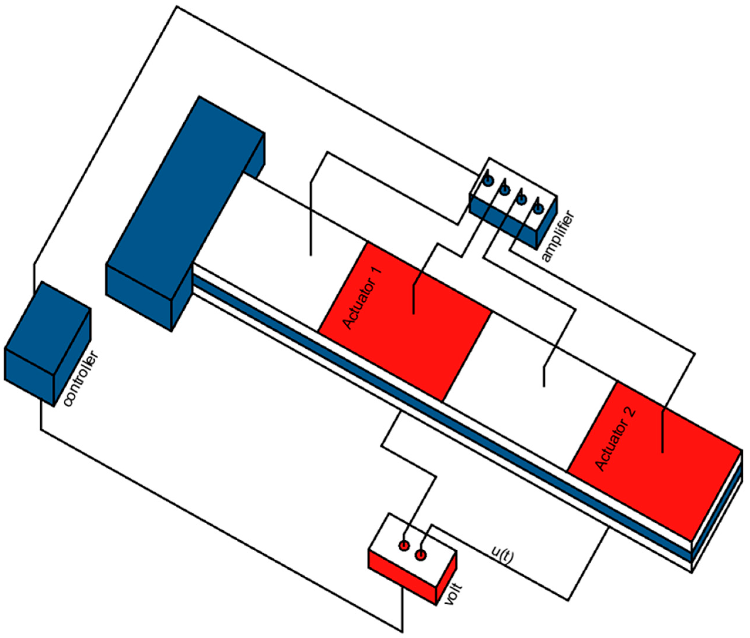
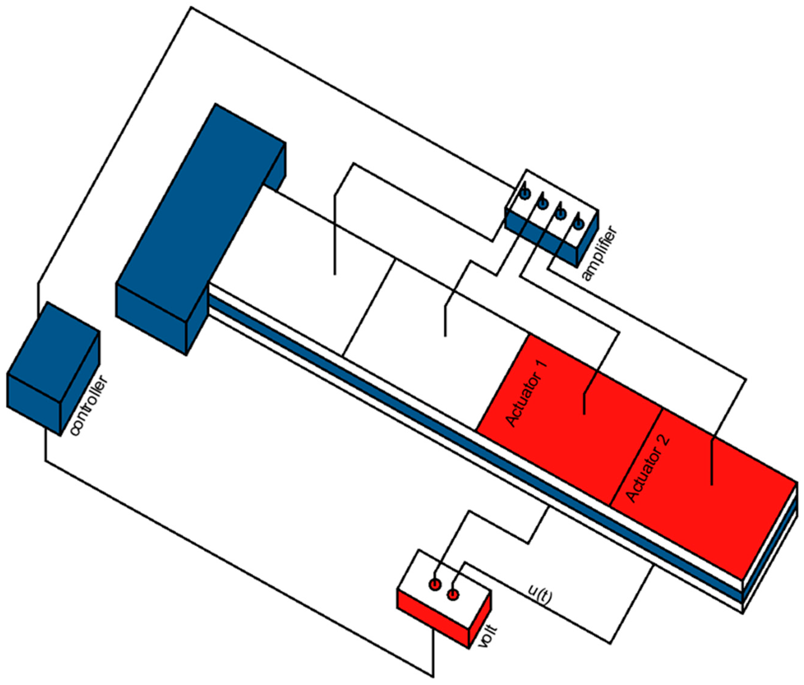
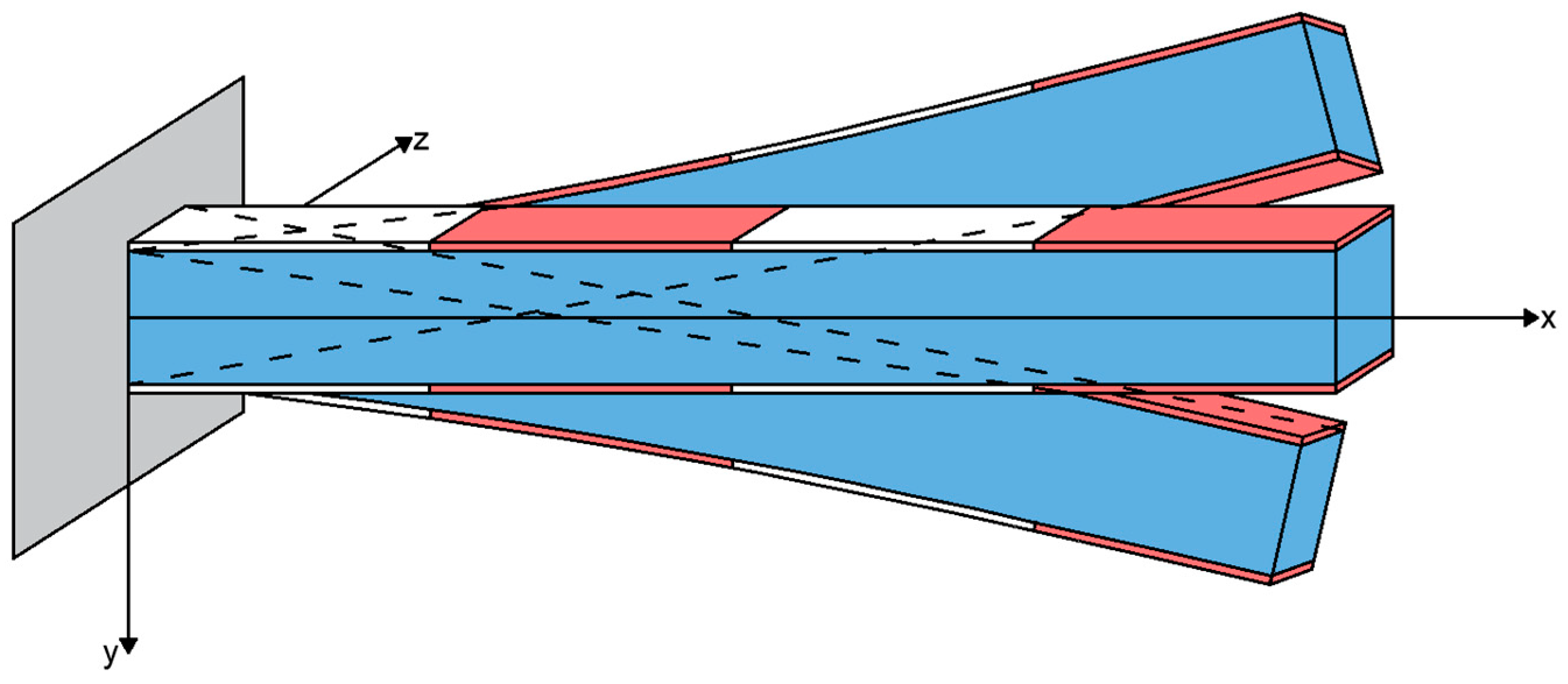
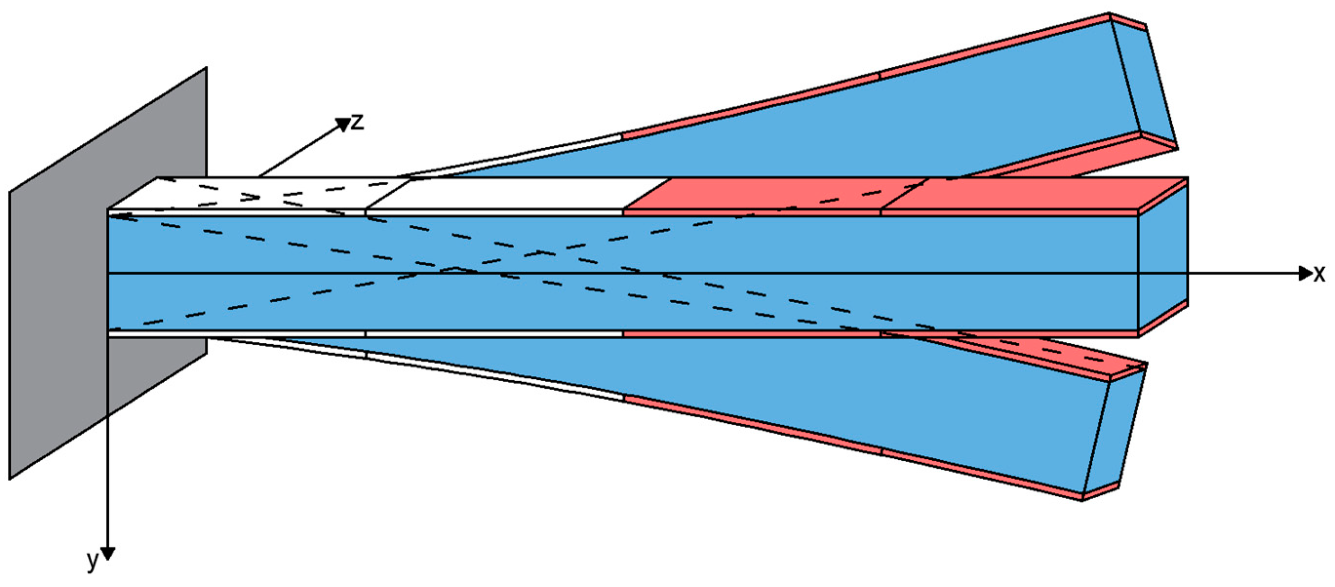
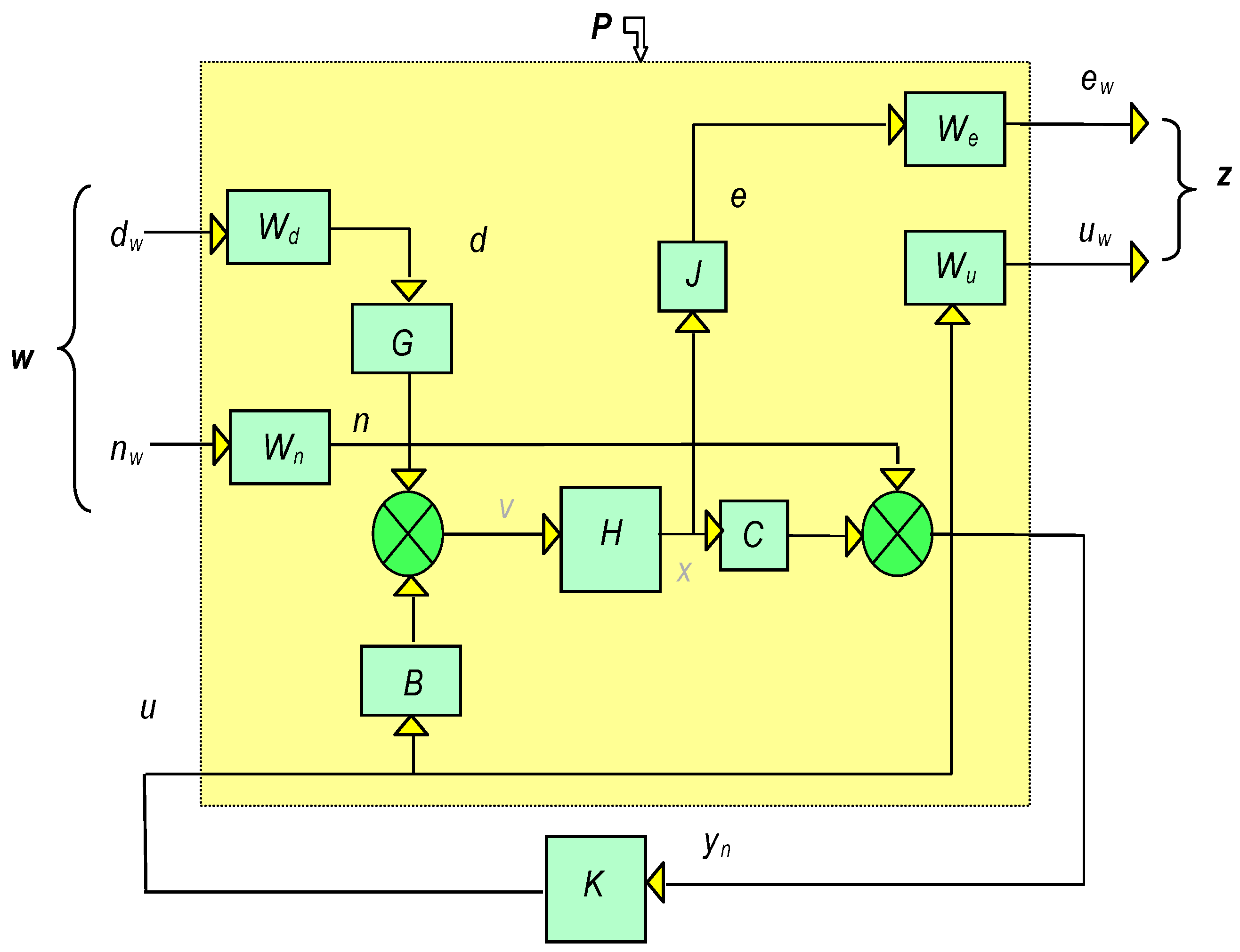
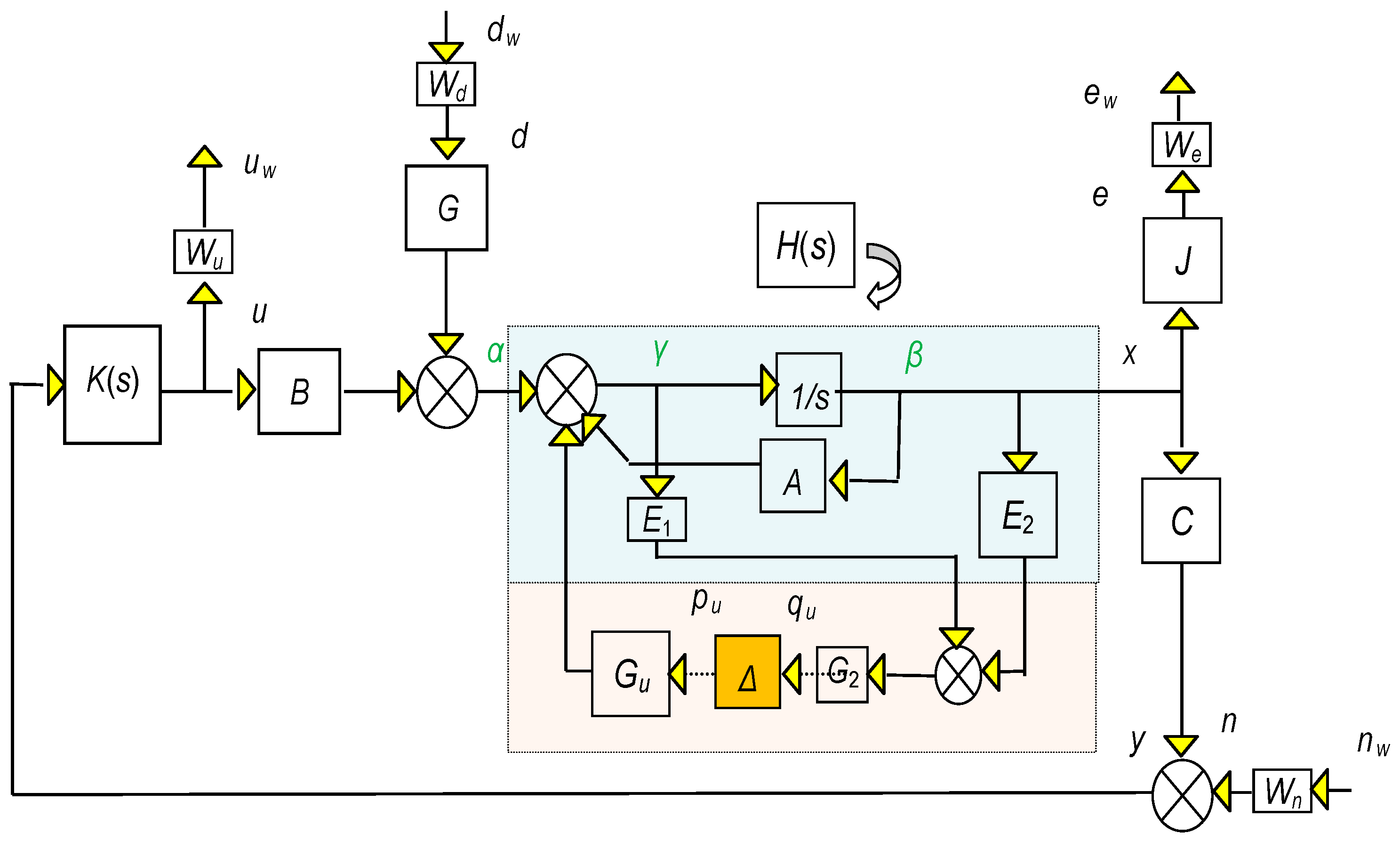
2. Modeling
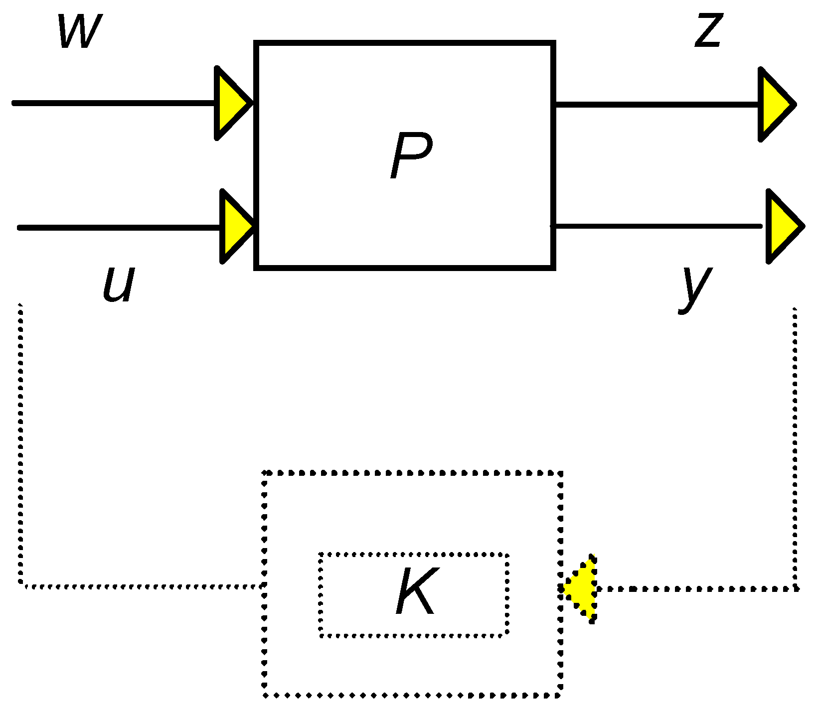
3. Controller Synthesis
- K-step. Create a controller for the scaled issue. with fixed D(s).
- D-step. Find D(jω) to minimalize at each frequency with fixed N.
- Fit the degree of each factor of D(jω) to a stable and the lowest phase transfer function D(s) and move to Step 1.
4. Results
4.1. Results in Simulation and Analysis of the Smart Structural Control
4.2. Results for the Open Loop (Initial Condition without Control)
4.3. Results with LQR Control
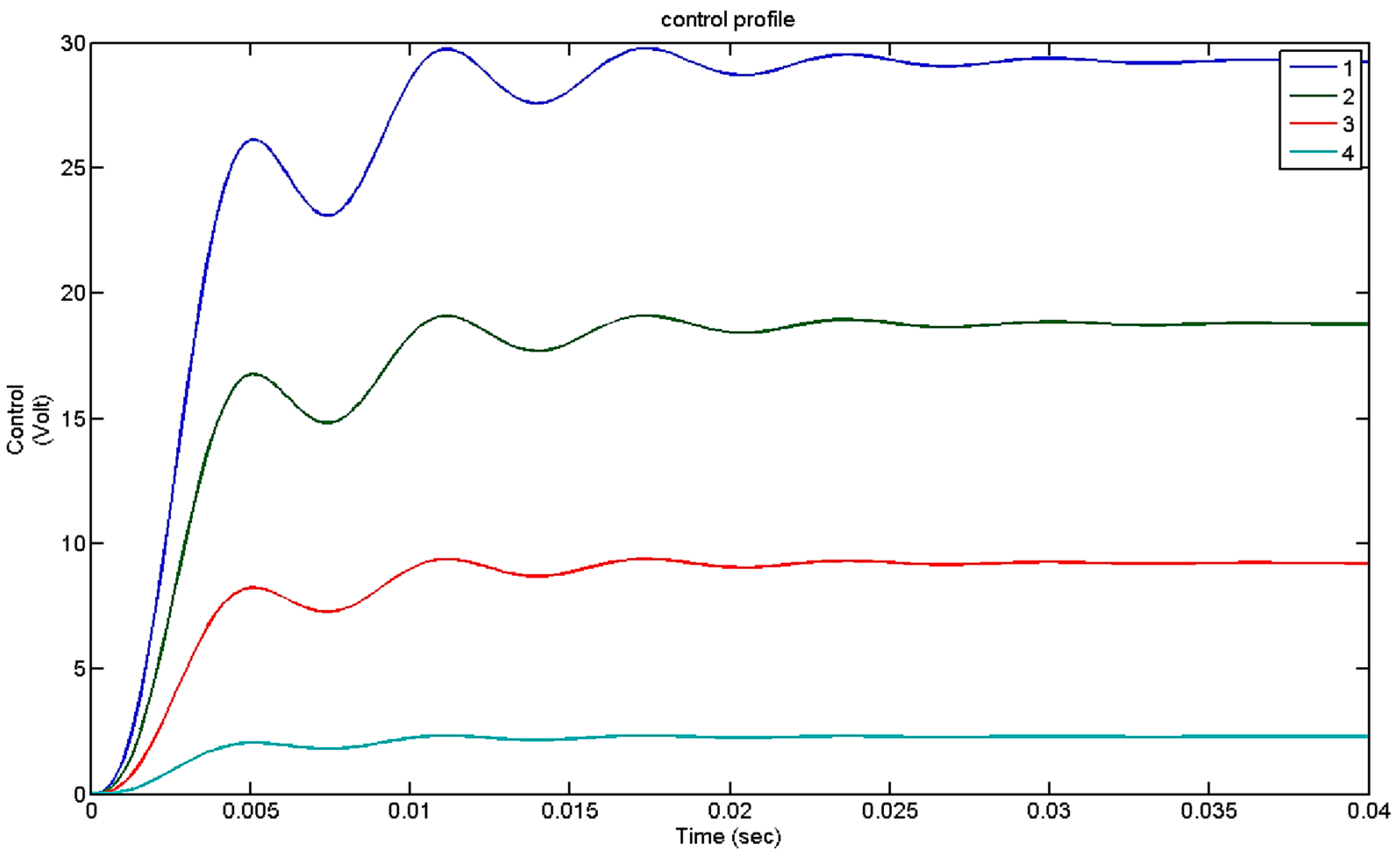
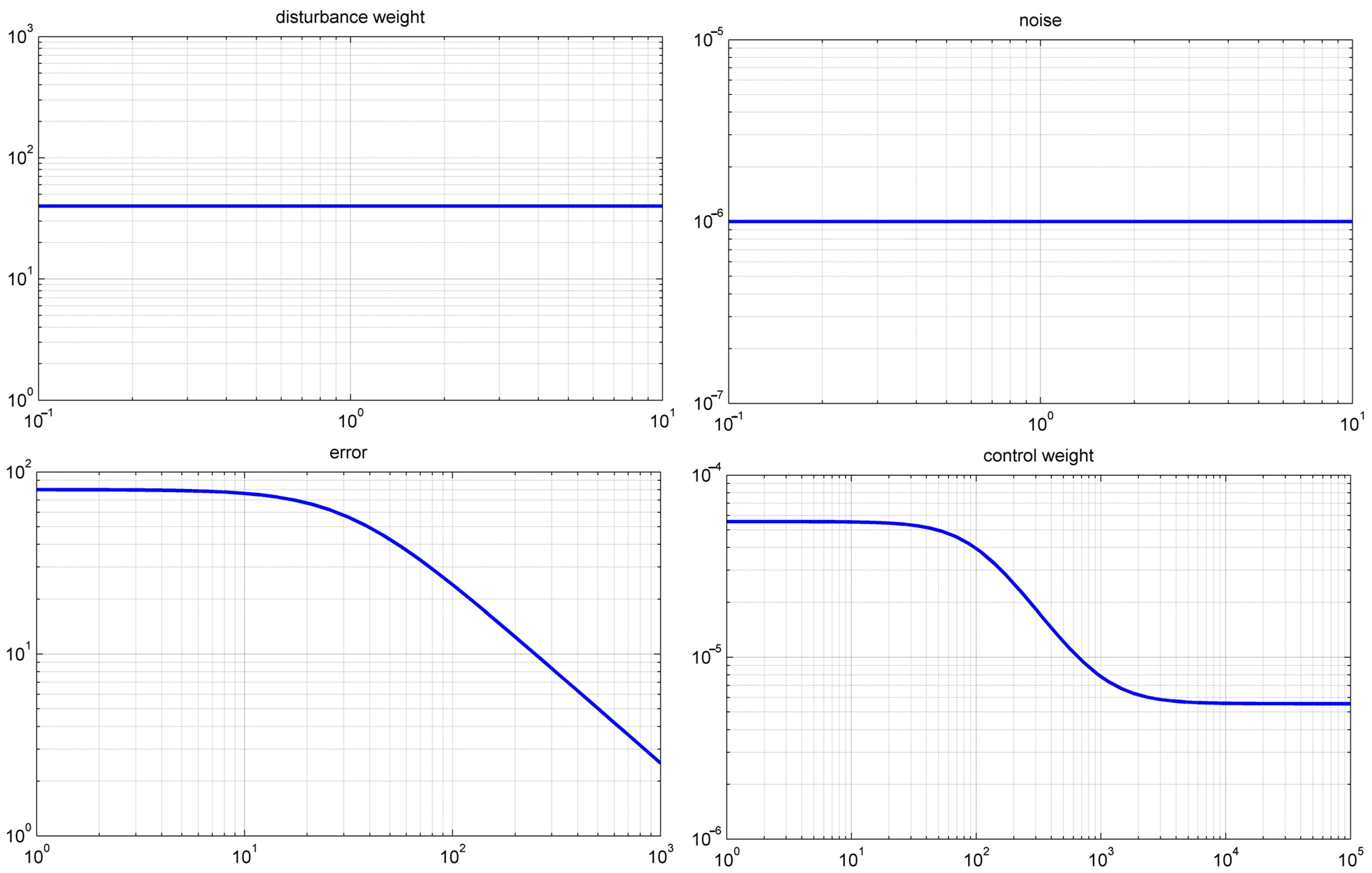
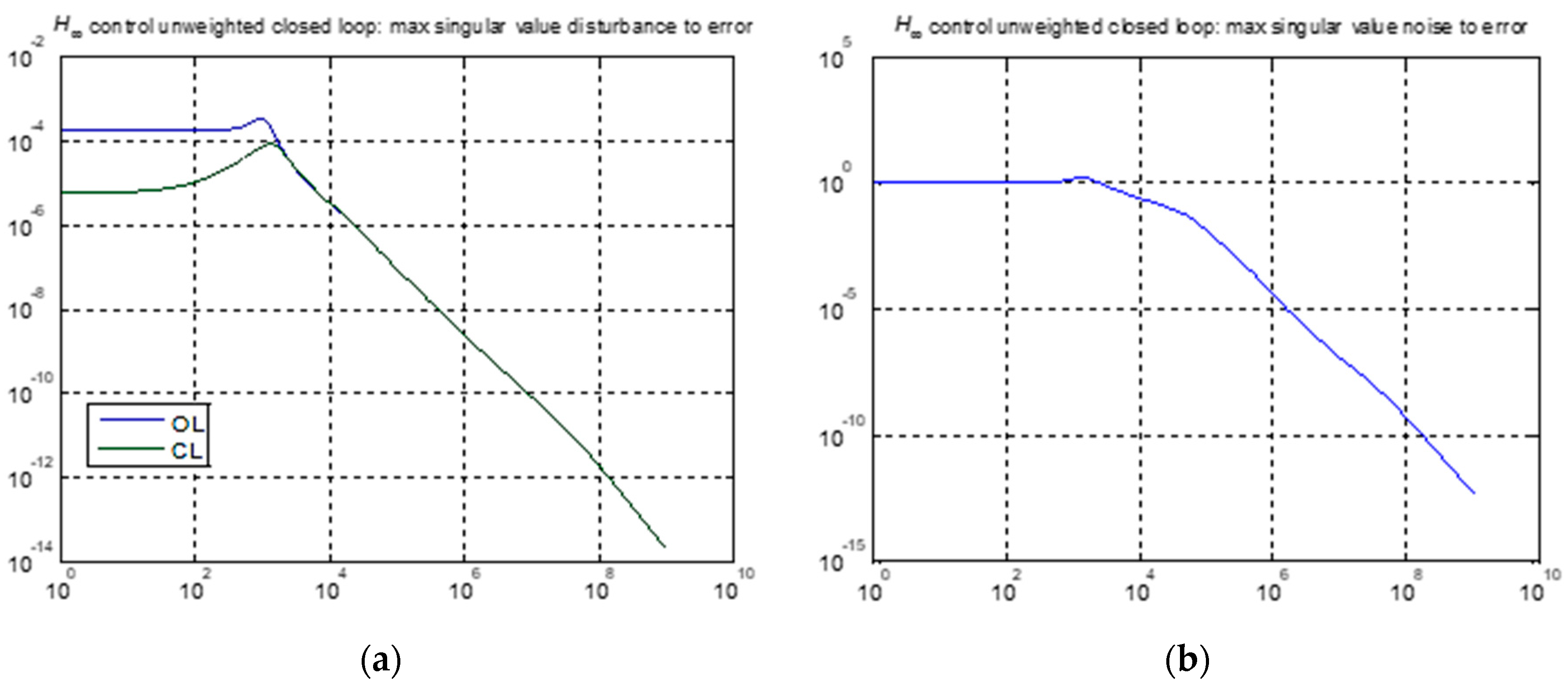
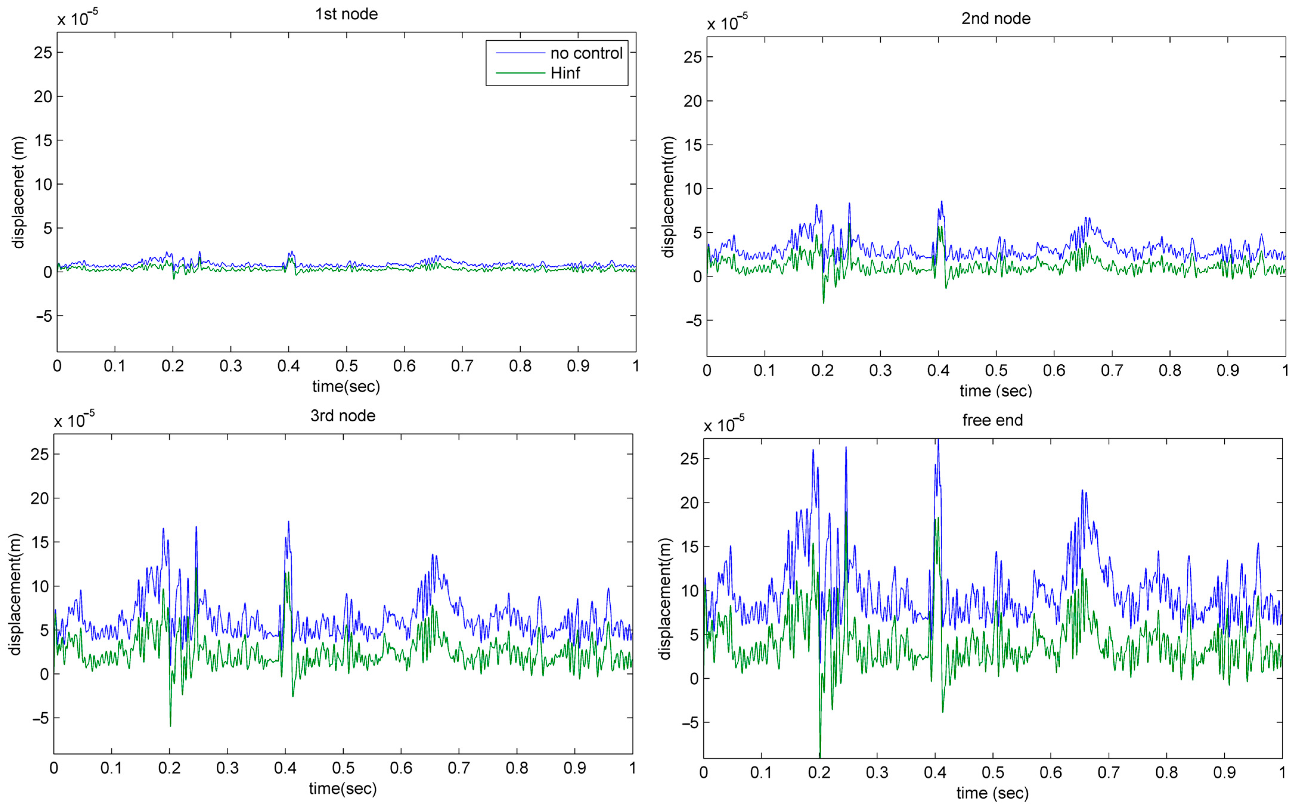
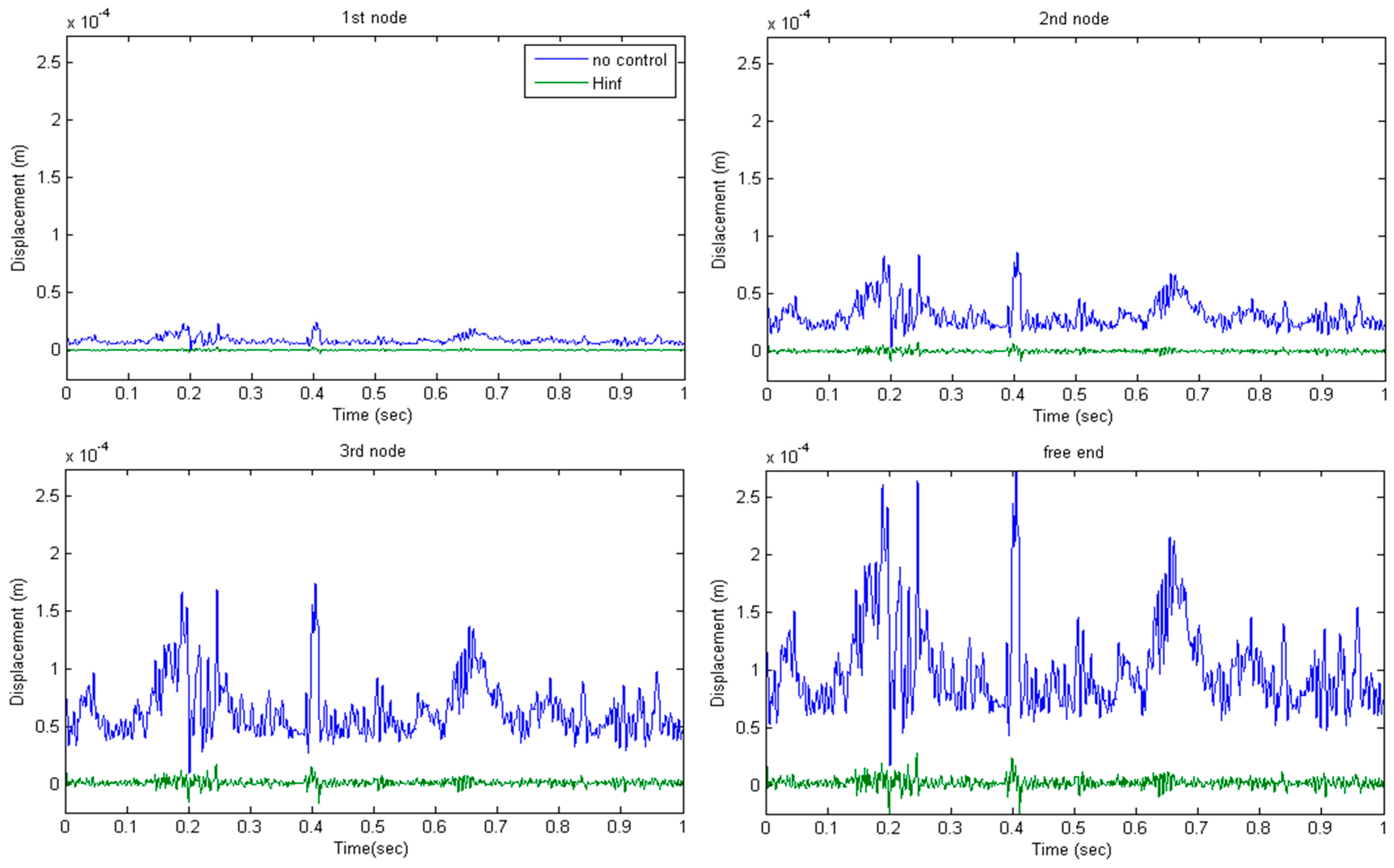
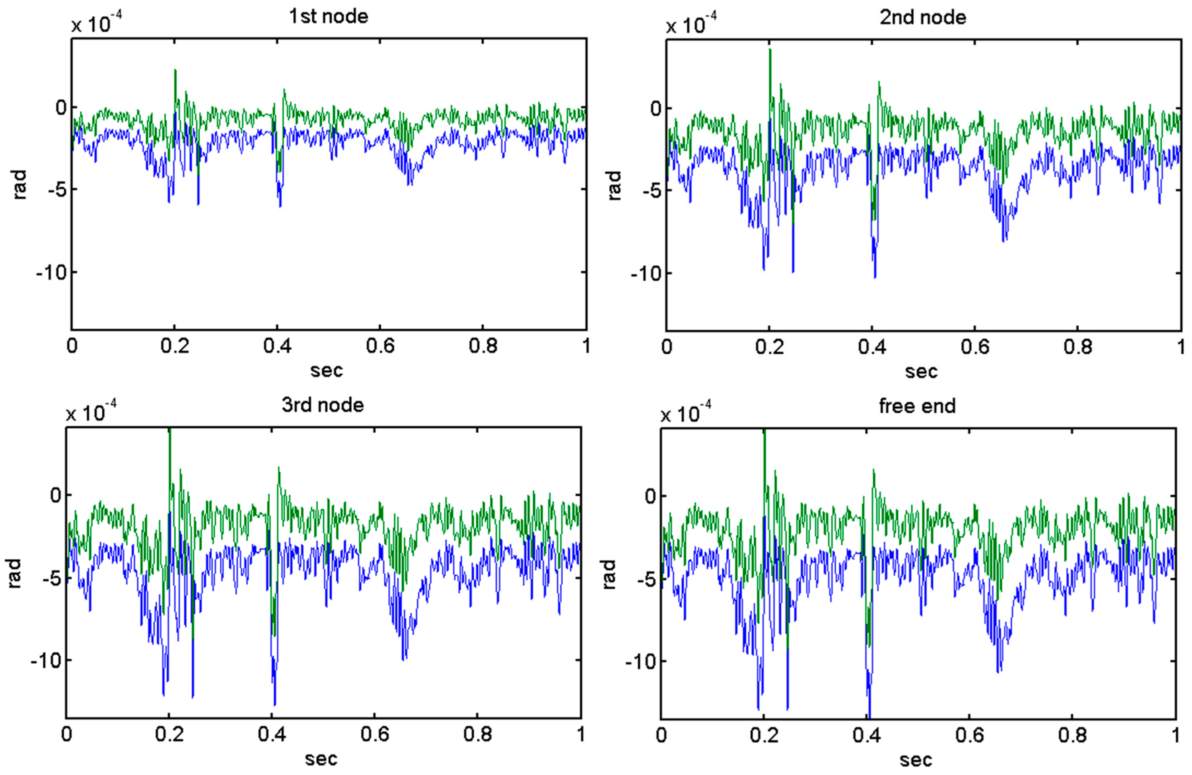
4.4. Results with Hinfinity Control
5. Discussion
- On the modeling of uncertainty in smart constructions.
- In the creation of advanced control techniques.
- In the complete suppression of vibrations under dynamic loading.
- Analytical explanation of the equations used in programming.
- Advanced programming techniques have been used to make the simulations.
- The model has been worked both in simulation and in advanced programming.
- It is not possible in one article to present both the modeling and the experimental results in such detail. For this reason, they will be presented in future research papers.
6. Conclusions
- -
- Modeling of intelligent constructs execution of control in oscillation suppression.
- -
- Using various choice places to stifle oscillations.
- -
- Results in the frequency domain as well as the time-space domain.
- -
- Introduction of the uncertainties in the construction’s mathematical model.
- -
- The integration of smart structures using methods for optimal placement and active control.
- -
- Uncertainties in dynamic loading.
- -
- Measurement noise, appropriate selection of weights for complete suppression of oscillations.
Author Contributions
Funding
Data Availability Statement
Acknowledgments
Conflicts of Interest
Nomenclature
| M | Mass Matrix | ψi(t) | Displacement deflection |
| K | Stiffness Matrix | x(t) | The state vector of our system |
| D | Viscous damping Matrix | y(t) | Output vector of our system |
| fe(t) | piezoelectric force | d31 | Piezoelectric constant |
| n | Number of nodes in finite element formulation | cp | Piezoelectric constant |
| u(t) | Control voltages of actuators | K(s) | Hinfinity Controller of the system |
| Fe | Matrix with piezoelectric constant | KlQ | LQR controller of the system |
| wi(t) | Rotation deflection | P(s) | Augment Plant of the smart system |
| μ | Singular value | e(t) | The error of the system |
| d(t) | Disturbances of the system | n(t) | Noise of the system |
| A, B, G, H | Matrices of our system | D, G-K | D-K interaction in the frequency domain |
| Tde, Tne, Tdu, Tnu | The transfer function disturbance error, noise error, disturbance control, noise control | We | The error Weight for Hinfinity control |
| Wn | The noise Weight for Hinfinity control | Wu | The control Weight for Hinfinity control |
| Wd | The disturbance Weight for Hinfinity control | N | The transfer function for the smart system |
| Δ | The Uncertainty of the system | δM t | The Uncertainty terms for the mass matrix |
| δκ | The Uncertainty terms for the stiffness matrix | kp, mp | Numerical constant from zero to one |
| J | Matrix which is utilized to select states that we are concerned with controlling | Q, R | The weight vectors for LQR control |
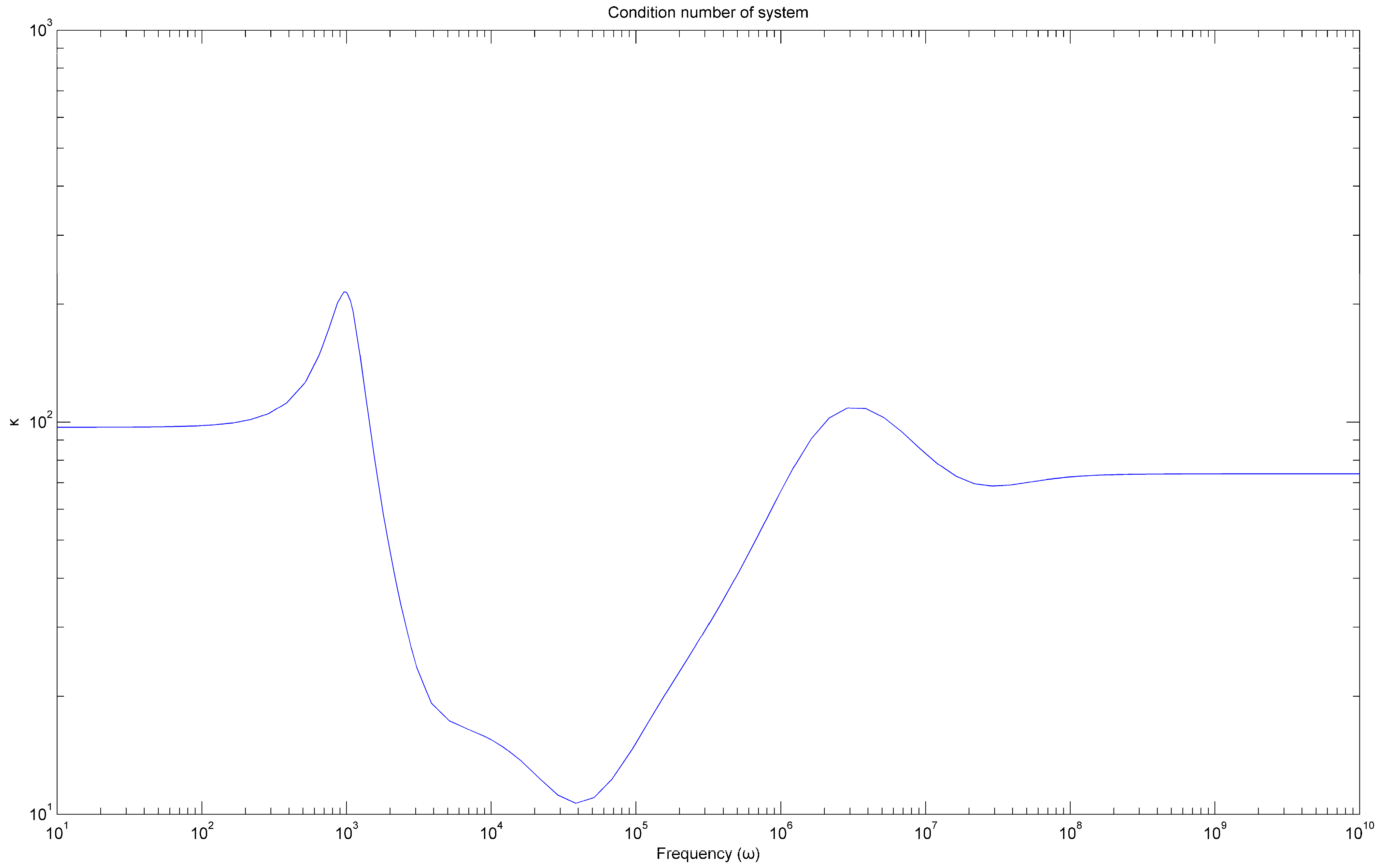
| κ(jω) | Frequency-dependent condition number | F | Fractional transformation |
References
- Tzou, H.S.; Gabbert, U. Structronics—A New Discipline and Its Challenging Issues. Fortschr.-Berichte VDI Smart Mech. Syst.—Adapt. Reihe 1997, 11, 245–250. [Google Scholar]
- Guran, A.; Tzou, H.-S.; Anderson, G.L.; Natori, M.; Gabbert, U.; Tani, J.; Breitbach, E. Structronic Systems: Smart Structures, Devices and Systems; World Scientific: Singapore, 1998; Volume 4, ISBN 978-981-02-2652-7. [Google Scholar]
- Tzou, H.S.; Anderson, G.L. Intelligent Structural Systems; Springer: London, UK, 1992; ISBN 978-94-017-1903-2. [Google Scholar]
- Gabbert, U.; Tzou, H.S. IUTAM Symposium on Smart Structures and Structronic Systems. In Proceedings of the IUTAM Symposium, Magdeburg, Germany, 26–29 September 2000; Kluwer: London, UK, 2001. [Google Scholar]
- Tzou, H.S.; Natori, M.C. Piezoelectric Materials and Continua; Elsevier: Oxford, UK, 2001; pp. 1011–1018. ISBN 978-0-12-227085-7. [Google Scholar]
- Cady, W.G. Piezoelectricity: An Introduction to the Theory and Applications of Electromechanical Phenomena in Crystals; Dover Publication: New York, NY, USA, 1964. [Google Scholar]
- Tzou, H.S.; Bao, Y. A Theory on Anisotropic Piezothermoelastic Shell Laminates with Sensor/Actuator Applications. J. Sound Vib. 1995, 184, 453–473. [Google Scholar] [CrossRef]
- Bikas, H.; Stavropoulos, P.; Chryssolouris, G. Additive Manufacturing Methods and Modelling Approaches: A Critical Review. Int. J. Adv. Manuf. Technol. 2016, 83, 389–405. [Google Scholar] [CrossRef]
- Stavropoulos, P.; Chantzis, D.; Doukas, C.; Papacharalampopoulos, A.; Chryssolouris, G. Monitoring and Control of Manufacturing Processes: A Review. Procedia CIRP 2013, 8, 421–425. [Google Scholar] [CrossRef]
- Vidakis, N.; Petousis, M.; Mountakis, N.; Papadakis, V.; Moutsopoulou, A. Mechanical Strength Predictability of Full Factorial, Taguchi, and Box Behnken Designs: Optimization of Thermal Settings and Cellulose Nanofibers Content in PA12 for MEX AM. J. Mech. Behav. Biomed. Mater. 2023, 142, 105846. [Google Scholar] [CrossRef] [PubMed]
- David, C.; Sagris, D.; Petousis, M.; Nasikas, N.K.; Moutsopoulou, A.; Sfakiotakis, E.; Mountakis, N.; Charou, C.; Vidakis, N. Operational Performance and Energy Efficiency of MEX 3D Printing with Polyamide 6 (PA6): Multi-Objective Optimization of Seven Control Settings Supported by L27 Robust Design. Appl. Sci. 2023, 13, 8819. [Google Scholar] [CrossRef]
- Moutsopoulou, A.; Stavroulakis, G.E.; Petousis, M.; Vidakis, N.; Pouliezos, A. Smart Structures Innovations Using Robust Control Methods. Appl. Mech. 2023, 4, 856–869. [Google Scholar] [CrossRef]
- Cen, S.; Soh, A.-K.; Long, Y.-Q.; Yao, Z.-H. A New 4-Node Quadrilateral FE Model with Variable Electrical Degrees of Freedom for the Analysis of Piezoelectric Laminated Composite Plates. Compos. Struct. 2002, 58, 583–599. [Google Scholar] [CrossRef]
- Yang, S.M.; Lee, Y.J. Optimization of Noncollocated Sensor/Actuator Location and Feedback Gain in Control Systems. Smart Mater. Struct. 1993, 2, 96. [Google Scholar] [CrossRef]
- Ramesh Kumar, K.; Narayanan, S. Active Vibration Control of Beams with Optimal Placement of Piezoelectric Sensor/Actuator Pairs. Smart Mater. Struct. 2008, 17, 55008. [Google Scholar] [CrossRef]
- Hanagud, S.; Obal, M.W.; Calise, A.J. Optimal Vibration Control by the Use of Piezoceramic Sensors and Actuators. J. Guid. Control Dyn. 1992, 15, 1199–1206. [Google Scholar] [CrossRef]
- Song, G.; Sethi, V.; Li, H.-N. Vibration Control of Civil Structures Using Piezoceramic Smart Materials: A Review. Eng. Struct. 2006, 28, 1513–1524. [Google Scholar] [CrossRef]
- Bandyopadhyay, B.; Manjunath, T.C.; Umapathy, M. Modeling, Control and Implementation of Smart Structures a FEM-State Space Approach; Springer: Berlin/Heidelberg, Germany, 2007; ISBN 978-3-540-48393-9. [Google Scholar]
- Miara, B.; Stavroulakis, G.E.; Valente, V. Topics on Mathematics for Smart Systems. In Proceedings of the European Conference, Rome, Italy, 26–28 October 2006. [Google Scholar]
- Moutsopoulou, A.; Stavroulakis, G.E.; Pouliezos, A.; Petousis, M.; Vidakis, N. Robust Control and Active Vibration Suppression in Dynamics of Smart Systems. Inventions 2023, 8, 47. [Google Scholar] [CrossRef]
- Zhang, N.; Kirpitchenko, I. Modelling Dynamics of a Continuous Structure with a Piezoelectric Sensoractuator for Passive Structural Control. J. Sound Vib. 2002, 249, 251–261. [Google Scholar] [CrossRef]
- Stavropoulos, P.; Manitaras, D.; Papaioannou, C.; Souflas, T.; Bikas, H. Development of a Sensor Integrated Machining Vice Towards a Non-Invasive Milling Monitoring System BT-Flexible Automation and Intelligent Manufacturing: The Human-Data-Technology Nexus; Kim, K.-Y., Monplaisir, L., Rickli, J., Eds.; Springer International Publishing: Cham, Switzerland, 2023; pp. 29–37. [Google Scholar]
- Baz, A.; Poh, S. Performance of an Active Control System with Piezoelectric Actuators. J. Sound Vib. 1988, 126, 327–343. [Google Scholar] [CrossRef]
- Moretti, M.; Silva, E.C.N.; Reddy, J.N. Topology Optimization of Flextensional Piezoelectric Actuators with Active Control Law. Smart Mater. Struct. 2019, 28, 35015. [Google Scholar] [CrossRef]
- Ma, X.; Wang, Z.; Zhou, B.; Xue, S. A Study on Performance of Distributed Piezoelectric Composite Actuators Using Galerkin Method. Smart Mater. Struct. 2019, 28, 105049. [Google Scholar] [CrossRef]
- Stavropoulos, P. Digitization of Manufacturing Processes: From Sensing to Twining. Technologies 2022, 10, 98. [Google Scholar] [CrossRef]
- Stavropoulos, P.; Souflas, T.; Papaioannou, C.; Bikas, H.; Mourtzis, D. An Adaptive, Artificial Intelligence-Based Chatter Detection Method for Milling Operations. Int. J. Adv. Manuf. Technol. 2023, 124, 2037–2058. [Google Scholar] [CrossRef]
- Ward, R.; Sun, C.; Dominguez-Caballero, J.; Ojo, S.; Ayvar-Soberanis, S.; Curtis, D.; Ozturk, E. Machining Digital Twin Using Real-Time Model-Based Simulations and Lookahead Function for Closed Loop Machining Control. Int. J. Adv. Manuf. Technol. 2021, 117, 3615–3629. [Google Scholar] [CrossRef]
- Afazov, S.; Scrimieri, D. Chatter Model for Enabling a Digital Twin in Machining. Int. J. Adv. Manuf. Technol. 2020, 110, 2439–2444. [Google Scholar] [CrossRef]
- Zhang, X.; Shao, C.; Li, S.; Xu, D.; Erdman, A.G. Robust H∞ Vibration Control for Flexible Linkage Mechanism Systems with Piezoelectric Sensors and Actuators. J. Sound Vib. 2001, 243, 145–155. [Google Scholar] [CrossRef]
- Packard, A.; Doyle, J.; Balas, G. Linear, Multivariable Robust Control with a μ Perspective. J. Dyn. Syst. Meas. Control 1993, 115, 426–438. [Google Scholar] [CrossRef]
- Stavroulakis, G.E.; Foutsitzi, G.; Hadjigeorgiou, E.; Marinova, D.; Baniotopoulos, C.C. Design and Robust Optimal Control of Smart Beams with Application on Vibrations Suppression. Adv. Eng. Softw. 2005, 36, 806–813. [Google Scholar] [CrossRef]
- Kimura, H. Robust Stabilizability for a Class of Transfer Functions. IEEE Trans. Autom. Control 1984, 29, 788–793. [Google Scholar] [CrossRef]
- Burke, J.V.; Henrion, D.; Lewis, A.S.; Overton, M.L. Stabilization via Nonsmooth, Nonconvex Optimization. IEEE Trans. Autom. Control 2006, 51, 1760–1769. [Google Scholar] [CrossRef]
- Doyle, J.; Glover, K.; Khargonekar, P.; Francis, B. State-Space Solutions to Standard H2 and H∞ Control Problems. In Proceedings of the 1988 American Control Conference, Atlanta, GA, USA, 15–17 June 1988; pp. 1691–1696. [Google Scholar]
- Francis, B.A. A Course in H∞ Control Theory; Springer: Berlin/Heidelberg, Germany, 1987; ISBN 978-3-540-17069-3. [Google Scholar]
- Friedman, Z.; Kosmatka, J.B. An Improved Two-Node Timoshenko Beam Finite Element. Comput. Struct. 1993, 47, 473–481. [Google Scholar] [CrossRef]
- Tiersten, H.F. Linear Piezoelectric Plate Vibrations: Elements of the Linear Theory of Piezoelectricity and the Vibrations Piezoelectric Plates, 1st ed.; Springer: New York, NY, USA, 1969; ISBN 978-1-4899-6221-8. [Google Scholar]
- Turchenko, V.A.; Trukhanov, S.V.; Kostishin, V.G.; Damay, F.; Porcher, F.; Klygach, D.S.; Vakhitov, M.G.; Lyakhov, D.; Michels, D.; Bozzo, B.; et al. Features of Structure, Magnetic State, and Electrodynamic Performance of SrFe12−xInxO19. Sci. Rep. 2021, 11, 18342. [Google Scholar] [CrossRef]
- Kwakernaak, H. Robust Control and H∞-Optimization—Tutorial Paper. Automatica 1993, 29, 255–273. [Google Scholar] [CrossRef]
- Chandrashekhara, K.; Varadarajan, S. Adaptive Shape Control of Composite Beams with Piezoelectric Actuators. J. Intell. Mater. Syst. Struct. 1997, 8, 112–124. [Google Scholar] [CrossRef]
- Lim, Y.-H.; Gopinathan, S.V.; Varadan, V.V.; Varadan, V.K. Finite Element Simulation of Smart Structures Using an Optimal Output Feedback Controller for Vibration and Noise Control. Smart Mater. Struct. 1999, 8, 324–337. [Google Scholar] [CrossRef]
- Zames, G.; Francis, B. Feedback, Minimax Sensitivity, and Optimal Robustness. IEEE Trans. Autom. Control 1983, 28, 585–601. [Google Scholar] [CrossRef]


| Parameters | Values |
|---|---|
| L, for Beam length | 1.00 m |
| W, for Beam width | 0.08 m |
| h, for Beam thickness | 0.02 m |
| ρ, for Beam density | 1600 kg/m3 |
| E, for Young’s modulus of the Beam | 1.5 × 10¹¹ N/m2 |
| bs, ba, for Pzt thickness | 0.002 m |
| d31 the Piezoelectric constant | 280 × 10−12 m/V |
Disclaimer/Publisher’s Note: The statements, opinions and data contained in all publications are solely those of the individual author(s) and contributor(s) and not of MDPI and/or the editor(s). MDPI and/or the editor(s) disclaim responsibility for any injury to people or property resulting from any ideas, methods, instructions or products referred to in the content. |
© 2023 by the authors. Licensee MDPI, Basel, Switzerland. This article is an open access article distributed under the terms and conditions of the Creative Commons Attribution (CC BY) license (https://creativecommons.org/licenses/by/4.0/).
Share and Cite
Moutsopoulou, A.; Stavroulakis, G.E.; Petousis, M.; Pouliezos, A.; Vidakis, N. Optimal Placement and Active Control Methods for Integrating Smart Material in Dynamic Suppression Structures. Vibration 2023, 6, 975-1003. https://doi.org/10.3390/vibration6040058
Moutsopoulou A, Stavroulakis GE, Petousis M, Pouliezos A, Vidakis N. Optimal Placement and Active Control Methods for Integrating Smart Material in Dynamic Suppression Structures. Vibration. 2023; 6(4):975-1003. https://doi.org/10.3390/vibration6040058
Chicago/Turabian StyleMoutsopoulou, Amalia, Georgios E. Stavroulakis, Markos Petousis, Anastasios Pouliezos, and Nectarios Vidakis. 2023. "Optimal Placement and Active Control Methods for Integrating Smart Material in Dynamic Suppression Structures" Vibration 6, no. 4: 975-1003. https://doi.org/10.3390/vibration6040058
APA StyleMoutsopoulou, A., Stavroulakis, G. E., Petousis, M., Pouliezos, A., & Vidakis, N. (2023). Optimal Placement and Active Control Methods for Integrating Smart Material in Dynamic Suppression Structures. Vibration, 6(4), 975-1003. https://doi.org/10.3390/vibration6040058