Deep Gaussian Process for the Approximation of a Quadratic Eigenvalue Problem: Application to Friction-Induced Vibration

Abstract

Despite numerous works over the past two decades, friction-induced vibrations, especially braking noises, are a major issue for transportation manufacturers as well as for the scientific community. To study these fugitive phenomena, the engineers need numerical methods to efficiently predict the mode coupling instabilities in a multiparametric context. The objective of this paper is to approximate the unstable frequencies and the associated damping rates extracted from a complex eigenvalue analysis under variability. To achieve this, a deep Gaussian process is considered to fit the non-linear and non-stationary evolutions of the real and imaginary parts of complex eigenvalues. The current challenge is to build an efficient surrogate modelling, considering a small training set. A discussion about the sample distribution density effect, the training set size and the kernel function choice is proposed. The results are compared to those of a Gaussian process and a deep neural network. A focus is made on several deceptive predictions of surrogate models, although the better settings were well chosen in theory. Finally, the deep Gaussian process is investigated in a multiparametric analysis to identify the best number of hidden layers and neurons, allowing a precise approximation of the behaviours of complex eigensolutions.

1. Introduction

In the last few decades, friction-induced vibration problems have been experimentally and numerically investigated and largely discussed thoroughly in the literature [1], especially for squeal problematics. This phenomenon has received the attention of both researchers and industrials in order to satisfy environmental acoustic pollution criteria and customer satisfaction. Firstly, many experimental studies at different scales were performed with experimental benchmarks to understand the squeal generation and try to reproduce it [2]. Secondly, Ouyang et al. [3] studied the impact of multiple parameters evolution in numerical simulations and concluded that the squeal phenomenon can be influenced by several parameters, such as the damping, material properties or friction coefficient. Similarly, Fritz et al. [4] highlighted that the damping can strongly affect the stability of the brake system by either modifying the friction coefficient value at which the instability appears, or by modifying the real part value, causing the instability to be modified. Similar results were obtained by Hoffman et al. [5]. Magnier et al. [6] emphasised the effects of porosity on the evolution of the friction material characteristics. By injecting these experimental results in the numerical simulations, they showed that the stability of the system is impacted as long as the contact pressure distributions. AbuBakar et al. [7] assessed the wear evolution of brake pads and highlighted that the contact interface becomes smoother and smoother as the braking duration increases. Denimal et al. [8] studied the influence of the different internal contacts of a brake system and showed that the contact formulation strongly affects the instability of the system. Graf et al. [9] emphasised that the dynamic friction formulation also modifies the stability of the system.

Nowadays, the current trend is to introduce the uncertain experimental behaviour in numerical analyses [10] and optimisation processes [11] to improve the predictivity of simulations [12]. The aim is to increase the reliability and robustness of designs by taking various kinds of uncertainty into account at the earliest stage of design. Indeed, Sarrouy et al. [13] proposed solving stochastic quadratic eigenvalue problems using intrusive polynomial chaos expansions and analysing the stability of a simplified brake squeal model as a function of variable contact stiffness and friction coefficient. Massa et al. [14] developed a numerical strategy to perform a friction-induced vibration analysis while considering model uncertainties using a fuzzy formalism. In a more targeted way, Lu et al. [15] as well as Renault et al. [16] highlighted the significant sensitivity of pad surface topographies through specific numerical simulations and experimental correlations.

To perform non-deterministic simulations previously discussed in the design step, it is important to reduce the computational time by introducing reduced-order models or surrogate models. Indeed, several authors have integrated reduction techniques to decrease the size of the studied problem, considering either homotopy developments in a projection basis [17,18], the double modal synthesis method [19,20], or a generalised modal synthesis with complex modes [21]. Other researchers focused their developments on surrogate modelling, mainly on kriging [22,23]. These works highlight the capabilities of the Gaussian process to approximate frequencies and damping rates and to perform accurate sensitivity analyses.

Machine learning methods, such as deep neural networks and deep Gaussian processes were developed and successfully used to model complex behaviours considering large training sets and to manage high dimensional problems. The interested reader can find a nice review of deep neural network in [24] and a description of the deep Gaussian process model in [25]. Recently, Stender et al. [26] proposed to use a deep neural network to detect and identify vibrations as well as to predict brake squeal. Kong et al. [27] optimised a deep neural network architecture to detect the fatigue life of automotive coil springs with high accuracy. The deep Gaussian process was used in nuclear simulations [28] to perform uncertainty propagation and parameter screening, whereas Tagade et al. [29] employed it as regression for lithium-ion battery health prognosis and degradation mode diagnosis. Next, Hebbal et al. [30] integrated a deep Gaussian process in efficient global optimization to study different mathematical problems and an aeronautic application.

The proposed study is focused on the prediction of the stability behaviour of a friction-induced vibration problem under variability. The objective is to develop and tune a surrogate model for each eigenvalue calculated with the complex eigenvalue analysis. The non-linear and non-stationary evolutions of the unstable frequencies and the associated damping rates are here approximated with a deep Gaussian process. A discussion about the sample distribution density effect, the training set size, the kernel function choice and surrogate architecture is here proposed. The obtained results are compared to those obtained by a Gaussian process and a deep neural network. Next, a focus is made on several deceptive predictions of surrogate models, although the better settings were well chosen in theory. Finally, the deep Gaussian process is investigated in a multiparametric analysis to identify the best setting allowing approximating the real and imaginary part of the complex eigenvalues efficiently.

The following sections are organised as follows. Firstly, the stability analysis of a friction-induced vibration problem and associated quadratic eigenvalue problem are discussed in Section 2. Secondly, the main concepts of each surrogate model are summarised in Section 3. Next, Section 4 highlights the performance of each surrogate model in the evaluation of a coalescence graph. Here again, the sensitivity of surrogate parameter settings and training set arrangements are studied. A focus is made on the approximation of non-linear and non-stationary functions, which gives insight into the lack of prediction. Section 5 considers a multiparametric analysis, where several parameters of the numerical model are variable. The aim is to identify the best-performing deep Gaussian process architecture, which allows characterising the behaviours of the complex eigensolutions. Finally, some conclusions about this work are drawn in the final section.

2. Resolution of a Friction-Induced Vibration Problem

2.1. Considered Model

The assessment of the capabilities and limitations of the surrogate models presented in Section 3 is done with the Double Hulten [31], shown in Figure 1.

The displacement of each mass is given along the X-axis and Y-axis. The contact between the masses and the bands is supposed to be permanent; the relation between the tangential friction force ${\mathbf{F}}_T$ and the normal friction force ${\mathbf{F}}_N$ is linear and given by the Coulomb law (Equation (1)):

$${\mathbf{F}}_T=\mu {\mathbf{F}}_N$$

(1)

Applying the classical Lagrangian formalism, the mass, damping, and stiffness matrices are determined in Equation (2).

$$\begin{array}{cccc}\hfill & \hfill \mathbf{M}=\left[\begin{array}{cccc}{m}_1& 0& 0& 0\\ 0& m_1& 0& 0\\ 0& 0& m_2& 0\\ 0& 0& 0& m_2\end{array}\right]\hfill & \hfill \mathbf{C}& \hfill =\left[\begin{array}{cccc}{c}_{12}+c_a& 0& -c_a& 0\\ 0& c_{11}& 0& 0\\ -c_a& 0& c_{22}+c_a& 0\\ 0& 0& 0& c_{21}\end{array}\right]\hfill \\ \\ \hfill {\mathbf{K}}_{\Sigma }& \hfill =\left[\begin{array}{cccc}{k}_{12}+k_a& 0& -k_a& 0\\ 0& k_{11}& 0& 0\\ -k_a& 0& k_{22}+k_a& 0\\ 0& 0& 0& k_{21}\end{array}\right]\hfill & \hfill {\mathbf{K}}_{NL}& \hfill =\left[\begin{array}{cccc}0& \mu k_{11}& 0& 0\\ -\mu k_{12}& 0& 0& 0\\ 0& 0& 0& \mu k_{21}\\ 0& 0& -\mu k_{22}& 0\end{array}\right]\hfill \end{array}$$

(2)

The parameters of the Double Hulten are split into two categories: the system and the contact parameters. Their reference values are recalled in

Table 1. Nominal value of the system parameters of the Double Hulten.

m${}_1$	m${}_2$	k${}_{11}$	k${}_{12}$	k${}_{21}$	k${}_{22}$	k${}_{\mathit{a}}$	c${}_{11}$	c${}_{12}$	c${}_{21}$	c${}_{22}$	c${}_{\mathit{a}}$
(kg)	(kg)	(N/m)	(N/m)	(N/m)	(N/m)	(N/m)	(Ns/m)	(Ns/m)	(Ns/m)	(Ns/m)	(Ns/m)
1	1	3000	6000	1000	3000	1000	1	1	1	1	1

.

To determine the eigensolutions (${\lambda }_i$,${\mathit{\psi }}_i$) of the system, the QEP (Equation (3)) is solved with the well-known QZ algorithm, where the mass $\mathbf{M}$, damping $\mathbf{C}$ and stiffness $\mathbf{K}$ matrices are given in Equation (2).

$$\left({\lambda }_i^2\mathbf{M}+{\lambda }_i\mathbf{C}+\mathbf{K}\right){\mathit{\psi }}_i=\mathbf{0}$$

(3)

where $\mathbf{K}={\mathbf{K}}_{\Sigma }+{\mathbf{K}}_{NL}$.

The coalescence graph of this model when considering the nominal parameters presented in Table 1 is given in Figure 2. Three mode couplings are respectively detected for friction coefficients of 0.2, 0.57 and 0.84.

The imaginary part evolutions of the model eigenvalues are relatively smooth and present small nonlinearities. Conversely, the real part evolutions of the model eigenvalues are more complex and exhibit non-stationary behaviour. Indeed, for instance, the first real part eigenvalue is constant on the majority of the design space, except when the friction coefficient $\mu$ is greater than 0.8.

From all eight functions (real and imaginary parts), the second and the third eigenvalues represent the highest level of complexity. Nonetheless, to efficiently compare the capabilities and limitations of the considered surrogate model techniques, all of these functions are considered in this sequel.

2.2. Mode Pairing Strategy

Traditionally, the mode pairing strategy hinges on the MAC, given by Equation (4).

$${\mathrm{MAC}}_{ik}=\frac{{∥{\psi }_i^{*(n+1)H}{\psi }_k^{*\left(n\right)}∥}^2}{∥{\psi }_i^{*(n+1)H}{\psi }_i^{*(n+1)}∥∥{\psi }_k^{*\left(n\right)H}{\psi }_k^{*\left(n\right)}∥}$$

(4)

where ${\psi }_i$ is the ith eigenvector of the considered system.

When considering a multiparametric analysis, the strategy is to compare all eigenvectors ${\mathit{\psi }}_j$ with a reference set of eigenvectors (for instance, the nominal values of the parameters of the multiparametric analysis, ${\widehat{P}}_0$) and construct a family ${\mathcal{F}}_i$ for each mode of the system.

The first limitation comes from the reference set of parameter values ${\widehat{P}}_0$. To be fully efficient, ${\widehat{P}}_0$ must be quite close, in the MAC sense, to any set of parameter values $\widehat{P}$ of the design space $\mathcal{D}$.

Figure 3 shows a comparison between two families (circled in gray), generated with two different reference sets of parameter values ${\widehat{P}}_0$, depicted by a red star. The blue dots represent the evaluated configurations ${\psi }_k$, and the black arrows represent a pairing with MAC values greater than the threshold. Figure 3a shows a good choice for the reference set ${\widehat{P}}_0$ since the given set is close to any member of the eigenforms ${\psi }_k$. Conversely, Figure 3b exhibits a poor choice since four configurations are not included into the family $\mathcal{F}$.

The FIV problems are highly subjected to mode veering [32], which appears when modes are coupled with each other. The veering is characterised by modes which approach each other and suddenly veer away. Before the veering, the shape of mode 1 and mode 2 are respectively given by ${\varphi }_1$ and ${\varphi }_2$. The modal form at the loci is a linear combination of ${\varphi }_1$ and ${\varphi }_2$. After the veering, mode 1 is characterised by shape ${\varphi }_2$, and mode 2 by ${\varphi }_1$.

In practice, choosing a veering shape to initialise the pairing strategy creates only one family. To prevent this issue, the reference has to be a modal form, which is not in a superposed state (either before or after the veering). For squeal problems, only the normal contact state ($\mu$ = 0) has the highest probability to be veering free. Finally, the other parameters are set to the nominal values since the uncertainties are always defined around these values.

However, these conditions place the strategy in the state of Figure 3b, where some configurations are not paired. To counterbalance this issue, the pairing process is executed iteratively: first, the process is computed with the red star reference set ${\widehat{P}}_0$. Then, the configurations ${\psi }_k$, which have just been paired, are added to the reference set ${\widehat{P}}_0$. This set is thus composed of four reference configurations for the given example of Figure 3b. The pairing process is started again until all configurations are successfully added to the reference set ${\widehat{P}}_0$ to create the family $\mathcal{F}$.

3. Surrogate Modelling Theory

3.1. Surrogate Principle

The main idea behind surrogate modelling is to approximate an expensive function $f:\mathcal{D}\to \mathcal{E}$, where $\mathcal{D}={\prod }_{i=1}^D\left[L_i;U_i\right]$, and $\mathcal{E}$ is the image of $\mathcal{D}$ through the mapping function f with a cheaper model. The variable D represents the number of input parameters, whereas $L_i$ and $U_i$ are respectively the lower and upper bounds of the ith dimension. $\mathcal{D}$ and $\mathcal{E}$ are respectively subsets of ${\mathbb{R}}^D$ and $\mathbb{R}$. To construct an approximation of the considered function, the surrogate model hinges on the acquisition of a priori knowledge. This a priori knowledge is given by a training set, from which the statistical relationship between the inputs and the outputs is deduced.

Let $\mathcal{T}$ be a training set such as $\mathcal{T}=\left\{(x_i,y_i)\right|i\in [1,n]$}, where ${\mathbf{x}}_i$ denotes an input vector of ($1\times D$) dimension, and $y_i$ is a scalar corresponding to the image of ${\mathbf{x}}_i$ through f. In addition, the matrix $\mathbf{X}\in {\mathcal{M}}_{n,D}$ and the vector $\mathcal{Y}\in {\mathbb{R}}^n$ contain all the inputs and outputs of the training set $\mathcal{T}$.

First, the training set is defined using a space filling strategy, such as the LHS [33], and the evaluation of this training set through a simulator. Then, the surrogate model is chosen, and its parameters are defined. They are commonly divided into two categories: the fixed ones and the optimised ones. The distinction is done through the consideration of several hypotheses about the training set and the given simulator. Finally, the surrogate model is fed with the information from the training set to carry out the predictions.

For a fixed training set, the prediction efficiency and time computation of a surrogate model is clearly dependent on the setting of its parameters. Consequently, the techniques used to tune these data are presented in the following subsections for both surrogate models. Throughout this sequel, the fixed parameters are denoted as hyperparameters, as they can be denoted in the literature, and the optimised parameters are simply denoted as parameters.

3.2. Gaussian Process

A GP [34] is a stochastic process G, indexed by a set $\mathbb{X}\subset {\mathbb{R}}^D$, such that any finite number of random variables is jointly Gaussian: $\forall p\in {\mathbb{N}}^{*},\forall \mathbf{X}={[{\mathbf{X}}_1,\cdots ,{\mathbf{X}}_p]}^T,\mathbf{G}\left(\mathbf{X}\right)\sim \mathcal{N}(\mu \left(\mathbf{X}\right),\mathbf{C}(\mathbf{X},\mathbf{X}))$ with $\mathbf{G}\left(\mathbf{X}\right)={[\mathbf{G}\left({\mathbf{X}}_1\right),\cdots \mathbf{G}\left({\mathbf{X}}_p\right)]}^T$, where $\mu (·)$ and $\mathbf{C}(·,·)$ respectively stand for the mean and covariance function of the GP. Using a GP as a surrogate model consists in considering the output prediction, denoted by the random variable $\widehat{\mathbf{Y}}$ as a realisation of this stochastic process.

Since $\widehat{\mathbf{Y}}$ is also Gaussian, its density function is described by its first two momenta $\widehat{\mu }$ and $\widehat{s}$, given respectively by Equations (5) and (6).

$$\begin{array}{c}\hfill \widehat{\mu }\left({\mathbf{x}}_{*}\right)=\mu \left({\mathbf{x}}_{*}\right)+\mathbf{C}({\mathbf{x}}_{*},\mathbf{X}){\left[\mathbf{C}(\mathbf{X},\mathbf{X})+{\sigma }_n^2\mathbf{I}\right]}^{-1}(\mathbf{y}\left(\mathbf{X}\right)-\mu \left(\mathbf{X}\right))\end{array}$$

(5)

$$\begin{array}{c}\hfill \widehat{s}\left({\mathbf{x}}_{*}\right)=\mathbf{C}({\mathbf{x}}_{*},{\mathbf{x}}_{*})-\mathbf{C}({\mathbf{x}}_{*},\mathbf{X}){\left[\mathbf{C}(\mathbf{X},\mathbf{X})+{\sigma }_n^2\mathbf{I}\right]}^{-1}\mathbf{C}(\mathbf{X},{\mathbf{x}}_{*})\end{array}$$

(6)

where ${\mathbf{x}}_{*}$ is any vector defined in $\mathcal{D}$, $\mu$ is the mean of the GP, $\mathbf{C}$ is its covariance function, ${\sigma }_n^2$ is the noise of the data, and I is the identity matrix.

Next, considering the covariance function defined by Equation (7).

$$\mathbf{C}({\mathbf{x}}_r,{\mathbf{x}}_s)={\sigma }_k^2\mathbf{K}({\mathbf{x}}_r,{\mathbf{x}}_s)$$

(7)

where $(r,s)\in {[1;n]}^2$, ${\sigma }_k^2$ is the signal variance (also called the noise of the kernel) and $\mathbf{K}$ is the correlation matrix (also called the kernel function or kernel matrix).

Table 2. Kernel functions.

Type of Kernel Functions	$\mathbf{K}({\mathbf{x}}_{\mathit{r}},{\mathbf{x}}_{\mathit{s}})$
Matern 3/2	$\left(1+\sqrt{3}|{\mathbf{x}}_r,{\mathbf{x}}_s|\right)exp\left(-\sqrt{3}|{\mathbf{x}}_r,{\mathbf{x}}_s|\right)$
Matern 5/2	${\left(1+\sqrt{5}|{\mathbf{x}}_r,{\mathbf{x}}_s|+\frac{5}{3}|{\mathbf{x}}_r,{\mathbf{x}}_s|\right)}^{2}exp\left(-\sqrt{5}|{\mathbf{x}}_r,{\mathbf{x}}_s|\right)$
Exponential quadratic	$exp\left(-|{\mathbf{x}}_r,{\mathbf{x}}_s{|}^2\right)$

presents the most common choice for the kernel function. They are presented from the least smooth to the smoothest. This property has a direct impact on the approximation of functions. Indeed, the smoothness drives the GP prediction: the more the kernel is non-smooth, the greater the non-linearity of the prediction will be.

$|{\mathbf{x}}_r,{\mathbf{x}}_s|:=\sqrt{\left({\displaystyle \sum _{i=1}^D\frac{{(x_{(r,i)}-x_{(s,i)})}^2}{{\theta }_i^2}}\right)}$ represents the weighted Euclidean distance with ${\theta }_i$ being a weight coefficient, called the lengthscale, allowing increasing or reducing the importance of a dimension.

For the estimation of the parameters of a linear model, the best linear unbiased estimator equals the minimum variance unbiased (or MVU) if the noise is Gaussian. For the linear Gaussian model, the maximum likelihood estimator (hereby denoted MLE) is equivalent to the MVU estimator. Here, we follow the common way to optimise the GP parameters through the model evidence $f_{\left(Y\right|X)}$, which is the multivariate probability density function of the random variable Y, given the random variable X. This function is supposed to be the Gaussian of mean $\mu \left(X\right)$ and of variance $\mathbf{C}(\mathbf{X},\mathbf{X})+{\sigma }_n^2\mathbf{I}$, and it is traditionally optimised to obtain the MLE by updating the value components of the lengthscale vector. To ease the optimisation process, the log form of the probability density function is considered and gives the Equation (8). At last, non-Gaussian behaviours (e.g., positivity, heterogeneity, and discontinuities) could be captured by the physically informed kernels, and this approach could be the subject of future work.

$$Loss\left(\mathsf{\Theta }\right)=-\frac{n}{2}log\left(2\pi \right)-\frac{1}{2}log(det(\mathbf{C}+{\sigma }_n^2\mathbf{I}))-\frac{1}{2}\left(({\mathbf{y}}^T-\mu \left(\mathbf{X}\right)){\left(\mathbf{C}+{\sigma }_n^2\mathbf{I}\right)}^{-1}(\mathbf{y}-\mu \left(\mathbf{X}\right))\right)$$

(8)

where $\mathsf{\Theta }$ is the vector of lengthscale.

The second term of the sum is the regularisation coefficient that prevents the GP from overfitting. The third term of the sum corresponds to the terms that try to fit the data.

The different surrogate parameters (hyperparameters and parameters) considered for the GP are summarised in

Table 3. GP parameter and hyperparameters.

Name of the Quantity	Nature of the Quantity	Associated Variable	Equation
Data noise	Hyperparameter	${\sigma }_n^2$	Equation (5)
Mean function	Hyperparameter	$\mu$	Equation (5)
Signal variance	Hyperparameter	${\sigma }_k^2$	Equation (7)
Kernel function	Hyperparameter	$\mathbf{K}$	Table 2
Lengthscale	Parameter	$\mathsf{\Theta }$	Equation (8)

.

3.3. Deep Neural Network

A DNN [35] is a deterministic surrogate model composed of artificial neurons. An artificial neuron corresponds to a coarse and over-simplified version of a brain neuron, called a perceptron, and aims at mimicking the biological phenomenon that generates a signal between two neurons. A DNN is then obtained by connecting perceptrons with each other and organising them in layers.

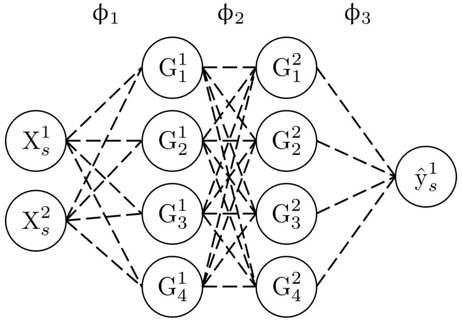
Figure 4 shows an example of a neural network architecture. In this case, the input dimension d is 2, and the output dimension is 1. There are two intermediate layers, each composed of four neurons. The input neurons on the left are associated with the input data (labelled $X_s^d$), whereas the output neuron on the right is associated with the output data (labelled ${\widehat{y}}_s^1$). The value of a neuron on the intermediate layers is determined by carrying the linear combinations of the connected neurons from the previous layer and then applying an activation function (Equation (9)).

$$G_i^{D^{\left(i\right)}}={\mathsf{\varphi }}_i\left({\mathbf{w}}_{i-1}^T{\mathbf{G}}^{i-1}\right)$$

(9)

where $i\in [1;p]$, p is the number of hidden layers, $D^{\left(i\right)}$, the number of neurons per hidden layer, ${\mathsf{\varphi }}_i$ is the activation function of the ith hidden layer, ${\mathbf{w}}_i={[w_i^1\cdots w_i^j\cdots w_i^{D^{\left(i\right)}}]}^T$ is the weight vector associated with the ith hidden layer, and $\mathbf{G}=[G_{inonlinear1}^1\cdots G_{i-1}^j\cdots$$G_{i-1}^{D^{(i-1)}}{]}^T$ is the neuron vector associated with the previous hidden layer.

The most common activation functions used in DNN are summarised in

Table 4. Common activation functions.

Type of Activation Function	$\mathsf{\varphi }\left(\mathit{x}\right)$
ReLU	$max(0,x)$
Hyperbolic tangent	$tanh\left(x\right)$
Logistic	$\frac{1}{1+exp(-x)}$

. These functions, coupled with the architecture of the neural network, allow capturing the full complexity of the considered functions. Nielsen [36] proved that one characteristic of this surrogate model is that it is a universal approximator. Nevertheless, this strength is also one of its biggest weaknesses. Indeed, this capacity to increase the complexity of the learning via the increase in neurons in hidden layers can lead to overfitting [37]. Typically, this overfitting phenomenon is associated with weight values, which are too high. One way to try to remove this flaw is penalising the weight values with a regularisation coefficient, such as in Equation (10).

$${\displaystyle Loss\left(\mathbf{W}\right)=\frac{1}{2n}\sum _{i=1}^n{(y_i-{\widehat{y}}_i)}^2+\frac{\alpha }{2}\sqrt{\left({\displaystyle \sum _{k=1}^p\sum _{j=1}^{D^{\left(k\right)}}{W}_{j,k}^2}\right)}}$$

(10)

where $\mathbf{W}=[{\mathbf{w}}_1\cdots {\mathbf{w}}_k\cdots {\mathbf{w}}_p]$ is the coefficient matrix for which each column corresponds to the coefficient vector from the ith hidden layer and $\alpha$ the regularisation coefficient.

The Equation (10) gives the loss function used for the neural network. This equation is equivalent to the least squares method with an additional contribution, which allows controlling overfitting. This control is done by adding all the weight values together and multiplying them with a coefficient, which modifies the impact of the sum on the loss function. Typically, from the observations made on these considered functions, a value of $\alpha$ lower than 0.005 corresponds to a small regularisation, between 0.005 and 0.05 corresponds to a medium regularisation, and a value above 0.05 corresponds to a strong regularisation. This hyperparameter has to be tuned cautiously since a high value prevents the surrogate model from going through the training set points, inducing important error values, and a small value increases the chance of overfitting.

The optimisation of the weight values linking the different neurons is done via the backpropagation procedure. First, the weight values are initialised randomly. Then, the loss function is computed and minimised using a classical gradient descent algorithm. In this research, since the data are scarce, the optimisation is ensured by an L-BFGS (limited-memory Broyden–Fletcher–Goldfard–Shanno) algorithm [38].

Once the weight matrix is optimised, the prediction is carried with the Equation (11).

$$\widehat{y}\left({\mathbf{x}}_{*}\right)={\mathsf{\varphi }}_p\left({\mathsf{\varphi }}_{p-1}(\cdots \left({\mathsf{\varphi }}_1\left({\mathbf{w}}_1{\mathbf{x}}_{*}\right)\right)\cdots )\right)$$

(11)

Table 5. DNN parameters and hyperparameters.

Name of the Quantity	Nature of the Quantity	Associated Variable	Equation
Activation function	Hyperparameter	$\mathsf{\varphi }$	Table 4
Weight matrix	Parameter	$\mathbf{W}$	Equation (9)
Number of hidden layers	Hyperparameter	p	Equation (11)
Number of neurons per hidden layer	Hyperparameter	$D^{\left(i\right)}$	Equation (9)
Regularisation coefficient	Hyperparameter	$\alpha$	Equation (10)

summarises the different quantities considered in the DNN surrogate model.

3.4. Deep Gaussian Process

The DGP is a recent class of surrogate models [25] and is inspired by the deep learning theory. The main idea is to capture complex variations of the underlying function by decomposing the information embedded in the training set, i.e., through nested structures. Thus, the DGP hinges on neurons and layers, being a stack of GPs.

Hence, a random vector ${\mathbf{H}}^{\ell }$ (Equation (13)) is introduced for each layer of the DGP. This random vector is defined by a GP ${\mathbf{G}}^{\ell }$ given by Equation (12). This prior hinges on the fundamental assumption that the current layer is only conditionally dependent on the previous layer random vector ${\mathbf{H}}^{\ell -1}$.

$${\mathbf{G}}^{\ell }\left({\mathbf{H}}^{\ell -1}\right)\sim \mathcal{N}(\mu \left({\mathbf{H}}^{\ell -1}\right),C({\mathbf{H}}^{\ell -1},{\mathbf{H}}^{\ell -1}))$$

(12)

for $\ell \in [1,L]$, ${\mathbf{H}}^0=\mathbf{X}$ and L is the number of hidden layers. $\mu$ and C are respectively the mean and the covariance function of the ℓth layer.

$${\mathbf{H}}^{\ell }=\left[\begin{array}{ccccc}{H}_{1,1}^{\ell }& \cdots & H_{1,j}^{\ell }& \cdots & H_{1,D^{(\ell )}}^{\ell }\\ ⋮& \ddots & ⋮& \ddots & ⋮\\ H_{i,1}^{\ell }& \cdots & H_{i,j}^{\ell }& \cdots & H_{i,D^{(\ell )}}^{\ell }\\ ⋮& \ddots & ⋮& \ddots & ⋮\\ H_{n,1}^{\ell }& \cdots & H_{n,j}^{\ell }& \cdots & H_{n,D^{(\ell )}}^{\ell }\end{array}\right]$$

(13)

where $D^{(\ell )}$ is the number of neurons per hidden layer.

These priors are quite expensive to compute since they involve an inversion of the covariance matrix $\mathbf{C}({\mathbf{H}}^{\ell -1},{\mathbf{H}}^{\ell -1}))$, which is $\mathcal{O}\left(n^3\right)$ for each layer of the surrogate model. To reduce the computational cost of the matrix inversion, the pseudo-inputs [39] (also called inducing points in the literature) are introduced. The main idea behind this trick is to increase the probability space with non-observed points which will, to a certain extent, summarise the data and reduce the cost of the inversion to $\mathcal{O}\left(m^3\right)$, where m is the number of pseudo-inputs. For significant effects, m has to be a lot smaller than n when considering large training sets. If the number of samples is small, this number can be chosen with more flexibility.

For each layer, a random vector ${\mathbf{U}}^{\ell }$ and a set of pseudo-inputs, denoted as ${\mathbf{Z}}^{\ell }$, are introduced. The random vector ${\mathbf{U}}^{\ell }$ is defined using the aforementioned GP (Equation (14)).

$${\mathbf{G}}^{\ell }\left({\mathbf{Z}}^{\ell -1}\right)\sim \mathcal{N}(\mu \left({\mathbf{Z}}^{\ell -1}\right),C({\mathbf{Z}}^{\ell -1},{\mathbf{Z}}^{\ell -1}))$$

(14)

where $\ell \in [1,L]$ and ${\mathbf{Z}}^{\ell }={[z_{1,1}^{\ell },...,z_{m,D^{(\ell )}}^{\ell }]}^T$.

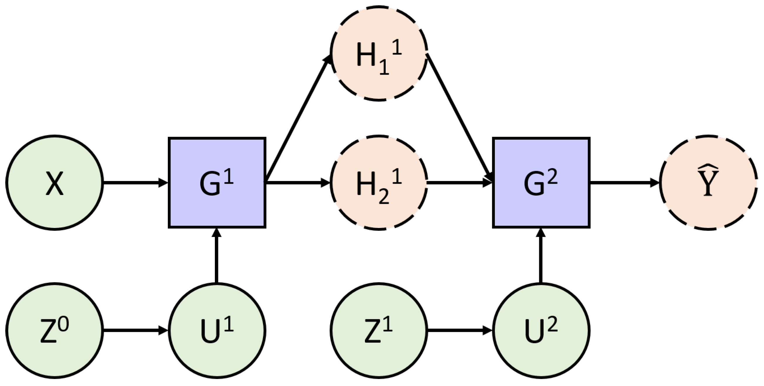
Figure 5 graphically exhibits how the different random variables interact with each other. The straight green circles correspond to variables, which are strictly Gaussian. The dashed orange circles correspond to variables that are not conditionally Gaussian, and the blue rectangles symbolise the conditioning process. In addition, each layer is conditionally independent to the others.

From this additional assumption, the model evidence $f_{\left(\mathbf{Y}\right|{\mathbf{H}}^0)}$ can be written as Equation (15) and similarly to the GP, it is optimised to obtain optimal values for the parameters.

$$\begin{array}{cc}\hfill log\left(f_{\left(\mathbf{Y}\right|{\mathbf{H}}^0)}\left(y\right)\right)& \hfill =log\left({\int }_{{\mathbf{U}}^{\ell }}{\int }_{{\mathbf{H}}^{\ell }}{f}_{(\mathbf{Y},{\mathbf{H}}^{\ell },{\mathbf{U}}^{\ell }|{\mathbf{H}}^0)}(y,h^{\ell },u^{\ell }|h^0)d{\mathbf{H}}^{\ell }d{\mathbf{U}}^{\ell }\right)\hfill \\ \hfill & \hfill =log\left({\int }_{{\mathbf{U}}^{\ell }}{\int }_{{\mathbf{H}}^{\ell }}{f}_{\left(\mathbf{Y}\right|{\mathbf{H}}^L)}{f}_{\left({\mathbf{H}}^{\ell }\right|{\mathbf{H}}^{\ell -1},{\mathbf{U}}^{\ell })}{f}_{\left({\mathbf{U}}^{\ell }\right)}d{\mathbf{H}}^{\ell }d{\mathbf{U}}^{\ell }\right)\hfill \end{array}$$

(15)

where ${\mathbf{H}}^{\ell }:={\left\{{\mathbf{H}}_{\ell }\right\}}_{\ell =1}^L$, ${\mathbf{U}}^{\ell }={\left\{{\mathbf{U}}_{\ell }\right\}}_{\ell =1}^L$, ${\int }_{{\mathbf{H}}^{\ell }}:={\int }_{{\mathbf{H}}^L}\cdots {\int }_{{\mathbf{H}}^1}$, ${\int }_{{\mathbf{U}}^{\ell }}:={\int }_{{\mathbf{U}}^L}\cdots {\int }_{{\mathbf{U}}^1}$ and ${\displaystyle f_{\left({\mathbf{H}}^{\ell }\right|{\mathbf{H}}^{\ell -1},{\mathbf{U}}^{\ell })}{f}_{\left({\mathbf{U}}^{\ell }\right)}:=\prod _{\ell =1}^L{f}_{\left({\mathbf{H}}_{\ell }^{}\right|{\mathbf{H}}_{\ell -1}^{},{\mathbf{U}}_{\ell }^{})}{f}_{\left({\mathbf{U}}_{\ell }^{}\right)}}$.

This model evidence can be decomposed into two parts. The first member of the integrand $f_{\left(\mathbf{Y}\right|{\mathbf{H}}^L)}$ corresponds to the likelihood of the data. The second member $f_{\left({\mathbf{H}}^{\ell }\right|{\mathbf{H}}^{\ell -1},{\mathbf{U}}^{\ell })}{f}_{\left({\mathbf{U}}^{\ell }\right)}$ is the DGP prior. Unfortunately, this prior is not analytically tractable due to the successive inversion of the covariance matrix $\mathbf{C}({\mathbf{H}}^{\ell -1},{\mathbf{H}}^{\ell -1})$ which prevents the computation of the conditional density function $f_{\left({\mathbf{H}}^{\ell }\right|{\mathbf{H}}^{\ell -1},{\mathbf{U}}^{\ell })}$.

Following a variational inference approach, the variational distribution $q_{({\mathbf{H}}^{\ell },{\mathbf{U}}^{\ell })}$, reminded in Equation (16), is introduced to remove this issue of tractability. The representativeness of the distribution is maintained over the conditional density function $f_{\left({\mathbf{H}}^{\ell }\right|{\mathbf{H}}^{\ell -1},{\mathbf{U}}^{\ell })}$ and the approximation is carried out on the inducing variables.

$${\displaystyle q_{({\mathbf{H}}^{\ell },{\mathbf{U}}^{\ell })}=\prod _{\ell =1}^L{f}_{\left({\mathbf{H}}^{\ell }\right|{\mathbf{U}}^{\ell },{\mathbf{H}}^{\ell -1})}{q}_{\left({\mathbf{U}}^{\ell }\right)}}$$

(16)

where $q_{\left({\mathbf{U}}^{\ell }\right)}$ is the variational distribution of ${\mathbf{U}}^{\ell }$ and is Gaussian distributed with ${\left({\mathbf{U}}^{\ell }\right)}_q\sim \mathcal{N}({\mathbf{m}}^{\ell },{\mathbf{S}}^{\ell })$. The subscript q refers to the variational nature of the distribution describing the random variable. ${\mathbf{m}}^{\ell }$ and ${\mathbf{S}}^{\ell }$ are the mean and the variance of ${\mathbf{U}}^{\ell }$.

The inducing variables can be marginalised to obtain the variational distribution of ${\mathbf{H}}^{\ell }$, which is still Gaussian distributed with the mean given by Equation (17) and the variance given by Equation (18).

$$\begin{array}{cc}\hfill \widetilde{{\mu }^{\ell }}& \hfill =\mu \left({\mathbf{H}}^{\ell -1}\right)+\mathbf{A}({\mathbf{m}}^{\ell }-\mu \left({\mathbf{Z}}^{\ell }\right))\hfill \end{array}$$

(17)

$$\begin{array}{cc}\hfill \widetilde{{\Sigma }^{\ell }}& \hfill ={\mathbf{C}}_{HH}-\mathbf{A}({\mathbf{C}}_{ZZ}-{\mathbf{S}}^{\ell }){\mathbf{A}}^T\hfill \end{array}$$

(18)

where $\mathbf{A}={\mathbf{C}}_{HZ}{\mathbf{C}}_{ZZ}^{-1}$, ${\mathbf{C}}_{HZ}=\mathbf{C}({\mathbf{H}}^{\ell -1},{\mathbf{Z}}^{\ell -1})$, ${\mathbf{C}}_{ZZ}=\mathbf{C}({\mathbf{Z}}^{\ell -1},{\mathbf{Z}}^{\ell -1})$ and ${\mathbf{C}}_{HH}=\mathbf{C}({\mathbf{H}}^{\ell -1},{\mathbf{H}}^{\ell -1})$

Thus, due to the conditional dependence of each layer given the previous layer, the computation of a realisation of the density function $\left({\mathbf{H}}^L\right)$ is carried out by propagating the given input x through each layer.

Combining the Equation (16) with the Equation (15) gives the logarithmic mathematical expectation of the model evidence over the variational distribution of inducing variables (Equation (19)).

$$\begin{array}{cc}\hfill log\left(f_{\left(\mathbf{Y}\right|{\mathbf{H}}^0)}\left(y\right)\right)& =log\left({\int }_{{\mathbf{U}}^{\ell }}{\int }_{{\mathbf{H}}^{\ell }}{f}_{\left(\mathbf{Y}\right|{\mathbf{H}}^L)}{f}_{\left({\mathbf{H}}^{\ell }\right|{\mathbf{H}}^{\ell -1},{\mathbf{U}}^{\ell })}{f}_{\left({\mathbf{U}}^{\ell }\right)}\frac{q_{({\mathbf{H}}^{\ell },{\mathbf{U}}^{\ell })}}{q_{({\mathbf{H}}^{\ell },{\mathbf{U}}^{\ell })}}d{\mathbf{H}}^{\ell }d{\mathbf{U}}^{\ell }\right)\hfill \\ \hfill & =log\left({\int }_{{\mathbf{U}}^{\ell }}{\int }_{{\mathbf{H}}^{\ell }}{q}_{({\mathbf{H}}^{\ell },{\mathbf{U}}^{\ell })}{f}_{\left(\mathbf{Y}\right|{\mathbf{H}}^L)}\frac{f_{\left({\mathbf{U}}^{\ell }\right)}}{q_{\left({\mathbf{U}}^{\ell }\right)}}d{\mathbf{H}}^{\ell }d{\mathbf{U}}^{\ell }\right)\hfill \\ \hfill & =log\left({\mathbb{E}}_{{({\mathbf{H}}^{\ell },{\mathbf{U}}^{\ell })}_q}\left[f_{\left(\mathbf{Y}\right|{\mathbf{H}}^L)}\frac{f_{\left({\mathbf{U}}^{\ell }\right)}}{q_{\left({\mathbf{U}}^{\ell }\right)}}\right]\right)\hfill \end{array}$$

(19)

Since the logarithmic function is a concave function, the Jensen’s inequality [40] can be used to obtain a lower bound of the model evidence.

$$\begin{array}{cc}\hfill log\left(f_{\left(\mathbf{Y}\right|{\mathbf{H}}^0)}\left(y\right)\right)& \ge {\mathbb{E}}_{{({\mathbf{H}}^{\ell },{\mathbf{U}}^{\ell })}_q}\left[log\left(f_{\left(\mathbf{Y}\right|{\mathbf{H}}^L)}\frac{f_{\left({\mathbf{U}}^{\ell }\right)}}{q_{\left({\mathbf{U}}^{\ell }\right)}}\right)\right]\hfill \\ \hfill & \ge {\mathbb{E}}_{{({\mathbf{H}}^{\ell },{\mathbf{U}}^{\ell })}_q}\left[log\left(f_{\left(\mathbf{Y}\right|{\mathbf{H}}^L)}\right)\right]+{\mathbb{E}}_{{({\mathbf{H}}^{\ell },{\mathbf{U}}^{\ell })}_q}\left[log\left(\frac{f_{\left({\mathbf{U}}^{\ell }\right)}}{q_{\left({\mathbf{U}}^{\ell }\right)}}\right)\right]\hfill \\ \hfill & \ge {\mathbb{E}}_{{\left({\mathbf{H}}^L\right)}_q}\left[log\left(f_{\left(\mathbf{Y}\right|{\mathbf{H}}^L)}\right)\right]+{\mathbb{E}}_{{\left({\mathbf{U}}^{\ell }\right)}_q}\left[log\left(\frac{f_{\left({\mathbf{U}}^{\ell }\right)}}{q_{\left({\mathbf{U}}^{\ell }\right)}}\right)\right]\hfill \\ \hfill & {\displaystyle \ge {\mathbb{E}}_{{\left({\mathbf{H}}^L\right)}_q}\left[log\left(f_{\left(\mathbf{Y}\right|{\mathbf{H}}^L)}\right)\right]-\sum _{\ell =1}^p{D}_{KL}\left(q_{\left({\mathbf{U}}^{\ell }\right)}\left|\right|f_{\left({\mathbf{U}}^{\ell }\right)}\right)}\hfill \end{array}$$

(20)

where $D_{KL}$ is the Kullback–Leibler divergence between the variational and the true distribution of ${\mathbf{U}}^{\ell }$.

The lower bound given by the Equation (20) is called the efficient lower bound (hereby denoted ELBO) and provides a tight bound for the model evidence. The Kullback–Leibler divergence is in closed form since both distributions are Gaussian distributed. Nevertheless, the tractability of the first term is dependent on the type of likelihood chosen. Indeed, for the Gaussian and Poisson likelihood, this term can be determined analytically. Otherwise, a Gaussian quadrature or a Monte Carlo sampling can be used. For either case, the computation of the first term is done by propagating each instance into the surrogate model.

Considering the expectation of the likelihood given the variational distribution, the first ELBO term becomes (Equation (21)) since each sample from the training set $\mathcal{T}$ is independent.

$${\mathbb{E}}_{{\left({\mathbf{H}}^L\right)}_q}\left[log\left(f_{\left(\mathbf{Y}\right|{\mathbf{H}}^L)}\right)\right]={\mathbb{E}}_{{\left({\mathbf{U}}_s^L\right)}_q}\left[log\left(f_{\left(y_s\right|{\mathbf{H}}_s^L)}\right)\right]$$

(21)

where ${\left({\mathbf{U}}_s^L\right)}_q$ is a realisation of the variational distribution of ${\mathbf{U}}^L$ for the sample ${\mathbf{x}}_s$; $y_s$ is the image of ${\mathbf{x}}_s$ through the function f; and ${\left({\mathbf{H}}_s^L\right)}_q$ is a realisation of the distribution of ${\mathbf{H}}^L$ for the sample ${\mathbf{x}}_s$.

In addition, the re-parameterisation trick, introduced by Rezende et al. [41] and Kingma et al. [42], in the context of Bayesian inference, is considered and given by Equation (22). This trick allows a better optimisation of variational distributions.

$${\mathbf{H}}_s^{\ell }=\tilde{\mu }\left({\mathbf{H}}_s^{\ell -1}\right)+{ϵ}_s^{\ell }\sqrt{\tilde{\Sigma }({\mathbf{H}}_s^{\ell -1},{\mathbf{H}}_s^{\ell -1})}$$

(22)

where ${ϵ}_s^{\ell }$ is a Gaussian-distributed random variable given by $\left({ϵ}_s^{\ell }\right)\sim \mathcal{N}(0,\mathbf{I})$ with $\mathbf{I}$ being the identity matrix.

Considering this trick and the Equation (21), the ELBO reduces to (Equation (23)).

$${\displaystyle \mathrm{ELBO}={\mathbb{E}}_{\left({ϵ}_s^L\right)}\left[log\left(f_{\left(y_s\right|{\mathbf{H}}_s^L)}\right)\right]-\sum _{\ell =1}^L{D}_{KL}\left(q_{\left({\mathbf{U}}^{\ell }\right)}\left|\right|f_{\left({\mathbf{U}}^{\ell }\right)}\right)}$$

(23)

where ${\mathbf{H}}_s^L$ is determined with the Equation (22). The analytical forms for both terms are given in (Equations (A1) and (A2)) from the Appendices Appendix A and Appendix B.

Once the parameters are optimised, the prediction is done by propagating vectors x${}_{*}$ through the surrogate model with the Equation (24). Since $\left({\mathbf{H}}^L\right)$ is not Gaussian distributed and depends on the ${ϵ}_s^{\ell }$ random variable, T samples are drawn from its distribution and then averaged.

$${\displaystyle q_{\left({\mathbf{H}}_{*}^L\right)}=\frac{1}{T}\sum _{t=1}^T{q}_{\left({\mathbf{H}}_t^L\right)}}$$

(24)

where $q_{\left({\mathbf{H}}_t^L\right)}$ is the tth realisation of the variational distribution of $\left({\mathbf{H}}^L\right)$.

Table 6. DGP parameters and hyperparameters.

Name of the Quantity	Nature of the Quantity	Associated Variable	Equation
Hidden layer number	Hyperparameter	p	Equation (12)
Neuron number	Hyperparameter	$D^{(\ell )}$	Equation (7)
Pseudo-inputs number	Hyperparameter	m	Equation (14)
Kernel	Hyperparameter	$\mathbf{K}$	Table 2
Likelihood	Hyperparameter	$f_{\left(\mathbf{Y}\right|{\mathbf{H}}^L)}$	Equation (15)
Lengthscale	Parameter (Deterministic)	${\mathsf{\Theta }}^{\ell }$	Equation (7)
Pseudo-inputs locations	Parameter (Deterministic)	$Z^{\ell }$	Equation (14)
Signal variance	Hyperparameter	${\sigma }_k^{2,\ell }$	Equation (7)
Data noise	Hyperparameter	${\sigma }_n^2$	Equation (A1)
Mean function	Hyperparameter	${\mu }^{\ell }$	Equation (17)
Variational mean	Parameter (Variational)	${\mathbf{m}}^{\ell }$	Equation (16)
Variational covariance matrix	Parameter (Variational)	${\mathbf{S}}^{\ell }$	Equation (16)

summarises the different quantities considered in the DGP surrogate model. The hyperparameters and parameters in italics are repeated for each layer. The signal variance and data noise are fixed, invoking the same reasons as for the GP.

4. Analysis of the Performance of the Surrogate for a One Dimensional Problem

4.1. Preamble

The aim of this section is to evaluate the performance of the surrogate models presented in Section 3, when considering the approximation of the four complex eigenvalues of the Double Hulten. To do so, the effects of the hyperparameter setting are thoroughly studied.

The most challenging one dimensional configuration is considered by taking the friction coefficient as an input variable. This parameter generates non-linear behaviours and asymmetries in the contact matrices and is, thus, the most complex parameter to manage.

Finally, for engineering applications, small training sets (about 200 to 300 samples, maximum) are mandatory to maintain the computational cost compliant with industrial process. Hence, the number of samples used to train the surrogate models is reduced following this limitation. The samples number is parameterised with regard to the number of dimension to give a reference for the comparison of scenarios with different number of dimensions.

4.1.1. Toolboxes and Hyperparameter Setting

The current applications are based on different Python toolboxes. The GP model is constructed with the GPFlow toolbox [43], and its parameters are optimised using the LBFGS algorithm [38]. Next, the DGP model is generated with the doubly stochastic toolbox [25], and its deterministic parameters, namely the location of the pseudo-points and the lengthscales of the kernel of each layer, are optimised using Adam [44]. With regard to the variational parameters, namely the mean and variance matrix of each layer, they are optimised using the natural gradient descent method, introduced by Salimbeni et al. [45]. For the DNN, the Scikit-Learn toolbox [46] is used, and the optimisation is carried out with the LBFGS algorithm.

Some of the hyperparameters, shown in Table 3, Table 5 and Table 6, are put aside in this sequel and are not studied based on the following reasons. Since the solver is exact and the data are standardised, there is no need to optimise the data noise and signal variance with respect to the loss function. Following Ginsbourger’s conclusions [47], for the GP and the DGP, the mean function is not considered and taken to be a zero function. As for the number of DGP pseudo-inputs, Salimbeni’s formalism [25] does not allow inferring an optimal number, but rather to impose a user selection of this number. Concerning the likelihood, it is also user defined and carries the hypothesis on the relationship between the output and the realisation of the DGP. Finally, for the DNN, the regularisation is traditionally set to 0.0001 [46].

Table 7. Fixed hyperparameters for the GP, the DNN and the DGP.

Surrogate Model	Hyperparameter Name	Symbol	Equations	Value
GP	Signal variance	${\sigma }_{\mathrm{k}}^2$	Equation (7)	1
GP	Data noise	${\sigma }_{\mathrm{n}}^2$	Equation (5)	${10}^{-6}$
GP	Mean function	$\mu$	Equation (5)	Zero ()
DNN	Regularisation	$\alpha$	Equation (10)	0.0001
DGP	Pseudo-inputs number	m	Equation (14)	n
DGP	Likelihood	$f_{\left(\mathbf{Y}\right|{\mathbf{H}}^L)}$	Equation (15)	Gaussian
DGP	Signal variance	${\sigma }_k^{\ell }$	Equation (7)	1
DGP	Data noise	${\sigma }_n^2$	Equation (A1)	${10}^{-3}$
DGP	Mean function	${\mu }^{\ell }$	Equation (17)	Zero ()

summarises the fixed hyperparameters of the study with their associated values.

Similarly, the parameters of the optimisers are given in

Table 8. Optimisation parameters for the DGP.

Optimiser	Name	Value
Adam	Step	${10}^{-3}$
	Learning rate (Alpha)	0.8
	First moment decay rate (Beta)	0.8
	Epsilon	${10}^{-8}$
Natural Gradient	Step	${10}^{-3}$

.

4.1.2. Experimental Protocol

The approximated functions are given in Section 2.1 and correspond to the real and imaginary parts of the four eigenvalues of the Double Hulten. As mentioned earlier, the friction coefficient is considered variable, while the other parameters are fixed, following the values of Table 7. Ten randomly distributed training sets are generated for three different sizes: 6, 10 and 15 samples per dimension, using an LHS.

Considering the surrogate model definition and the remaining hyperparameters (

Table 9. Studied hyperparameters for the three surrogate models.

Surrogate	Kernel/Activation Function	Hidden Layers	Neurons
GP	RBF, Matern 3/2 (M32), Matern 5/2 (M52)	-	-
DNN	ReLU, Tanh, Logistic	$[1,4]$	{50,100,150,200,250,300}
DGP	Matern 3/2 (M32), Matern 5/2 (M52)	$[1,4]$	1-3-7-10

), several values are tested to evaluate the performance of each surrogate model depending on its setting and the number of samples used for training.

For the GP, only the kernel is taken into account here. For the DGP and DNN, the deep nature of these surrogate models requires a more complex architecture than the one of the GP. Thus, a parametric study of the definition of hidden layers and associated neurons per layer is carried out in addition to the analysis of the kernel/activation functions. The RBF function is put aside for the DGP due to the non convincing results. The DGP architecture values were chosen with regard to the literature [25,30], and the DNN was set according to many tests.

For the GP and DGP, the lengthscale is initialised at a value of 1, while the weight of the DNN is randomly initialised. These quantities are then optimised, considering the optimisation algorithms, presented in Section 4.1.1.

As the purpose is here to assess the surrogate performance over the entire model, the whole spectrum is considered. Nonetheless, each real and imaginary parts of the eigenvalue is assumed to be independent, inducing one surrogate training per quantity of interest. A CRMSE criterion, given by Equation (25), is used to account for the whole spectrum approximation capabilities. To validate our different predictions, a validation set of 10,000 values is defined.

$$\mathrm{CRMSE}=\sqrt{\frac{{\displaystyle \sum _{j=1}^t\sum _{i=1}^{n_{\mathrm{test}}}{\left(y_{ij}-{\widehat{y}}_{ij}\right)}^2}}{t\times n_{\mathrm{test}}}}$$

(25)

where $n_{\mathrm{test}}$ is the number of test values, and t is the number of considered eigenvalues to approximate. Then, $y_{ij}$ and ${\widehat{y}}_{ij}$ are the reference and the surrogate approximation values for the ith sample of the jth eigenvalue.

4.2. Best Hyperparameter Setting for Small Training Sets

4.2.1. Performance Overview

Figure 6 presents the CRMSE range of variation for the ten randomly distributed training sets—the min-max bounds are given with squares, while the mean performance over the training sets is displayed with a circle. In addition, the results considering the sample density (6, 10 and 15 samples) are respectively shown in red, blue and black interval performance. For all the tested hyperparameter settings, the CRMSE value is compared, and the configurations associated with the lowest CRMSE value are denoted as the best configuration. This analysis is carried out on the averaged CRMSE over the training set.

The real and imaginary approximation performance are displayed on the left and right sides of each figure. Finally, a colour map is added in the background to denote the interpretation of the CRMSE: a CRMSE value greater than 1 is associated with a bad performance, while a CRMSE value lower than 0.5 is linked to a good performance. Between these two bounds, the results are mitigated and cannot be considered efficient nor bad.

Observations

First, considering the best hyperparameter setting, the best surrogate model is clearly the DNN: whatever the training set size, the mean performance over the 10 training sets is associated with a good CRMSE for the real part approximation, or at least a mitigated CRMSE (6 samples) and then a good CRMSE (10 to 15 samples) for the imaginary part.

With regard to the DGP, the overall performance is slightly better than for the GP. Indeed, for 6 samples, both surrogate models almost perform identically. For the approximation of the real parts with 10 samples, the DGP provides a better approximation since both the mean and maximum CRMSE are linked to a good CRMSE value (respectively, 0.35 and 0.48). Conversely, the GP slightly performs worse by providing a mean CRMSE of 0.61 and a maximum CRMSE of roughly 1. For other scenarios, the results differ little.

Finally, the real part approximations are more sensitive to the sample distribution, especially for the GP and the DNN. Indeed, the min-max bounds of the first surrogate roughly spread about 0.3 CRMSE points, while the latter bounds spread about 0.6. Conversely, the DGP allows more stable approximations since the bounds spreads are roughly 0.1 CRMSE points.

Table 10. Best hyperparameter setting of GP, DGP and DNN.

Surrogate Model	Training Set Size	6 Points		10 Points		15 Points
	Approximated Function	Real	Imag.	Real	Imag.	Real	Imag.
GP	Kernel	M32	M32	M52	M32	M32	M32
DGP	Kernel	M32	M32	M32	M32	M32	M32
	Architecture	(4,10)	(2,10)	(2,7)	(3,7)	(2,10)	(1,10)
DNN	Activation function	ReLU	ReLU	ReLU	Tanh	Tanh	Tanh
	Architecture	(4,150)	-	(4,300)	-	-	-

exhibits the hyperparameter settings that led to the mean CRMSE, shown in Figure 6. These best settings are determined by taking the mean trend of the surrogate model performance over all the considered training sets. Typically, a hyphen is put for surrogate models, where no particular mean trend can be emphasised, highlighting the instability of the given surrogate model toward its hyperparameter setting. Moreover, for the DNN and the DGP, the values in the brackets give the number of hidden layers and neurons. The bold text of Table 10 highlights the following observations about the best hyperparameter setting.

The GP and DGP exhibits the highest performance when the Matern 3/2 is used, whatever the considered approximated functions. For the architecture of the DGP, the best hyperparameter setting is almost always associated with a medium deep structure. Finally, for the DNN, the results are rather mitigated. Indeed, the performance for the small density sample distribution (real and imaginary approximation) and the medium density sample distribution is maximised when the ReLU activation function is considered; however, for the other considered scenarios, the Tanh is needed. In addition, no particular trend has been highlighted for the imaginary approximation with regard to the hidden layer and neuron settings of the DNN.

Discussions

The results of the kernel functions are, in a way, relevant to the mathematical properties of these functions. Indeed, Matern 3/2 is only once differentiable, making it highly rough. The roughness of this function allows the surrogate model to deal with higher non-linearities than the RBF, which is infinitely differentiable and therefore highly smooth. This property is, thus, highly interesting while dealing with friction-induced vibration problems, due to the non-linearities involved in the models.

For the DNN, the hyperparameter setting instability is one of the main flaws of this surrogate model. Indeed, this issue enforces the user to evaluate numerous configurations to find the best one. As a result, no conclusion can be drawn toward the hyperparameter setting of this surrogate. Piotrowski et al. [48] tried to tackle this issue, but it is still open research.

4.2.2. Sample Distribution Density Effect

Figure 7 proposes an assessment of the approximation quality with respect to the sample distribution density for a given training set. The first row of Figure 7a–c corresponds to the approximation with 6 samples; the second row of Figure 7d–f, with 10 samples; and the final row of Figure 7g–i, with 15 samples. The hyperparameters used for training the surrogate models are given in Table 10.

First, whatever the training set size, the prediction of each surrogate model is merely identical, except for the 10 samples (Figure 7d–f) where the approximations are slightly different for a friction coefficient between 0.8 and 1.

Moreover, as the use of a 6 sample training set allows a coarse prediction of the behaviour of the considered function, a 10 sample training set gives a rather good approximation. The 15 samples training set generates a perfect prediction, but the additional computation cost for computing the 5 additional samples is not justified, considering the given increase in accuracy.

Table 11. CRMSE values with respect to the sampling density for each surrogate model.

Number of Samples	Gaussian Process	Deep Gaussian Process	Deep Neural Network
6 samples	0.91	0.518	0.666
10 samples	0.57	0.357	0.206
15 samples	0.119	0.113	0.128

shows the CRMSE values for the configurations considered in Figure 7. The previous observations are confirmed by the numerical values of the CRMSE, namely that, for 15 samples, each surrogate model provides the same level of performance, and that, for 10 samples, the approximation is fair enough for any surrogate model.

4.3. Worst Hyperparameter Setting for Small Training Sets

4.3.1. Performance Overview

Figure 8 presents the CRMSE range of variation for the ten randomly distributed training sets in a similar way than for the best hyperparameter setting. For all the tested hyperparameter settings, the CRMSE value is compared, and the configurations associated with the highest CRMSE value is denoted as the worst configuration. This analysis is carried out on the averaged CRMSE over the training set.

Observations

First, for the DGP and the DNN, the real-part approximations are clearly acceptable when the number of samples is greater than 10 points, even with a bad hyperparameter setting. Indeed, for the DNN, the worst performance of the mean approximation of the real part is always associated with a good CRMSE value. Conversely, for the DGP, it is at least linked to a mitigated CRMSE value.

However, for the GP approximation, the results are more problematic. Indeed, for the first surrogate model, the CRMSE range of variation is wider for a sample number of 15 than for the smaller training set sizes. For instance, the range of variations is respectively about 1 CRMSE point and 3 CRMSE points for the approximations of the real and imaginary parts. With regard to the DNN imaginary part approximations, the results are also problematic, whatever the training set size. The CRMSE is even greater than 10 for 6 training samples.

Table 12. Worst hyperparameter setting of GP, DGP and DNN.

Surrogate Model	Training Set Size	6 Points		10 Points		15 Points
	Approximated function	Real	Imag.	Real	Imag.	Real	Imag.
GP	Kernel	RBF	RBF	RBF	RBF	RBF	RBF
DGP	Kernel function	M52	M52	M52	M52	M52	M52
	Architecture	(3,10)	(4,10)	(3,10)	(4,10)	(4,10)	(4,10)
DNN	Activation function	TanH	ReLU	Logistic	ReLU	Logistic	ReLU
	Architecture	(4,200)	(4,300)	-	(4,200)	-	(4,200)

shows the hyperparameter settings that led to the mean CRMSE, shown in Figure 8. The procedure is similar to the one explained for Table 10.

The worst GP and DGP settings are stable with regard to the kernel function. Whatever the considered approximated functions, the RBF (respectively, Matern 5/2) gives the worst results. For the architecture of the DGP and the DNN, deeper structures cause the worst approximations since the worst hyperparameter setting is associated with four hidden layers for both surrogate models. The DNN produces unstable approximation results, especially for the real prediction with 10 and 15 samples, where no particular hyperparameter setting is clearly identified.

Discussions

The instability of the hyperparameter setting of the DNN is highlighted for the worst setting. Here, the ReLU activation function generates bad approximations, especially for the imaginary functions. This can be easily explained by the characteristics of the activation function. Indeed, the ReLU cannot be differentiated due to the use of the maximum operator. Consequently, it is more adapted to highly non-linear approximations. Here, the imaginary functions are the frequencies of the studied problem, which remain relatively smooth, despite the (large) variation of the friction coefficient.

Conversely, the DGP exhibits more stable results than the DNN. The performance for the worst hyperparameter setting is pretty close to the performance with the best setting. For instance, the approximation of the imaginary functions with 10 samples generates an error of 0.42 with the best setting, while an error of 0.5 is generated with the worst setting.

Finally, the observations about the roughness of the kernel functions are still valid here since the smoothest functions (the RBF and the Matern 52) generate the worst approximations, respectively, for the GP and the DGP.

The next section focuses on the two scenarios where the GP and the DNN produce erroneous predictions. The purpose is to highlight the consequence of the issue of both surrogate models over their approximation capabilities and to compare with the DGP approximation.

4.3.2. Erroneous Predictions for GP and DNN

Figure 9 focuses on a limitation of the GP surrogate model for specific training sets. The GP prediction Figure 9a is constant on the majority of the design space, except at the vicinity of the samples of the training sets. Hence, this deceptive approximation clearly affects the predictivity of the surrogate model, yielding it unusable in this case. However, when a deep architecture is taken into account, this problem of deceptive approximation does not appear. For both other surrogate models, the prediction is almost perfect.

Similarly, Figure 10 highlights a limitation of the DNN surrogate model that appears with six samples, but can appear whatever the considered training set. Whereas GP and DGP approximation are almost similar and quite efficient with regard to the training set information, the DNN does not give a good approximation at all. Indeed, between each sample, the prediction is highly fractured.

This phenomenon is called overfitting and was first emphasised by Runge [37]. In a nutshell, overfitting corresponds to the case when the surrogate model becomes very efficient to explain the training set, but cannot explain other set of samples (namely the test set). Consequently, the prediction oscillates quickly, and the surrogate model is unusable. This issue is known to be frequent with the neural network [35,49]. This is still an open research field, although many methods have been proposed to overcome this phenomenon [48].

4.4. Conclusions

This section shows that, considering an optimal hyperparameter setting, the approximations provided by the surrogate models are interchangeable and any of them can be used. In addition, the optimal sample density is showed to be 10 samples per dimension since it allows a good representation of the design space, while limiting the computational cost.

For the hyperparameter setting, the GP and the DGP were showed to be pretty stable. Indeed, for both surrogate models, Matern 3/2 corresponds to the best kernel function. For the DGP, a mid-deep structure gave the most efficient approximations. For the DNN, the results were more mitigated. Indeed, no clear conclusions were drawn from these results, and a good hyperparameter setting for a given training set can become a bad setting for another sample distribution. This enforces the user to evaluate a lot of configurations to find the most efficient one.

Consequently, the DNN is set aside due to its instability with respect to the hyperparameter setting, whatever the number of samples in the training set and the quantity to approximate. In addition, the DNN does not provide a direct measure of the modelling uncertainty (the variance of GP and DGP), which is a critical issue in Bayesian optimisation, for instance [50]. It is possible to obtain a substitute to the variance when using the DNN, but the implementation is more complex.

5. Applications of Gaussian Processes and Deep Gaussian Processes in a Multiparametric Analysis

5.1. Hyperparameter Setting of the Deep Gaussian Process in a Multiparameteric Analysis

5.1.1. Preamble

This section aims at highlighting the evolution of the DGP performance with respect to the dimensionality of the problem. Many tests showed that, unlike the GP, the hyperparameter setting conclusions on the 1-dimensional problem do not extend to n-dimensional problems. Thus, a discussion on the optimal architecture of the DGP is given to emphasise the relation between the system parameters and the capacity of the DGP to efficiently approximate the whole frequency spectrum.

To do so, the analysis is decomposed into two steps: first, the approximation of the eigenvalues of the Double Hulten model is considered with five variable parameters. Then, three scenarios are studied with three, five and seven variable parameters.

5.1.2. Five-Dimensional Study

The following parameters of the Double Hulten are considered variable: $m_1$, $m_2$, $k_a$, $c_a$ and $\mu$, with a variation of ±10%, except for the friction coefficient, which varies between 0 and 1. The first four parameters are similar to the structural parameters of a real brake system. With regard to the training set $\mathcal{T}$, used to train the surrogate model, 10 sets, composed of 50 samples (10 per parameter) are randomly generated using an LHS. A DGP is built for different hidden layers and neurons setting.

Observations

Table 13. CRMSE for real part approximations.

Neurons	Hidden Layers
	1	2	3	4
1	6.29	6.13	6.23	6.29
3	4.35	4.33	4.32	4.32
5	0.468	0.469	0.47	0.47
7	0.467	0.469	0.478	0.478
10	0.467	0.468	0.491	0.489

and

Table 14. CRMSE for imaginary part approximations.

Neurons	Hidden Layers
	1	2	3	4
1	6.29	6.13	6.23	6.29
3	4.35	4.33	4.32	4.32
5	0.468	0.469	0.47	0.47
7	0.467	0.469	0.478	0.478
10	0.467	0.468	0.491	0.489

show the CRMSE values for the DGP prediction over a MC sampling of 10,000 reference samples. The values for the hidden layers and neurons setting are given in these tables.

First, two levels of performance are highlighted in these tables. The DGP provides bad approximations when the number of neurons is lower or equal to 3. Conversely, when the number of neurons is at least equal to 5, the approximations are efficient for both real and imaginary parts of the eigenvalues.

Secondly, the performance is quite stable over the number of neurons and the number of hidden layers, with a CRMSE around 0.47 for the real part and around 0.45 for the imaginary part. Thus, one hidden layer is sufficient to provide efficient approximations.

From the analysis of the previous results, the number of neurons has to be at least set to 5, which corresponds to the number of parameters taken into account, for either the real or the imaginary part approximations. To validate this assertion, the following section focuses on the study of scenarios which involve several variable parameters.

5.1.3. N-Dimensional Study

The three considered scenarios are the following ones:

• 3 input parameters: $m_1$, $m_2$ and $\mu$;
• 5 input parameters: $m_1$, $m_2$, $k_a$, $c_a$ and $\mu$;
• 7 input parameters: $k_{11}$, $k_{12}$, $k_{21}$, $k_{22}$, $k_a$, $c_a$, and $\mu$.

Similar to the previous test, for the performance evaluation, 10 training sets are randomly generated with 10 samples per input parameter (30, 50 and 70 samples on overall for each scenario).

Observations

The CRMSE values for each configuration and each scenario are given in

Table 15. CRMSE for real part approximations with 3D, 5D and 7D scenarios.

3D		5D		7D
Neurons	CRMSE	Neurons	CRMSE	Neurons	CRMSE
1	6.355	1	6.29	1	6.219
2	4.349	3	4.35	3	5.319
3	0.491	5	0.468	5	4.722
4	0.491	7	0.467	7	0.541
5	0.491	10	0.467	10	0.541

and

Table 16. CRMSE for imaginary part approximations with 3D, 5D and 7D scenarios.

3D		5D		7D
Neurons	CRMSE	Neurons	CRMSE	Neurons	CRMSE
1	6.079	1	6.159	1	5.876
2	3.915	3	4.266	3	4.969
3	0.471	5	0.448	5	4.101
4	0.471	7	0.448	7	0.537
5	0.471	10	0.448	10	0.538

. The assertion of the previous section is validated by those results since, for the 3D scenario, the number of neurons has to be at least 3, and, for the 7D scenario, it should at least be 7.

Discussions

This observation has a strong implication: the formalism of the DGP used in this research is not capable of doing dimension reduction. This limitation of the considered DGP allows stating a rule of thumb about the setting of the DGP: the number of neurons has to be at least equal to the number of parameters.

Moreover, taking a number of neurons greater than the number of parameters also yields efficient results, but, due to the stability of the DGP, its performance is not improved. In the studied applications, one hidden layer provides good performance for the surrogate model approximations. It limits the computational cost induced by the inference of deeper and deeper models.

5.2. Comparison between GP and DGP Performance

This section compares the prediction of the GP using the best hyperparameter setting, highlighted in Section 4.2 and Section 5.1. To do so, the same experimental procedure than the one of the previous section is used, meaning 10 randomly generated training sets with 10 points per dimension, for three scenarios: 3, 5 and 7 parameters.

Observations

Table 17. Comparison between the GP and DGP CRMSE for real and imaginary part approximations with 3D, 5D and 7D scenarios.

Function Type	GP			DGP
	3D	5D	7D	3D	5D	7D
Real	0.53	0.479	0.56	0.491	0.468	0.541
Imag.	0.51	0.464	0.55	0.471	0.448	0.537

shows the CRMSE value for each surrogate approximation. The DGP performs better than the GP, whatever the considered scenario or the approximated quantity (real or imaginary). Nonetheless, the improvements brought by the DGP are small, roughly 0.2 points of CRMSE value.

Discussions

This observation raises some concerns about the relevance of the DGP, used for the approximation of the eigenvalues of an FIV problem. Indeed, all the tests performed in Section 4 and Section 5 proved the efficiency of the DGP; however, the computational cost of training this surrogate model is high. For instance, a GP shows a training time of less than 1 s. The DGP training time is highly dependent on its architecture and the dimensionality of the problem. For these tests, in a one-dimensional problem, the training lasted 2 min to 30 min, on average; for a 5-dimensional problem, the training lasted 2 h to 6 h. Obviously, this training cost can be leveraged by using heavy parallelism, but, because of the accuracy improvement, using the DGP may not be relevant for FIV problems.

Two main reasons can be invoked to justify this weak improvement of accuracy. The first one is that, in the literature, the majority of works on DGP [51,52] use a great amount of samples (from 39 to 5081 samples per dimension in [25], for instance). These training set sizes are not reachable for our kind of application, especially with industrial models, and the DGP may not have sufficient data to be trained.

A second explanation is that the considered functions (the eigenvalues of the squeal problem) are not sufficiently non-linear to highlight a large difference between GP and DGP approximations. Hebbal et al. [30] used the DGP to approximate the constraints of the optimisation problem. Typically, Figure 2a,b clearly shows that the evolution of the real or imaginary part eigenvalues is non-abrupt, even in the coupling areas.

6. Conclusions

In this paper, the performance of the Gaussian process, the deep neural network and the deep Gaussian process were investigated for friction-induced vibration problems subject to variations of mechanical properties. The study aims at illustrating the impact of the surrogate models parameterisation in the case of non-linear and non-stationary evolutions. A focus is mainly made on suboptimal training sets. This suboptimality is a consequence of the use of common random training sets, which need a high sampling density to be fully efficient, non-achievable for traditional engineering applications.

The effects of the most complex parameter of a friction-induced vibration problem, namely the friction coefficient, were studied. Three different training set densities were considered, namely 6, 10 and 15 samples, for 10 randomly distributed training sets. The results showed that, given an optimal hyperparameter setting, all the surrogates are interchangeable. In addition, from a computational cost aspect, the 10 samples per parameter density produces relevant results. The 15 samples density is better, but the small improvement in precision does not counterbalance the increase in the computational cost.

With regard to the hyperparameter setting of the surrogate models, the GP and DGP gave the most efficient results when using the Matern 3/2 kernel function. The performance of the DNN was highly unstable, and no trend was drawn from the results. Many architecture configurations must be evaluated to determine the most suitable one. For specific training sets and non-stationary evolutions, some deceptive predictions were also detected for the Gaussian process. On the other hand, the deep Gaussian process showed an interesting robustness in these situations as soon as rules about the architecture definition were known. The deep Gaussian process is a serious alternative to the GP when the nature of studied behaviours is highly non-stationary, but its main weakness is obviously the computational time when no parallel computations are considered. The results showed that the number of hidden layers and neurons can be controlled to lower the computational cost of the DGP. Indeed, the number of neurons can be set to be equal to the number of uncertain parameters. As for the hidden layer number, it can generally be fixed to one. Finally, a comparison between the GP and the DGP for these multidimensional scenarios was performed. The results showed that the latter one outperforms the first one in term of accuracy. However, the future developments about DGP must be focussed on the reduction in the computational cost to make the method compatible with numerical simulations, currently used in mechanical engineering.

Moreover, a natural extension of this work is to study the deceptive prediction of the Gaussian process. Indeed, the performance of the Gaussian process is quite good for the majority of the considered scenarios, except for specific sample locations. It would be interesting to have a strategy to detect and handle those deceptive predictions. In addition, the use of surrogate modelling is especially interesting when the number of calls to the solver is important. The uncertainty propagation and the optimisation are of those types of application. The use of machine learning techniques was already considered in the literature, but two limitations naturally arise: the curse of dimensionality, which corresponds to an exponential need of samples when the number of parameters increase, and the quality of the approximation, which depends on the representativeness of the randomly evaluated samples. Adaptive sampling strategies could provide an efficient way to tackle these limitations. It would be interesting to investigate these approaches in the case of non-linear functions in the future.

References

1. Kinkaid, N.; O’Reilly, O.; Papadopoulos, P. Automotive disc brake squeal. J. Sound Vib. 2003, 267, 105–166. [Google Scholar] [CrossRef]
2. Massi, F.; Baillet, L.; Giannini, O.; Sestieri, A. Brake squeal: Linear and nonlinear numerical approaches. Mech. Syst. Signal Process. 2007, 21, 2374–2393. [Google Scholar] [CrossRef]
3. Ouyang, H.; Nack, W.; Yuan, Y.; Chen, F. Numerical analysis of automotive disc brake squeal: A review. Int. J. Veh. Noise Vib. 2005, 1, 207. [Google Scholar] [CrossRef]
4. Fritz, G.; Sinou, J.J.; Duffal, J.M.; Jézéquel, L. Effects of damping on brake squeal coalescence patterns—Application on a finite element model. Mech. Res. Commun. 2007, 34, 181–190. [Google Scholar] [CrossRef] [Green Version]
5. Hoffmann, N.; Gaul, L. Effects of damping on mode-coupling instability in friction induced oscillations. ZAMM—J. Appl. Math. Mech./Z. Für Angew. Math. Und Mech. 2003, 83, 524–534. [Google Scholar] [CrossRef]
6. Magnier, V.; Roubin, E.; Colliat, J.; Dufrénoy, P. Methodology of porosity modeling for friction pad: Consequence on squeal. Tribol. Int. 2017, 109, 78–85. [Google Scholar] [CrossRef] [Green Version]
7. AbuBakar, A.R.; Ouyang, H. Wear prediction of friction material and brake squeal using the finite element method. Wear 2008, 264, 1069–1076. [Google Scholar] [CrossRef] [Green Version]
8. Denimal, E.; Sinou, J.J.; Nacivet, S.; Nechak, L. Squeal analysis based on the effect and determination of the most influential contacts between the different components of an automotive brake system. Int. J. Mech. Sci. 2019, 151, 192–213. [Google Scholar] [CrossRef]
9. Graf, M.; Ostermeyer, G.P. Friction-induced vibration and dynamic friction laws: Instability at positive friction–velocity-characteristic. Tribol. Int. 2015, 92, 255–258. [Google Scholar] [CrossRef]
10. Do, H.; Massa, F.; Tison, T.; Lallemand, B. A global strategy for the stability analysis of friction induced vibration problem with parameter variations. Mech. Syst. Signal Process. 2017, 84, 346–364. [Google Scholar] [CrossRef]
11. Lü, H.; Yu, D. Optimization design of a disc brake system with hybrid uncertainties. Adv. Eng. Softw. 2016, 98, 112–122. [Google Scholar] [CrossRef]
12. Tison, T.; Heussaff, A.; Massa, F.; Turpin, I.; Nunes, R. Improvement in the predictivity of squeal simulations: Uncertainty and robustness. J. Sound Vib. 2014, 333, 3394–3412. [Google Scholar] [CrossRef]
13. Sarrouy, E.; Dessombz, O.; Sinou, J.J. Piecewise polynomial chaos expansion with an application to brake squeal of a linear brake system. J. Sound Vib. 2013, 332, 577–594. [Google Scholar] [CrossRef] [Green Version]
14. Massa, F.; Do, H.Q.; Tison, T.; Cazier, O. Uncertain Friction-Induced Vibration Study: Coupling of Fuzzy Logic, Fuzzy Sets, and Interval Theories. ASCE-ASME J. Risk Uncertain. Eng. Syst. Part B Mech. Eng. 2015, 2, 011008. [Google Scholar] [CrossRef]
15. Lü, H.; Cai, Z.; Feng, Q.; Shangguan, W.B.; Yu, D. An improved method for fuzzy–interval uncertainty analysis and its application in brake instability study. Comput. Methods Appl. Mech. Eng. 2018, 342, 142–160. [Google Scholar] [CrossRef]
16. Renault, A.; Massa, F.; Lallemand, B.; Tison, T. Experimental investigations for uncertainty quantification in brake squeal analysis. J. Sound Vib. 2016, 367, 37–55. [Google Scholar] [CrossRef]
17. Massa, F.; Lallemand, B.; Tison, T. Multi-level homotopy perturbation and projection techniques for the reanalysis of quadratic eigenvalue problems: The application of stability analysis. Mech. Syst. Signal Process. 2015, 52–53, 88–104. [Google Scholar] [CrossRef]
18. Sadet, J.; Massa, F.; Tison, T.; Turpin, I.; Lallemand, B.; Talbi, E.G. Homotopy perturbation technique for improving solutions of large quadratic eigenvalue problems: Application to friction-induced vibration. Mech. Syst. Signal Process. 2021, 153, 107492. [Google Scholar] [CrossRef]
19. Brunetti, J.; D’Ambrogio, W.; Fregolent, A. Friction-induced vibrations in the framework of dynamic substructuring. Nonlinear Dyn. 2020, 103, 3301–3314. [Google Scholar] [CrossRef]
20. Monteil, M.; Besset, S.; Sinou, J.J. A double modal synthesis approach for brake squeal prediction. Mech. Syst. Signal Process. 2016, 70–71, 1073–1084. [Google Scholar] [CrossRef]
21. Besset, S.; Sinou, J.J. Modal reduction of brake squeal systems using complex interface modes. Mech. Syst. Signal Process. 2017, 85, 896–911. [Google Scholar] [CrossRef]
22. Denimal, E.; Nechak, L.; Sinou, J.; Nacivet, S. Kriging surrogate models for predicting the complex eigenvalues of mechanical systems subjected to friction-induced vibration. Shock Vib. 2016, 2016, 3586230. [Google Scholar] [CrossRef] [Green Version]
23. Denimal, E.; Sinou, J.J.; Nacivet, S. Influence of structural modifications of automotive brake systems for squeal events with kriging meta-modelling method. J. Sound Vib. 2019, 463, 114938. [Google Scholar] [CrossRef]
24. Talbi, E.G. Automated Design of Deep Neural Networks: A Survey and Unified Taxonomy. ACM Comput. Surv. 2021, 54, 1–37. [Google Scholar] [CrossRef]
25. Salimbeni, H.; Deisenroth, M. Doubly stochastic variational inference for deep gaussian processes. In Proceedings of the Advances in Neural Information Processing Systems, Long Beach, CA, USA, 4–9 December 2017. [Google Scholar]
26. Stender, M.; Tiedemann, M.; Spieler, D.; Schoepflin, D.; Hofffmann, N.; Oberst, S. Deep learning for brake squeal: Vibration detection, characterization and prediction. arXiv 2020, arXiv:2001.01596. [Google Scholar]
27. Kong, Y.; Abdullah, S.; Schramm, D.; Omar, M.; Haris, S. Optimization of spring fatigue life prediction model for vehicle ride using hybrid multi-layer perceptron artificial neural networks. Mech. Syst. Signal Process. 2019, 122, 597–621. [Google Scholar] [CrossRef]
28. Radaideh, M.I.; Kozlowski, T. Surrogate modeling of advanced computer simulations using deep Gaussian processes. Reliab. Eng. Syst. Saf. 2020, 195, 106731. [Google Scholar] [CrossRef]
29. Tagade, P.; Hariharan, K.S.; Ramachandran, S.; Khandelwal, A.; Naha, A.; Kolake, S.M.; Han, S.H. Deep Gaussian process regression for lithium-ion battery health prognosis and degradation mode diagnosis. J. Power Sources 2020, 445, 227281. [Google Scholar] [CrossRef]
30. Hebbal, A.; Brevault, L.; Balesdent, M.; Talbi, E.G.; Melab, N. Bayesian Optimization using Deep Gaussian Processes. arXiv 2019, arXiv:1905.03350. [Google Scholar]
31. Hultén, J. Some Drum Brake Squeal Mechanisms; SAE International: Warrendale, PA, USA, 1995. [Google Scholar] [CrossRef]
32. Gallina, A.; Pichler, L.; Uhl, T. Enhanced meta-modelling technique for analysis of mode crossing, mode veering and mode coalescence in structural dynamics. Mech. Syst. Signal Process. 2011, 25, 2297–2312. [Google Scholar] [CrossRef]
33. Mckay, M.D.; Beckman, R.J.; Conover, W.J. A Comparison of Three Methods for Selecting Values of Input Variables in the Analysis of Output from a Computer Code. Technometrics 2000, 42, 55–61. [Google Scholar] [CrossRef]
34. Rasmussen, C.E.; Williams, C.K.I. Gaussian Processes for Machine Learning, 3rd ed.; Adaptive computation and machine learning; MIT Press: Cambridge, MA, USA, 2008. [Google Scholar]
35. Basheer, I.; Hajmeer, M. Artificial neural networks: Fundamentals, computing, design, and application. J. Microbiol. Methods 2000, 43, 3–31. [Google Scholar] [CrossRef]
36. Hecht-Nielsen, R. Theory of the backpropagation neural network. In Proceedings of the International 1989 Joint Conference on Neural Networks, Washington, DC, USA, 18–22 June 1989; Volume 1, pp. 593–605. [Google Scholar]
37. Runge, V.C. Über empirische Funktionen und die Interpolation zwischen äquidistanten Ordinaten. Z. Für Math. Und Phys. 1901, 46, 224–243. [Google Scholar]
38. Morales, J.L.; Nocedal, J. Remark on “algorithm 778: L-BFGS-B: Fortran subroutines for large-scale bound constrained optimization”. ACM Trans. Math. Softw. 2011, 38, 1–4. [Google Scholar] [CrossRef]
39. Quinonero-Candela, J.; Rasmussen, C.E. A unifying view of Sparse Approximate Gaussian Process Regression. J. Mach. Learn. Res. 2005, 6, 21. [Google Scholar]
40. Jensen, J.L.W.V. Sur les fonctions convexes et les inégualités entre les valeurs Moyennes. Acta Math. 1906, 30, 175–193. [Google Scholar] [CrossRef]
41. Rezende, D.J.; Mohamed, S.; Wierstra, D. Stochastic Backpropagation and Approximate Inference in Deep Generative Models. In Proceedings of the 31st International Conference on International Conference on Machine Learning, Beijing China, 21–26 June 2014; Volume 32, pp. 278–1286. [Google Scholar]
42. Kingma, D.P.; Salimans, T.; Welling, M. Variational Dropout and the Local Reparameterization Trick. In Proceedings of the 28th International Conference on Neural Information Processing Systems, Montreal, QC, Canada, 7–12 December 2015; MIT Press: Cambridge, MA, USA, 2015; Volume 2, pp. 2575–2583. [Google Scholar]
43. De G. Matthews, A.G.; van der Wilk, M.; Nickson, T.; Fujii, K.; Boukouvalas, A.; León-Villagrá, P.; Ghahramani, Z.; Hensman, J. GPflow: A Gaussian process library using TensorFlow. J. Mach. Learn. Res. 2017, 18, 1–6. [Google Scholar]
44. Kingma, D.P.; Ba, J. Adam: A Method for Stochastic Optimization. In Proceedings of the 3rd International Conference on Learning Representations, ICLR 2015, San Diego, CA, USA, 7–9 May 2015. [Google Scholar]
45. Salimbeni, H.; Eleftheriadis, S.; Hensman, J. Natural Gradients in Practice: Non-Conjugate Variational Inference in Gaussian Process Models. In Proceedings of the Artificial Intelligence and Statistics, Lanzarote, Spain, 9–11 April 2018. [Google Scholar]
46. Pedregosa, F.; Varoquaux, G.; Gramfort, A.; Michel, V.; Thirion, B.; Grisel, O.; Blondel, M.; Prettenhofer, P.; Weiss, R.; Dubourg, V.; et al. Scikit-learn: Machine Learning in Python. J. Mach. Learn. Res. 2011, 12, 2825–2830. [Google Scholar]
47. Ginsbourger, D.; Dupuy, D.; Badea, A.; Carraro, L.; Roustant, O. A note on the choice and the estimation of Kriging models for the analysis of deterministic computer experiments. Appl. Stoch. Models Bus. Ind. 2009, 25, 115–131. [Google Scholar] [CrossRef] [Green Version]
48. Piotrowski, A.P.; Napiorkowski, J.J. A comparison of methods to avoid overfitting in neural networks training in the case of catchment runoff modelling. J. Hydrol. 2013, 476, 97–111. [Google Scholar] [CrossRef]
49. Sietsma, J.; Dow, R.J. Creating artificial neural networks that generalize. Neural Netw. 1991, 4, 67–79. [Google Scholar] [CrossRef]
50. Jones, D.R.; Schonlau, M.; Welch, W.J. Efficient global optimization of expensive black-box functions. J. Glob. Optim. 1998, 13, 455–492. [Google Scholar] [CrossRef]
51. Dai, Z.; Damianou, A.; González, J.; Lawrence, N. Variational Auto-encoded Deep Gaussian Processes. arXiv 2016, arXiv:1511.06455. [Google Scholar]
52. Tripathy, R.K.; Bilionis, I. Deep UQ: Learning deep neural network surrogate models for high dimensional uncertainty quantification. J. Comput. Phys. 2018, 375, 565–588. [Google Scholar] [CrossRef] [Green Version]
Figure 1. Double Hulten model.
Vibration 05 00020 g001
Figure 2. Evolution of the eigenvalue components with respect to the friction coefficient. (a) Real part, (b) imaginary part.
Vibration 05 00020 g002
Figure 3. Reference choice impact over the family construction. (a) Good reference choice, (b) bad reference choice.
Vibration 05 00020 g003
Figure 4. Structure of a neural network.
Vibration 05 00020 g004
Figure 5. Structure of a DGP.
Vibration 05 00020 g005
Figure 6. CRMSE range of variations for the best hyperparameter setting of the three considered surrogate models. (a) Gaussian process, (b) deep Gaussian process, (c) deep neural network.
Vibration 05 00020 g006
Figure 7. Comparison of each surrogate model approximation with respect to the sampling density. (a) Gaussian process (6 points), (b) deep Gaussian process (6 points), (c) deep neural network (6 points), (d) Gaussian process (10 points), (e) deep Gaussian process (10 points), (f) deep neural network (10 points), (g) Gaussian process (15 points), (h) deep Gaussian process (15 points), (i) deep neural network (15 points).
Vibration 05 00020 g007
Figure 8. CRMSE range of variations for the worst hyperparameter setting of the three considered surrogate models. (a) Gaussian process, (b) deep Gaussian process, (c) deep neural network.
Vibration 05 00020 g008
Figure 9. Comparison of each surrogate model prediction for a faulty GP setting. (a) Gaussian process (15 samples), (b) deep Gaussian process (15 samples), (c) deep neural network (15 samples).
Vibration 05 00020 g009
Figure 10. Comparison of each surrogate model prediction for a faulty DNN setting. (a) Gaussian process (6 samples), (b) deep Gaussian process (6 samples), (c) deep neural network (6 samples).
Vibration 05 00020 g010