Combining Computational Fluid Dynamics and Gradient Boosting Regressor for Predicting Force Distribution on Horizontal Axis Wind Turbine

Abstract

The blades of the horizontal axis wind turbine (HAWT) are generally subjected to significant forces resulting from the flow field around the blade. These forces are the main contributor of the flow-induced vibrations that pose structural integrity challenges to the blade. The study focuses on the application of the gradient boosting regressor (GBR) for predicting the wind turbine response to a combination of wind speed, angle of attack, and turbulence intensity when the air flows over the rotor blade. In the first step, computational fluid dynamics (CFD) simulations were carried out on a horizontal axis wind turbine to estimate the force distribution on the blade at various wind speeds and the blade’s attack angle. After that, data obtained for two different angles of attack (4° and 8°) from CFD acts as an input dataset for the GBR algorithm, which is trained and tested to obtain the force distribution. An estimated variance score of 0.933 and 0.917 is achieved for 4° and 8°, respectively, thus showing a good agreement with the force distribution obtained from CFD. High prediction accuracy and less time consumption make GBR a suitable alternative for CFD to predict force at various wind velocities for which CFD analysis has not been performed.

1. Introduction

The Paris agreement [1] entered into force in November 2016, where a need for an effective and progressive response to climate change is recognized. B.P. Energy Outlook 2017 [2] claims an increased energy demand in 2035 by 30%, whereas renewables will cover half the added energy-need. Because of this, there is growing interest in alternative or renewable energy generation options. Wind energy is one of the most preferred renewable energy sources among the available renewable energy options, as it has high potential and comparative cost-benefits [3]. It is predicted that in recent years many countries like the U.S., China and some of the European Union countries would increase the contribution of the wind energy portion to their energy demand to about 20% [4].

To increase wind energy share, significant advancements have also been made in recent years regarding wind turbines’ generation capacity. The wind turbine power generation capacity has increased dramatically over the last decade, from kW-class (75 kW) to MW class (5 MW) [5]. A significant reason for the increase in capacity is the increase in the size of rotors. Over the years, the turbine blades have grown from 17 m diameter to 125 m diameter, and they will keep increasing in the coming years [6].

However, the increase in the power generation capacity and size of the wind turbines had presented significant challenges. Most of these challenges and concerns are related to the rotor blades’ structural integrity due to fluid–structure interaction (FSI) [3,6,7]. The wind turbine blades are composite structures that rotate in a wind turbine’s circular plane to produce mechanical energy. Due to the requirement of low weight, the turbine blades are long, flexible, and thin. As air flows over the blade, a pressure difference is created between the two surfaces of the blade, which leads to the rotational motion of the blades. However, apart from generating mechanical energy, the pressure difference gives rise to aerodynamic loads, which is responsible for blade deflection [7], giving rise to structural instabilities like a flutter, aeroelastic instabilities, and vibrations, to name a few [6,8]. The rotor blades are a key and expensive part of a wind turbine. According to statistics, within the first decade of installation, a typical wind turbine rotor experiences 2.6 component failure per year [7]. Therefore, the ability to detect damage in wind turbine blades is of immense significance, making it critical to understand the flow behaviour and the aerodynamic forces occurring on the rotor blade.

Numerous comprehensive methods have been developed to study the interaction of fluid and the wind turbine rotor blade. Of these methods, the blade element momentum (BEM) is widely used [9]. The BEM method is reasonably accurate and highly efficient [6]; due to its high efficiency, the BEM method is widely used to optimize blades [10]. However, BEM has a significant flaw. It is incapable of providing detailed flow analysis, wake formation, or flow visualization, which is essential for designing and analyzing the wind turbine blade [6,7].

Furthermore, BEM is mainly one-dimensional [11]; two-dimensional analysis can be carried out by assuming the blade’s adjacent span-wise sections are not affected by each other [12]. However, this assumption is generally valid only for a short span of the blade, mainly the blade’s central part. Computational fluid dynamics (CFD) overcomes most of the above mentioned draws backs of the BEM. One of the significant advantages of the CFD approach is the three-dimensional effect, unsteady flows, boundary layer transition, turbulence, wake study, and rotational effects, to name a few [11].

Therefore, in the last decade, there has been a surge in the usage and development of CFD application to understand the fluid-structure interaction of the blade and airflow around it. CFD is a numerical approach that solves Euler and Navier–Stokes equations. Hence, it can provide a consistent and realistic visual simulation flow around the turbine blade. Moreover, CFD can quickly offer a realistic and accurate 3D flow analysis [13]. CFD is now regularly used in the design in the test phase of wind turbine blades to estimate the force distribution on the rotating blades; some of these benchmark studies are [14,15,16]. Some other studies that have used commercial CFD software like ANSYS to predict the force distribution are [3,11,12,17].

The strength and accuracy of CFD simulations have managed to replace the concept of prototype making, thereby significantly reducing the research and development costs. Nevertheless, CFD simulations’ accuracy comes with high computational costs and time, especially for cases with a complex model and flow physics, such as seen in wind turbine blades. Flow over the wind turbine blade is described by the Navier–Stokes equations, which are complex and daunting. There is always a tradeoff between accuracy and cost of computing [18]. Therefore, the current study’s objective is to augment the CFD simulations with machine learning (ML) algorithms. The first step in combining ML and CFD is to generate data sets by carrying out flow simulations using CFD software. The ML algorithm is trained to compute the airflow parameters/results around a wind turbine blade based on the simulation data. Therefore, the ML algorithm accelerates the computations without trading off accuracy.

ML and CFD are combined in many research areas [18,19,20]. However, machine learning application to wind energy is developing rapidly, and most of the studies are concerned with condition monitoring (CM) [21,22,23]. Nevertheless, a handful of studies have studied the application of learning methods to understand the aerodynamics around the wind turbine blade. Clifton, Kilcher [24] used regression trees to predict the wind turbine response to a combination of wind speed, turbulence intensity, and wind shear. Similarly, Ti, Deng [25] used machine learning and CFD to develop new wake velocity and turbulence models with high accuracy and good efficiency to improve the turbine wake predictions. Although these studies provided vital information, significant work is yet to be carried out to better understand some of the advantages or drawbacks of applying machine learning and the CFD approach to understand aerodynamics and its impact on the blade’s structural integrity. In the context mentioned above, the current study focuses on the relatively new and novel approach of linking CFD and gradient boosting regressor (a type of surrogate model) to reduce the computational time estimating the force distribution on the turbine blade due to fluid flow. The focus in the present article is only on the CFD part and not the structural simulations, as the objective is to check the applicability of gradient boosting regressor to the current application.

2. Theory

The wind turbine blade is aerodynamic in shape; the front and back surface are of different curvatures, like that of an airplane wing. Therefore, when the air flows over the wind turbine blade, air velocity over the front surface is greater than that of the rear surface. The difference in the air velocity between the surfaces would give rise to a difference in pressure, which would create a force that gives the kinetic energy to the rotor blades.

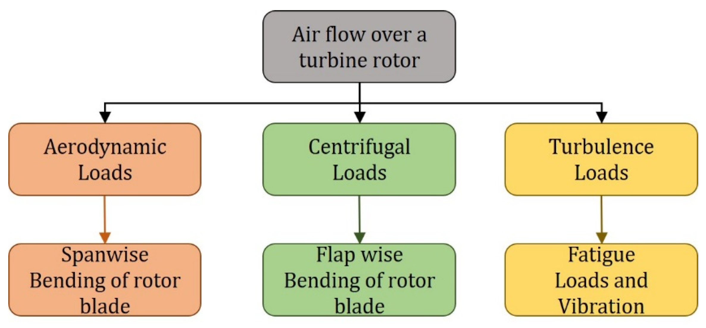
In addition to providing the rotational motion to the rotor blade, the air flow over the blade also gives rise to various loads, which may be broadly classified as aerodynamic loads, centrifugal (inertia) loads, and loads arising due to turbulence [26,27]. Figure 1 shows a schematic of how air flow would result in various loads and the consequences of these loads on the rotor blade’s structural integrity. The aerodynamic loads arise from the lift (perpendicular to wind direction) and drag (parallel and along the direction to wind) forces. The lift and drag force would change along the span of the blade; this gives rise a moment and result in the bending of the blade [27]. The bending moment would lead to stress at the root of the blade, and if the wind speed varies, then the load and the stress would also change. Centrifugal loads arise due to the rotating motion of the blade. The centrifugal load would cause moments that would rise to the pitching of the blade [26]. The pitching may push the blade out of the rotating plane and would lead to more abnormal bending of the blade. The turbulence of the wind and associated phenomena like wake are common in wind turbine aerodynamics. The turbulence causes a fluctuation of pressure difference across the blade’s faces, leading to dynamic loading, causing effects like vibration and fatigue [26]. Therefore, the most crucial factor that influences a wind turbine system’s lifetime and reliability is the loads generated by the flow of air over the blade, which is dependent predominantly on wind conditions [27].

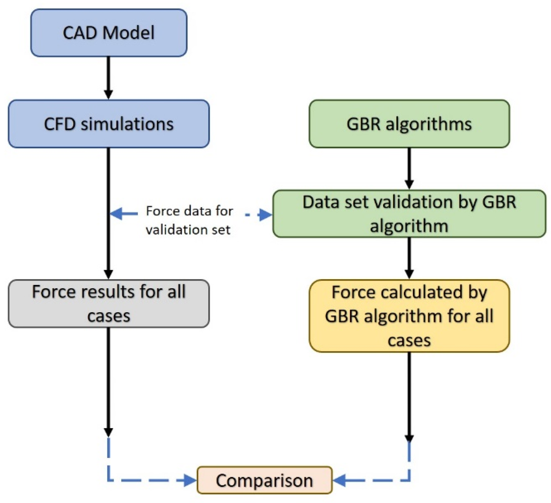
Figure 2 shows the step-by-step methodology adopted in the present study to combine machine learning and CFD. Section 3 gives the details of the CFD, and the details of the machine learning will be in Section 4.

3. Computational Fluid Dynamics (CFD) Methods

The current section describes various aspects of CFD simulation, like the model, mesh, input parameters, simulation methodology, and verification. The CFD simulation is carried out using ANSYS CFX 2020 R2 version.

3.1. Wind Turbine Rotor Model

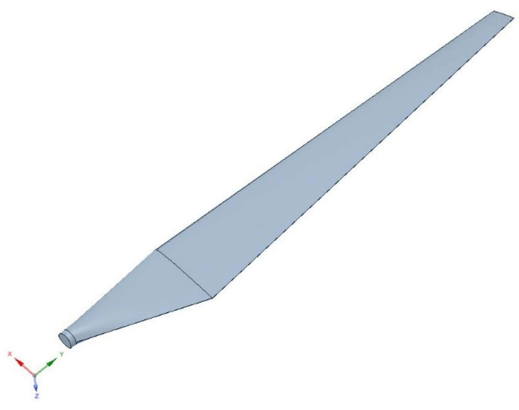
A horizontal rotational axis wind turbine is used for the analysis. The blade used in the current study comprises of NACA series (9417) obtained from the open-source online library. The blade is twisted with a top twist of 11o from root to tip. The blade radius of the rotor is 61 m. Figure 3 shows the model of the blade used in the study. As the objective here is to carry out a CFD study and focus on ML, the internal structure like spar, along with material properties, has been neglected, and only the outer profile is used for the study.

3.2. Computational Domain and Meshing

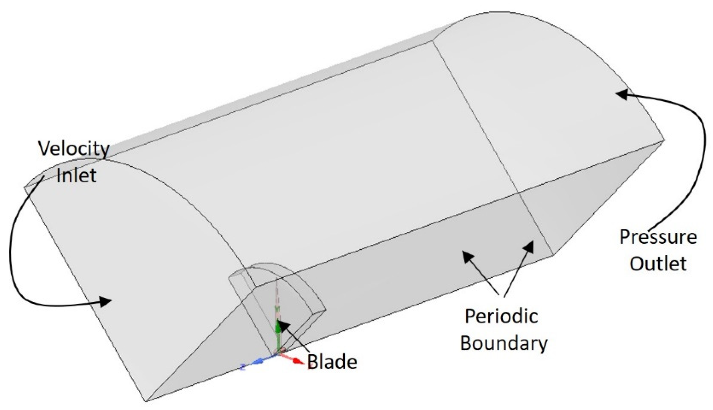
The wind turbine model is symmetrical about its centre of rotation; therefore, the three blades can be reduced to a single blade at 120° radial stream with periodic sides to reduce the solution time. Figure 4 shows the computational domain along with the boundary conditions; further details of the boundary conditions and setup are provided in Section 3.2. The blade’s location is 6.0 diameters from the inlet and 15.0 diameters from the outlet, whereas the top wall is 6.0 diameters from the tip of the blade. The computational model has the blockage ratio (ratio of the frontal area of the blade and the total inlet area) is approximately 0.004 (0.4%), which is sufficiently low not to have any artificial acceleration.

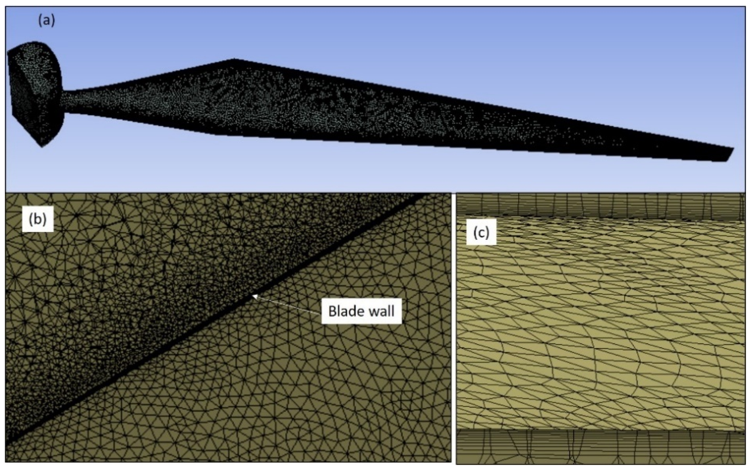
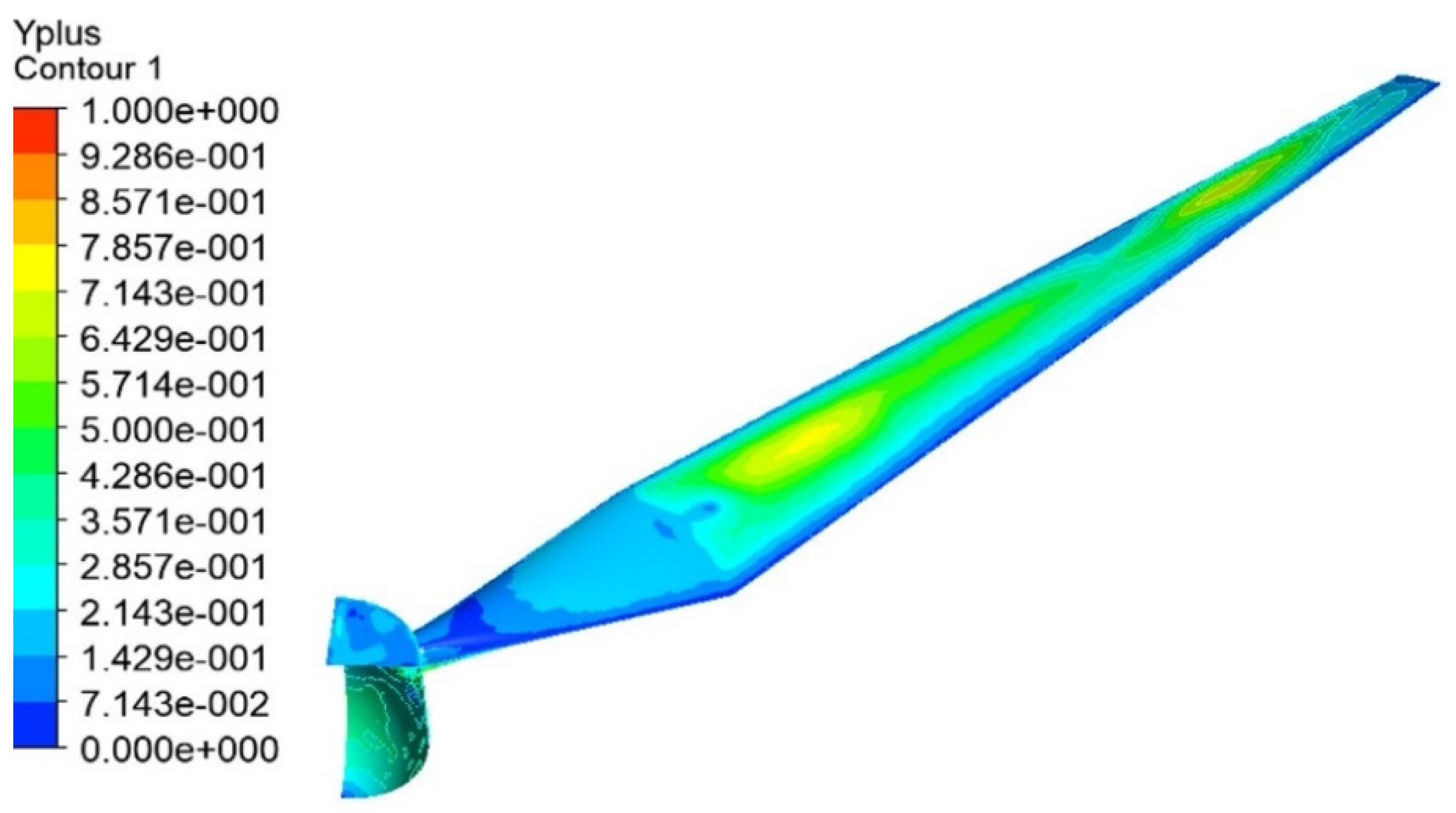
Figure 5 shows the mesh distribution at critical locations used for CFD modelling. An unstructured mesh is used with 15 layers of inflation. The first layer’s size is selected so that the y⁺ value is less than 1 for the whole blade surface, as represented in Figure 6. To determine the appropriate size of the mesh, a mesh sensitivity analysis was carried out; the details of the mesh sensitivity analysis are provided in Section 3.3.

3.3. Simulation Methodology

The CFD simulation for the present work was carried out using the ANSYS 2020 R2 CFX package. A steady-state simulation with a constant rotational speed of the rotor. The frozen rotor option of CFX was used, which is a steady-state method and uses the rotating reference frame to save the computational resources by converting transient turbo-machinery flow into a steady state. The frozen rotor option will pass the true flow to downstream and the other way around so that the wake effect downstream of the blade is captured. A shear-stress transport (SST) turbulence model was used to solve the turbulence. SST is a robust two-equation model, which has the benefit of switching from a k-ε turbulence model (well suited for far field) to a k-ω turbulence model (suited for boundary layer) [6]. As the flow over wind turbines is not high speed, it would be easy to justify the use of an incompressible flow simulation. However, even though the flow is at a low speed, but it is high turbulence, where abrupt pressure changes occur in a short distance. Therefore, in the present study, a compressible flow option is used. The basic boundary conditions are shown in Figure 4. The rotor is given a constant rotational speed of 15 rpm (frozen rotor), with inlet velocity that varied from 0–20 m/s. The pressure is held at atmospheric at the outlet. All the walls are modelled as no-slip. A 1 × 10⁻⁴ convergence criterion was used for the simulation. Once the solution was converged, and results obtained, the results such as forces, pressure, velocity, and turbulence energy were plotted and will be presented in the results section of this article.

A mesh sensitivity analysis was also carried out to select an optimum mesh. For all the mesh type, the growth rate (1.1) and max size (5 m) was fixed, and only the minimum face size was varied from 0.001m to 0.5 m. For each of the mesh types, simulations were carried out at a steady state at 5 m/s wind speed, with a static rotor to get the axial Force on the blade (mid-span),

Table 1. Data from mesh sensitivity analysis.

Minimum Mesh Size (m)	Total Elements (Million)	Axial Force (N)
0.5	1.5	36,978
0.1	2.7	53,614
0.01	4.8	75,063
0.005	6.9	80,896
0.001	10	81,105

shows the results. It can be seen that after the minimum mesh size of 0.01 m the change in axial force starts to reduce. There is approximately 7.5% difference between 0.01 and 0.005 m size, and 0.25% between 0.005 m and 0.001 m. Since there is a negligible change between 0.005 m and 0.001 m, for the advantage of computational time, 0.005 m is chosen for the rest of the simulations in the present study.

For the current study, the wind speed was varied from 5–20 m/s for two angles of attack of blade 4 and 8 degrees, at a constant rpm of 15.

3.4. Gradient Boosting Regressor

Boosting is a powerful technique for combining multiple base classifiers to produce a form of the committee whose performance can be significantly better than that of any base classifier [28]. The main idea of boosting is to add new models to the ensemble sequentially. At each particular iteration, a new, weak, base-learner model is trained with respect to the error of the whole ensemble learnt so far [28]. Gradient boosting builds the model in a stage-wise fashion, as other boosting methods do, and generalizes them by allowing optimization of an arbitrarily differentiable loss function [29]. It uses the gradient descent method to solve the minimization problem and produces a prediction model in the form of an ensemble of weak prediction models, typically decision trees. As described in the earlier section of the paper, the authors have employed the gradient boosting regressor (GBR) to predict the axial force acting on the turbine blade. GBR is a generalization of gradient boosting and involves three elements, namely, a loss function (which needs to be optimized), a weak learner (used for making predictions) and an additive model (to add weak learners to minimize the loss function) [30]. The principal idea behind this algorithm is to construct the new base-learners to be maximally correlated with the negative gradient of the loss function, associated with the whole ensemble [30]. The loss functions applied can be arbitrary but, to give better intuition, if the error function is the classic squared-error loss, the learning procedure would result in consecutive error-fitting. In general, the choice of the loss function is up to the researcher, with both a rich variety of loss functions derived so far and the possibility of implementing one’s own task-specific loss. The detailed mathematical formulation of GBR is as follows. Consider an additive model of the form [29]:

$$F\left(x\right)={\sum }_{m=1}^M{\gamma }_m{h}_m\left(x\right)$$

(1)

where $h_m\left(x\right)$ are the basis functions, which are usually called weak learners in the context of boosting. GBR uses decision trees of fixed size as weak learners. Decision trees have a number of abilities that make them valuable for boosting, namely the ability to handle data of mixed type and the ability to model complex functions. As with other boosting algorithms, GBR builds the additive model in a forward stage-wise fashion [29]:

$$F_m\left(x\right)= F_{m-1}\left(x\right)+ {\gamma }_m{h}_m\left(x\right)$$

(2)

At each stage, the decision tree $h_m\left(x\right)$ is chosen to minimize the loss function L, given the current model $F_{m-1}$ and its fit $F_{m-1}\left(x_i\right)$.

$$F_m\left(x\right) = F_{m-1}\left(x\right)+arg \underset{h}{\min }{\sum }_{i=1}^{n}L\left(y_i, F_{m-1}\left(x_i\right)-h\left(x\right)\right)$$

(3)

The initial model $F_0$ is problem-specific, for least-squares regression, one usually chooses the mean of the target values. Given any differentiable loss function L, the analyst starts with an initial model, say $F\left(x\right)= \frac{{\sum }_{i=1}^n{y}_i}{n}$. He/she then iterates (until convergence is achieved) and calculates negative gradients $-g\left(x_i\right)= -\frac{\partial L\left(y_i, F\left(x_i\right)\right)}{\partial F\left(x_i\right)}$, using a gradient descent method. Finally, the analyst fits a regression tree h to the negative gradients $-g\left(x_i\right)$.

GBR attempts to solve this minimization problem numerically via gradient descent. The gradient descent direction is the negative gradient of the loss function evaluated at the current model $F_{m-1}$, which can be calculated for any differentiable loss function:

$$F_m\left(x\right)= F_{m-1}\left(x\right)+{\gamma }_m{\sum }_{i=1}^n{\nabla }_{F}L\left(y_i, F_{m-1}\left(x_i\right)\right)$$

(4)

4. Results and Discussions

In this section, the results of both CFD and Machine Learning will be presented. First, the CFD results like velocity profile, pressure distribution, and force will be discussed; this will be followed by outcomes of the machine learning.

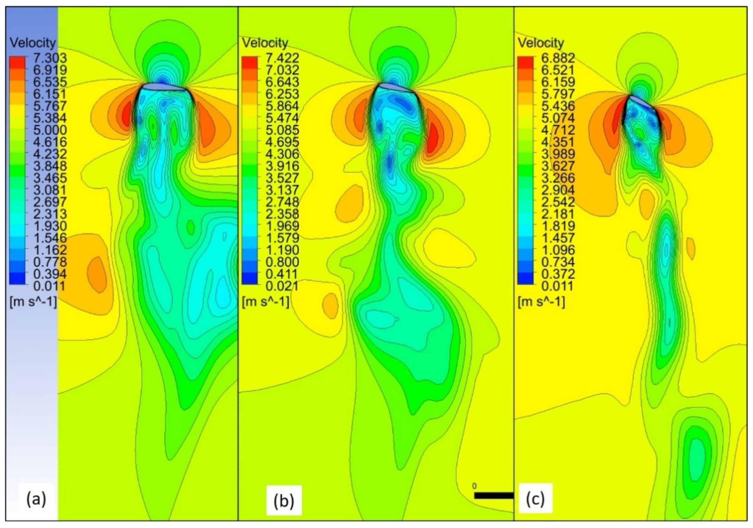
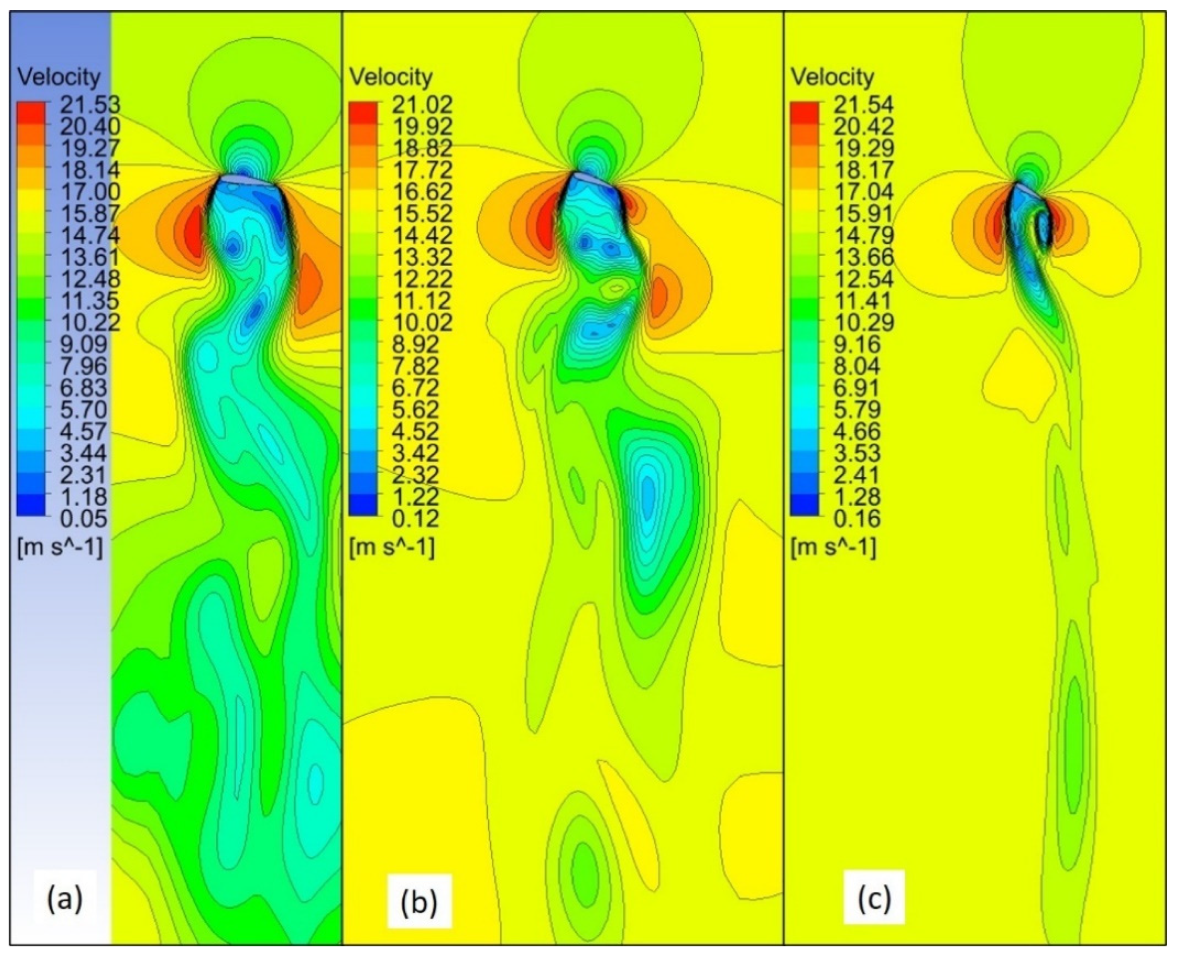
Figure 7 shows the velocity profile around the turbine blade at three sections along the span of the blade (20% (a), 50% (b) and 90% (c) of the span) at wind speeds 5 m/s and at 4° angle of attack. For both 5 m/s is a large turbulence region and formation of wake especially near the wake immediately downstream of the blade. Furthermore, it may also be noticed that the strength of turbulence increases along the length of the blade, with the maximum occurring near the tip. This is due to the twist of the blade. Therefore, there would be the difference in loading along the span of the blade, and this would influence the performance of the rotor and its power generation [31].

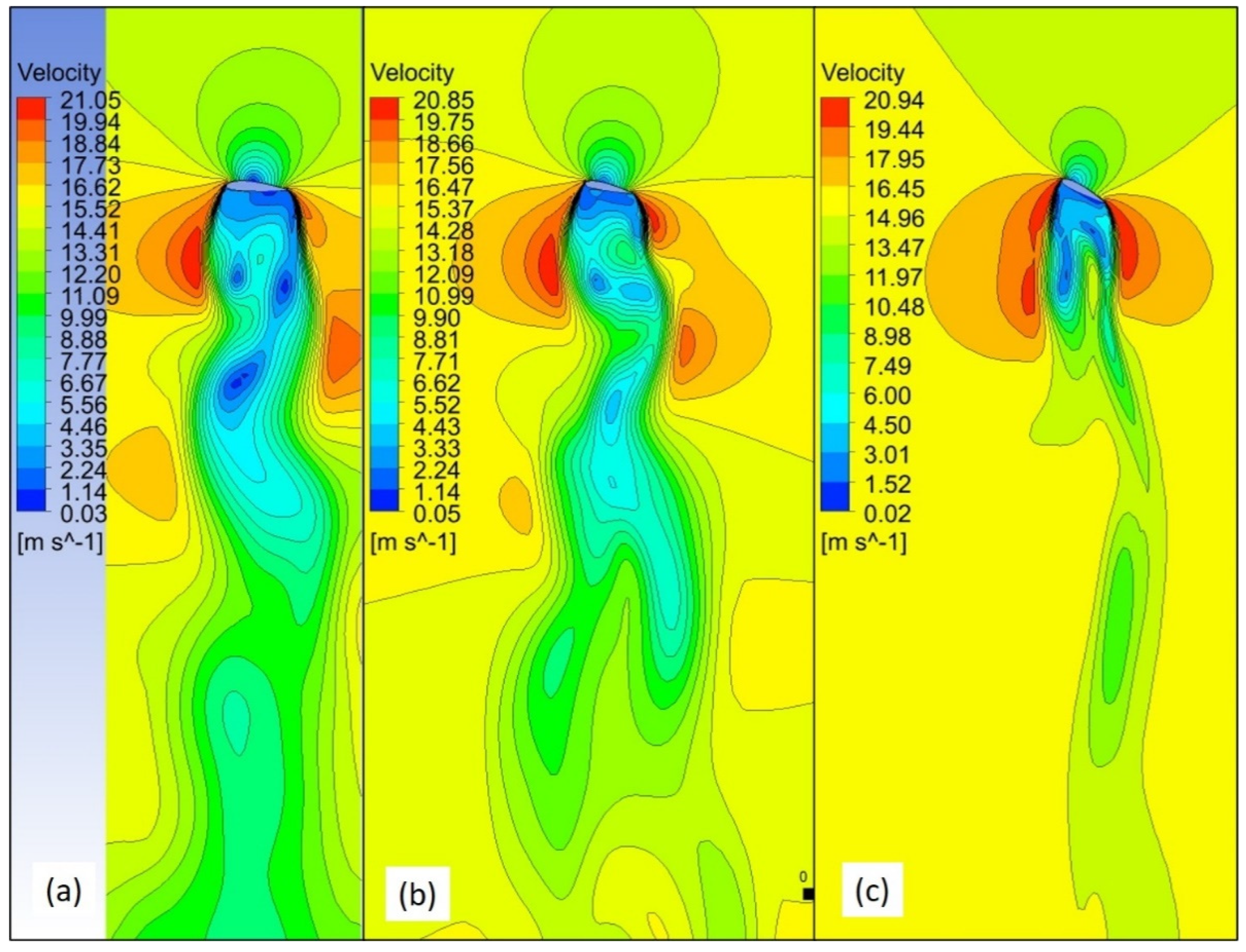
A similar observation is also seen in Figure 8 for the wind speed of 15 m/s at 4° angle of attack. However, now the turbulence is stronger, and there are more “near” wake immediately downstream of blade even at 20% section, which was not observed at 5 m/s (Figure 7a). Therefore, the stresses arising from this strong near wake and high turbulence would be higher for 15 m/s compared to 5 m/s.

Figure 9 shows the similar results at 15 m/s and 8°. Compared to 4° at 8° there are two main changes, first due to the change in the angle of attack there is a slightly larger acceleration of air around the leading and trailing edge of the blade. Secondly, there is stronger “near” wake present at the tip region (Figure 9c) at 8° compared to 4° (Figure 8c). This indicates that as inclination changes there would be more loading near the tip of the wind, which may cause severe bending stress.

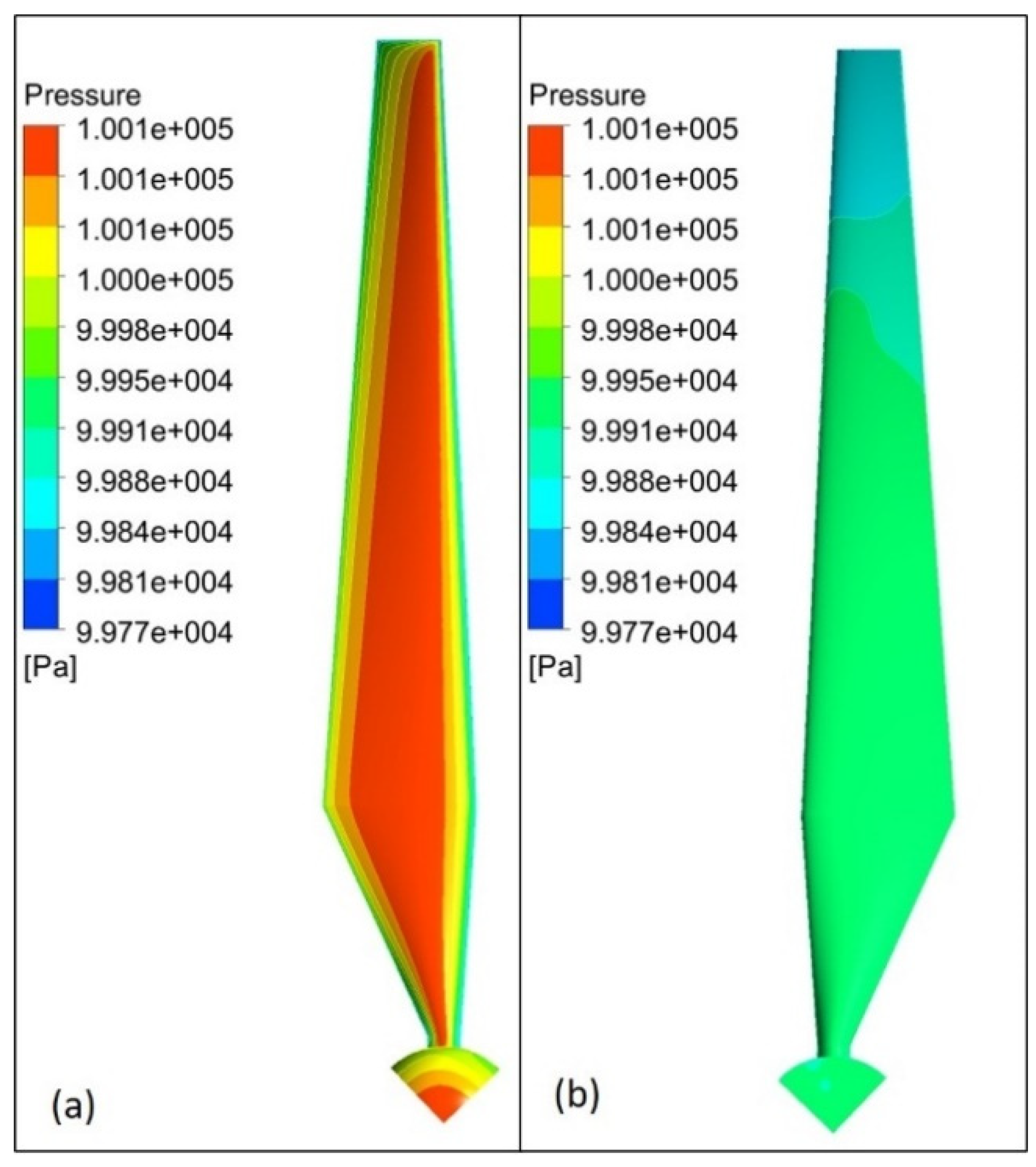
Figure 10 shows the pressure distribution over the front/leading (a) and rear (b) face of the blade a 15 m/s (4°). It is observed that on the leading face the pressure varies along the chord (width of the blade), while on the rear face the pressure varies along the span, with the lowest pressure near the tip region. The span-wise and chord-wise variation of pressure would give rise to both bending and twisting moment on the blade.

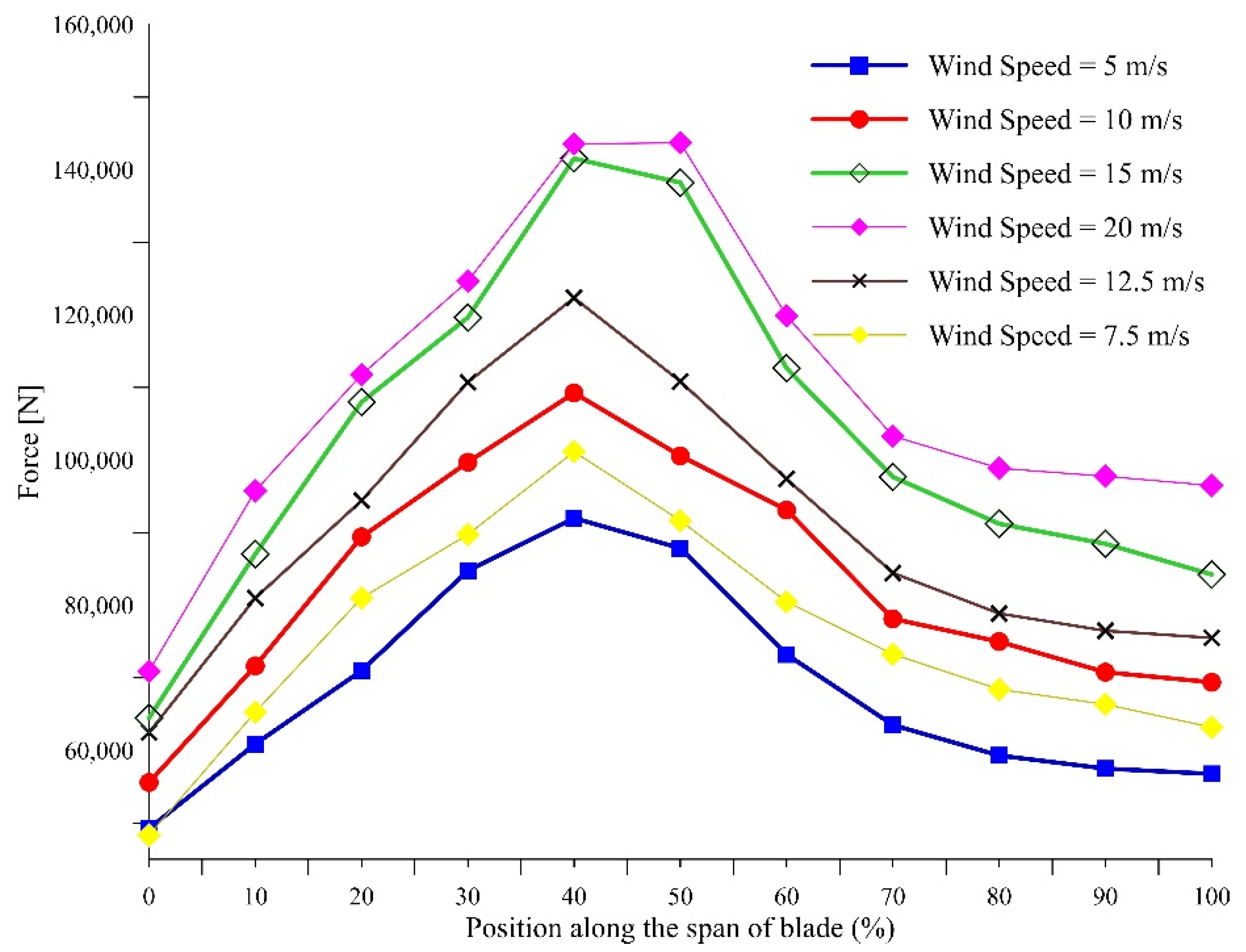
Figure 11 shows the force is axial direction at different location along the span at 4° for a wind velocity range of 5–20 m/s. The 0 in the horizontal axis represented the location of root and 1.0 represent the tip location. As expected, the force on the blade is proportional to the wind speed and for each wind speed the maximum force is near the 40% location of the span, the force reduces on the either side of this location. 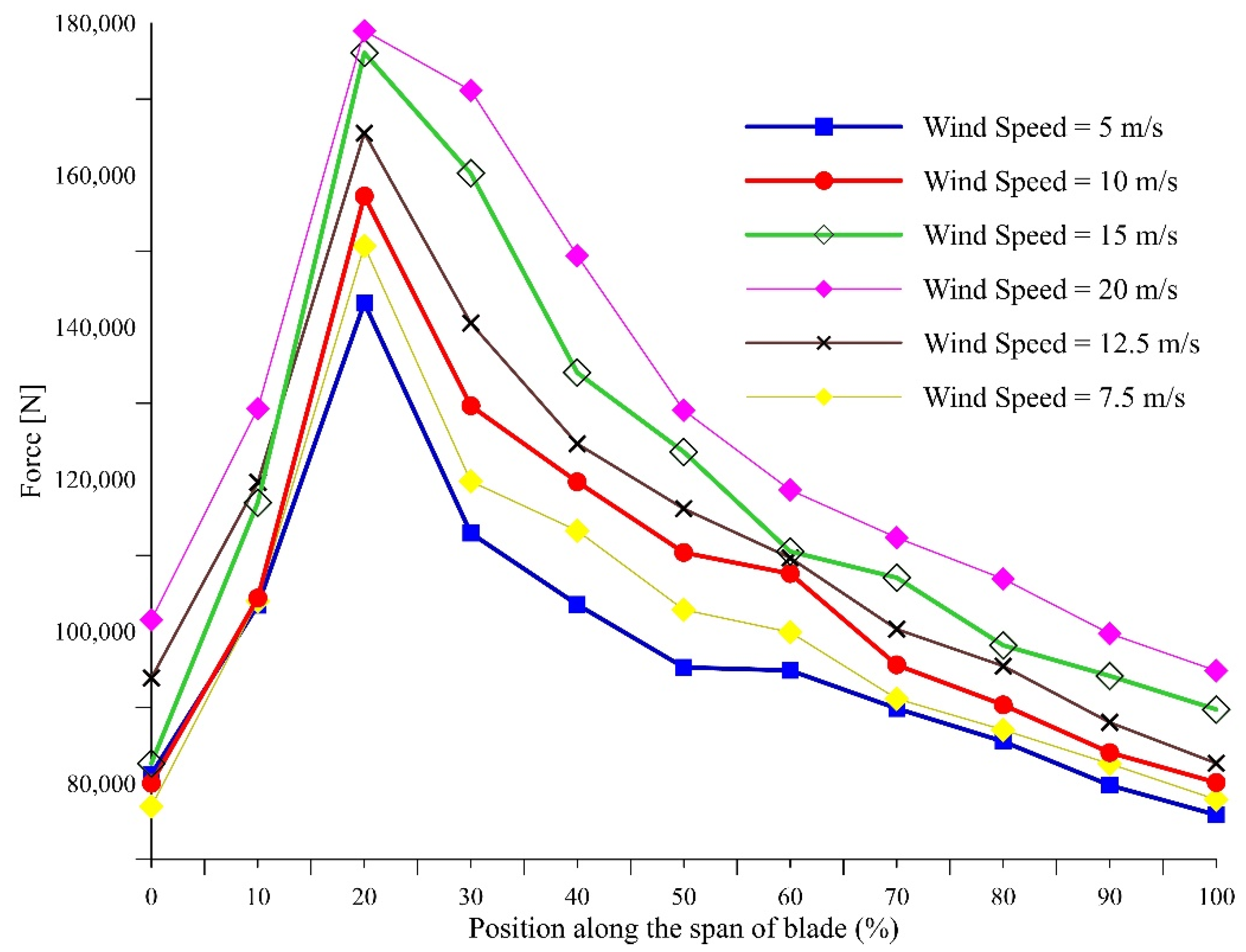Similar profile is also observed for 8° as shown in Figure 12, at same range of wind speed. The only difference is the larger magnitude and slight shift in the location of the maximum axial force location from near to 40% at 4° to near to 25% at 8°. This can be related to the formation of stronger near wake at 8° at 40% location especially at leading and trailing edges as seen from Figure 9b.

The forces presented in Figure 11 and Figure 12 shall now be used as the input dataset for the GBR algorithm.

Rather than dividing the dataset into training and testing, authors used k-fold cross validation (10 folds and 10 repeats) technique for evaluating the performance of the GBR.

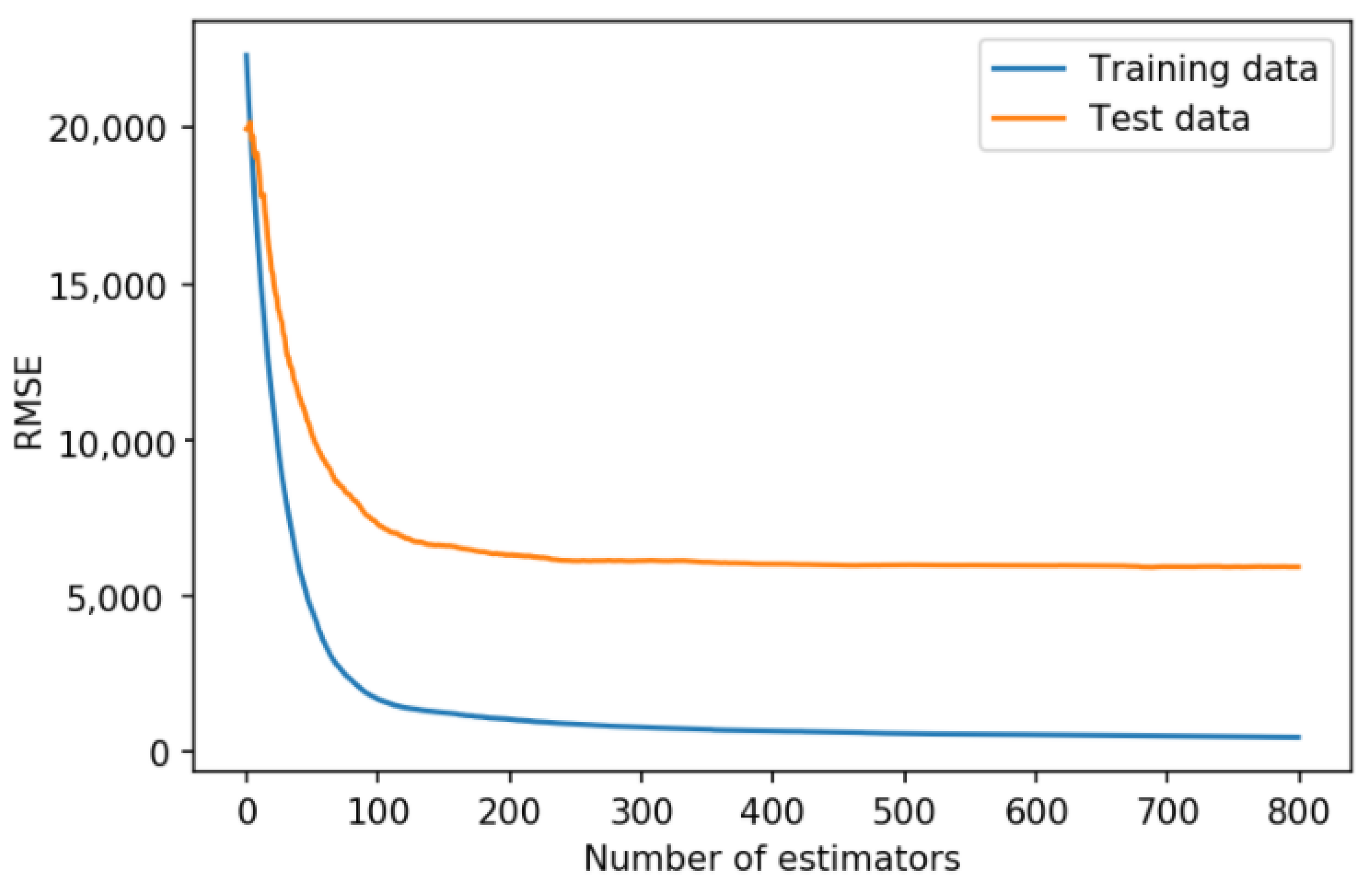
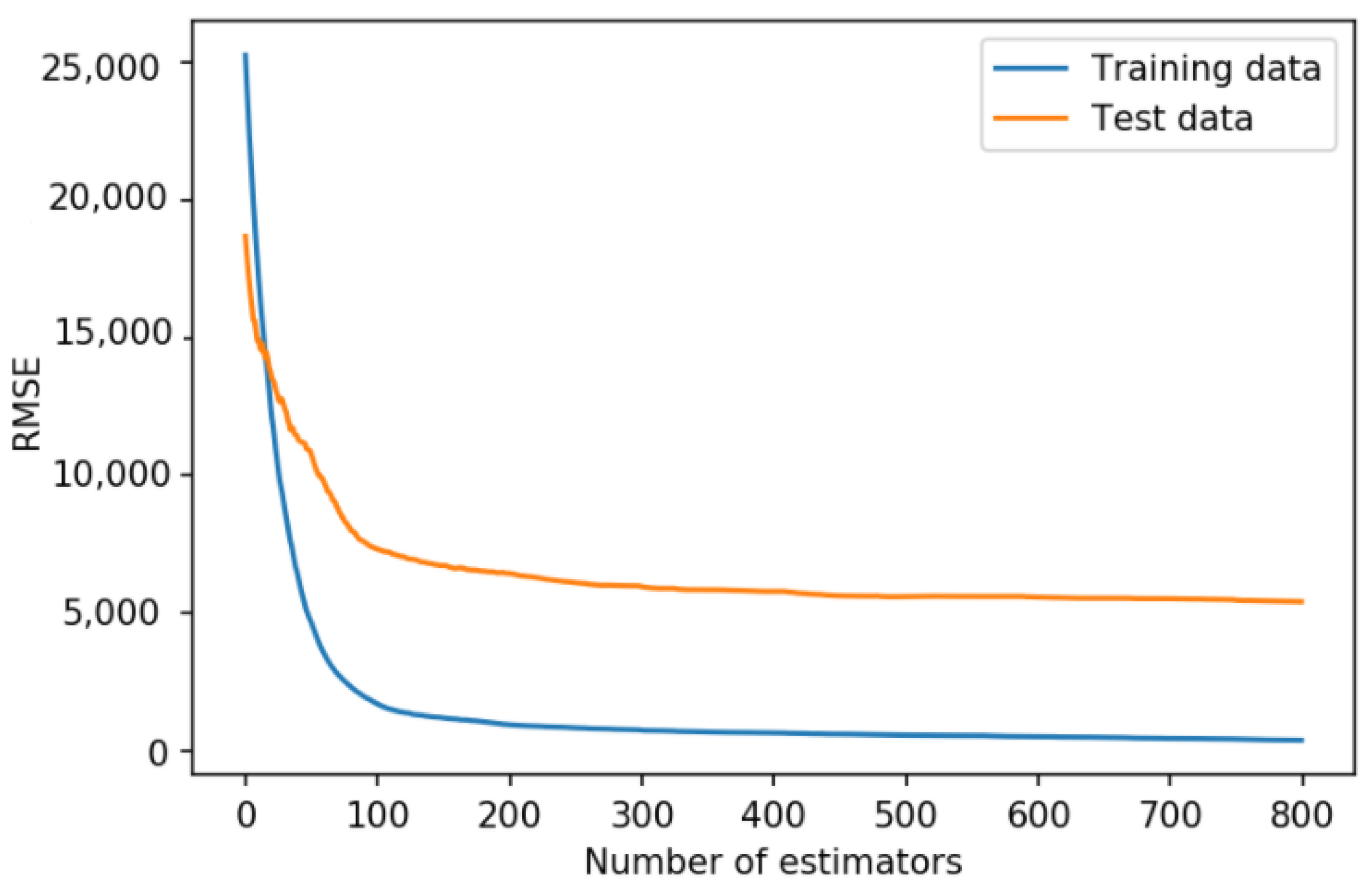
As can be seen from Figure 13 and Figure 14 for both the datasets, at around 500 estimators, the root mean square error (RMSE) for the data set becomes constant, hence 500 estimators are used for GBR. In order to compare the accuracy of the regression algorithms, three metrics, namely, RMSE, mean absolute error (MAE), explained variance score (EVS) are used. Mathematically, these are written as:

$$RMSE=\sqrt{\frac{\left({\sum }_{i=1}^n{\left(y_i-{\widehat{y}}_i\right)}^2 \right)}{n}}$$

$$MAE= \frac{{\sum }_{i=1}^n\left|y_i-{\widehat{y}}_i\right|}{n}$$

(5)

$$EVS=1-\frac{Var\left(y_i-{\widehat{y}}_i\right)}{Var\left(y_i\right)}$$

For optimal performance of the GBR, the value of RMSE and MAE should be as small as possible and the value of EVS should be closer to 1. The value of the three metrics for GBR for the analysis is shown in

Table 2. Gradient boosting regressor (GBR) prediction accuracy metrics for 4 degree and 8 degree.

Angle of Attack	RMSE	MAE	EVS
4 Degree	5281	4845	0.933
8 Degree	5386	4077	0.917

.

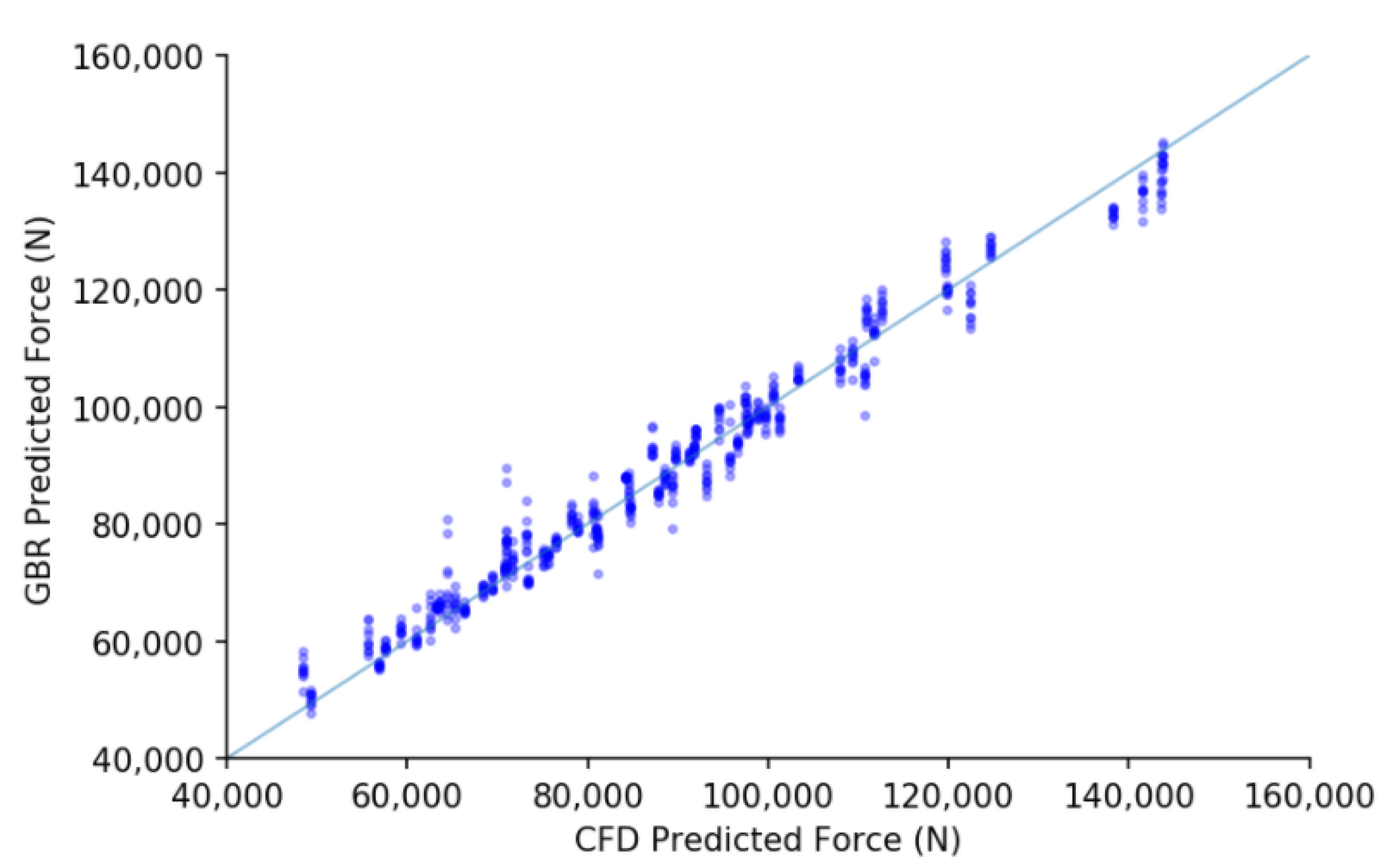
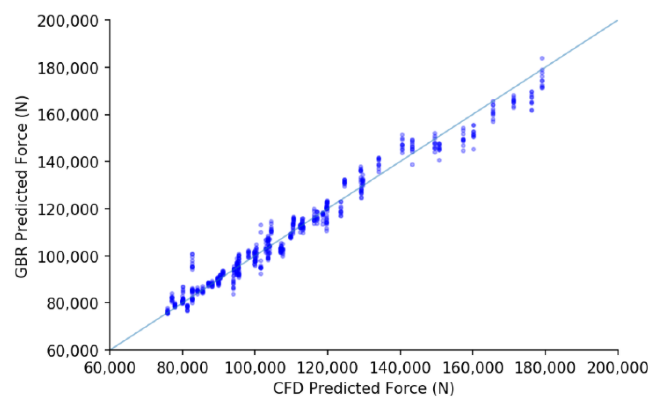
Finally, the GBR model is trained and tested on the dataset, and the plots of force predicted by CFD and GBR for two angles of attack is shown in Figure 13 and Figure 14. As can be seen from Figure 15 and Figure 16, there are very few outliers and in general the trend between the force predicted by CFD and GBR is almost linear, thus indicating good prediction accuracy of the GBR. The authors wish to express that they compared 12 different machine learning algorithms, details of which can be found in [32]. Since GBR was the most accurate algorithm, it was used to estimate the force acting on the wind rotor blade.

5. Summary and Conclusions

The study focuses on demonstrating the ability of machine learning algorithm (gradient boosting regressor in this case) to predict the wind turbine response to a combination of wind speed, angle of attack, and turbulence intensity when the air flows over the rotor blade. The focus and novelty of the present study is in the machine learning part. CFD simulations were carried out to estimate the axial force for the wind speed range of 5–20 m/s, for two different orientations of the blade with regard to wind direction.

GBR was successful in satisfactorily replicating the Force estimated by CFD. High prediction accuracy and less time consumption makes GBR a suitable alternative for CFD to predict force at different wind velocities for which CFD analysis has not been performed. In future work, the authors wish to extend the current work by:

• Improving the prediction accuracy of GBR by employing hyperparameter tuning.
• Utilizing the force predicted by GBR to estimate vibration-induced stresses in the blade, which in turn can be utilized for estimating fatigue life of the blades by performing probabilistic crack growth analysis. Thus, the research presented in this manuscript forms the foundation of the future research centered around predicting vibration-induced fatigue failure of the rotor blades.