Applicability of a Three-Layer Model for the Dynamic Analysis of Ballasted Railway Tracks

Abstract

In this paper, the three-layer model of ballasted railway track with discrete supports is analyzed to access its applicability. The model is referred as the discrete support model and abbreviated by DSM. For calibration, a 3D finite element (FE) model is created and validated by experiments. Formulas available in the literature are analyzed and new formulas for identifying parameters of the DSM are derived and validated over the range of typical track properties. These formulas are determined by fitting the results of the DSM to the 3D FE model using metaheuristic optimization. In addition, the range of applicability of the DSM is established. The new formulas are presented as a simple computational engineering tool, allowing one to calculate all the data needed for the DSM by adopting the geometrical and basic mechanical properties of the track. It is demonstrated that the currently available formulas have to be adapted to include inertial effects of the dynamically activated part of the foundation and that the contribution of the shear stiffness, being determined by ballast and foundation properties, is essential. Based on this conclusion, all similar models that neglect the shear resistance of the model and inertial properties of the foundation are unable to reproduce the deflection shape of the rail in a general way.

1. Introduction

Numerical models of the railway track are fundamental tools for the study of their dynamic behavior, with implications for the safety and comfort of rail transport. The importance of these models has increased alongside the speed of the railway vehicles and capacity of the network over the last decades.

The use of 3D FE models is common practice, but reduced models are still relevant, due to simplicity of implementation and results interpretation, and low computational cost. Despite the wide use of the reduced models, there are still relatively few studies about their overall applicability and how to select appropriate parameters based on the properties of the railway track. Most works determine the necessary parameters in a way to match the response of the model to experimental measurements from the track. This means that the range of applicability of the methods developed and the conclusions reached in these works are always, to some extent, limited.

This paper provides a detailed analysis of the viability and applicability of the three-layer discrete support model [1], for simplicity referred to as the discrete support model and abbreviated by DSM, expanding on the work presented in [2] and analyzing the formulas proposed in [3]. The DSM is a 2D model composed of a beam, representing the rails, connected to sets of springs, dampers and masses that represent the support elements of the track: the fastening system, sleepers, ballast, and subgrade. The DSM has significant advantages over the more detailed 3D FE model, which presents a high computational cost, large number of results to analyze, the need for special boundary conditions, necessity for high level of discretization, etc. Given its computational efficiency, the DSM and other, even simpler models, are often used to study complex phenomena that arise in different railway transportation problems. Examples of published works dealing with specific railway problems include: (i) modelling the vehicle–track dynamic interaction on plain line [4,5,6,7,8,9,10,11,12,13] but also in the case when the line is passing over bridge [14] or crossing a transition zone [15,16]; (ii) assessing and diagnosing the deterioration of track components [17,18,19,20,21,22], including switches and crossings [23,24,25], rail wear/corrugation [26,27,28,29] and hanging sleepers [30,31]; (iii) studying other problems related to wheel–rail interaction, including the effect of wheel flats [32,33,34,35,36,37] and rolling noise [38,39,40,41,42].

Published works with the aim of defining the properties of reduced models with discrete supports consider the ballast pyramid model referred to in [43,44] and the Saller assumption from 1932 which can be consulted in [45]. The pyramid model is further detailed in [4], under the name stress cone model, where it is used not only for the definition of the vertical ballast stiffness, but also for the identification of the oscillating ballast mass. Further improvements include the superposition of the cones between adjacent sleepers, i.e., in the longitudinal direction [3]. Nevertheless, these works have two notable limitations: (i) they do not propose theoretical expressions for all the elements of the model, (ii) they each validate their models and theoretical expressions by comparison with experimental measurements of a single railway track, and therefore cannot prove that they are widely applicable to a range of different track properties. The two limitations are particularly serious when considered together; since some parameters of the models are obtained by fitting its results to experimental measurements for a single set of track parameters, it is not possible to unequivocally determine if the other parameters are intrinsic to the physical phenomena, or if the good approximation is obtained simply by virtue of the fitting process.

Therefore, the present work aims to provide a detailed analysis of the viability and applicability of the DSM, to derive formulas for its components that are still missing and to enhance formulas that are already available. This is achieved by fitting the DSM steady-state vertical displacement of the rail under moving force to reference solutions that cover a wide range of representative values of the track. The reference solutions are obtained by a linear elastic 3D FE model, which is validated by the experimental measurements published by Paixão [46]. The use of a linear elastic model is appropriate because the focus is on the track’s short-term dynamic behavior. Analyzing the deflection shape of the rail is also adequate, because obtaining a good approximation of the steady-state rail displacement is a necessary prerequisite for studying more complex phenomena.

The DSM is fitted to the reference solutions using genetic algorithms, first individually for each combination of track parameters, to evaluate its ability to approximate the results of the 3D FE model and to define proportionality relationships between the properties of the track and those of the DSM. After that, optimization is conducted simultaneously for various combinations of track parameters. Based on these results, theoretical expressions for all parameters of the DSM are derived as functions of the geometry and mechanical properties of the track. It is shown that the currently available formulas have to be adapted in a way to include inertial effects of the dynamically activated part of the foundation and that the contribution of the shear stiffness which must account not only for ballast but also for foundation, is essential. This is in agreement with [47,48], where it is shown that if the shear stiffness of the model is neglected, then the critical velocity of a uniformly moving force tends to zero with the dynamically activated mass of the model, which is not physical. With this conclusion, all similar models that neglect the shear resistance of the model and inertial properties of the foundation are unable to reproduce the deflection shape of the rail in a general way. In addition to these new conclusions, the stress cone formulas are improved by incorporating the superposition of the cones in the lateral direction. All formulas are presented as a simple computational engineering tool, allowing the reader to calculate all the data needed for the DSM simply by adopting the geometrical and basic mechanical properties of the track constituents.

This paper is organized in the following way: Section 2 describes the DSM and reviews the relevant literature, Section 3 presents the 3D FE model and its validation, Section 4 is dedicated to the calibration of the DSM based on the results of the 3D FE model and derivation of the theoretical expressions and Section 5 summarizes the main conclusions.

2. DSM

Regarding the evolution of the reduced models, it is worthwhile to mention that discrete supports were introduced in [49] to remove the limitations of the Winkler and Pasternak models, which consist of a beam continuously supported by an elastic or viscoelastic foundation. Newton and Clark [50] were the first to use the abbreviation DSM and to consider the sleepers as discrete mass elements, which separated the stiffness and damping introduced by the fastening system from the one due to the ballast bed and subgrade, creating two layers. In [51], another set of masses that represent the ballast were introduced, and therefore, the stiffness and damping of the ballast and of the subgrade/foundation got also separated, creating three layers. 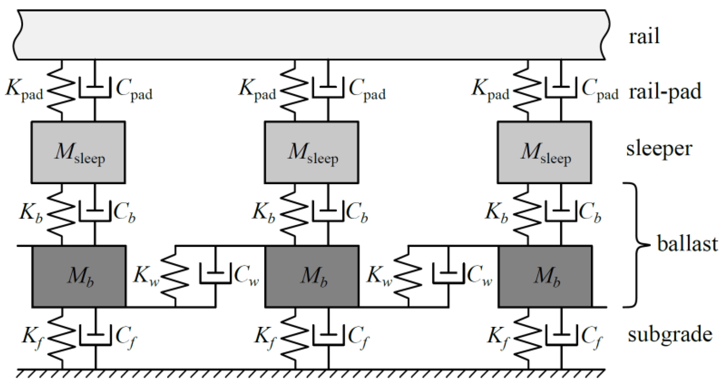Zhai and Sun [4] then introduced springs and dampers connecting consecutive ballast masses to model the shear behavior of the ballast, which already cover all the DSM components, as depicted in Figure 1.

The rail is modelled as a Timoshenko beam, for which the bending ($EI$) and shear stiffness ($GA*$), and the mass per unit length ($m$) are well-known. Likewise, the fastening system stiffness and damping coefficient ($K_{pad}$ and $C_{pad}$) can be determined experimentally. The sleepers experience very little deformation during the normal use of the track, so they are modelled as rigid elements that only contribute with their mass ($M_{sleep}$), which is well-defined. The remaining unknown parameters are the vertical stiffness and damping coefficient of the ballast ($K_b$ and $C_b$), the vertical stiffness and damping coefficient of the subgrade ($K_f$ and $C_f$), the shear stiffness and damping coefficient of the ballast ($K_w$ and $C_w$) and the dynamically activated ballast mass ($M_b$).

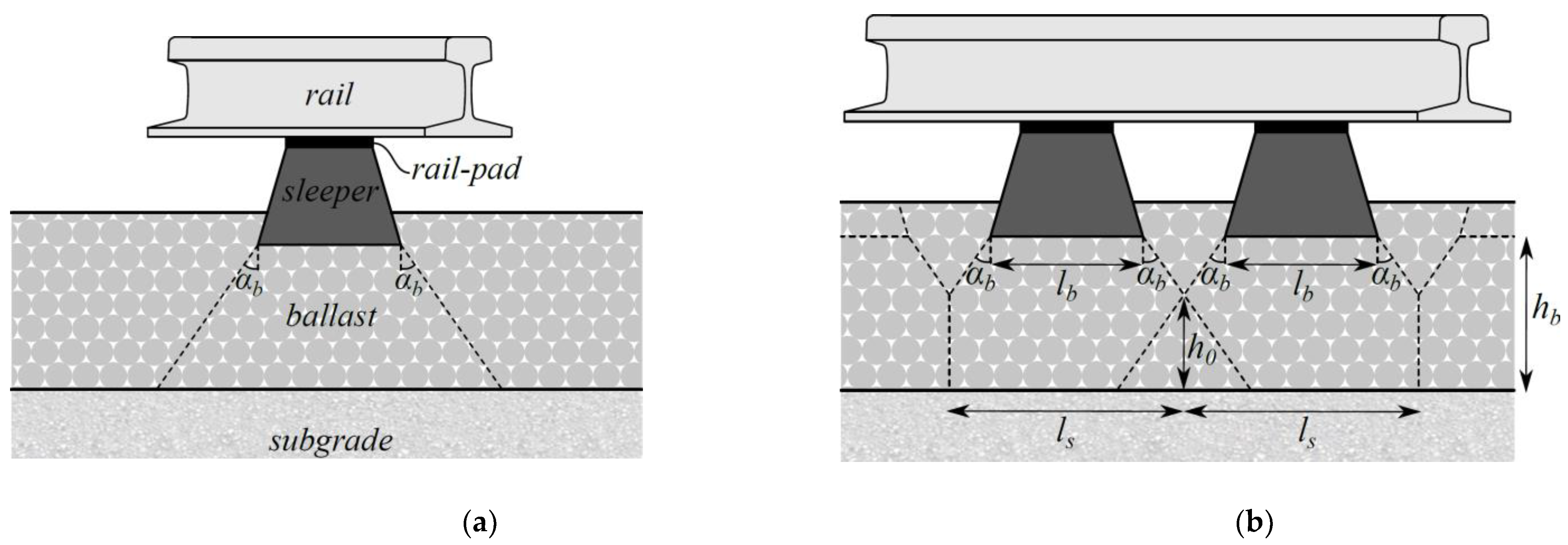
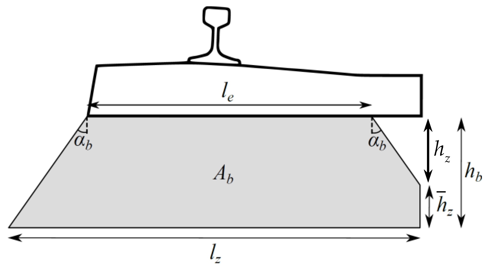
In [3,4], formulas for calculation of the vertical stiffness of the ballast are proposed as an adaptation of the stress cone (pyramid) method, which assumes that the stresses are transmitted from the effective load-bearing area under the sleepers to the ballast, and then dissipate at a constant angle, as shown in Figure 2a. The effective load-bearing area under the sleepers is determined in [45], based on experimental observations and simple geometrical considerations, requiring only the sleeper’s dimensions and the track gauge. Then, the vertical stiffness $K_b$ can be determined as a function of a distribution angle ${\alpha }_b$, the Young modulus of the ballast and its depth. In [43], a reduction factor for the vertical stiffness due to superposition of stress cones of 0.5 was proposed based on experimental observations. In [3], superposition of the adjacent stress cones in the longitudinal direction is introduced exactly. The cone volume such defined is then used for the estimation of the dynamically activated ballast mass, $M_b$. The area of the base of the stress cone is further used to calculate the foundation vertical stiffness, $K_f$, but for this, the experimentally determined subgrade reaction modulus must be known.

No functional dependence is proposed for all damping coefficients ($C_b$, $C_f$ and $C_w$), for the shear stiffness of the ballast ($K_w$) and, in fact, also for the foundation stiffness $K_f$. There is also no justification for the value of the distribution angle ${\alpha }_b$. It is therefore the objective of the present work to propose general formulas for all components of the DSM without the necessity to call on experimental data. Alongside this, the range of applicability of the DSM is obtained. Contrary to the arrangement given in Figure 1, it is proven that the dynamically activated part of the foundation must be added to the ballast mass and that the shear stiffness of the ballast must be increased by the contribution from the foundation soils. If this is not respected, then the DSM is unable to reproduce the deflection shape of the rail in a general way.

3. Three-Dimensional Model

To obtain the reference results necessary to calibrate the DSM, a 3D FE model of the railway track is developed. This model has linear elastic behavior and can be used to obtain static and dynamic vertical displacements in the rail. It is implemented using the ANSYS parametric design language [51], so the model can be generated in a fully automatic way for each set of parameters.

Static, modal and transient analyses are used to define the necessary discretization and which type of boundary conditions (BCs) are suitable to the problem in study. The static and modal analyses are necessary to validate the stiffness component of the BCs. The 3D FE model is validated by modelling an existing railway track for which the rail displacements due to a train passage are available in [46].

The sleepers, ballast and subgrade are modelled by brick and wedge solid elements, and beam elements are used for the rail and discrete spring–damper elements in the three orthogonal directions simulate the fastening system. The Timoshenko beam has the cross-section properties of a 60E1 rail profile [52] and shear factor of 0.4 as in [5]. The sleepers are spaced by 0.6 m and their geometry is based on the DW post-tensioned mono-block concrete sleepers used by the Portuguese railway manager, I.P. S.A. 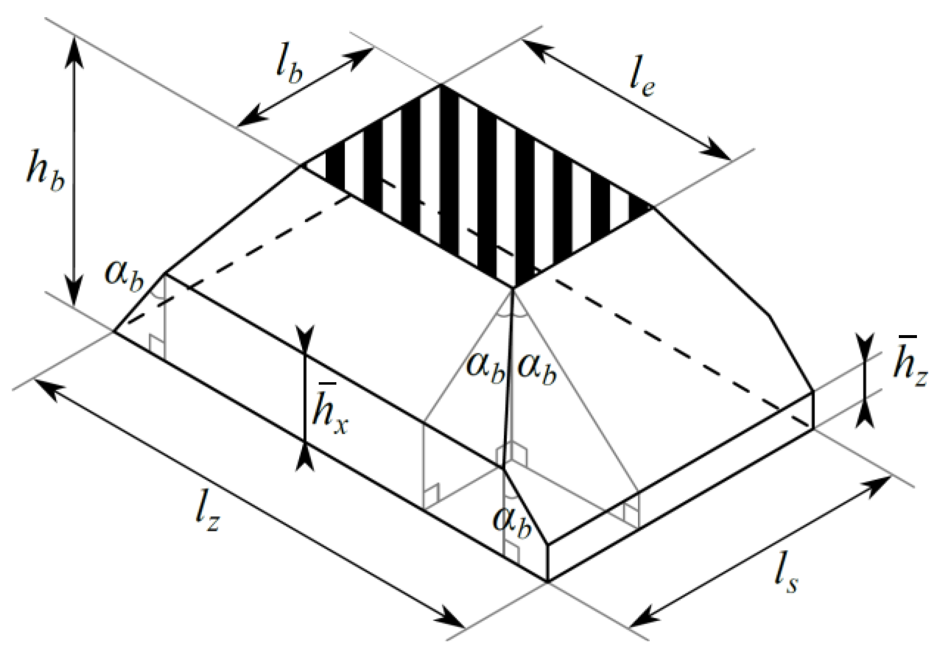[53,54], but altered to achieve a regular mesh (the following parameters in m are used: length 2.6, bottom width 0.3, top width 0.2 and height 0.22). The moment of inertia is approximately the same as the real section, and the change in volume is corrected by applying a factor to the mass of the material of 0.86. Another simplification is that no loss of contact is possible between distinct materials, however, in the absence of sudden changes in stiffness or other irregularities, no loss of contact occurs anyway. Symmetry along the vertical plane parallel to the rails (the xy-plane) is assumed, reducing the size of the model to half, as seen in Figure 3. The shoulder width of 0.5 m and slope 1:2 are assumed for the ballast layer. Two thicknesses will be used of 0.3 and 0.6 m, leading to the bottom width of 4.8 and 6 m. The subgrade is discretized using a regular orthogonal mesh. The regularity of the mesh simplifies the process of implementing BCs and avoids spurious reflections between elements of different sizes [55]. Preliminary tests have also shown that the BCs perform worse at the interface between different element sizes. Convergence studies for static, dynamic and transient analyses led to the choice of the mesh: rail (x) 0.05 m; longitudinal direction (x) 0.075 m, lateral (z) and vertical direction except for sleepers (y) 0.1 m, along sleeper height (y) 0.055 m.

The subgrade depth can be defined as the depth at which a significantly rigid substrate is found, or as a reasonable depth after which the deformations due to surface loads are negligible (the so-called active depth of the soil [56,57]). A great variety of such values can be found in the literature: some adopt values of the order of 3 m [58,59], while others consider much higher values, from 10 m [60,61] to 50 m [62,63,64] and as high as 70 m [65]. Given this variability, five different depths of the subgrade ($h_s$) are studied: 3, 6 and 9 m (relatively shallow subgrade), 25 m (an average depth) and 50 m (a high depth). Not all the depths are considered for all the different analyses, as will be discussed in the relevant section.

All materials are assumed to have linear elastic behavior, since the purpose of the model is to analyze short-term behavior due to vehicle passage. Besides the elastic components, there are discrete linear viscous dampers in the fastening system. No material damping was considered in the ballast and subgrade, to avoid damping the dynamic response. The material properties of the rail and sleepers are well defined, since they are manufactured components that follow the relevant standards [53,54]. The properties of the ballast and subgrade, on the other hand, show great variability across the literature, particularly the Young modulus (see Rodrigues [66]), which generally has the greatest influence on the short-term response of the track. Three values of the Young modulus were chosen for the ballast and subgrade, which cover the relevant range found in the literature while excluding extreme values that are not representative of typical railway tracks in good condition.

Table 1. Elastic material properties for the three-dimensional railway model.

Property	Rail	Sleeper	Ballast	Subgrade
Young’s modulus [MPa]	210∙103	38∙103	50,100,150	50,100,150
Poisson’s ratio	0.3	0.2	0.25	0.35
Density [kg/m3]	7850	2064 1	1750	1900

¹ Modified by correction factor.

summarizes these values, the most typical values of Poisson’s ratio and mass density and the properties of the sleepers and rail.

The range considered for Young’s modulus of the ballast may be considered large, but it was justified by extensive literature search and by summarizing values from more than 40 sources. The histogram for ballast Young’s modulus, Poisson’s ratio and density are presented in Figure 4.

For the properties of the fastening system, the Vossloh Zw687a EVA rail pad with direct fastening is used, to match IP S.A. [54]. In agreement with [67], the static stiffness of 1300 MN/m and 100 MN/m, dynamic stiffness of 3550 MN/m and 280 MN/m and damping coefficient of 36 kNs/m and 10 kNs/m were used, with the first value reflecting the vertical and the second value the lateral and longitudinal directions, respectively (see [66] for more details).

In regard to the elastic part of the BCs, the normal stiffness of $4G/r$ and tangential stiffness of $2G/r$ is used at the lateral surfaces, as derived for spherical waves in [68,69], because they were found to work better than the ones derived for the cylindrical waves that were used in [70]. The bottom boundary is considered either fixed or $E^{oed}/h$ and $G/h$ are used for the normal and tangential stiffness, respectively, as in [70]. Here, $G$ stands for the shear modulus, $r$ for the distance from the source, $E^{oed}$ is the oedometric modulus and $h$ is the depth of the foundation not being modelled. At all (non-fixed) boundaries damping coefficients of $\rho c_p$ for normal and $\rho c_s$ for tangential direction, as in [68,69,70,71] are used. Here, $\rho$ is the density and $c_p$, $c_s$, are the velocity of propagation of pressure and shear waves, respectively.

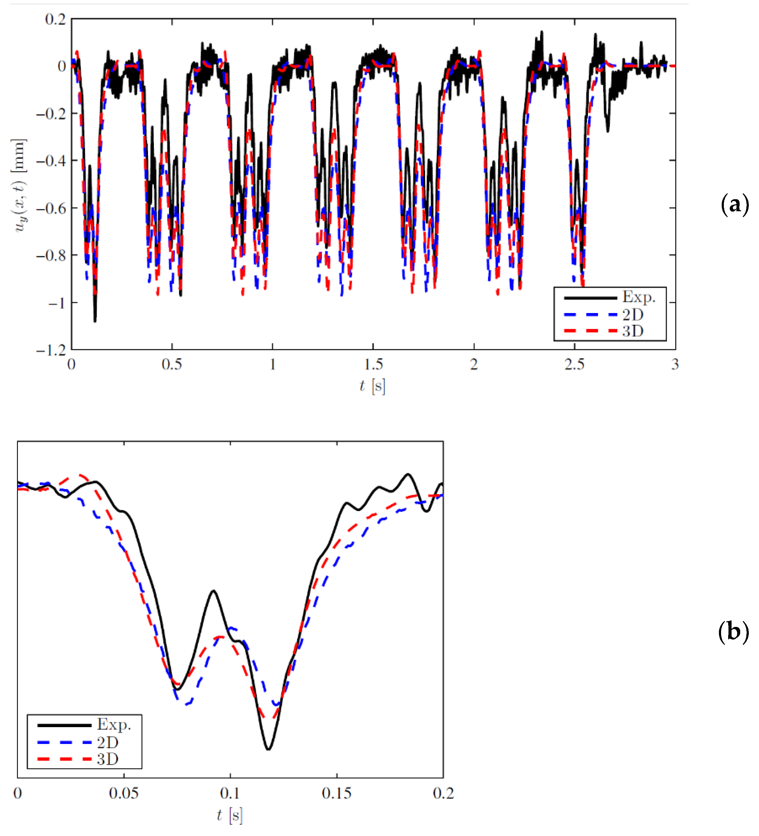
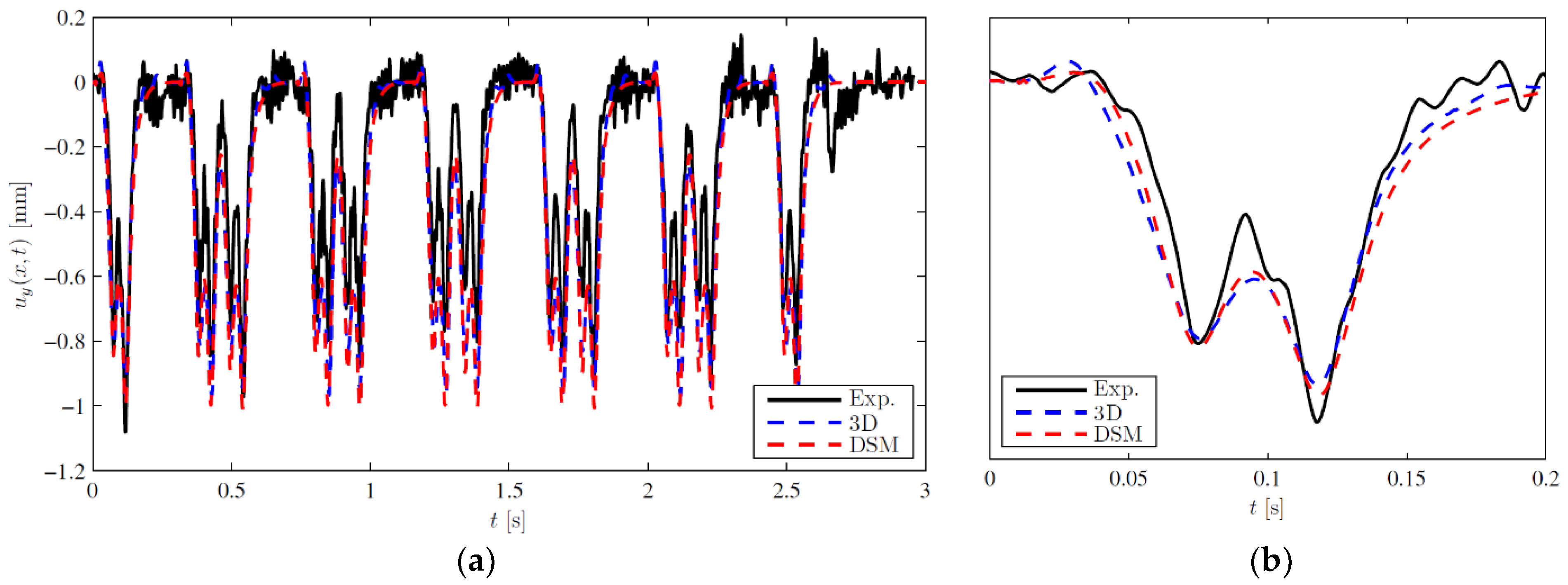
The model was tested for different combinations of properties and showed good convergence for the mesh specified for static displacement, the 10 first natural frequencies, the transient response to a pulse load and to a moving load at velocities of 50 and 100 m/s. Finally, the model was validated by comparison with results published in [46], where the measured vertical vibrations of a railway line in Portugal due to the passage of a train at 220 km/h are compared to the results of a 2D FE model. 66 kN per wheel is used in the front bogie. By adapting the properties of the 3D FE model developed for the purpose of this paper, the vertical displacements seen in Figure 5 were obtained.

It can be concluded that the 3D FE model provides a good approximation to the experimental results, particularly when taking into account the variability of the track properties and the random nature of the dynamic response for high frequencies due to the short-wave irregularities of the rails and wheels. These results also confirm that the simplifications introduced in the model do not significantly impact its applicability, namely, the assumption of linear elasticity and the use of moving forces.

The input data for the 3D FE model are taken from [46]. Besides the typical properties related to the rail, rail pads and sleepers, there are other materials characterized by its thickness, Youngs’s modulus, density and Poisson’s ratio: the ballast layer (0.3 m, 130 MPa, 1530 kg/m³, 0.2), sub-ballast layer (0.3 m, 200 MPa, 1935 kg/m³, 0.3), capping layer (0.2 m, 2820 MPa, 1935 kg/m³, 0.3), embankment soils (~7 m, 80 MPa, 2040 kg/m³, 0.3) and natural foundation (~3.5 m, 300 MPa, 2040 kg/m³, 0.3). The depth of the embankment soils and the stiffness of the natural foundation in relation to that of the former were deemed high enough that the latter can be considered as a rigid substrate, therefore subgrade was implemented with (7 m, 80 MPa, 2040 kg/m³, 0.3) because the capping layer, having low thickness, does not influence the equivalent stiffness much. As far as the ballast layer, as the generic model used for optimization has only one layer, (0.6 m, 150 MPa, 1530 kg/m³, 0.2) was implemented, where 150 MPa corresponds to an equivalent modulus obtained by considering the two layers characterized by equivalent springs connected in series.

4. Optimization

The optimization is performed using genetic algorithms (GA), which, being a heuristic method, provides no guarantee that the solution found is the global optimum. Therefore, several independent runs are necessary to guarantee the stability of the results obtained. In what follows, only stable results will be shown for each set of optimization runs, for the sake of brevity. For all optimization runs, the following parameters are used: the population consists of 100 individuals, the number of generations is 20, the mutation rate is 1% and an elite of two individuals is kept between generations (see [72] for definitions). The objective function $\mathsf{\Phi }$ is equal to the L²-norm of the difference between the rail displacements resulting from the DSM and from the 3D FE model, divided by the L²-norm of the displacement obtained by the 3D FE model. Therefore, $\mathsf{\Phi }$ can theoretically reach zero when both deflection shapes are identical.

The philosophy behind the optimization is the following: firstly, dependence on basic mechanical properties is determined, identifying the proportionality factors; secondly, mechanistic expressions are used to specify these proportionality factors in terms of some geometric or similar specifications of the model. This is very important because the solution of the optimization problem is not unique, i.e., several combinations of parameters can lead to practically identical rail deflection shapes, but for some of those solutions, the parameters have no physical meaning. Expressing the proportionality factors in terms of some geometric parameters impose natural limits on the design space and consequently guarantee the obtainment of physically admissible values.

Besides this, the optimization is divided in two steps. First, the stiffness parameters characterizing the DSM are determined from the static analysis ($v=0 \mathrm{m}/\mathrm{s}$). Then, a dynamic analysis ($v=\left\{50,100\right\} \mathrm{m}/\mathrm{s}$) is used to determine damping and mass parameters. In addition, it is also important to distinguish the individual and combined optimizations. For the individual optimization, a unique set of the discrete values of the parameters is selected and the objective function $\mathsf{\Phi }$ is used as specified above. For the combined optimization, some parameters are unique (fixed) while others assume all possible combinations. Then the objective function is defined as $\mathsf{\Phi }=\underset{i}{\max }{\mathsf{\Phi }}_i$, where $i$ identifies the particular combination.

As specified in previous section, the discrete values selected for variation are:

• The depth of the ballast ($h_b=\left\{0.3,0.6\right\} \mathrm{m}$);
• The Young modulus of the ballast ($E_b=\left\{50,150,300\right\} \mathrm{MPa}$);
• The depth of the subgrade ($h_s=\left\{3,6,9,25,50\right\} \mathrm{m}$);
• The Young modulus of the subgrade ($E_s=\left\{50,100,150\right\} \mathrm{MPa}$);
• The load velocity ($v=\left\{0,50,100\right\} \mathrm{m}/\mathrm{s}$).

Since the analysis is linear and velocities are mostly subcritical, the smooth evolution of the response on all parameters can be assumed allowing for interpolation. For the fixed values of the Poisson ratio and density, the lowest velocity of propagation of Rayleigh waves that is considered is approximately 92.3 m/s in the subgrade, which means that the load velocity of $v=100 \mathrm{m}/\mathrm{s}$ is supercritical in this case.

4.1. Identification of Dependencies on Mechanical Properties

4.1.1. Stiffness Parameters (Static Solution), Individual Optimization

The parameters to be determined (compare with Figure 1) are $K_b$, $K_w$ and $K_f$. First, the individual optimizations are performed, to establish some general trends. Each of the 18 possible combinations of $E_b$, $E_s$ and $h_b$ are assumed separately, while $h_s$ is kept at a constant value of 6 m. The following observations were made:

• $\mathsf{\Phi }$ is small for all combinations (1%–4%), so the DSM can adequately approximate the 3D FE model solution for a static load.
• The optimum value of $K_f$ varies linearly with $E_s$ and has the greatest influence on $\mathsf{\Phi }$.
• The optimum value of $K_w$ varies significantly with both $E_b$ and $E_s$ (and therefore with the respective shear moduli, $G_b$ and $G_s$), with the latter having a stronger influence, thus the resulting optimum value of $K_w$ can be suitably approximated using a linear combination of $G_b$ and $G_s$.
• Above a certain limit, the value of $K_b$ does not have a significant impact on $\mathsf{\Phi }$, and so the optimum values are spurious, with no clear dependence on $E_b$, $E_s$ or $h_b$.

Although no clear conclusions can be drawn as regarding $K_b$, further analyses will show that the formula proposed in [3] provides a good approximation. Therefore, taking also into account the observations above, the following relations are proposed and will be used in the combined optimization:

$$\begin{array}{l}{K}_b=f_{K,b}{E}_b\\ K_f=f_{K,s}{E}_s^{\mathrm{oed}}\\ K_w=f_{K,w,b}{G}_b+f_{K,w,s}{G}_s\end{array}$$

(1)

where $E_s^{oed}$ is the oedometric modulus of the subgrade. The proportionality factors ($f_{K,b}$, $f_{K,s}$, $f_{K,w,b}$, $f_{K,w,s}$) are in meters.

4.1.2. Stiffness Parameters (Static Solution), Combined Optimization

The static solution is optimized for all possible combinations of $E_b$ and $E_s$ simultaneously, while $h_b$ is considered unique and $h_s$ are grouped in two sets: a typical range $h_s=\left\{6,25,50\right\} \mathrm{m}$ and a shallow range $h_s=\left\{3,6,9\right\} \mathrm{m}$. Some results can be presented for all three depths from the set, some have to be separated, as shown in

Table 2. Optimum values for the static case in combined optimizations.

${\mathit{h}}_{\mathit{s}}\mathbf{=}\mathbf{\left\{}\mathbf{6}\mathbf{,}\mathbf{25}\mathbf{,}\mathbf{50}\mathbf{\right\}} \mathbf{m}$			${\mathit{h}}_{\mathit{s}}\mathbf{=}\mathbf{\left\{}\mathbf{3}\mathbf{,}\mathbf{6}\mathbf{,}\mathbf{9}\mathbf{\right\}} \mathbf{m}$
Parameter	${\mathit{h}}_{\mathit{b}}\mathbf{=}\mathbf{0.3} \mathbf{m}$	Parameter	${\mathit{h}}_{\mathit{b}}\mathbf{=}\mathbf{0.3} \mathbf{m}$	Parameter	${\mathit{h}}_{\mathit{b}}\mathbf{=}\mathbf{0.3} \mathbf{m}$
$f_{K,b}$ [m]	1.911	1.483	$f_{K,b}$ [m]	1.956	1.349
$f_{K,s,6}$ [m]	0.215	0.221	$f_{K,s,3}$ [m]	0.329	0.346
$f_{K,s,25}$ [m]	0.151	0.137	$f_{K,s,6}$ [m]	0.209	0.225
$f_{K,s,50}$ [m]	0.151	0.140	$f_{K,s,9}$ [m]	0.173	0.183
$f_{K,w,b}$ [m]	0.250	0.722	$f_{K,w,b}$ [m]	0.109	0.499
$f_{K,w,s,6}$ [m]	3.674	3.751	$f_{K,w,s,3}$ [m]	2.807	3.856
$f_{K,w,s,25}$ [m]	4.920	6.398	$f_{K,w,s,6}$ [m]	4.175	5.202
$f_{K,w,s,50}$ [m]	5.033	6.906	$f_{K,w,s,9}$ [m]	5.078	6.872
$\mathsf{\Phi }$	2.4%–5.7%	3.4%–5.5%	$\mathsf{\Phi }$	1.7%–4.9%	1.7%–6.5%

. For the former set, the reference results of the 3D FE model were obtained using the elastic BCs at the bottom, so that only a fraction of the subgrade depth had to be modelled, while for the latter, the full subgrade depth was modelled with a fixed bottom boundary. The results of four proportionality coefficients from Equation (1) are summarized in Table 2.

Some qualitative observations are listed below:

• $f_{K,b}$ decreases as $h_b$ increases, but not as much as for a purely inversely proportional relation, which supports the stress cone theory;
• $f_{K,s}$ does not change significantly with $h_b$, which suggests that superposition of the stress cones occurs at a relatively shallow depth (see Figure 2);
• $f_{K,s}$ decreases when $h_s$ increases, but is stays nearly constant from 25 to 50 m, which suggests that the relation between $K_f$ and $h_s$ is asymptotic in nature;
• $f_{K,w,b}$ increases with $h_b$ at a rate higher than direct proportionality;
• $f_{K,w,s}$ increases with $h_s$, particularly in the shallower range, but not as much from 25 to 50, again suggesting an asymptotic relation;
• $f_{K,w,s}$ also increases with $h_b$, in some cases very significantly, while in others not so much;
• $f_{K,b}$ and $f_{K,s,6}$ are very similar for the two different optimization sets;
• Despite differences in $f_{K,w,b}$ and $f_{K,w,s,6}$ between the two sets, the optimum value of $K_w$ is similar.

The differences observed between the two sets for $h_s=6 \mathrm{m}$ are because for the second set, the complete subgrade depth was modelled instead of using elastic BCs at the bottom, which introduces some differences in the results. The impact on $\mathsf{\Phi }$, however, is not significant.

4.1.3. Damping and Mass Parameters (Dynamic Solution), Individual Optimization

Admitting $K_b$, $K_w$ and $K_f$ obtained for the static case, the remaining parameters according to Figure 1 are: $C_b$, $C_w$, $C_f$ and $M_b$. They are optimized for the dynamic case with a load velocity $v=\left\{50,100\right\} \mathrm{m}/\mathrm{s}$. For simplicity, only a subgrade depth of $h_s=6 \mathrm{m}$ is assumed, using the viscoelastic BCs discussed in the previous section. The following observations were made for the individual optimizations:

• For $v=50 \mathrm{m}/\mathrm{s}$, $\mathsf{\Phi }$ ranges from 8% to 13%, while for $v=100 \mathrm{m}/\mathrm{s}$, from 8% to 18%;
• The worst results for $v=100 \mathrm{m}/\mathrm{s}$ occur when $E_s=50 \mathrm{MPa}$. When these combinations are omitted, the maximum value of $\mathsf{\Phi }$ is 13%, the same that was observed for $v=50 \mathrm{m}/\mathrm{s}$;
• The effect of $C_b$ and $C_w$ on $\mathsf{\Phi }$ is negligible, and the optimum values are close to zero;
• $C_f$ has the most effect on $\mathsf{\Phi }$, and its optimum value increases with $E_s$, but not with $E_b$;
• $M_b$ shows significant variation in its optimum value (2.3–5.0 tons). The average value is higher for $h_b=0.6 \mathrm{m}$ than for $h_b=0.3 \mathrm{m}$, in agreement with [3];
• The effect of $M_b$ on $\mathsf{\Phi }$ is noticeable, but relatively small in comparison with $C_f$. Using its average value for all combinations of $E_b$ and $E_s$ does not significantly affect the solution.

The higher value of $\mathsf{\Phi }$ for the soft subgrade when $v=100 \mathrm{m}/\mathrm{s}$ is because in this case, the velocity is supercritical, as already mentioned. As the load velocity gets closer to the critical velocity, the displacements are significantly amplified, especially in the upward direction. If the load velocity is higher than the critical one, then there is a wider region affected by the displacements and the maximum downward value shifts back gradually from the point of load application. If the two models being compared have different critical velocities, then this limits the validity of the comparison. Obviously, the wave propagation in DSM is somehow limited leading to differences between the two models that cannot be removed by improved optimization. In addition, the omission of horizontal displacements prevents the development of Rayleigh waves in the DSM.

Given the results above, the dampers $C_b$ and $C_w$ were set to zero for combined optimizations. It should be noted that this would not be the case if material damping was used. Since only radiation/geometric damping is considered, the following relation was adapted from [73]:

$$C_f=f_{C,rad,s}\frac{3.4\sqrt{G_s{\rho }_s}}{\pi \left(1-{\nu }_s\right)}$$

(2)

where $f_{C,rad,s}$ has unit of square meters.

As for the mass, $M_b$, although it showed variation with the properties of the foundation, it was preliminarily assumed that the oscillating mass is proportional to the mass density of the ballast, as suggested in [3]: $M_b=f_{M,b}{\rho }_b$ where $f_{M,b}$ has a unit of cubic meters.

4.1.4. Damping and Mass Parameters (Dynamic Solution), Combined Optimization

The dynamic solutions for $v=50 \mathrm{m}/\mathrm{s}$ and $v=100 \mathrm{m}/\mathrm{s}$ are optimized for all possible combinations of $E_b$ and $E_s$ simultaneously, but $h_b$ is kept fixed and only $h_s=6 \mathrm{m}$ is assumed. The results are summarized in

Table 3. Optimum values for the dynamic case in combined optimizations.

$\mathit{v}\mathbf{=}\mathbf{50} \mathbf{m}\mathbf{/}\mathbf{s}$			$\mathit{v}\mathbf{=}\mathbf{100} \mathbf{m}\mathbf{/}\mathbf{s}$
$\mathit{v}\mathbf{=}\mathbf{50} \mathbf{m}\mathbf{/}\mathbf{s}$	$\mathit{v}\mathbf{=}\mathbf{100} \mathbf{m}\mathbf{/}\mathbf{s}$	$\mathit{v}\mathbf{=}\mathbf{50} \mathbf{m}\mathbf{/}\mathbf{s}$	$\mathit{v}\mathbf{=}\mathbf{100} \mathbf{m}\mathbf{/}\mathbf{s}$	$\mathit{v}\mathbf{=}\mathbf{50} \mathbf{m}\mathbf{/}\mathbf{s}$	$\mathit{v}\mathbf{=}\mathbf{100} \mathbf{m}\mathbf{/}\mathbf{s}$
$f_{C,rad,s}$ [m]	0.387	0.418	$f_{C,rad,s}$ [m]	0.353	0.436
$f_{M,b}$ [m3]	1.876	2.521	$f_{M,b}$ [m3]	1.411	1.734
$M_b$ [t]	3.283	4.412	$M_b$ [t]	2.469	3.035
$\mathsf{\Phi }$	4.6%–8.2%	5.2%–11.5%	$\mathsf{\Phi }$	7.0%–18.5%	8.5%–19.0%

, including the resulting value of $M_b$.

Some qualitative observations:

• $f_{C,rad,s}$ increases with $h_b$ in a similar way to $f_{K,s}$. This suggests that the area of the base of the stress cone influences the rate of radiation damping, which agrees with [73];
• $f_M$ increases by 0.645 and 0.323 m³ with the increase in $h_b$ for $v=50 \mathrm{m}/\mathrm{s}$ and $v=100 \mathrm{m}/\mathrm{s}$, respectively;
• $f_{C,rad,s}$ for $v=100 \mathrm{m}/\mathrm{s}$ is slightly lower than for $v=50 \mathrm{m}/\mathrm{s}$ for $h_b=0.3 \mathrm{m}$, but slightly higher for $h_b=0.6 \mathrm{m}$. These differences are likely due to the stochasticity of the optimization method;
• $f_M$ for $v=100 \mathrm{m}/\mathrm{s}$ is 25%–31% lower than for $v=50 \mathrm{m}/\mathrm{s}$.

Due to the high values of $M_b$ obtained by the optimization, it is clear that the dependence on foundation properties is important and it is thus necessary to increase the oscillating mass by contribution from the foundation, as preliminarily indicated in the previous section:

$$M=M_b+M_s$$

(3)

where $M_s$ is the dynamically activated foundation mass. Then, $M$ will be used in place of $M_b$ in the DSM description from Figure 1. This means that the assumptions made in [3] are qualitatively correct, but for the shear spring ($K_w$) as well as for the dynamically activated mass ($M$), besides the ballast contribution, foundation contribution must also be added, which is the main new contribution of this paper.

In general, it can be concluded that the DSM provides a very good approximation to the 3D FE model, when the velocity of the load is not too close to the critical. Nevertheless, the approximation for velocities close to the critical can still be considered as reasonable, as can be seen in Figure 6.

4.2. Identification of Dependencies on Geometrical and Other Properties

4.2.1. Ballast Vertical Stiffness

The stress cone model assumes that stresses are transmitted from the effective load-bearing area under the sleeper and then dissipate at a constant angle, ${\alpha }_b$. This assumption approximates the static stress distribution of the 3D FE model, as shown in Figure 7.

In [3], the superposition of the stress cones in the longitudinal direction is considered. Here, the superposition of the cones in both directions (i.e., also in the transversal direction between rails, as shown in Figure 8) is taken into account. Figure 9 also illustrates the effective load-bearing area of the sleeper. According to [45], the effective length of the sleeper loaded under each rail is given by:

$$l_e=l_{sleep}-l_g$$

(4)

where $l_{sleep}$ is the length of the sleeper and $l_g$ is the track gauge.

The total depth of the ballast is $h_b$, while $h_x$ and $h_z$ are the height at which adjacent stress cones overlap in the longitudinal and transversal directions, respectively:

$$\begin{array}{l}{h}_x=\min \left(\left(l_s-l_b\right)/\left(2\tan {\alpha }_b\right),h_b\right), {\overline{h}}_x=h_b-h_x\\ h_z=\min \left(\left(l_g-l_e\right)/\left(2\tan {\alpha }_b\right),h_b\right), {\overline{h}}_z=h_b-h_z\end{array}$$

(5)

where $l_s$ is the spacing between sleepers. Thus, the dimensions of the cone-base are:

$$\begin{array}{l}{l}_x=\min \left(l_b+2h_x\tan {\alpha }_b,l_s\right)\\ l_z=l_e+\tan {\alpha }_b\left(h_b+h_z\right)\end{array}$$

(6)

The vertical stiffness of the ballast is the inverse of the integral of the virtual strain over its depth due to a vertical load at the top. Due to superposition, it is necessary to combine three different sections:

$$f_{K,b}=1/\left(f_{b,1}+f_{b,2}+f_{b,3}\right), K_b=E_b/\left(f_{b,1}+f_{b,2}+f_{b,3}\right)$$

(7)

$$f_{b,1}=\ln \left\{\frac{l_b\left[l_e+2\tan {\alpha }_b\min \left(h_x,h_z\right)\right]}{l_e\left[l_b+2\tan {\alpha }_b\min \left(h_x,h_z\right)\right]}\right\}/\left[2\left(l_b-l_e\right)\tan {\alpha }_b\right]$$

(8a)

$$f_{b,2}=\{\begin{array}{ll}\frac{\ln \left[\frac{\left(\frac{1}{2}{l}_b+h_x\tan {\alpha }_b\right)\left\{l_e+\tan {\alpha }_b\left[h_z+\frac{1}{2}\left(l_g-l_e\right)\right]\right\}}{\left(\frac{1}{2}{l}_b+h_z\tan {\alpha }_b\right)\left\{l_e+\tan {\alpha }_b\left[h_x+\frac{1}{2}\left(l_g-l_e\right)\right]\right\}}\right]}{\tan {\alpha }_b\left[\left(2l_e-l_b+\left(l_g-l_e\right)\tan {\alpha }_b\right)\right]},\hfill & h_z<h_x\hfill \\ \ln \left(\frac{l_e+2h_z\tan {\alpha }_b}{l_e+2h_x\tan {\alpha }_b}\right)/\left(2l_s\tan {\alpha }_b\right),\hfill & h_z\ge h_x\hfill \end{array}$$

(8b)

$$f_{b,3}=\ln \left\{\frac{l_e+\tan {\alpha }_b\left[h_b+\frac{1}{2}\left(l_g-l_e\right)\right]}{l_e+\tan {\alpha }_b\left[\max \left(h_x,h_z\right)+\frac{1}{2}\left(l_g-l_e\right)\right]}\right\}/\left(l_s\tan {\alpha }_b\right)$$

(8c)

4.2.2. Ballast Shear Stiffness

The shear stiffness of the ballast, here designated as $K_{w,b}$ does not come directly from the stress cone assumption, and [3] does not provide a way to estimate it. It is proposed here to use classical expressions from beam theory for shear and bending stiffness, adapted to a representative ballast area. Given that the vertical stiffness of the ballast is calculated based on the stress cone distribution, it is reasonable to assume that the representative ballast area, $A_b$, is the cross-sectional area of the stress cone, as depicted in Figure 10:

$$A_b=\left(h_b^2+2h_b{h}_z-h_z^2\right)\tan {\alpha }_b/2+l_e{h}_b$$

(9)

The shear stiffness $K_{w,b}$ is then equal to:

$$K_{w,b}={\left({\left(\frac{G_b{A}_b^{*}}{l_s}\right)}^{-1}+{\left(\frac{12E_b{I}_b}{l_s^3}\right)}^{-1}\right)}^{-1}, A_b^{*}=\frac{5}{6}{A}_b, I_b=\frac{h_b^3\left(l_e^2+4l_e{l}_z+l_z^2\right)}{36\left(l_e+l_z\right)}$$

(10)

4.2.3. Subgrade Stiffness

In [3], it is assumed that the reaction modulus of the subgrade is known from experimental measurements, and therefore the vertical stiffness of the subgrade, $K_f$, can be calculated by multiplying this value by the area of the base of stress cone of the ballast. In this paper, a general expression will be proposed based on the Vlasov model [74] that prescribes evolution of the vertical displacement along the active depth of the soil, $h_s$:

$$f\left(y\right)=\frac{\sinh \left(\gamma \left(h_s-y\right)\right)}{\sinh \left(\gamma h_s\right)}$$

(11)

where $\gamma$ is a parameter in m⁻¹ that describes the rate at which the vertical displacement in the foundation decreases with depth. When $\gamma =0$, the displacement decreases linearly with depth and the vertical stress in the soil is constant. Both the subgrade vertical reaction modulus, ${\overline{K}}_s$, and the shear reaction modulus, ${\overline{K}}_{s,P}$, are calculated by minimizing the total strain energy due to a uniform surface load ([74]):

$$\begin{array}{l}{\overline{K}}_s={\displaystyle \underset{0}{\overset{h_s}{\int }}{E}_s^{oed}\frac{d^{2}f}{d{y}^2}dy}=E_s^{oed}\gamma \frac{\sinh \left(\gamma h_s\right)\cosh \left(\gamma h_s\right)+\gamma h_s}{2{\sinh }^2\left(\gamma h_s\right)}\\ {\overline{K}}_{s,P}={\displaystyle \underset{0}{\overset{h_s}{\int }}{G}_s{f}^2\left(y\right)dy}=G_s\frac{\sinh \left(\gamma h_s\right)\cosh \left(\gamma h_s\right)-\gamma h_s}{2\gamma {\sinh }^2\left(\gamma h_s\right)}\end{array}$$

(12)

These values, when multiplied by the area of the base of stress cone of the ballast ($A_f=l_x{l}_z$), give the subgrade stiffness, $K_f$, and the discrete rotational stiffness due to shear, which can then be used to calculate the shear stiffness of the subgrade, $K_{w,s}$:

$$\begin{array}{l}{K}_f={\overline{K}}_s{A}_f\\ K_{w,s}={\overline{K}}_{s,P}{A}_f/l_s^2\end{array}$$

(13)

Figure 11 shows the variation of ${\overline{K}}_s$ and ${\overline{K}}_{s,P}$ with depth for different values of $\gamma$.

Except for $\gamma =0$, both values become nearly constant after a certain depth of the model, which is lower when $\gamma$ is higher. This is in agreement with the results of the 3D FE model, for which the static displacement for $h_s=25 \mathrm{m}$ and $h_s=50 \mathrm{m}$ was very similar, as were the numerical optimal values of the DSM (Table 2). Applying the principles above to a substructure with two distinct layers shows that, as long as the bottom layer is significantly thicker than the top layer, the total vertical reaction modulus can be approximated as a series of springs, while the shear reaction modulus can be approximated as parallel rotation springs. This is consistent with the fact that the shear stiffness is proportional with the layer’s depth, and agrees with the numerical finding that the shear stiffness element of the DSM, $K_w$, can be approximated as a linear combination of $G_b$ and $G_b$.

4.2.4. Dynamically Activated Mass

In [3], the ballast mass is calculated from the volume of the stress cone, which is here adapted to consider superposition in both directions:

$$f_{M,b}=f_{M,b,1}+f_{M,b,2}+f_{M,b,3}, M_b=\left(f_{M,b,1}+f_{M,b,2}+f_{M,b,3}\right){\rho }_b$$

(14)

$$f_{M,b,1}=\frac{4}{3}{\tan }^2{\alpha }_b\min {\left(h_x,h_z\right)}^3+\left(l_b+l_e\right)\tan {\alpha }_b\min {\left(h_x,h_z\right)}^2+l_b{l}_e\min \left(h_x,h_z\right)$$

(15a)

$$f_{M,b,2}=\{\begin{array}{l}\left(h_x-h_z\right)(l_b{l}_e+\frac{2}{3}{\tan }^2{\alpha }_b\left(h_x^2+h_x{h}_z+h_z^2+3\left(l_g-l_e\right)\left(h_x+h_z\right)\right)\hfill \\ +\frac{1}{2}\tan {\alpha }_b\left(l_b\left(l_g-l_e+h_x+h_z\right)+2l_e\left(h_x+h_z\right)\right)),\hfill & \hfill h_z<h_x\\ l_s\left(h_z-h_x\right)\left(l_e+\tan {\alpha }_b\left(h_x+h_z\right)\right),& \hfill h_z\ge h_x\end{array}$$

(15b)

$$f_{M,b,3}=\frac{1}{2}{l}_s\left(h_b-\max \left(h_x,h_z\right)\right)\left(2l_e+\tan {\alpha }_b\left(l_g-l_e+h_b+\max \left(h_x,h_z\right)\right)\right)$$

(15c)

The other contribution specified in Equation (3) is based on [75] where vibrating mass of the soil under foundation is analyzed. Using these formulas and taking into account that the only half the track is being modelled, the following definition of the subgrade mass is proposed:

$$M_s=\frac{2{\rho }_s}{1-{\nu }_s}{\left(\frac{2l_x{l}_z}{\pi }\right)}^{3/2}$$

(16)

4.2.5. Subgrade Damping

For the foundation damping, the formula proposed in [73] specifies:

$$f_{C,rad,s}=c_Z{A}_f$$

(17)

where $A_f$ is the area of the foundation, in this case, the area of the base of the stress cone, and $c_z$ is the rate of absorption, when $c_z=1$, in theory, full absorption of incident waves occurs.

5. Fitting the Decisive Parameters to the Numerical Results

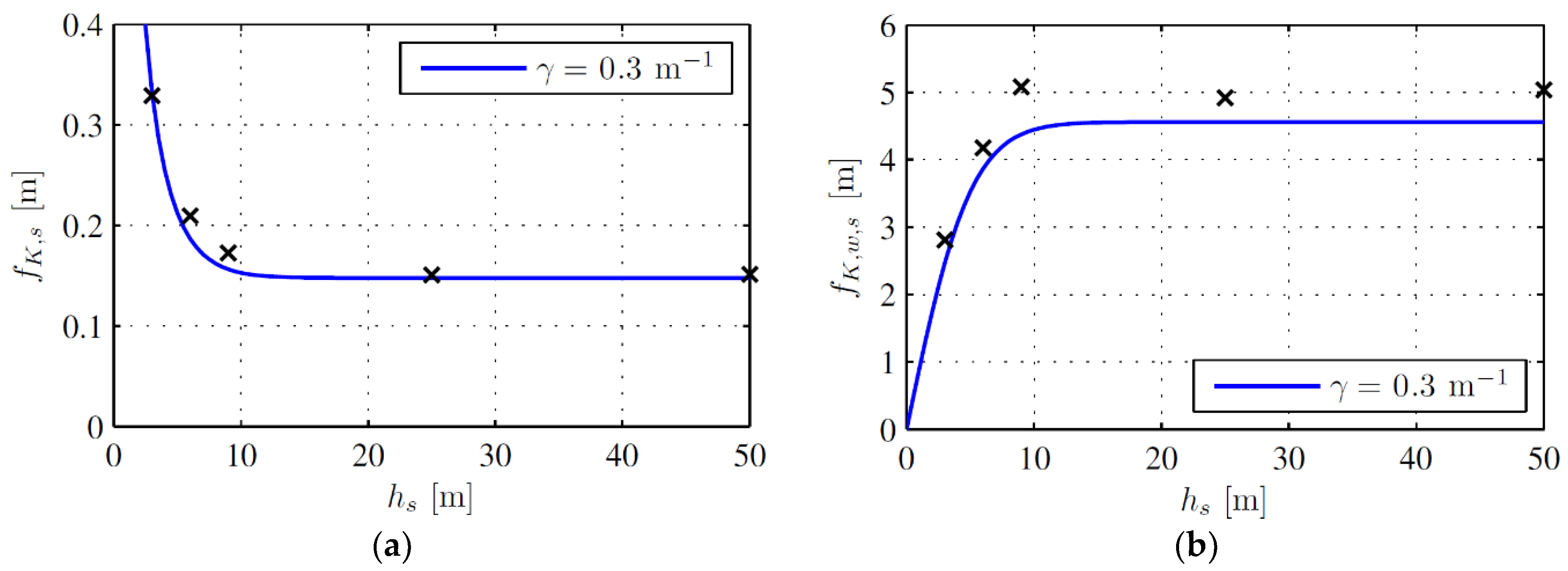
The expressions proposed in Equations (1), (3), (7), (8), (10), (12)–(17) define all the parameters of the DSM from the known properties of the track, with the exception of the angle of stress distribution in the ballast, ${\alpha }_b$, the rate of displacement decrease with depth in the subgrade, $\gamma$, and the rate of absorption due to radiation damping, $c_z$.

To determine the values for these parameters, the expressions above are fitted to the numerical results obtained in the previous sections. Since there are only a few discrete points to fit, a simple norm of the relative difference between the theoretical and numerical results is used.

The first parameter to optimize is ${\alpha }_b$, which must fit both ballast depths, $h_b=0.3 \mathrm{m}$ and $h_b=0.6 \mathrm{m}$. The resulting optimum value for the first set in Table 2 is ${\alpha }_b=49.8$°, and produces an error of $\pm 9\%$, while for the second set in Table 2 it is ${\alpha }_b=47.6$° with an error of $\pm 4\%$. The values are shown in

Table 4. Optimized value of ${\alpha }_b$, $f_{K,b}$ [m] and respective error, optimum values from Table 2.

$\begin{array}{c}{\mathit{h}}_{\mathit{b}}\\ \mathbf{\left[}\mathbf{m}\mathbf{\right]}\end{array}$	Opt. Val.	${\mathit{\alpha }}_{\mathit{b}}\mathbf{=}\mathbf{49.8}$°	Error	Opt. Val.	${\mathit{\alpha }}_{\mathit{b}}\mathbf{=}\mathbf{47.6}$°	Error
	${\mathit{f}}_{\mathit{K}\mathbf{,}\mathit{b}}$	${\mathit{f}}_{\mathit{K}\mathbf{,}\mathit{b}}$		${\mathit{f}}_{\mathit{K}\mathbf{,}\mathit{b}}$	${\mathit{f}}_{\mathit{K}\mathbf{,}\mathit{b}}$
0.3	1.911	2.086	+9%	1.956	2.029	+4%
0.6	1.483	1.344	−9%	1.349	1.302	−4%

.

Using these values of ${\alpha }_b$, it is possible to define the area of the base of the stress cone and proceed to the optimization of $\gamma$ and $f_{K,s}$. The optimum value for the first set in Table 2 is $\gamma =0.268 {\mathrm{m}}^{-1}$, with an error of $f_{K,s}$ from −16% to +18%, and for the second set in Table 2 it is $\gamma =0.324 {\mathrm{m}}^{-1}$, with an error of $f_{K,s}$ from −11% to +15%.

Then, it is possible to use the above determined values of ${\alpha }_b$ and $\gamma$ to compute the shear stiffness of the ballast and the subgrade.

Table 5. Value of $f_{K,w,b}$ [m] and respective error, optimum values from Table 2.

$\begin{array}{c}{\mathit{h}}_{\mathit{b}}\\ \mathbf{\left[}\mathbf{m}\mathbf{\right]}\end{array}$	Opt. Val.	${\mathit{\alpha }}_{\mathit{b}}\mathbf{=}\mathbf{49.8}$°	Error	Opt. Val.	${\mathit{\alpha }}_{\mathit{b}}\mathbf{=}\mathbf{47.6}$°	Error
	${\mathit{f}}_{\mathit{K}\mathbf{,}\mathit{w}\mathbf{,}\mathit{b}}$	${\mathit{f}}_{\mathit{K}\mathbf{,}\mathit{w}\mathbf{,}\mathit{b}}$		${\mathit{f}}_{\mathit{K}\mathbf{,}\mathit{w}\mathbf{,}\mathit{b}}$	${\mathit{f}}_{\mathit{K}\mathbf{,}\mathit{w}\mathbf{,}\mathit{b}}$
0.3	0.250	0.226	−9%	0.109	0.222	+104%
0.6	0.722	0.949	+31%	0.499	0.930	+86%

shows a summary of these results.

It is seen that the error is quite high, nevertheless, this is not very important, because the main shear contribution comes from the foundation. For the subgrade shear stiffness, using the optimized values of ${\alpha }_b$ and $\gamma$, the error of $f_{K,w,s}$ ranges from −9% to +34% for the first set in Table 2 and from −29% to −14% for the second set. Both $f_{K,s}$ and $f_{K,w,s}$ are plotted as a function of $h_s$ in Figure 12, for a rough average of the optimum values of $\gamma =0.3 {\mathrm{m}}^{-1}$.

It can be concluded that the approximation is quite reasonable, especially taking into account that the optimum values of $\gamma$ were obtained only from optimizing of $f_{K,s}$.

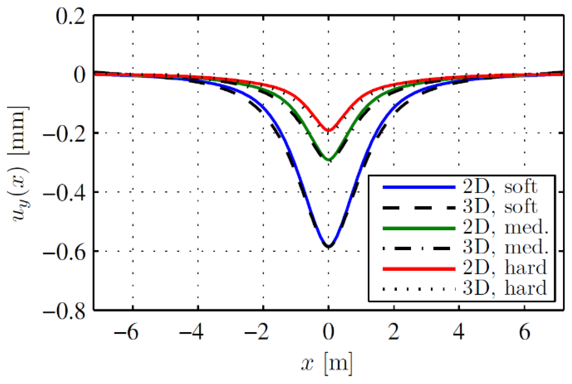
The value of $\mathsf{\Phi }$ obtained for the static solution using these expressions ranges from 3.3% to 14.8% for the first optimization set in Table 2 and from 3.3% to 13.8% for the second set. Vertical displacements for the representative load of 40 kN are compared in Figure 13. It can be concluded that the agreement between DSM with the proposed expressions and the 3D FE model is excellent.

Further, the same comparison must be carried out for the dynamic case. Using the optimum value of ${\alpha }_b$ the error in the proposed expression can be calculated. The results are summarized in

Table 6. Values of the mass and respective error, optimum values from Table 3.

$\begin{array}{c}{\mathit{h}}_{\mathit{b}}\\ \mathbf{\left[}\mathbf{m}\mathbf{\right]}\end{array}$	Opt. Val. $\mathit{v}\mathbf{=}\mathbf{50} \mathbf{m}\mathbf{/}\mathbf{s}$	${\mathit{\alpha }}_{\mathit{b}}\mathbf{=}\mathbf{49.8}$°	Error	Opt. Val. $\mathit{v}\mathbf{=}\mathbf{100} \mathbf{m}\mathbf{/}\mathbf{s}$	${\mathit{\alpha }}_{\mathit{b}}\mathbf{=}\mathbf{49.8}$°	Error
	$\mathit{M}$	$\mathit{M}$		$\mathit{M}$	$\mathit{M}$
0.3	3.283	3.273	−3%	2.469	3.273	+33%
0.6	4.412	4.900	+11%	3.035	4.900	+61%

.

It is clear that the proposed equations provide a good approximation for the lower velocity, but not for the high velocity, for which the optimal mass is 20% to 30% lower, likely because the latter is close to the critical velocity of the track for a soft subgrade. Since the proposed equations do not account for this effect, they work well for low to moderate velocities, but not for high velocities, for which the dynamic amplification is more pronounced.

As for the radiation damping, the numerical optimal values in Table 3 are used to deduce the optimum value of $c_z$. The results are summarized in

Table 7. Optimum values of $c_z$, based on Table 3.

${\mathit{h}}_{\mathit{b}}\mathbf{\left[}\mathbf{m}\mathbf{\right]}$	$\mathit{v}\mathbf{=}\mathbf{50} \mathbf{m}\mathbf{/}\mathbf{s}$	$\mathit{v}\mathbf{=}\mathbf{100} \mathbf{m}\mathbf{/}\mathbf{s}$
0.3	0.393	0.358
0.6	0.347	0.361

. It can be concluded that $c_z=0.4$ is a good recommendation for railway models with properties inside the range studied here.

The value of Φ obtained for the steady-state dynamic solution using these expressions ranges from 8.1% to 13.1% for $v=50 \mathrm{m}/\mathrm{s}$ and from 8.3% to 43.6% for $v=100 \mathrm{m}/\mathrm{s}$. The higher errors are always observed for the soft subgrade ($E_s=50 \mathrm{MPa}$), particularly for $v=100 \mathrm{m}/\mathrm{s}$, as shown in Figure 14, due to the aforementioned dynamic amplification factor due to the critical velocity.

It is of note that the maximum upward and downward displacements for the worst case are relatively close to the ones obtained on the 3D FE model, so the DSM and the proposed expressions provide a reasonable approximation to the rail displacement even when the load is moving with the velocity is close to the velocity of propagation of elastic waves in the soil.

Finally, the results of the DSM are compared with the experimental results published in [46], as was the case for the 3D FE model, using ${\alpha }_b=50$°, $\gamma =0.3 {\mathrm{m}}^{-1}$ and $c_z=0.4$. The vertical displacement obtained in the DSM due to the passage of the full train and a single bogie at 220 km/h is presented in Figure 15.

It can be concluded that the results of the DSM are very close to the ones of the 3D FE model and provide a good approximation of the experimental results. In fact, the results are in better agreement than the ones of the 2D model presented in [46], where the multibody vehicle model was considered, justifying the assumption of moving forces adopted here.

6. Comparison with Other Works

As most of the literature does not present formulas for establishing the model data, as a reference for comparison with other works the model presented in [3] is chosen. In [3], values of $K_b$ and $M_b$ are calculated using ${\alpha }_b=35$° and subgrade stiffness is calculated using the given subgrade modulus ${\overline{K}}_s$. Therefore, the comparison is performed in the following way: the data kept in both models are related to the rail: $EI=6.62 {\mathrm{MNm}}^2$, $m=60.64 \mathrm{kg}/\mathrm{m}$; to the sleepers: $M_{sleep}=125.5 \mathrm{kg}$, $l_s=0.545 \mathrm{m}$, $l_b=0.273 \mathrm{m}$, $l_e=0.95 \mathrm{m}$; to the rail pads: $K_{pad}=65 \mathrm{MN}/\mathrm{m}$, $C_{pad}=75 \mathrm{kNs}/\mathrm{m}$ and to the ballast: $E_b=110 \mathrm{MPa}$, $h_b=0.45 \mathrm{m}$, ${\rho }_b=1800{ \mathrm{kg}/\mathrm{m}}^3$. Ballast vertical and shear damping are neglected as in the final optimization steps.

There is no indication for $E_s$ in [3]. Thus, ${\overline{K}}_s=90 \mathrm{MPa}/\mathrm{m}$ given in [3] is used with the optimized $\gamma =0.3 {\mathrm{m}}^{-1}$ and $h_s=6 \mathrm{m}$, to give $E_s=295.7 \mathrm{MPa}$.

Table 8. Model data summary.

Parameter	Formulas in This Paper	[3]
$K_{w,b}$ [MN/m]	27.3	78.4 *
$K_{w,s}$ [MN/m]	500.9	---
$K_w$ [MN/m]	528.2
$M_b$ [kg]	595.7	531.4
$M_s$ [kg]	3033.6	---
$M$ [kg]	3629.3
$K_b$ [MN/m]	168.27	137.75
$K_f$ [MN/m]	88.8	77.5
$C_f$ [kNs/m]	308	31.15 *

* Means that the value was used without justification.

summarizes the differences in both models.

It is necessary to highlight that values for $K_w$ and $M$, given in Table 8 for the model developed in this paper, are very high due to the contribution from the foundation, as justified by optimizations. In fact, it would be more adequate to include them in a separate foundation layer.

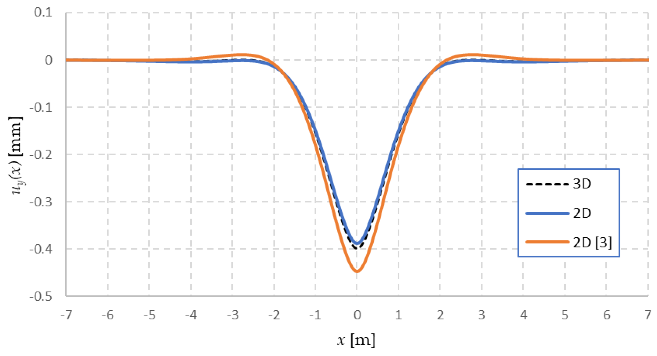
The representative force of 40 kN is used for results comparison, as in previous sections. Static displacement is depicted in Figure 16.

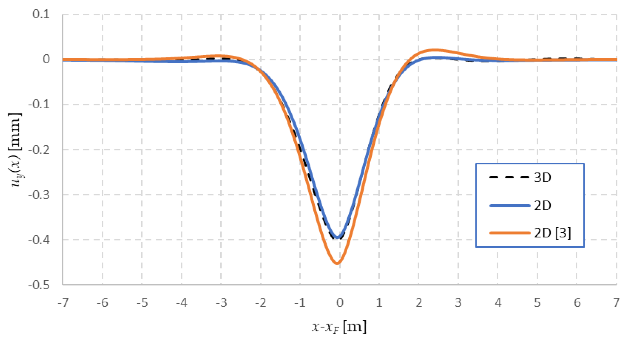
It is seen that the high shear stiffness of the model attenuates the upward displacements which are not present in the 3D FE model. The deflection shape agreement is better for the model presented in this paper. Further, the stabilized steady-state deflection shape is compared to the moving load in Figure 17.

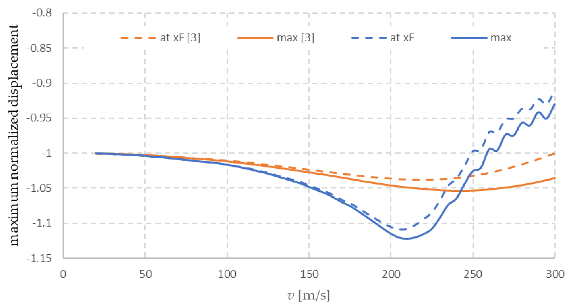
Finally, the maximum displacement values in the absolute value are extracted as a function of velocity. In Figure 18, the maximum value over the structure is plotted together with the value in the load position. The values are normalized by static displacement. The typical fact can be observed that by getting closer to the critical velocity, the maximum downward displacement does not occur at the load position. It is confirmed that the increase in oscillating mass as suggested in this paper makes the prediction of the critical velocity more reasonable, bearing in mind the value of $E_s$. This concludes the comparison.

It was shown that the new formulas led to much better agreement with the 3D FE model, not only in regard to the deflection shape, but also for the prediction of the critical velocity.

7. Conclusions

The present work establishes the validity and the range of applicability of the DSM. It proposes general formulas for identifying all DSM properties without the necessity of calling on experimental results. The formulas proposed are simple and straight-forward to use and avoid the necessity of numerical calibration.

It was shown that the DSM shows a good approximation to the 3D FE model for the whole range of parameters considered—ballast and subgrade depth and the Young moduli. However, since the DSM does not model the elastic wave propagation in the soil, it is less reliable when the load moves at a speed close to the critical velocity. Good agreement was observed up to a speed of 75% of the Rayleigh wave velocity in the subgrade (8%–13% overall error), while at a speed very close to the Rayleigh waves, the error became more significant (18%).

All DSM components can be determined from basic mechanical and geometrical properties, except for three fundamental values, for which the following values were found to provide a good approximation:

• Angle of stress distribution in the ballast: ${\alpha }_b=50$°;
• Rate of displacement reduction with depth in the subgrade: $\gamma =0.3 {\mathrm{m}}^{-1}$;
• Rate of absorption for the radiation damping of the subgrade: $c_z=0.4$.

Regarding the formulas available in the literature, it was concluded that the oscillating mass of the model cannot represent only the dynamically activated ballast mass, but the contribution from the foundation must be added. The same conclusion was taken regarding the shear stiffness of the model: the value determined for the ballast has to be superposed with the contribution coming from the foundation. The shear stiffness of the model is essential for achieving a good agreement. This means that reduced models that are focusing mainly on the vertical dynamic equilibrium and/or are neglecting the dynamically activated mass in the foundation, cannot represent the rail deflection shape accurately within the range of typical track properties even in the subcritical velocity range.