Article

Numerical Assessment of Polynomial Nonlinear State-Space and Nonlinear-Mode Models for Near-Resonant Vibrations

1
Department of Mechanical Engineering, Rice University, Houston, TX 77005, USA
2
Department of Mechanical Engineering, Imperial College, London SW7 2BU, UK
3
Institute for Aircraft Propulsion Systems, University of Stuttgart, 70569 Stuttgart, Germany
4
ETH Zürich, 8092 Zürich, Switzerland
5
Control Systems Technology Group, Eindhoven University of Technology, 5612 AZ Eindhoven, The Netherlands
*
Author to whom correspondence should be addressed.
Vibration 2020, 3(3), 320-342; https://doi.org/10.3390/vibration3030022
Submission received: 25 August 2020 / Revised: 13 September 2020 / Accepted: 14 September 2020 / Published: 18 September 2020
(This article belongs to the Special Issue Data-Driven Modelling of Nonlinear Dynamic Systems)

Abstract

:
In the present article, we follow up our recent work on the experimental assessment of two data-driven nonlinear system identification methodologies. The first methodology constructs a single nonlinear-mode model from periodic vibration data obtained under phase-controlled harmonic excitation. The second methodology constructs a state-space model with polynomial nonlinear terms from vibration data obtained under uncontrolled broadband random excitation. The conclusions drawn from our previous work (experimental) were limited by uncertainties inherent to the specimen, instrumentation, and signal processing. To avoid these uncertainties in the present work, we pursued a completely numerical approach based on synthetic measurement data obtained from simulated experiments. Three benchmarks are considered, which feature geometric, unilateral contact, and dry friction nonlinearity, respectively. As in our previous work, we assessed the prediction accuracy of the identified models with a focus on the regime near a particular resonance. This way, we confirmed our findings on the strengths and weaknesses of the two methodologies and derive several new findings: First, the state-space method struggles even for polynomial nonlinearities if the training data is chaotic. Second, the polynomial state-space models can reach high accuracy only in a rather limited range of vibration levels for systems with non-polynomial nonlinearities. Such cases demonstrate the sensitivity to training data inherent in the method, as model errors are inevitable here. Third, although the excitation does not perfectly isolate the nonlinear mode (exciter-structure interaction, uncontrolled higher harmonics, local instead of distributed excitation), the modal properties are identified with high accuracy.

1. Introduction

The high demand for saving resources and avoiding emissions in recent years has led manufacturers to make increasing use of lightweight design. These components are more sensitive to external loads resulting in vibration regimes where geometric nonlinearities can no longer be neglected [1]. Besides geometric nonlinearities, material behavior and contact interactions are predominant sources of nonlinear force-deformation relations in mechanical systems. In particular, the primary cause of mechanical damping in structural assemblies is usually the nonlinear frictional interactions in joints [2]. In fact, additional joints are deliberately introduced to increase damping, as in the case of dry friction dampers in turbomachinery. Often, linear theory is not sufficient to explain the dynamics in the presence of such nonlinearities, but methods that explicitly account for nonlinearities are required to ensure the proper functioning and safe operation of mechanical systems.
Compared to numerical methods, experimental methods for nonlinear systems are still in their infancy. An important branch of experimental methods are nonlinear system identification techniques [3]. System identification refers to systematically deriving models or extracting information about the system behavior directly from measured data [4]. Although virtual prototypes and numerical simulation find increasing use, the data-driven system identification may be preferred over physics-driven modeling, for instance if the underlying processes are not properly understood or too complicated [5]. Moreover, system identification is commonly used for validating, updating or upgrading physics-based models. The present interest, in particular, is focused on system identification techniques that can be used for the study of mechanical systems with nonlinearities that “perturb” linear resonances in an amplitude-dependent fashion. Common examples of such systems include thin beams, plates, and shells undergoing large amplitude vibrations (see Reference [6] for a relatively recent review); nonlinear vibrations of jointed structures with contact and frictional nonlinearities (see Reference [7] for perspectives); etc.
The last few decades have seen several developments in nonlinear system identification techniques used in structural dynamics. Yet, to date, there is no nonlinear system identification method that can be applied to all systems [3]. An exhaustive literature review is beyond the scope of the present study; for this, we refer to References [4,8]. The present work follows up the experimental campaign reported in References [9,10]. The objective of that campaign was to assess both merits and deficiencies of two representative nonlinear system identification methods which employ fundamentally different training data for the identification: With the first method, a single-nonlinear-mode model is identified from periodic vibration data obtained for controlled harmonic excitation. With the second method, a polynomial nonlinear state-space (PNLSS) model is identified from random broadband training data. As benchmarks, a beam with repelling magnets and a system of two beams with bolted joints were considered. It was found that the identified nonlinear-mode models provided good prediction accuracy near the primary resonance. In reality, of course, no reference data is available for the modal properties. Therefore, it was unclear if the remaining deviations are a methodological deficiency or just a reflection of the system-inherent variability. Moreover, it was found that the identified PNLSS models were highly sensitive to the training data and provided relatively low prediction accuracy. Again, since the true functional form of the nonlinearity is not available in reality, it remains unclear if this is due to a methodological deficiency or a model error. The purpose of the present work was to address these open questions, by resorting to synthetic measurement data obtained from simulated experiments. Only this way, the actual mathematical form of the nonlinearity is known and an unspoiled (noise, system variability, measurement uncertainty) reference for the modal properties becomes available. While these simulated experiments permit a more thorough assessment of the methodologies, one of course loses some of the immediate practical significance which only real experiments can provide.
The rest of the paper is organized as follows: The two system identification methods are briefly described in Section 2. An overview of the benchmarks and the comparison strategy is given in Section 3. The numerical results are presented in Section 4. Finally, conclusions are drawn in Section 5.

2. Description of the Nonlinear System Identification Methods

In this section, the methods for identifying a nonlinear-mode model and a PNLSS model are summarized.

2.1. Identification of a Nonlinear-Mode Model

The concept of normal modes is quintessential to the vibration analysis of linear mechanical systems. Consequently, scientists have explored opportunities to extend this powerful concept to the nonlinear case. The earliest attempts date back to the 1960s [11]; for a thorough review article, the reader is referred to Reference [12]. Nonlinear modes provide insight into the qualitative vibration behavior (e.g., softening/hardening, importance of higher harmonics, energy localization). Under some conditions, the vibration energy is confined to a single nonlinear mode (single-nonlinear-mode theory) [13]. In particular, this is the case if the mechanical system is externally driven near a well-separated primary resonance. This may also be the case under self-excitation [14,15], or combinations of self- and forced excitation [16]. When the vibration is dominated by a single nonlinear mode, the dynamics take place on a two-dimensional invariant manifold in state-space [17,18,19], and the mechanical system behaves like a single-degree-of-freedom oscillator.
In this work, we use the definition of a nonlinear mode in accordance with the Extended Periodic Motion Concept (EPMC) [20]: Consider an autonomous nonlinear mechanical system with the equation of motion M ̲ ̲ q ̲ ¨ + g ̲ ( q ̲ , q ̲ ˙ ) = 0 ̲ , where q ̲ is the vector of generalized coordinates, overdot denotes derivative with respect to time t, M ̲ ̲ is the symmetric and positive-definite mass matrix, and g ̲ is the vector of generalized linear or nonlinear damping and restoring forces. A nonlinear mode is then the family of periodic solutions q ̲ of M ̲ ̲ q ̲ ¨ 2 D ω M ̲ ̲ q ̲ ˙ + g ̲ ( q ̲ , q ̲ ˙ ) = 0 ̲ , that continues the corresponding linear mode to high amplitudes. ω is the fundamental frequency and corresponds to the modal frequency, D is the modal damping ratio, and the Fourier coefficients of the periodic solution are the harmonics of the modal deflection shape. The artificial negative damping term 2 D ω M ̲ ̲ q ̲ ˙ compensates the natural dissipation (in average over a vibration cycle). The EPMC simplifies to the conventional periodic motion concept in the conservative case, and is consistent with the linear case under modal damping [21]. If, at the same time, more than one linear mode contributes strongly to the nonlinear mode, and damping is not light (i.e., D not 1 ), the artificial term will generally distort the modal coupling [20].
Modal analysis denotes the process of determining modal properties, i.e., modal frequency, damping ratio and deflection shapes. The modal analysis in accordance with the EPMC can be carried out computationally using standard methods such as Harmonic Balance or Shooting, or experimentally using feedback control, as, e.g., in the form of phase-resonant testing [22], response-controlled step sine testing [23], or Control-Based Continuation [24,25]. In this work, the method proposed in Reference [22] is used, i.e., the periodic motion is ensured with an appropriate external excitation. This approach generalizes phase-resonant testing, which is well-known for linear systems, to nonlinear non-conservative systems. As was shown in Reference [22], in many cases, a nonlinear mode can be well-isolated with a single-point excitation and requiring only local phase resonance with regard to the fundamental harmonic. This was achieved in Reference [22] using a phase controller, called phase-locked loop (PLL), which adapts the excitation frequency until the desired resonant phase lag is reached. Details of the controller can be found in Reference [22]. By varying the excitation level, the backbone curve of the frequency response is tracked. Once phase resonance is achieved at a given excitation level, the corresponding modal amplitude a, modal frequency ω ( a ) , and fundamental harmonic of the mass-normalized modal deflection shape φ ̲ 1 ( a ) can be recorded. To achieve the mass normalization in experimental practice, the mass-normalized mode shapes obtained by conventional linear modal testing at sufficiently low excitation level can be used [22]. In this numerical study, the mass matrix is available and directly used for mass normalization. The modal damping ratio D ( a ) is determined by the balance between the time-averaged active power provided to the system via the exciter and that dissipated by the system.
Assuming that the structural response is dominated by a single nonlinear mode (single-nonlinear-mode theory), the periodic oscillation can be approximated as
q ̲ ( t ) = a n = 0 H φ ̲ n ( a ) e i n 0 t Ω d t + θ .
Herein, a and θ denote the real-valued modal amplitude and phase, respectively, a φ ̲ n ( a ) e i n θ are the complex Fourier coefficients of the modal deflection shape, and Ω is the generally time-dependent oscillation frequency. The fundamental harmonic of the mode shape is mass-normalized with φ ̲ 1 H M ̲ ̲ φ ̲ 1 = 1 , where H denotes Hermitian transpose. In computational and experimental practice, only a finite number of H Fourier coefficients of the modal deflection shape can be determined. Substituting the ansatz (Equation (1)) into the equation of motion, and requiring orthogonality of the residual with respect to the fundamental harmonic of the nonlinear mode, one obtains the following complex nonlinear first-order ordinary differential equation for a and θ ,
2 i Ω a ˙ + i a θ ˙ + Ω 2 + 2 D a ω a i Ω + ω 2 a a = φ ̲ 1 a H f ̲ ^ 1 e i θ .
f ̲ ^ 1 is the vector of fundamental Fourier coefficients of the imposed external forces. The steady-state limit is simply obtained by setting a ˙ = 0 = θ ˙ , which results in an algebraic equation. The identified modal model will be referred to as the Nonlinear Modal-Reduced Order Model (NM-ROM) henceforth.

2.2. Identification of a PNLSS Model

To obtain a PNLSS model, we use the specific method developed in Reference [26]. This method yields a discrete-time multiple-input-multiple-output state-space model in the form of
x ̲ n + 1 = A ̲ ̲ x ̲ n + B ̲ ̲ u ̲ n + E ̲ ̲ e ̲ ( x ̲ n ) y ̲ n = C ̲ ̲ x ̲ n + D ̲ ̲ u ̲ n ,
where the vectors x ̲ , u ̲ , y ̲ represent the states, inputs, and outputs, respectively. The coefficient matrices A ̲ ̲ , B ̲ ̲ , C ̲ ̲ , D ̲ ̲ describe the underlying linear behavior, as in classical linear system identification [27]. This classical formulation is augmented by the nonlinear term E ̲ ̲ e ̲ ( x ̲ n ) , where e ̲ ( x ̲ n ) contains all monomial combinations of the states of degree 2 and 3, and E ̲ ̲ is the associated coefficient matrix.
The coefficient matrices are determined by numerical optimization. The objective function is the squared difference between measured and simulated output, summed over a given time span [28]. In this numerical study, synthetic data obtained by a simulated experiment is used as measured output for this training. As input, multisine signals that have a discrete frequency spectrum with prescribed magnitudes, random phases, and a constant magnitude over a certain frequency band and zero magnitude otherwise are used [29]. These so-called general purpose multisine signals, also known as random-phase Schroeder Multisine signals with a flat amplitude spectrum [27], can be expressed mathematically as
u ( t ) = k = 1 F A F / 2 cos ( 2 π f k t + ϕ k ) ϕ k U ( 0 , 2 π ) ,
where f k are the discrete frequency components required in the spectrum; ϕ k are the phases (generated as uniformly distributed random variables in ( 0 , 2 π ) (denoted by U ( 0 , 2 π ) in the above); A is the required signal root-mean-square (RMS) amplitude; F is the number of frequency components. The discrete frequency components are chosen as all the frequency components in a given range separated by the given frequency resolution ( f k = F m i n + k Δ f , with F m i n , Δ f , and F m i n + F Δ f being the minimum frequency, frequency resolution, and maximum frequency, respectively). The signals are constructed in the time-domain using the formula in Equation (4) for the studies presently. The actual excitation signal consists of several repetitions (called blocks) of multisine realization for each amplitude. Transients decay during the first few blocks, and are discarded for the identification. To apply the method also to transient/non-periodic responses, the initial conditions can be identified, as well. The identified model is referred to as the polynomial nonlinear state-space (PNLSS) model henceforth.
By comparing the design of the two system identification methods, one may notice that the modal approach relies on a more involved excitation strategy (phase control), so the tests are more difficult to set up. On the other hand, the model properties can be easily obtained from the measured data for this approach. In contrast, the training data for the PNLSS model is more easy to gather, since no control is needed. On the other hand, the step to obtain model properties from measured data is more involved, as this requires solving a nonlinear optimization problem with a possibly large number of design variables (in general all elements of the coefficient matrices). This step is computationally demanding and requires an appropriate initial guess. As initial guess, the Best Linear Approximation is used, i.e., the best fit of the model in Equation (3) without the nonlinear terms, if not otherwise specified [29].

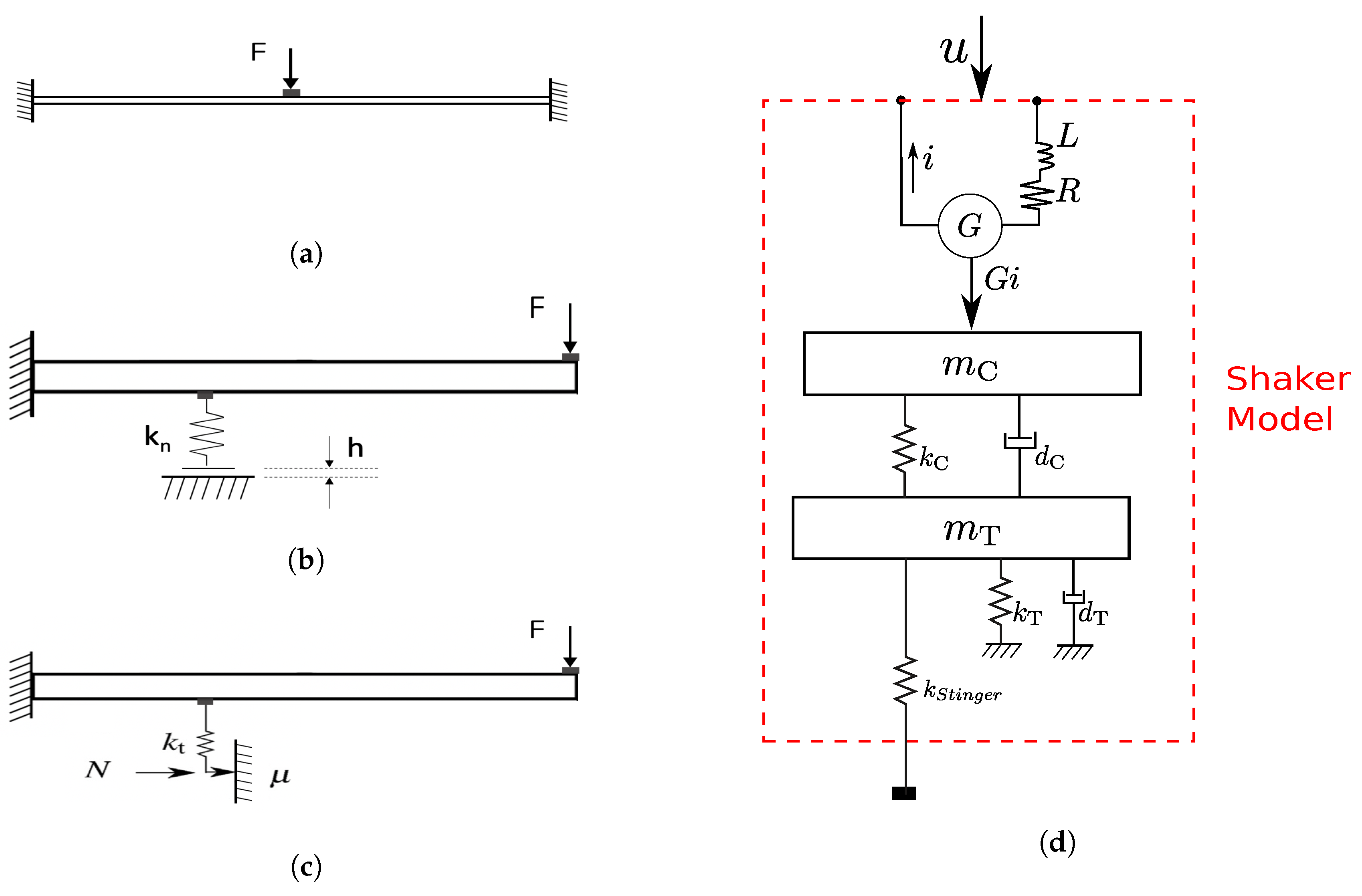
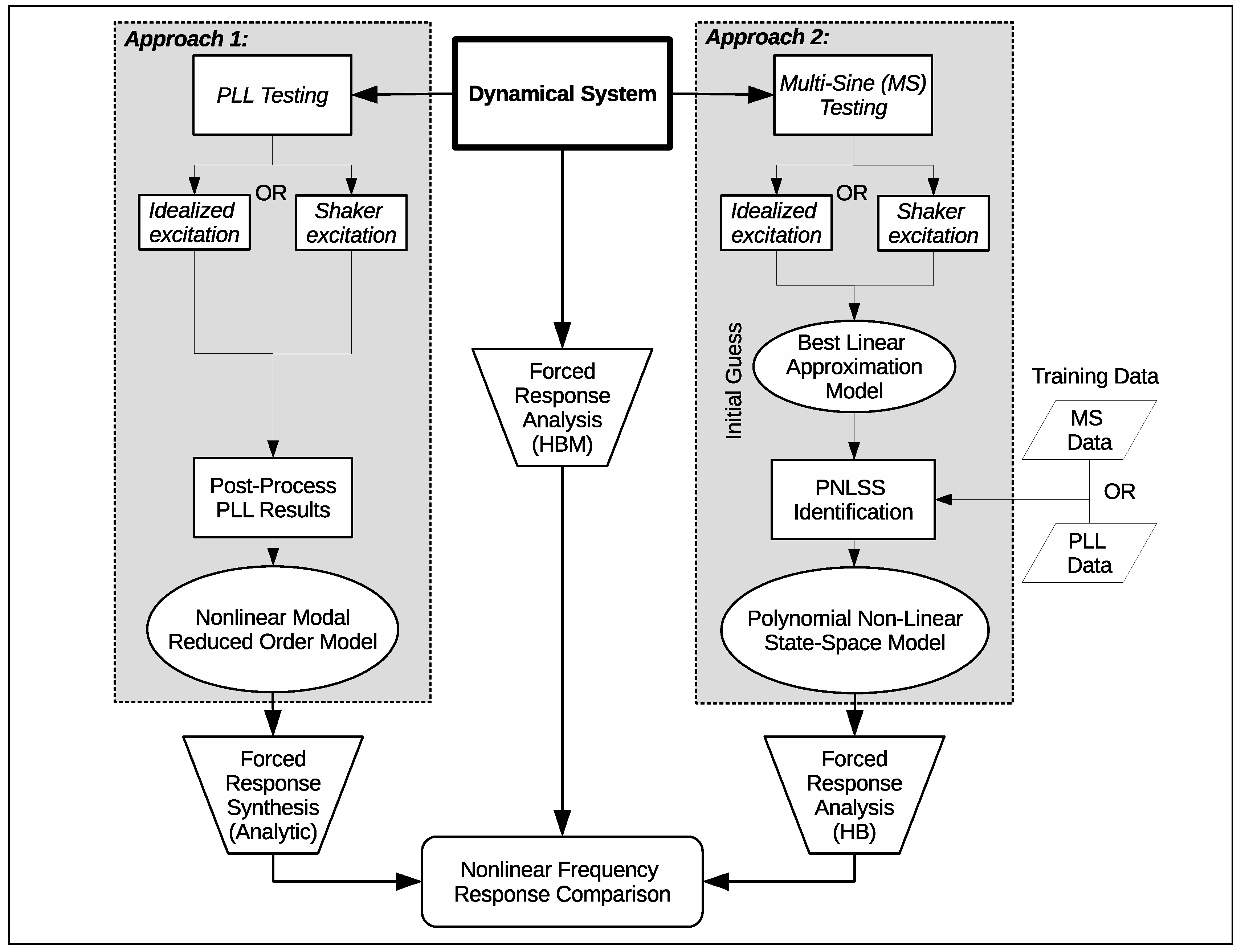
3. Overview of Benchmarks and Comparison Strategy

The benchmarks used in this paper span different types of nonlinearities practically encountered, ranging from stiffness nonlinearities (occurring in geometrically nonlinear applications) to contact nonlinearities involving unilateral contact-separation, as well as hysteretic dry friction nonlinearity. The first benchmark is a geometrically nonlinear clamped-clamped thin beam model undergoing large (in relation to thickness) deformations (Figure 1a). The second and third benchmarks, as shown in Figure 1b,c, are clamped-free Euler-Bernoulli beams with dry-friction nonlinearity (modeled using a Jenkins element) and with a unilateral contact nonlinearity (modeled with a unilateral spring), respectively. Detailed parametric descriptions are provided in the results section. For the multisine signal generation, the amplitude levels are chosen manually so as to ensure that the resulting responses provide a good picture of the nonlinear phenomena characteristic of each system.
A key aspect of this study is to develop an understanding of the influence of a practical experimental setup on the identified models. In particular, the effect of exciter-structure interaction is analyzed. In this numerical study, this can be easily achieved by including a shaker model or replacing it with a unity gain (idealized excitation). Exciter-structure interaction is known to lead to a near-resonant force drop and the occurrence of higher harmonics in the applied force for purely harmonic input to the shaker. The model and the parameters of the electrodynamic excitation system (referred to as the shaker in the rest of the paper) employed in this paper (Figure 1d) follows Reference [22] and represents the Brüel & Kjær Vibration Exciter 4808 as identified in Reference [30]. Parameters used in the model are specified in Table 1.
For the PLL, a PID controller is used, the parameters of which were heuristically tuned in order to achieve robust behavior. For the current study, the controller and the benchmark system are implemented in Simulink. Time integration is carried out using the Dormand-Prince algorithm [31] (an adaptive Runge-Kutta 4-5 explicit time stepper). For the PNLSS model identification, unless mentioned otherwise, a state-space model with two internal states, one input and one output, with all monomial combinations of the states of order up to 3 is used. The restriction of the nonlinearities up to order 3 is used to ensure that the computational costs for the PNLSS identification is not significantly larger than that for the NM-ROM identification (since the number of nonlinear terms grows quickly with the order of the nonlinearities).
Figure 2 outlines the methodology followed for the comparisons in the current study. As mentioned before, the quality of the identified models is assessed by determining their ability to predict the frequency response near a particular primary resonance. To this end, the periodic vibration response to harmonic external forcing is determined, for the near-resonant frequency range, at various force levels. The forcing is a concentrated load applied to a certain location. To obtain the reference or “true” solution, the mathematical model of the benchmark system is analyzed using the high-order harmonic balance method implemented in the open source MATLAB tool NLvib [32]. To compute the frequency response of the PNLSS model in Equation (3), harmonic balance is used, as well. The frequency response of the modal model is determined by considering the steady state form of Equation (2), taking the magnitude on both sides, and solving for the frequency Ω as function of the amplitude a in closed form.

4. Results

4.1. Geometrically Nonlinear Beam/Duffing Oscillator

The model of the clamped-clamped beam is truncated to the lowest-frequency bending mode of the linearized system, which yields an equation of motion equivalent to the Duffing oscillator:
q ¨ 1 + 2 D 1 lin ω 1 lin q ˙ 1 + ( ω 1 lin ) 2 q 1 + b 111 ( 1 ) q 1 3 = F ( t ) ϕ 1 ( / 2 ) , with b 111 ( 1 ) = E A 2 0 ϕ 1 ϕ 1 d x 0 ϕ 1 ϕ 1 d x .
Herein, ϕ 1 ( x ) is the mass-normalized deflection shape, ω 1 lin is the natural frequency and q 1 is the modal amplitude, each associated with the lowest-frequency bending mode of the linearized system. Prime denotes derivative with respect to the axial coordinate x. Formally, Equation (5) can be derived by a Galerkin projection of the approximate continuum beam equations onto this linear mode (second-order theory with respect to transverse displacement, see Reference [33]). The length of the beam is = 140 mm , the cross section area A is 8 mm × 1 mm , the Young’s modulus and density are E = 200 GPa and 7830 kg m 3 , respectively. A concentrated load F ( t ) is applied at the beam’s center. The modal damping is set to D 1 lin = 0.0114 (This value was set based on experience, which indicates that a modal damping of around 1% is a common order of magnitude for such structures.).

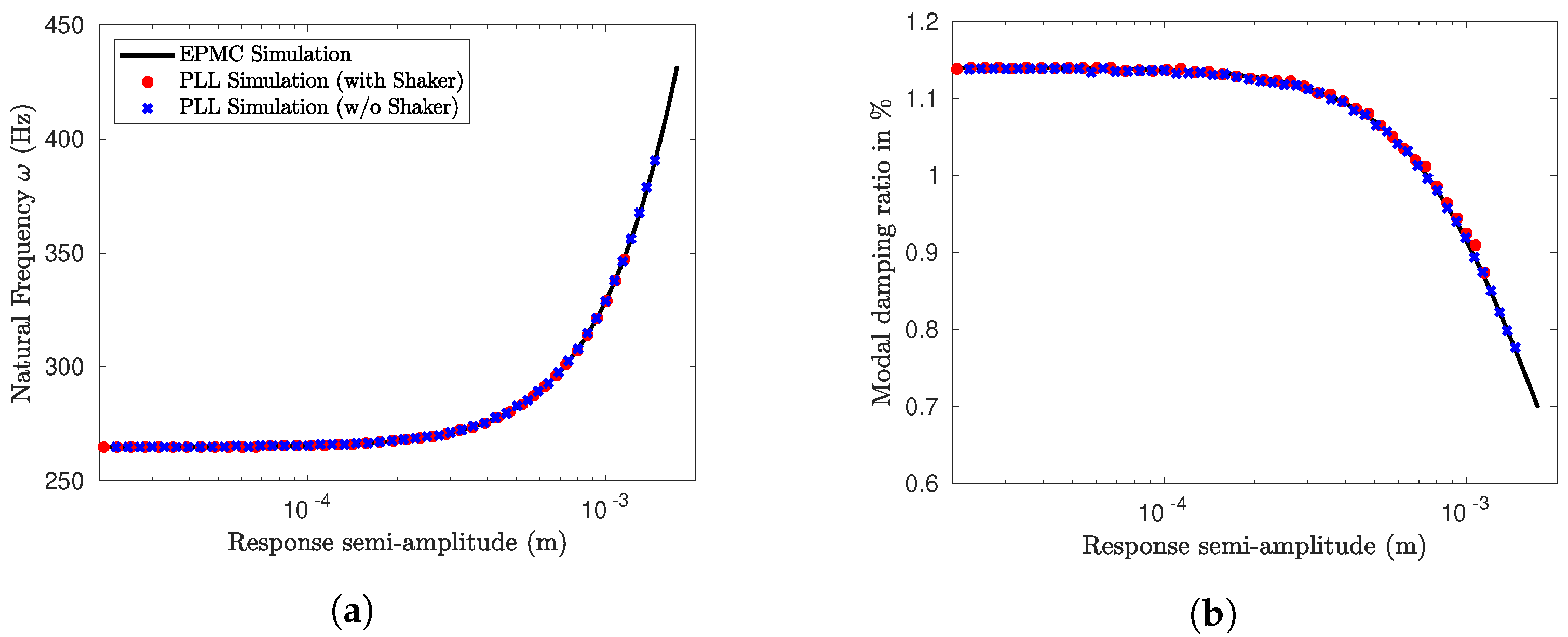
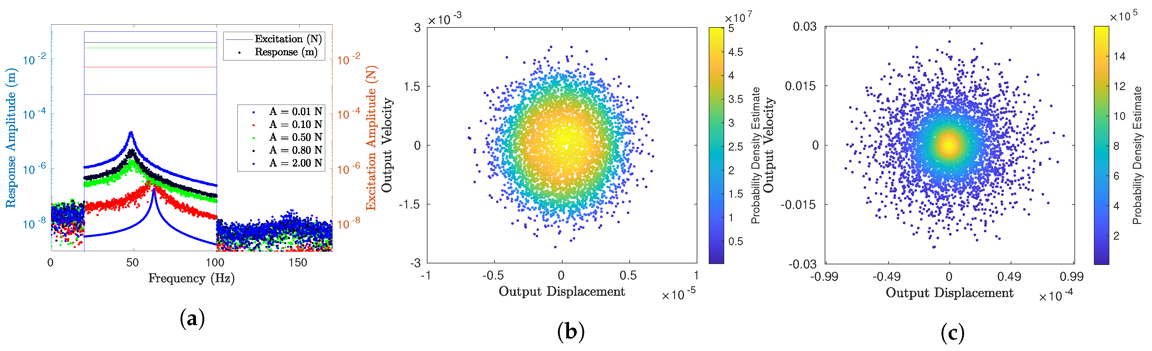
4.1.1. Effect of Excitation Imperfections on the Identified Modal Properties

Recall that, according to the EPMC, the system is driven by negative mass-proportional viscous damping. This self-excitation is therefore distributed and contains higher harmonics in accordance with the vibration response. The nonlinear modal testing proposed in Reference [22] seeks to approximate this by a single-point single-harmonic phase-resonant external forcing (implemented via a PLL). Consequently, the actual periodic vibration state for a given vibration level generally deviates, which may affect the extracted modal properties. The amplitude-dependent natural frequency and modal damping ratio are depicted in Figure 3 both for the theoretical reference (EPMC) and the PLL testing. Two cases are distinguished for the PLL testing, one with and one without exciter-structure interaction. It can be seen that the modal properties obtained via PLL testing are in excellent agreement with the theoretical reference, both in the case with and without shaker.

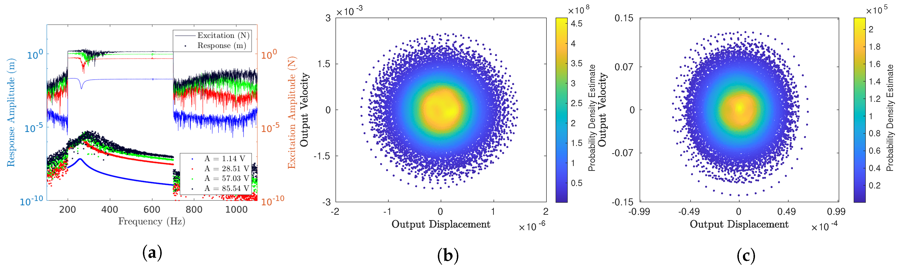
4.1.2. Effect of Exciter-Structure Interaction on the Training Data for the PNLSS Models

For the state-space model in Equation (3), the load F ( t ) is used as input and the transverse displacement at the beam’s center ϕ 1 ( / 2 ) q 1 ( t ) is used as output,
u ( t ) = F ( t ) , y ( t ) = ϕ 1 ( / 2 ) q 1 ( t ) .
The natural frequency of the linearized system is around 265 Hz (Figure 3a). To train the PNLSS model, multisine input is generated in a frequency band between 200 Hz and 700 Hz with a frequency resolution of 0.5 Hz, sampled at 4096 Hz. Two configurations are considered, one where the excitation force F ( t ) is directly prescribed, and one where the voltage input to the shaker is prescribed. In the latter case, the applied force F ( t ) is a result of the harmonic input to the shaker and the exciter-structure interaction. The frequency spectra of the applied force F ( t ) and the output are depicted in Figure 4a and Figure 5a, respectively, for four different excitation levels. The excitation amplitude A is defined as the root-mean-square (RMS) value in each case. While the force magnitude is constant within the specified frequency band by design in Figure 4a, one can see the well-known resonant force drop in the case with a shaker in Figure 5a. The voltage levels were set such that the corresponding off-resonant force levels were similar to the force levels prescribed in the case without shaker.
In the presence of a model error, i.e., if the benchmark system is not a polynomial (of the order assumed in Equation (3)), the identified PNLSS model will be sensitive to the training data. In particular, the model can be expected to be useful and accurate only if the response is in a similar range as the training data. It is, therefore, interesting to gauge the spread of the response in terms of range and distribution. This is done in the state-space diagrams in Figure 4b,c (without shaker) and in Figure 5b,c (with shaker), for two different excitation levels. Note that, in the case of the Duffing oscillator, the state-space dimension is two, such that the state vectors can be depicted completely in these figures. The distribution is illustrated by coloring the point cloud by a Gaussian kernel density estimator. The exciter-structure interaction apparently affects not only the frequency spectra but also the spread of the training data within the state-space. This does not necessarily affect the quality of the identified models, as discussed later.

4.1.3. Inability to Identify an Accurate PNLSS Model in the Case of Chaotic Training Data

An important reason why the Duffing oscillator is an interesting benchmark is that the nonlinearity is of polynomial form. Therefore, one may expect that a PNLSS model with appropriate parameters exactly matches the dynamics of the Duffing oscillator, and a suitable optimization algorithm should be able to find a set of appropriate parameters, up to some numerical tolerance. To the authors’ surprise, this was not always the case. The simple reason for this is that nonlinear systems have sensitive dependence on initial conditions and model parameters in the chaotic regime. A perfect agreement between an identified PNLSS model and the benchmark system cannot be expected in this case due to inevitable perturbations. These perturbations are caused, in particular, by the finite numerical tolerance of the optimization algorithm, the finite sampling rate in the discrete-time representation of the PNLSS model, and the finite step size of the numerical integrator used to simulate the continuous-time representation of the Duffing oscillator. Moreover, as the response is non-periodic, the initial conditions need to be identified simultaneously, as well, which further increases the sensitive dependence of the response on the unknown parameters.
The above described problem is illustrated in Figure 6, where the response of the Duffing oscillator to multisine forcing is depicted (training data), along with the residual of the best linear approximation and the identified PNLSS model. For the lower excitation level, the residual of the PNLSS model is negligible, indicating that appropriate parameters were found such that the PNLSS model matches the Duffing oscillator in a numerically exact way. It should be noted that the response is clearly in the nonlinear regime, which can be easily deduced from the large error made by the BLA. For the higher excitation level, in contrast, the identified PNLSS model yields a large residual. The Lyapunov exponents were estimated based on the technique proposed in Reference [34], and the results are listed in Table 2. Indeed, a positive Lyapunov exponent is obtained for the highest excitation level ( 0.75 N), which confirms that neighboring trajectories exponentially diverge. This leads to large deviations between PNLSS model and Duffing oscillator, regardless of the parameters of the PNLSS model. Consequently, the optimization algorithm cannot distinguish between a poor set of parameters, which would yield a large error also in a regular response regime, and a good set of parameters, which would yield a perfect match in a regular regime. This renders the optimization problem ill-posed and, of course, will have an effect on the identified PNLSS models’ ability to predict the near-resonant frequency response, as discussed in the next subsection.

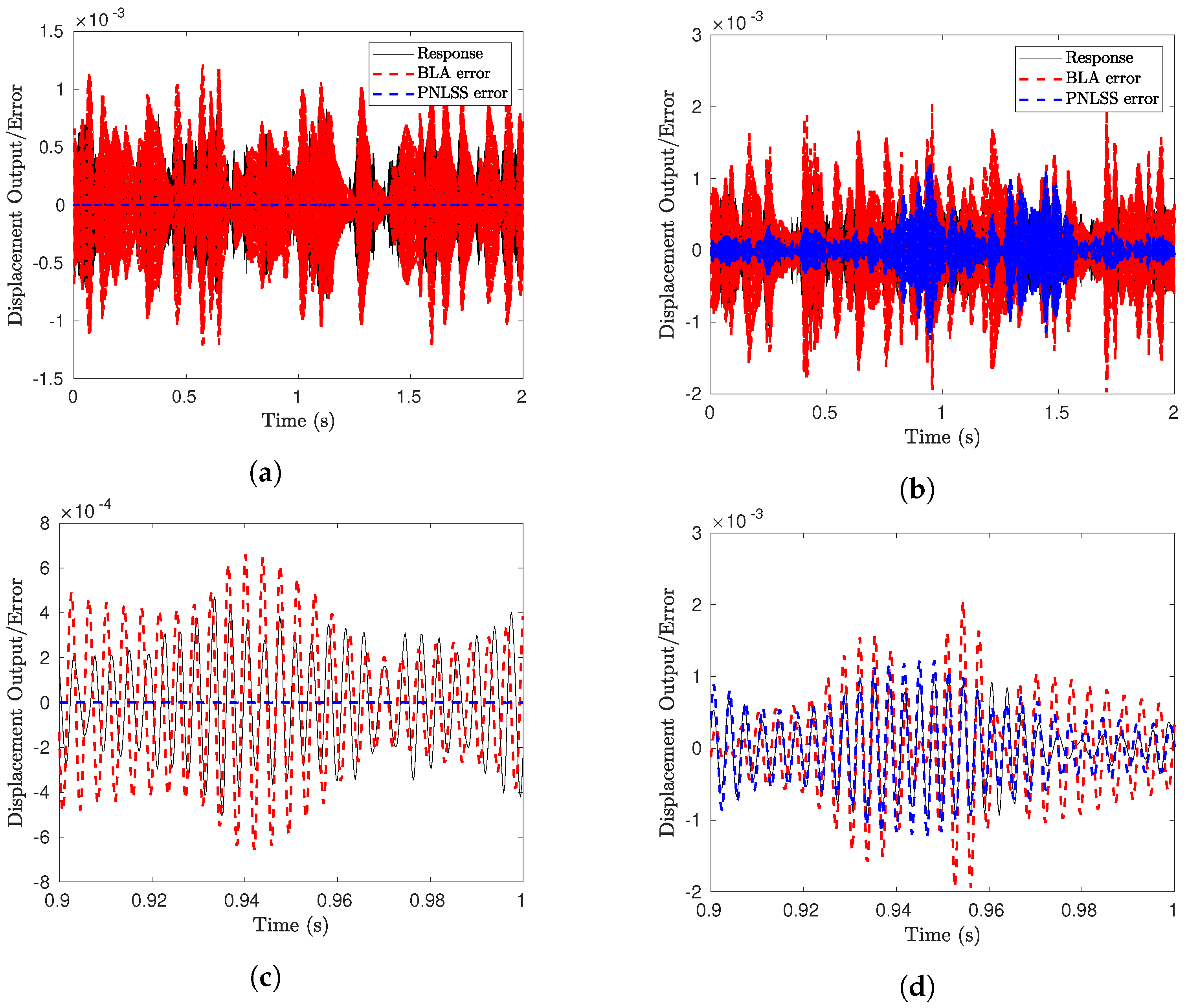
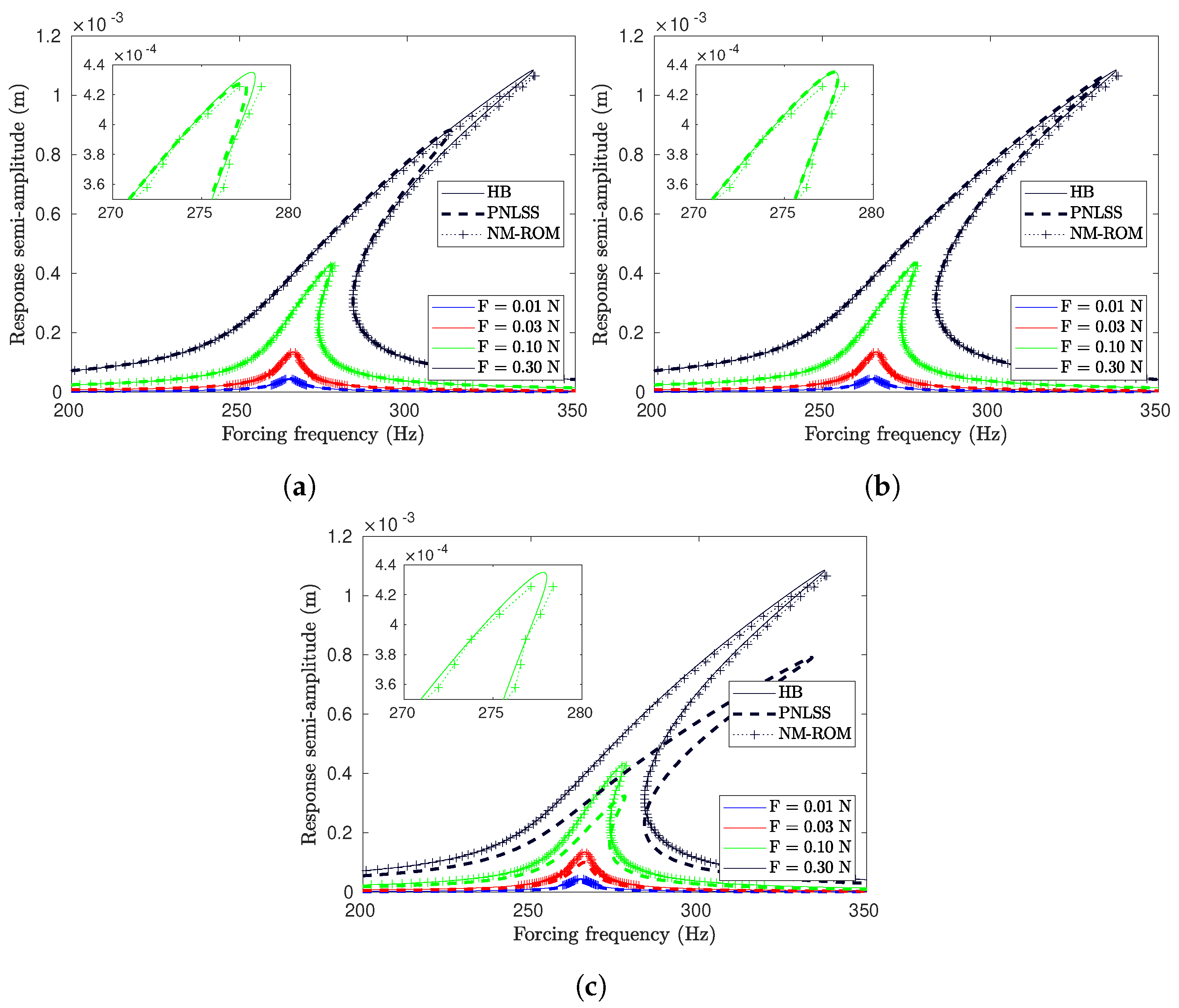
4.1.4. Assessment of the Prediction Accuracy

To assess the quality of the identified models, their ability to predict the near-resonant frequency response is investigated. The results are presented in Figure 7 and Figure 8 for the case of identification without and with shaker, respectively. In the different sub-figures, the results are shown for the PNLSS models obtained for different excitation levels. The results obtained by the NM-ROM and the benchmark are the same in all sub-figures.
As can be expected from the high accuracy of the modal properties in spite of the imperfect excitation (Figure 3), the identified NM-ROM provides high accuracy for identification in the configurations both with and without shaker. A slight deviation is seen for very large response levels. Here, the higher harmonics are pronounced. Even if the NM-ROM is fed directly by the theoretical EPMC results, such an inaccuracy is expected in this regime. This is the price to pay for the simplified projection involving the fundamental harmonic only, which is the key to expressing the nonlinear terms in closed form within the NM-ROM [35].
By comparing the respective sub-figures in Figure 7 and Figure 8, one can notice that the performance of the identified PNLSS model is not significantly affected by the presence of the shaker. It should be emphasized that, in either case, the applied force F ( t ) is considered as input, and thus the shaker behavior is not part of the PNLSS model. The accuracy of the PNLSS model is excellent if it is trained at the intermediate excitation level. The poor performance of the PNLSS model trained at the highest excitation level is due to the ill-posed identification problem in the chaotic regime, as explained earlier. If the PNLSS model is trained at the two depicted lower excitation levels, the training data does not cover the near-resonant response level attained for the higher excitation levels: For training at 0.01 N and 0.5 N excitation level, the displacement training data does not exceed 10 6 m (Figure 4b) and 5 · 10 5 m (Figure 4c), respectively, whereas the resonant response exceeds 10 3 m (Figure 7). Therefore, the nonlinear terms within the PNLSS model are said to be extrapolated. Extrapolating PNLSS models is generally not good practice. In the particular case of the Duffing oscillator, however, there is no systematic model error, and thus the extrapolation does not necessarily lead to poor accuracy. This is confirmed by the great performance of the PNLSS model trained at 0.5 N excitation level (Figure 7b). In contrast, the accuracy of the PNLSS model is only moderate if it is trained at 0.01 N excitation level (Figure 7a). Apparently, the effect of the nonlinear terms is not sufficiently represented in the training data obtained for this excitation level. Consequently, the optimization problem is ill-posed with regard to the coefficients of the nonlinear terms, which explains the lower accuracy encountered in the strongly nonlinear response regime.

4.2. Beam with an Elastic-Dry Friction Contact

The second benchmark is a clamped-free beam with an elastic dry friction element (Figure 1c). The beam is excited at its free end, where the displacement response is also observed. The dimensions of the beam are set as 0.7 m × 0.03 m × 0.03 m , and the Young’s Modulus and density are 185 GPa and 7830 kg m 3 , respectively. The cantilevered beam is discretized using seven standard Euler-Bernoulli finite elements. The friction element is attached to the transverse displacement degree of freedom of the 4th node from the clamped end (coordinate x 4 ). The equations of motion may be expressed as
M ̲ ̲ x ̲ ¨ + D ̲ ̲ x ̲ ˙ + K ̲ ̲ x ̲ + w ̲ f frict = e ̲ F F ( t ) , with x ̲ = [ x 1 , θ 1 , , x N , θ N ] T , w ̲ = 0 0 0 0 0 0 1 0 0 0 T ,
e ̲ F = 0 1 0 T .
Herein, the coordinates x i and θ i denote the transverse displacement and rotation of the ith node (nodal DoFs of the Euler-Bernoulli model), and w ̲ is the unity vector where the element associated with x 4 is equal to one. The hysteretic dry friction force is governed by the differential law
d f frict = k t d x 4 if f frict + k t d x 4 < μ N 0 otherwise .
The tangential stiffness is set to k t = 1.3 × 10 6 N / m and the slip force is set to μ N = 1 N . Proportional damping was introduced as D ̲ ̲ = α M ̲ ̲ + β K ̲ ̲ , wherein the coefficients α and β are set such that the first two modes of the system, when the frictional element is “stuck”, have damping ratios of 0.8% and 0.2%, respectively.

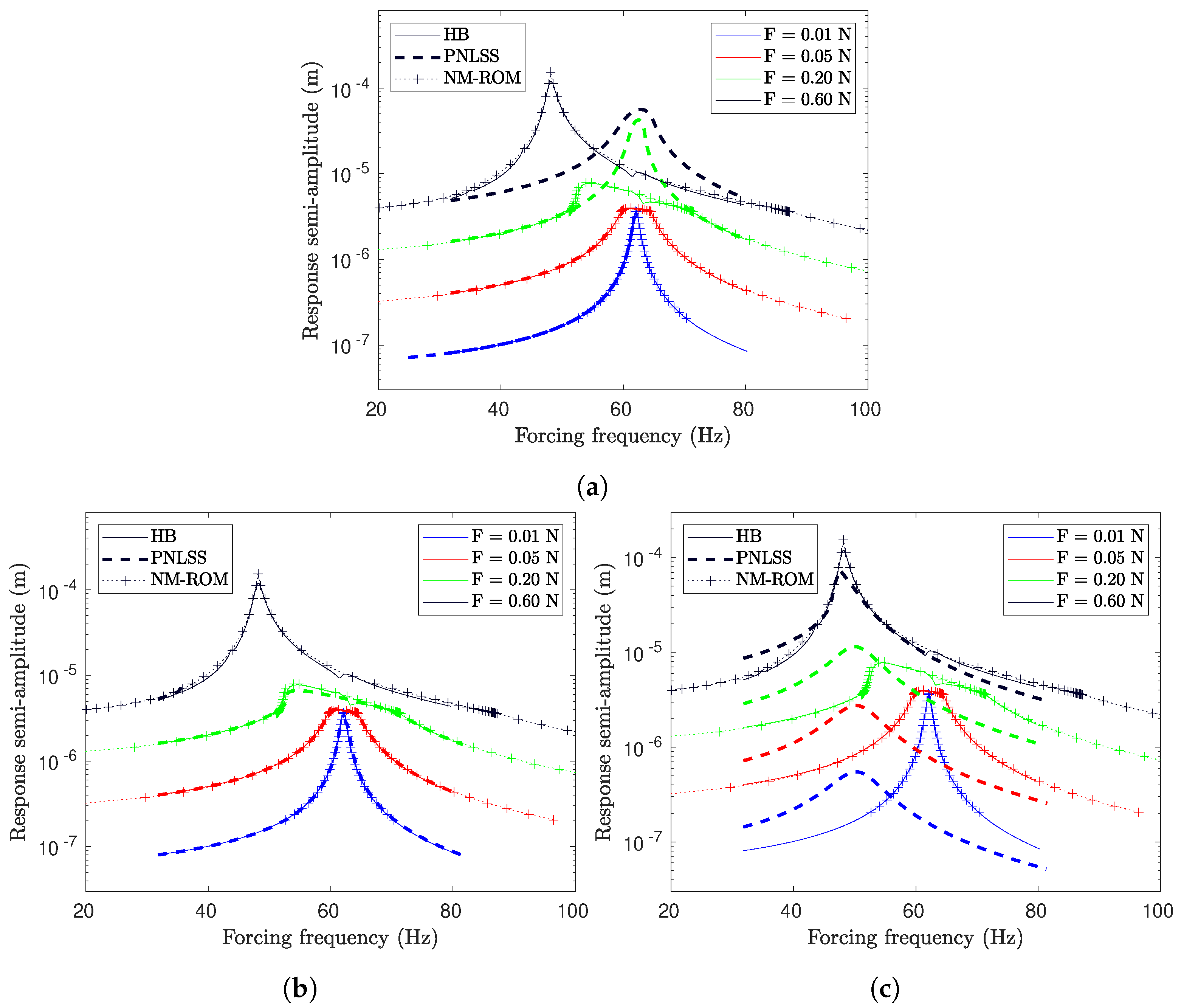
4.2.1. Effect of Excitation Imperfections on the Identified Modal Properties

The amplitude-dependent modal properties of the considered lowest-frequency bending mode are depicted in Figure 9. The softening and nonlinear damping behavior typical for elastic dry friction can be seen. For small vibrations, the friction element sticks, and thus only acts as spring, without providing any damping. For larger vibrations, the sliding phases decrease the equivalent stiffness and increase the dissipated energy. For very large vibrations, the limited friction force (maximum magnitude μ N ) becomes negligible in relation to the elastic and inertia forces, such that the equivalent damping and stiffness of the friction element asymptotically approach zero. Again, for this benchmark, the modal properties obtained by PLL testing are in excellent agreement with the EPMC reference, both in the case with and without shaker.

4.2.2. Identification of the PNLSS Models

For the PNLSS model, the applied force is used as input, and the tip displacement is used as output:
u ( t ) = F ( t ) , y ( t ) = x N ( t ) .
Recognizing that the nonlinearity in the system consists of a hysteretic component, the state-space dimension used for the PNLSS model was set to three. The rationale behind this comes from the way most generalized hysteretic models can be represented: in “rate form”, i.e., in the form of relationships governing the rate of change of the nonlinear force (see dynamic friction models in Reference [36], discussions on the Duhem model of hysteresis in Reference [37], etc.). Mathematically, such a representation of a hysteretic nonlinearity requires the inclusion of first-order dynamics in addition to the second order dynamics governing the oscillatory system. In the near-resonant condition, a state-space dimension of three (two for the oscillation, one for the hysteresis) is considered to be the smallest number of states necessary to represent the system. Discussions pertaining to PNLSS identification of a hysteretic system may also be found in Reference [38] where the performances of two- and three-state models are compared and discussed. As can be seen from Figure 9, the considered natural frequency is in the range of 45–63 Hz. The multisine signals for the training are designed to have an active frequency band of 20–100 Hz, with a frequency resolution of 0.1 Hz and sampled at a frequency of 4096 Hz for eight periods.
The excitation and response frequency spectra, as well as the spread of the response for two excitation levels are shown in Figure 10, in the format as in the previous section. The response spectrum reflects the softening and nonlinear damping behavior seen also in Figure 9. As in the case of the Duffing oscillator, the exciter-structure interaction had an effect on the training data (resonant force drop), but not the performance of the PNLSS models. The results are not depicted for brevity.

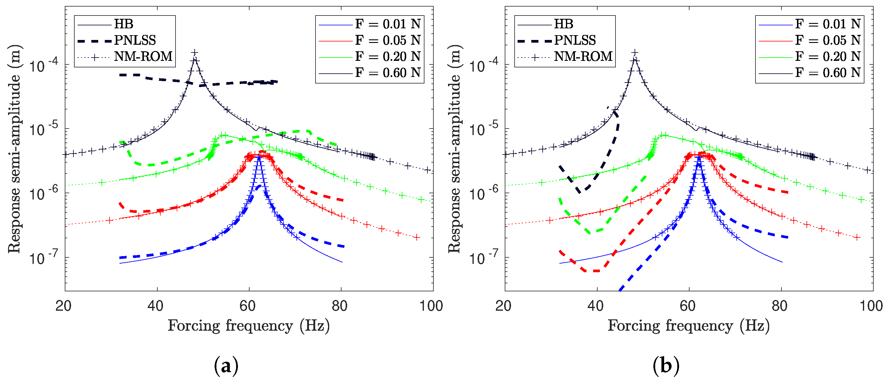
4.2.3. Assessment of the Prediction Accuracy

The quality of the identified NM-ROM and PNLSS models is assessed as for the previous benchmark. The results are depicted in Figure 11.
The NM-ROM provides excellent accuracy for all levels of the harmonic forcing, with one exception: At the highest two force levels, a small secondary peak occurs in the amplitude-frequency curve, not far from the natural frequency under sticking conditions. This singular feature is caused by a nonlinear modal interaction. The phenomenon is not very pronounced as the frictional damping mitigates the energy transfer between the participating modes. Of course, a nonlinear modal interaction cannot be reproduced by a single nonlinear mode only. Therefore, the NM-ROM fails to predict the singular feature attributed to the modal interaction.
Given that the mathematical form of the nonlinearity, a non-smooth hysteretic law, is far from a third-order polynomial, the PNLSS model achieves remarkable accuracy in some cases. In particular, the agreement for the lowest three levels of the harmonic forcing is excellent if the PNLSS model is trained with multisines at 0.10 N RMS level. For the highest force level, however, we did not find a continuous path of real-valued solutions with this model. As expected, the region of validity is dictated by the spread of the training data. When the PNLSS model is trained at 0.01 N, the friction element is mainly sticking, such that the PNLSS model extrapolates this quasi-linear behavior to high response levels. Similarly, when the PNLSS model is trained at 0.80 N, the friction element is mainly sliding, such that the PNLSS model mainly reflects this quasi-linear limit state. In principle, a PNLSS model should be able to represent nonlinear modal interactions. However, we did not succeed in finding a PNLSS model that captures the secondary resonance peak for this benchmark.

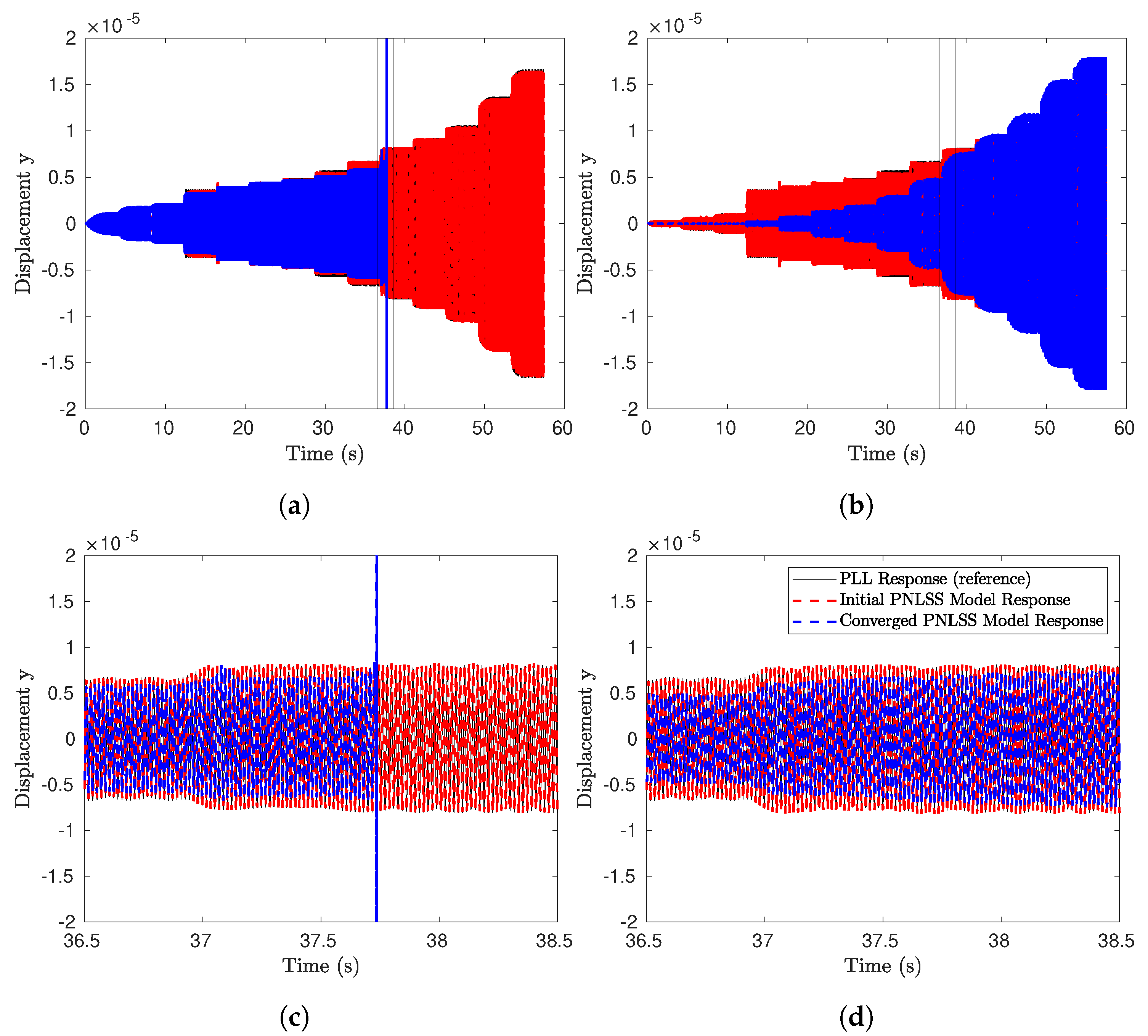
4.2.4. Training the PNLSS Model with PLL Testing Data and Its Effect on the Prediction Accuracy

It should be emphasized that the use of multisines for the training of PNLSS models is a common option, but not the only one. Indeed, a strength of this technique is that quite generic input-output data can be used for the training. The random broadband character of multisines is quite different from the purely harmonic input used for the comparative assessment. In contrast, the measurement data used to identify the nonlinear-mode model is obtained for harmonic input. One could therefore argue that the comparison between NM-ROM and PNLSS models is unfair. To analyze if the assessment is biased by the different data basis for the identification (or training), we trained PNLSS models directly with the input-output data obtained during PLL testing. One can generally say that the optimization problem formulated to identify a PNLSS model is a tough one. The objective function may have numerous local minima, making the converged PNLSS model dependent on the initial guess. As initial guess, we used the PNLSS model identified for multisine input at different levels. Figure 12 shows the output (displacement response) gathered during the simulated PLL testing, the response of the initial PNLSS model and the converged PNLSS model (after training on the PLL data).
One would expect that the optimization algorithm yields PNLSS models that represent the PLL data much better. However, the optimization algorithm did not properly converge when initialized with the PNLSS model trained for 0.1 N. This failure was found to be related to the identified models becoming unstable for the given inputs. One such case is depicted in Figure 12a, wherein the optimization was continued in spite of the instability warnings just for visualizing the unstable model. In addition, when initialized with the PNLSS model trained for 0.8 N, the response does not look closer to the reference after the optimization.
As one may expect from the unsuccessful training, the PNLSS models trained with PLL data yield lower accuracy as compared with the initial ones (trained with multisines of respective level), see Figure 13 and compare with Figure 11b,c.

4.3. Beam with Unilateral Contact

For the final benchmark, the friction element is replaced by a unilateral spring of stiffness k n = 1.3 × 10 6 N / m and initial clearance h = 1 mm (Figure 1b). The beam’s geometric and material properties remain unchanged. The coefficients for the proportional damping model are specified such that the two lowest-frequency normal modes of the linear system with spring k n attached have a damping factor of 0.8%. For computational efficiency, the model order was reduced using the Hurty/Craig-Bampton method [39,40], where the displacement at the unilateral spring, x 4 , was specified as interface coordinate, and two fixed-interface normal modes were retained. For consistency, the reduced model is used both as reference and to gather the data for the identification.

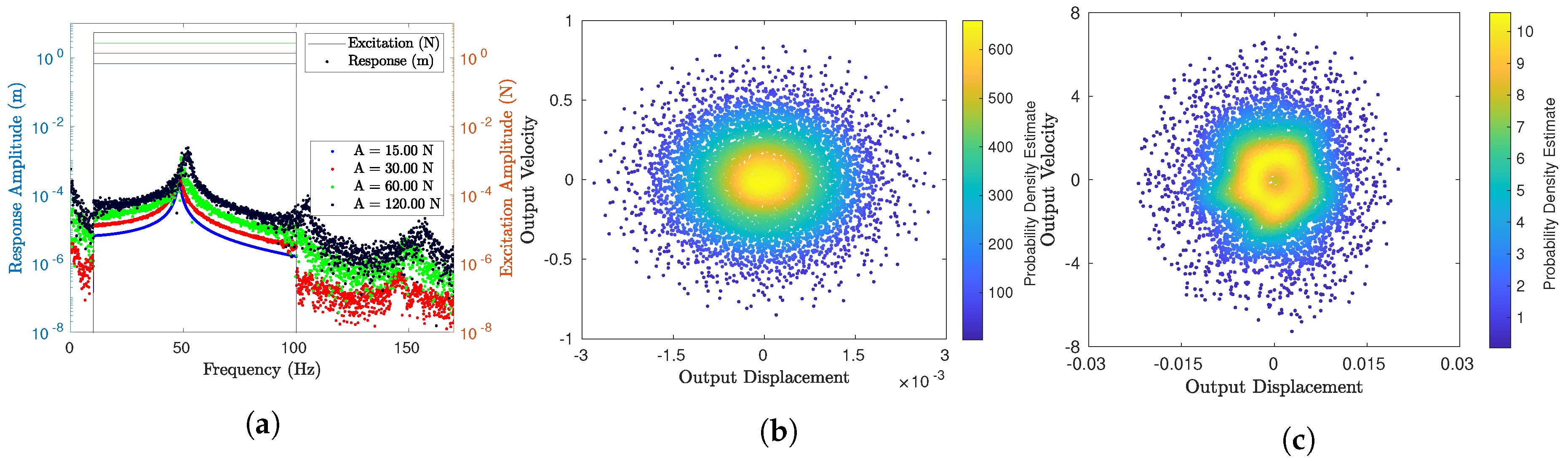
4.3.1. Occurrence of Uncontrolled Higher Harmonics during PLL Testing with Shaker

In Figure 14, the natural frequency and modal damping ratio are depicted as function of the amplitude. For vibrations smaller than the clearance, the unilateral spring is not activated, and the system behaves linearly. Beyond this threshold, the unilateral spring provides additional stiffness.
In contrast to the previous benchmarks, considerable exciter-structure interaction was encountered during PLL testing. As a consequence, the modal properties extracted in the configuration with shaker deviate from those without shaker (Figure 14). In the configuration without shaker, on the other hand, the agreement with the EPMC reference is excellent. This clearly shows that the observed deviations are due to the exciter-structure interaction, rather than due to the imperfect spatial distribution of the forcing (concentrated for PLL testing, distributed for EPMC). The deviation is more pronounced for the modal damping ratio. In fact, the asymptotic limit for large vibrations is different in this case.
To further analyze in what way the exciter-structure interaction leads to inaccurately identified modal properties, the resulting excitation force is illustrated for different vibration levels. Recall that the excitation force is applied as a concentrated load in the case of PLL testing, while it is applied as a distributed load 2 D ω M ̲ ̲ q ̲ ˙ in the case of the EPMC. For the ease of illustration, the resulting scalar modal force is determined with respect to the lowest-frequency linear normal mode ( k n attached), and plotted versus the modal coordinate of the same mode. The results are depicted in Figure 15 and Figure 16 for the case without and with shaker, respectively.
In the case without shaker, the excitation force during PLL testing is harmonic by design. Apparently, the modal displacement is dominated by the fundamental harmonic. Consequently, the force-displacement curve forms an ellipse in the case of PLL testing without shaker (Figure 15). In the case of the EPMC, the self-excitation term 2 D ω M ̲ ̲ q ̲ ˙ also contains higher harmonics in the nonlinear regime. Thus, the force-displacement curve slightly deviates from an ellipse in this case.
In the case with shaker, the excitation force during PLL testing is the result of the harmonic input to the shaker and the exciter-structure interaction. Apparently, the latter leads to strong higher harmonics in the nonlinear regime (Figure 16). Recall that the current implementation of the nonlinear modal testing controls only the fundamental harmonic, while the higher harmonics are uncontrolled. A multi-harmonic control scheme might improve the nonlinear mode isolation, and thus the extracted modal properties, but this was considered beyond the scope of this study.

4.3.2. Identification of the PNLSS Models

For this benchmark, a state-space dimension of two was found to be sufficient. As can be seen from Figure 14, the considered natural frequency is in the range of 48–55 Hz. The multisine signals for the training are designed to have an active frequency band of 10–100 Hz, with a frequency resolution of 0.09 Hz and sampled at a frequency of 4096 Hz for eight periods.
The excitation and response frequency spectra, as well as the spread of the response for two excitation levels are shown in Figure 17, in the format as in the previous sections. The response spectrum reflects the hardening behavior seen also in Figure 14. As in the case of the previous benchmarks, the exciter-structure interaction had an effect on the training data (resonant force drop), but no significant effect on the performance of the PNLSS models.

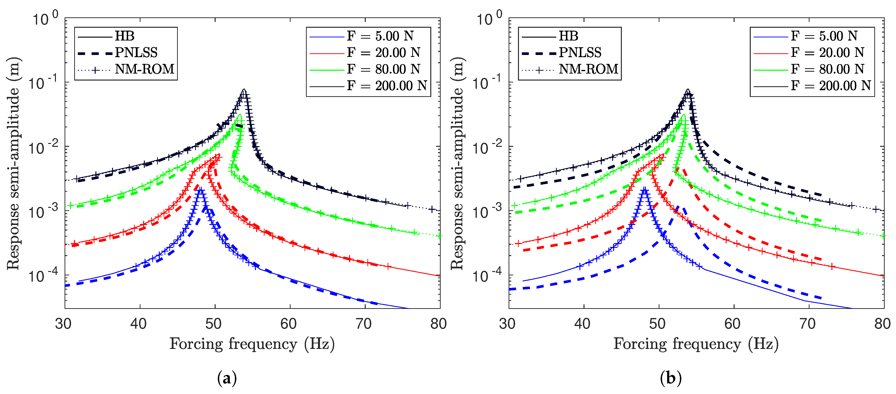
4.3.3. Assessment of the Prediction Accuracy

The quality of the identified NM-ROM and PNLSS models is assessed as for the previous benchmarks. The results are depicted in Figure 18 and Figure 19 for the case of identification without and with exciter-structure interaction, respectively.
The NM-ROM provides excellent accuracy for all levels of the harmonic forcing. One has to carefully compare Figure 18 and Figure 19 in order to see that the NM-ROM identified from PLL testing with shaker slightly underestimates the resonant response at higher levels. This is in full accordance with the overestimation of the modal damping ratio here (Figure 14).
Concerning the performance of the PNLSS models, the statements made for the benchmark with elastic dry friction element apply. In particular, if the PNLSS model is trained at low excitation level, and thus the unilateral spring element is not sufficiently activated, the linearized behavior is extrapolated to high response levels. On the other hand, if the PNLSS model is trained in the nonlinear response regime, remarkable accuracy can be achieved in the corresponding regime, given that third-order polynomials can only coarsely approximate the piecewise linear force-displacement characteristic of a unilateral spring.

5. Conclusions and Outlook

Two nonlinear system identification methodologies were assessed in this paper, the identification of a nonlinear-mode model from feedback-controlled phase-resonant excitation and the identification of a polynomial nonlinear state-space (PNLSS) model mainly from uncontrolled broadband multisine excitation. These were applied to three different benchmarks in order to assess their performance and to inform future improvements of the methodologies. The benchmarks are a geometrically nonlinear clamped-clamped beam (Duffing oscillator), a cantilevered beam with an elastic dry friction attachment, and a cantilevered beam with a unilateral contact attachment.
By design, the two methodologies have a completely different range of utility. A nonlinear-mode model is only applicable to situations where the single-nonlinear-mode theory is valid. In particular, this is the case for mechanical systems driven near primary external resonances, by self-excitation, and combinations thereof. The dynamic regime of interest must be periodic, potentially with slowly varying parameters. As a consequence of these limitations, the secondary resonance peak associated with nonlinear modal interactions, encountered for one benchmark, was missed by the corresponding nonlinear-mode model. In the future, an extension of the range of utility of nonlinear-mode models, for instance to coupled structures, or structures with non-mechanical components would be interesting. In contrast, PNLSS models can describe quite generic dynamic behavior and are not limited to mechanical systems. This large range of applicability comes with a limited range of validity. Although PNLSS models are sometimes viewed as natural representation of multiple-input-multiple-output systems, the current state of the art shows clear limitations. Due to the quick increase of the number of unknown coefficients with the polynomial order, it is common practice to consider polynomial terms of only up to order three. These basis functions cannot be expected to provide an accurate global representation of generic nonlinearities. The inevitable model error induces a dependence of the identified model on the training data. When the PNLSS model was trained at a certain response level, the prediction accuracy near this response regime was remarkably high, even for the non-smooth contact nonlinearities studied in this paper. However, further away from this response level, the accuracy was low, or the response even diverged. In contrast, nonlinear-mode models are highly accurate for generic nonlinearities and any response level (as long as this response level falls within the range specified in the modal analysis).
The two system identification methodologies differ in terms of testing and postprocessing effort. In contrast to the identification of a PLNSS model, the nonlinear modal testing relies on a feedback-controller. In the future, it would be desirable to have a systematic way of tuning the control parameters to ensure a quick and robust testing. While the extraction of the modal properties from the test data is straight-forward, the identification of the PNLSS model’s coefficient matrices requires an involved optimization process. In the future, it would be desirable to make this optimization less sensitive to the initial guess and more computationally efficient.
Some further challenges were found for both methodologies. One of the benchmarks showed that the quality of the extracted modal properties was (slightly) deteriorated by uncontrolled higher harmonics in the excitation force associated with exciter-structure interaction. In the future, it would be desirable to extend the control scheme to higher harmonics. Finally, the PNLSS identification struggles if the training data contains a chaotic response, since then the sensitive dependence on initial conditions and model parameters render the optimization problem ill-posed.

Author Contributions

Conceptualization, M.K., J.-P.N., P.T., and M.R.W.B.; methodology, M.K. and J.-P.N.; software, M.K., J.-P.N., and M.R.W.B.; validation, N.N.B., S.L. and M.S.; formal analysis, N.N.B. and S.L.; investigation, N.N.B. and S.L.; resources, M.R.W.B. and M.K.; data curation, M.S., M.K., J.-P.N., P.T. and M.R.W.B.; writing—original draft preparation, N.N.B., S.L. and M.K.; writing—review and editing, N.N.B., S.L., M.S., M.R.W.B., P.T., J.-P.N. and M.K.; visualization, N.N.B. and S.L.; supervision, M.S., M.K., J.-P.N., P.T., and M.R.W.B.; project administration, M.K., J.-P.N., P.T., and M.R.W.B.; funding acquisition, M.R.W.B. and M.K. All authors have read and agreed to the published version of the manuscript.

Funding

The work was funded by the Deutsche Forschungsgemeinschaft (DFG, German Research Foundation)—Project 402813361.

Acknowledgments

The authors gratefully acknowledge the Tribomechadynamics Research Camp (TRC) 2019, a summer research camp for graduate students held at Rice University in June–July 2019 where much of the research work for this paper was conducted. See http://tmd.rice.edu/tribomechadynamics-research-camp/ for more details.

Conflicts of Interest

The authors declare no conflict of interest.

Abbreviations

The following abbreviations are used in this manuscript:
NM-ROMNonlinear Modal-Reduced Order Model
PNLSSPolynomial Non-Linear State-Space
PLLPhase-Locked Loop
EPMCExtended Periodic Motion Concept

References

  1. Dou, S.; Jensen, J.S. Optimization of nonlinear structural resonance using the incremental harmonic balance method. J. Sound Vib. 2015, 334, 239–254. [Google Scholar] [CrossRef] [Green Version]
  2. Krack, M.; Salles, L.; Thouverez, F. Vibration prediction of bladed disks coupled by friction joints. Arch. Comput. Methods Eng. 2017, 24, 589–636. [Google Scholar] [CrossRef] [Green Version]
  3. Schoukens, J.; Ljung, L. Nonlinear system identification: A user-oriented road map. IEEE Control Syst. Mag. 2019, 39, 28–99. [Google Scholar]
  4. Noël, J.P.; Kerschen, G. Nonlinear system identification in structural dynamics: 10 more years of progress. Mech. Syst. Signal Proces. 2017, 83, 2–35. [Google Scholar] [CrossRef]
  5. Roache, P.J. Verification and Validation in Computational Science and Engineering; Hermosa: Albuquerque, NM, USA, 1998; Volume 895. [Google Scholar]
  6. Alijani, F.; Amabili, M. Non-Linear Vibrations of Shells: A Literature Review from 2003 to 2013. Int. J. Non-Linear Mech. 2014, 58, 233–257. [Google Scholar] [CrossRef] [Green Version]
  7. Brake, M.R.W. The Mechanics of Jointed Structures; Springer Science+Business Media: New York, NY, USA, 2017. [Google Scholar]
  8. Kerschen, G.; Worden, K.; Vakakis, A.F.; Golinval, J.C. Past, present and future of nonlinear system identification in structural dynamics. Mech. Syst. Signal Process. 2006, 20, 505–592. [Google Scholar] [CrossRef] [Green Version]
  9. Scheel, M.; Kleyman, G.; Tatar, A.; Brake, M.R.W.; Peter, S.; Noël, J.P.; Allen, M.S.; Krack, M. System Identification of Jointed Structures: Nonlinear Modal Testing Vs. State-Space Model Identification. In Nonlinear Dynamics; Kerschen, G., Ed.; Springer International Publishing: Cham, Switzerland, 2019; Volume 1, pp. 159–161. [Google Scholar]
  10. Scheel, M.; Kleyman, G.; Tatar, A.; Brake, M.R.W.; Peter, S.; Noël, J.P.; Allen, M.S.; Krack, M. Experimental assessment of polynomial nonlinear state-space and nonlinear-mode models for near-resonant vibrations. Mech. Syst. Signal Process. 2020, 143, 106796. [Google Scholar] [CrossRef]
  11. Rosenberg, R.M. Normal Modes of Nonlinear Dual-Mode Systems. J. Appl. Mech. 1960, 27, 263–268. [Google Scholar] [CrossRef]
  12. Kerschen, G.; Peeters, M.; Golinval, J.C.; Vakakis, A.F. Nonlinear Normal Modes, Part I: A useful framework for the structural dynamicist: Special Issue: Non-linear Structural Dynamics. Mech. Syst. Signal Proces. 2009, 23, 170–194. [Google Scholar] [CrossRef] [Green Version]
  13. Szemplinska-Stupnicka, W. The modified single mode method in the investigations of the resonant vibrations of non-linear systems. J. Sound Vib. 1979, 63, 475–489. [Google Scholar] [CrossRef]
  14. Krack, M.; Panning-von Scheidt, L.; Wallaschek, J. A method for nonlinear modal analysis and synthesis: Application to harmonically forced and self-excited mechanical systems. J. Sound Vib. 2013, 332, 6798–6814. [Google Scholar] [CrossRef]
  15. Jahn, M.; Stender, M.; Tatzko, S.; Hoffmann, N.; Grolet, A.; Wallaschek, J. The extended periodic motion concept for fast limit cycle detection of self-excited systems. Comput. Struct. 2020, 227, 106139. [Google Scholar] [CrossRef]
  16. Heinze, T.; Panning-von Scheidt, L.; Wallaschek, J. Global detection of detached periodic solution branches of friction-damped mechanical systems. Nonlinear Dyn. 2019. [Google Scholar] [CrossRef]
  17. Shaw, S.W.; Pierre, C. Non-Linear Normal Modes and Invariant Manifolds. J. Sound Vib. 1991, 150, 170–173. [Google Scholar] [CrossRef] [Green Version]
  18. Shaw, S.W.; Pierre, C. Normal Modes for Non-Linear Vibratory Systems. J. Sound Vib. 1993, 164, 85–124. [Google Scholar] [CrossRef] [Green Version]
  19. Haller, G.; Ponsioen, S. Nonlinear normal modes and spectral submanifolds: Existence, uniqueness and use in model reduction. Nonlinear Dyn. 2016, 86, 1493–1534. [Google Scholar] [CrossRef] [Green Version]
  20. Krack, M. Nonlinear modal analysis of nonconservative systems: Extension of the periodic motion concept. Comput. Struct. 2015, 154, 59–71. [Google Scholar] [CrossRef]
  21. Jahn, M.; Tatzko, S.; Panning-von Scheidt, L.; Wallaschek, J. Comparison of different harmonic balance based methodologies for computation of nonlinear modes of non-conservative mechanical systems. Mech. Syst. Signal Proces. 2019, 127, 159–171. [Google Scholar] [CrossRef]
  22. Scheel, M.; Peter, S.; Leine, R.I.; Krack, M. A phase resonance approach for modal testing of structures with nonlinear dissipation. J. Sound Vib. 2018, 435, 56–73. [Google Scholar] [CrossRef]
  23. Karaağaçlı, T.; Özgüven, H.N. Experimental modal analysis of nonlinear systems by using response-controlled stepped-sine testing. Mech. Syst. Signal Proces. 2020, 146, 107023. [Google Scholar] [CrossRef]
  24. Renson, L.; Barton, D.A.W.; Neild, S.S. Experimental Analysis of a Softening-Hardening Nonlinear Oscillator Using Control-Based Continuation. In Nonlinear Dynamics, Volume 1: Proceedings of the 34th IMAC, A Conference and Exposition on Structural Dynamics 2016; Kerschen, G., Ed.; Springer International Publishing: Cham, Switzerland, 2016; pp. 19–27. [Google Scholar] [CrossRef]
  25. Renson, L.; Barton, D.A.W.; Neild, S.A. Experimental Tracking of Limit-Point Bifurcations and Backbone Curves Using Control-Based Continuation. Int. J. Bifurc. Chaos 2017, 27, 1730002. [Google Scholar] [CrossRef] [Green Version]
  26. Paduart, J.; Lauwers, L.; Swevers, J.; Smolders, K.; Schoukens, J.; Pintelon, R. Identification of nonlinear systems using Polynomial Nonlinear State Space models. Automatica 2010, 46, 647–656. [Google Scholar] [CrossRef]
  27. Pintelon, R.; Schoukens, J. System Identification: A Frequency Domain Approach; John Wiley & Sons: Piscataway, NJ, USA, 2012. [Google Scholar]
  28. Tiels, K. A polynomial nonlinear state-space toolbox for Matlab. In Proceedings of the 21st IMEKO TC4 International Symposium on Understanding the World through Electrical and Electronic Measurement, and 19th International Workshop on ADC Modelling and Testing, Budapest, Hungary, 7–9 September 2016; pp. 28–31. [Google Scholar]
  29. Schoukens, J.; Pintelon, R.; Rolain, Y.; Dobrowiecki, T. Frequency response function measurements in the presence of nonlinear distortions. Automatica 2001, 37, 939–946. [Google Scholar] [CrossRef]
  30. Morlock, F. Force Control of an Electrodynamic Shaker for Experimental Testing of Nonlinear Mechanical Structures. Master’s Thesis, Universität Stuttgart, Stuttgart, Germany, 2015. [Google Scholar]
  31. Dormand, J.R.; Prince, P.J. A family of embedded Runge-Kutta formulae. J. Comput. Appl. Math. 1980, 6, 19–26. [Google Scholar] [CrossRef] [Green Version]
  32. Krack, M.; Gross, J. Harmonic Balance for Nonlinear Vibration Problems; Mathematical Engineering; Springer International Publishing: Cham, Switzerland, 2019. [Google Scholar]
  33. Nayfeh, A.; Mook, D. Nonlinear Oscillations; Wiley Classics Library, John Wiley & Sons, Ltd.: Hoboken, NJ, USA, 2008. [Google Scholar]
  34. Wolf, A.; Swift, J.B.; Swinney, H.L.; Vastano, J.A. Determining Lyapunov exponents from a time series. Phys. D Nonlinear Phenom. 1985, 16, 285–317. [Google Scholar] [CrossRef] [Green Version]
  35. Krack, M.; Panning-von Scheidt, L.; Wallaschek, J. On the computation of the slow dynamics of nonlinear modes of mechanical systems. Mech. Syst. Signal Proces. 2014, 42, 71–87. [Google Scholar] [CrossRef]
  36. Gaul, L.; Nitsche, R. The Role of Friction in Mechanical Joints. Appl. Mech. Rev. 2001, 54, 93. [Google Scholar] [CrossRef]
  37. Mathis, A.T.; Balaji, N.N.; Kuether, R.J.; Brink, A.R.; Brake, M.R.W.; Quinn, D.D. A Review of Damping Models for Structures With Mechanical Joints. Appl. Mech. Rev. 2020, 72. [Google Scholar] [CrossRef]
  38. Noël, J.P.; Esfahani, A.F.; Kerschen, G.; Schoukens, J. A nonlinear state-space approach to hysteresis identification. Mech. Syst. Signal Proces. 2017, 84, 171–184. [Google Scholar] [CrossRef] [Green Version]
  39. Hurty, W.C. Dynamic analysis of structural systems using component modes. AIAA J. 1965, 3, 678–685. [Google Scholar] [CrossRef]
  40. Craig, R.R.J.; Bampton, M.C.C. Coupling of substructures using component mode synthesis. AIAA J. 1968, 6, 1313–1319. [Google Scholar] [CrossRef]
Figure 1. Diagrams of (a) the geometrically nonlinear clamped-clamped beam model, (b) the Euler-Bernoulli beam model with unilateral contact, (c) the Euler-Bernoulli beam model with elastic dry-friction contact, and (d) the shaker model [22].
Vibration 03 00022 g001
Figure 2. Methodology used for comparing the two system identification approaches.
Vibration 03 00022 g002
Figure 3. Effect of excitation imperfections on the identified modal properties: (a) natural frequency and (b) damping ratio as function of the amplitude.
Vibration 03 00022 g003
Figure 4. (a) The frequency spectrum of the multisine force input and system output for the Duffing oscillator at different input levels; state-space response and its probability density estimate (PDE) under multisine imposed forcing at (b) 0.01 N and (c) 0.5 N root-mean-square (RMS).
Vibration 03 00022 g004
Figure 5. (a) The frequency spectrum of the multisine voltage input to the shaker and system output for the Duffing oscillator at different input levels; state-space response and its probability density estimate (PDE) under multisine imposed voltage at (b) 1.14 V and (c) 57.03 V RMS.
Vibration 03 00022 g005
Figure 6. Response of the Duffing oscillator to multisine input and errors of the best linear approximation (BLA) and the identified polynomial nonlinear state-space (PNLSS) model: (a) A = 0.50 N, (b) A = 0.75 N. Enlarged views from (a,b) are provided in (c,d), respectively.
Vibration 03 00022 g006
Figure 7. Near-resonant frequency responses obtained directly from the benchmark (Duffing oscillator without shaker), the Nonlinear Modal-Reduced Order Model (NM-ROM) and the PNLSS model trained at excitation level (a) 0.01 N, (b) 0.50 N, (c) 0.75 N (without shaker).
Vibration 03 00022 g007
Figure 8. Near-resonant frequency responses obtained directly from the benchmark (Duffing oscillator without shaker), the NM-ROM and the PNLSS model trained at excitation level (a) 1.14 V, (b) 57.03 V, (c) 85.54 V (with shaker).
Vibration 03 00022 g008
Figure 9. Effect of excitation imperfections on the identified modal properties: (a) natural frequency and (b) damping ratio as function of the amplitude.
Vibration 03 00022 g009
Figure 10. (a) The frequency spectrum of the multisine force input and system output for the friction-damped beam at different input levels; and state-space response and its probability density estimate (PDE) under multisine imposed forcing at (b) 0.1 N and (c) 0.8 N RMS.
Vibration 03 00022 g010
Figure 11. Near-resonant frequency responses obtained directly from the benchmark (friction-damped beam without shaker), the NM-ROM and the PNLSS model trained at excitation level (a) 0.01 N, (b) 0.10 N, (c) 0.80 N (without shaker).
Vibration 03 00022 g011
Figure 12. PNLSS training on phase-locked loop (PLL) data: Each subfigure indicates the PLL response time history (black solid lines), time history of the initial PNLSS model (red dashed lines), and the time history of the converged PNLSS model (blue dashed lines). Depicted are the cases for initial PNLSS models trained with multisine data at levels (a) A = 0.10 N and (b) A = 0.80 N. Enlarged views of the rectangular regions in (a,b) are provided in (c,d).
Vibration 03 00022 g012
Figure 13. Near-resonant frequency responses obtained directly from the benchmark (friction-damped beam without shaker), the NM-ROM and the PNLSS model trained with PLL data using as initial guess the PNLSS model trained with multisine data at levels (a) 0.1 N, (b) 0.8 N (without shaker).
Vibration 03 00022 g013
Figure 14. Effect of excitation imperfections on the identified modal properties: (a) natural frequency and (b) damping ratio as function of the amplitude.
Vibration 03 00022 g014
Figure 15. Excitation force during nonlinear modal analysis at four different vibration levels; modal force plotted versus modal displacement with respect to the lowest-frequency linear normal mode; PLL results without shaker in blue; Extended PeriodicMotion Concept (EPMC) results in red.
Vibration 03 00022 g015
Figure 16. Excitation force during nonlinear modal analysis at four different vibration levels; modal force plotted versus modal displacement with respect to the lowest-frequency linear normal mode; PLL results with shaker in blue; EPMC results in red.
Vibration 03 00022 g016
Figure 17. (a) The frequency spectrum of the multisine force input and system output for the beam with unilateral spring at different input levels; and state-space response and its probability density estimate (PDE) under multisine imposed forcing at (b) 15 N and (c) 120 N RMS.
Vibration 03 00022 g017
Figure 18. Near-resonant frequency responses obtained directly from the benchmark (beam with unilateral spring without shaker), the NM-ROM and the PNLSS model trained at excitation level (a) 15 N, (b) 120 N (without shaker).
Vibration 03 00022 g018
Figure 19. Near-resonant frequency responses obtained directly from the benchmark (beam with unilateral spring without shaker), the NM-ROM and the PNLSS model trained at excitation level (a) 750 V, (b) 6000 V (with shaker).
Vibration 03 00022 g019
Table 1. Parameters of the shaker model (refer to Figure 1d for contexts) used for all simulations.
DescriptionParameterValue
Electrical resistanceR3 Ω
Electrical inductivityL140 mH
Shaker force generating constantG15.4791 NA 1
Coil mass m C 0.019 kg
Coil stiffness k C 8.4222 × 10 7 Nm 1
Coil damping d C 57.1692 Nsm 1
Table mass m T 0.0243 kg
Table stiffness k T 20707 Nm 1
Table damping d T 28.3258 Nsm 1
Stinger stiffness (idealized as a bar) k S t i n g e r A s t i n g e r E s t i n g e r / s t i n g e r
( 4 π mm 2 ) × ( 210,000 N mm 2 ) / ( 0.02 m )
Table 2. Leading Lyapunov exponents estimated from the time series of the response of the Duffing oscillator to multisine excitation.
Input LevelLyapunov Exponents (bits/s)
A (N) λ 1 λ 2
0.01−26.7−28.0
0.25−22.9−31.8
0.50−7.9−46.9
0.755.7−60.4

