Simplified Analysis for Multiple Input Systems: A Toolbox Study Illustrated on F-16 Measurements

Abstract

This paper introduces a nonparametric, nonlinear system identification toolbox called SAMI (simplified analysis for multiple input systems) developed for industrial measurements of vibro-acoustic systems with multiple inputs. It addresses the questions related to the user-friendly (semi-)automatic processing of multiple-input, multiple-output measurements with respect to the design of an experiment and the analysis of the measured data. When the proposed toolbox is used, with minimal user interaction, it is easily possible (a) to decide whether the underlying system is linear or not, (b) to decide whether the linear framework is still adequate to be used, and (c) to tell an inexperienced user how much can be gained using an advanced nonlinear framework. The toolbox is illustrated on openly accessible F-16 ground vibration testing measurements.

1. Introduction

The goal of this paper is to introduce a simple but efficient nonlinear, nonparametric toolbox for the automated analysis of vibro-acoustic industrial measurements. The goal of vibration testing is to obtain experimental data for a whole vibrating structure such as a road or air vehicle. Using these data, it is possible to validate and improve the dynamic models of systems under test. Since the development of advanced digital signal processing, it became possible to use a large variety of user-defined excitation signals to experimentally determine the broadband frequency response functions (FRFs), which are required to obtain parametric models (e.g., resonance frequencies, modes shapes). In this paper, special multisines (also known as pseudo-random noise signals) are considered excitation signals. The main advantage of the proposed signals is that there is no problem with spectral leakage or transience, and they deliver excellent linear models while providing useful information about the measurement.

Many vibro-acoustic structures are inherently nonlinear. As coping with nonlinear systems became increasingly important, numerous modeling methods were proposed. For a general overview of the nonlinear modeling techniques, we refer to [1,2,3,4]. For complexity reasons, nonlinear systems are often approximated with linear systems, because that theory is well-understood, and the cost of nonlinear modelling can be very high. However, the loss of accuracy by this decision is rarely studied. To this end, using the proposed toolbox, it is easy to tell how much can be gained by using an advanced nonlinear modeling technique in order to make a well-balanced decision.

The state-of-the-art modeling tool known as the best linear approximation (BLA) framework is already available for single-input, single-output (SISO) systems [5,6,7,8,9]. Unlike in the SISO case, the design and analysis of a multiple-input, multiple-output (MIMO) experiment are more involved, and the complexity grows with the number of input and output channels. Further, to properly analyze the estimation results and to troubleshoot, an experienced user is needed. This work extends the BLA methodology to MIMO systems with a large number of input and output channels, and it provides an automated, user-friendly interpretation of the measurement data by extracting the user-relevant information, thereby reducing the interactions from the few days needed to evaluate hundreds of transfer functions manually to a couple of minutes. This automatic processing includes, amongst other things, MIMO excitation signal design, transient analysis, estimation method choice, highlighting strategic information (e.g., nonlinearity detection), and warning the system (e.g., indication of sensory faults).

This paper is organized as follows. Section 2 briefly describes the considered systems, assumptions, and BLA framework applied in this work. Section 3 introduces the main components of the toolbox. Section 4 provides an experimental illustration of the ground vibration testing of an F-16 aircraft. Conclusions can be found in Section 5.

2. Basics

2.1. Definitions and Assumptions

The considered systems are electronic, mechanical, or civil dynamic vibrating structures. The dynamics of a linear MIMO system can be nonparametrically characterized in the frequency domain by its frequency response matrix (FRM, a matrix whose elements are FRFs [10]) $G$ at frequency index k, which relates $n_i$ inputs $U$, to $n_o$ outputs $Y$ obtained from data records with a length of N:

$$Y\left[k\right]=G\left[k\right]U\left[k\right]$$

(1)

where $G\left[k\right]\in C^{n_o\times n_i}$, $Y\left[k\right]\in C^{n_o\times 1},U\left[k\right]\in C^{n_i\times 1}$, $k=0\dots \left(N-1\right)/2$ at frequency $f_k=k{f}_s/N$ with sampling frequency of $f_s$. In order to make the text more accessible, the frequency indices and dimensionalities will be omitted.

The system represented by $G$ is nonlinear when the superposition principle is not satisfied in steady state [11]. In this work an arbitrary number of input and output channels is considered. The underlying systems are damped, bounded-input, bounded-output stable, time-invariant, nonlinear systems where the linear response of the system is still present, and the output of the underlying system has the same period as the excitation signal (i.e., the system has PISPO behavior: period in, same period out [11]). The output is measured with additive, independent and identically distributed Gaussian noise (denoted by $E$) with zero mean and finite variance, and it can contain (a smooth, decaying) transient response (denoted by $T$) such that the measurement $Y_{measured}$ is given by:

$$Y_{measured}=Y+E+T=GU+E+T$$

(2)

2.2. Measurement and Instrumentation

The toolbox relies on the use of classical instrumentation and measurement setups [12]. The reference (excitation) signal is an ideal multisine (pseudo-random noise) generated by the toolbox. Multisines are generated in the frequency domain: the magnitudes are freely set by the user, but the phases are randomly chosen [13]. As a result, the signals have a Gaussian distribution. The excitation system (e.g., a shaker) receives the reference signal (e.g., voltage signal) and generates the input signal (e.g., force) to the system (e.g., a vehicle). The output signals (e.g., accelerations) contain the waveforms of the system’s reaction to the input signal. It is important to stress that the toolbox requires the measured time domain signals to be stored.

From an instrumentation point of view, it is assumed that the measurement system is perfectly synchronized, the sampling frequency is kept constant, the input signal is measured precisely such that the signal-to-noise ratio (SNR) is at least 20 dB; otherwise, the FRM estimate will be biased. However, if the reference signal is available, then the toolbox can compensate for the bias by the appropriate choice of estimator [13,14,15].

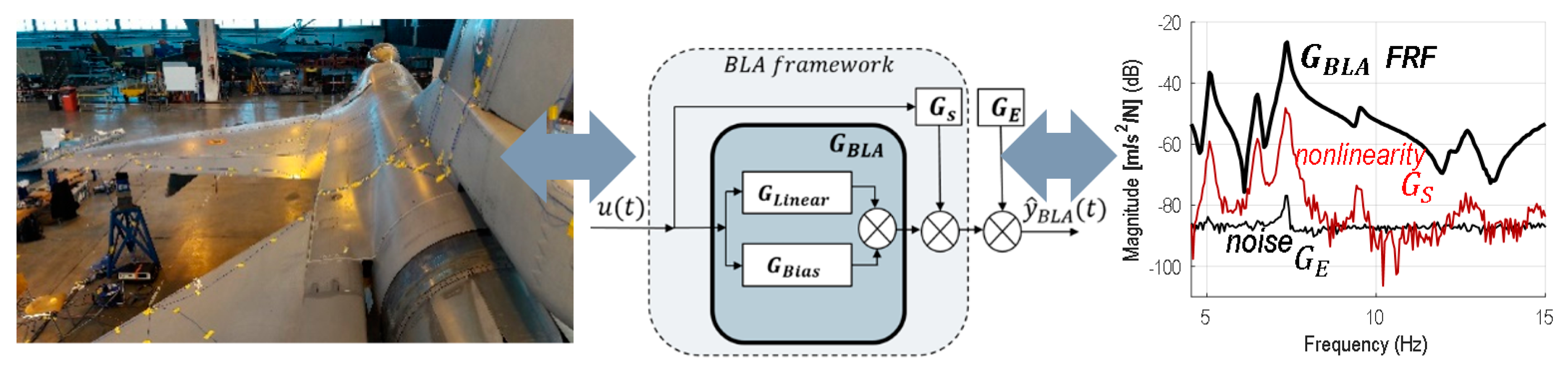
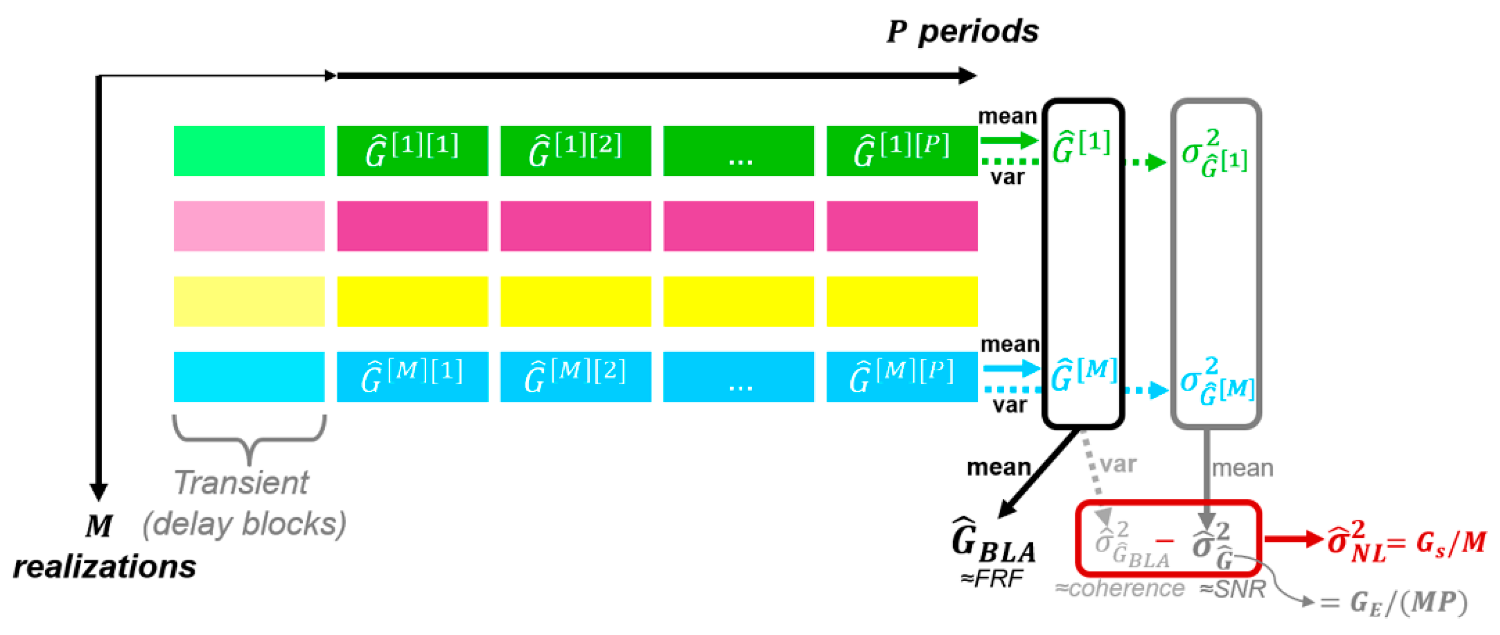
2.3. Best Linear Approximation Framework

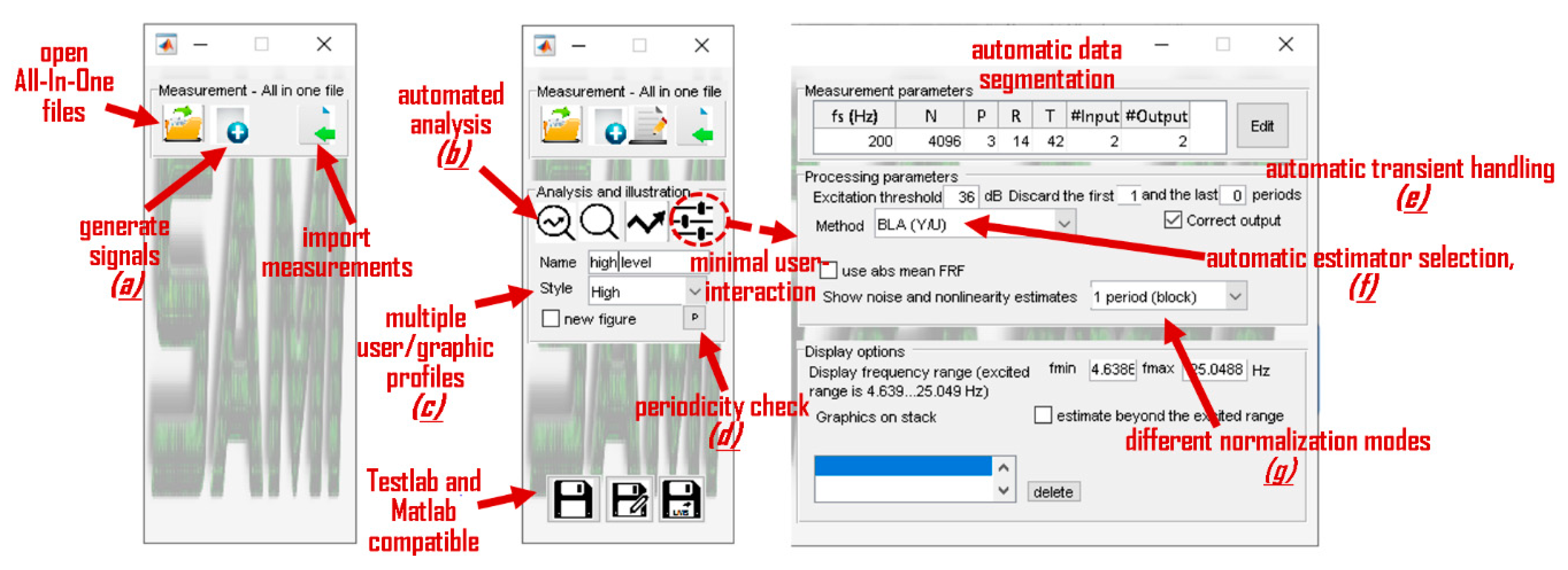
The best linear approximation (BLA) of a nonlinear system is a modelling approach that minimizes the mean square error between the measured output of a nonlinear system and the output of the linear model [13]. It makes use of the knowledge that the excitation signal has both stochastic and deterministic properties. The excitation signal is a random phase multisine signal with M different (random phase) realizations; each of the blocks (periods) is repeated P times. By using multiple realizations (i.e., random phase rotations) of the multisines, the richness of the signal is increased. Instead of directly using the averaged input and output data (i.e., the use of classical H1 framework [12,16]), a partial BLA estimate is calculated for each period of the excitation [11]. A BLA FRM estimate (see Figure 1), for a given signal, is then calculated via the average of partial BLA estimates (see Figure 2). In this case we can easily estimate the noise and nonlinearity levels.

Figure 1 shows the theoretical structure of the considered BLA estimator. In this figure, $G_{linear}$ is the linear (transfer function), phase coherent component of the model for which phase rotations at the input result in a proportional phase rotation at the output [11]. For the cases in which the output has phase non-coherent behavior, we can capture the (non-coherent) nonlinearities represented by $G_s$. Increasing the number of random realizations of the multisine signal allows us to tackle the random output phase rotations as a “half-stochastic” (nonlinear) noise source. The “half-stochastic” term refers to the fact that $G_s$ does not vary over the repetitions of the same signal segment but only over different realizations. $G_E$ represents the classical FRF measurement noise. The usage of periodic excitation reduces the effects of the measurement noise component $G_E$ (see Equation (3)). The usage of multiple realizations reduces the impact of non-coherent nonlinearities represented by $G_s$. $G_{Bias}$ represents the nonlinearities remaining after multiple realizations of the excitation signal.

The considered steady-state model at period $p$ and realization $m$ at excited frequency bins is given as a straightforward extension of Figure 1 by:

$${\widehat{G}}^{\left[m\right]}=\underset{the method for calculation}{\underbrace{\frac{1}{P}{\displaystyle \sum }_{p=1}^P\stackrel{measured FRFs in m}{\overbrace{Y_{measured}^{\left[m\right]\left[p\right]}{U}^{\left[m\right]}{}^{-1}}}}} = \underset{theoretical values}{\underbrace{\frac{1}{P}{\displaystyle \sum }_{p=1}^P(\stackrel{\begin{array}{c}FRF\\ estimate\end{array}}{\overbrace{{\widehat{G}}_{BLA}^{\left[m\right]}} }+\stackrel{\begin{array}{c}nonlinearity\\ fixed in m\end{array}}{\overbrace{{\widehat{G}}_S^{\left[m\right]}}}+\stackrel{\begin{array}{c}noise\\ varies over p\end{array}}{\overbrace{{\widehat{G}}_E^{\left[m\right]\left[p\right]}}})}}$$

(3)

If there is a transient term present in the measurement, it is either discarded or estimated [16]. For computational optimality, the FRM estimation is solved output-channel-wise (i.e., one output channel per unit time). The BLA estimate is calculated at the excited frequency lines only. In the frequency band of excitation, the BLA estimates at the non-excited bins are obtained by (linear) interpolation.

A partial FRM estimate is obtained via averaging over the $P$ periods (blocks) in a realization; see Equation (3). If $P$ is sufficiently large, then (considering the law of large numbers and the distribution properties of the measurement noise) the term ${\widehat{G}}_E^{\left[m\right]}$ in Equation (3) converges to zero. Because the stochastic nonlinear contribution ${\widehat{G}}_S^{\left[m\right]}$ does not vary over the $P$ repetitions of the same realization, one has to average over the $M$ different realizations. If $M$ is sufficiently large, then the nonlinear noise source ${\widehat{G}}_s$ in Equation (3) converges to zero. After the 2D averaging (i.e., averaging over $P$ and $M$) the BLA estimate is obtained. The method is illustrated in Figure 2. The noise covariance ${\widehat{\sigma }}_{\widehat{G}}^2$ is estimated from the improved averaged sample variance ${\widehat{\sigma }}_{{\widehat{G}}^{\left[m\right]}}^2$ of each FRM realization (${\left|X\right|}^{.2}$ represents elementwise squaring and absolute value of the elements of matrix $X$):

$${\widehat{\sigma }}_{\widehat{G}}^2=\frac{1}{M}{{\displaystyle \sum }}_{\mathrm{m}=1}^M\frac{{\sigma }_{{\widehat{G}}^{\left[m\right]}}^2}{M}\mathrm{with}{\widehat{\sigma }}_{{\widehat{G}}^{\left[m\right]}}^2=\frac{1}{P}{{\displaystyle \sum }}_{p=1}^P\frac{{\left|{\widehat{G}}^{\left[m\right]\left[p\right]}-{\widehat{G}}^{\left[m\right]}\right|}^{.2} }{P-1}$$

(4)

where in ${\widehat{\sigma }}_{{\widehat{G}}^{\left[m\right]}}^2$ the additional normalization with $P$ is needed to show the improved covariance (noise) estimate (this term corresponds to $G_E/P$). In other words, averaging over repeated blocks results in an improvement of the SNR. Similarly, the additional normalization with $M$ in ${\widehat{\sigma }}_{\widehat{G}}^2$ is needed to show the noise estimate improvement over different realizations (this term corresponds to $G_E/MP$). If the user wants to see the covariance (noise) with respect to one period (block), one has to multiply ${\widehat{\sigma }}_{\widehat{G}}^2$ with $MP$ (this normalization is used in Figure 1).

The total variance of the FRM ${\widehat{\sigma }}_{{\widehat{G}}_{BLA}}^2$ is estimated from the improved variance (i.e., with extra normalization factor $M$) of each partial BLA estimate ${\widehat{G}}^{\left[m\right]}$:

$${\widehat{\sigma }}_{{\widehat{G}}_{BLA}}^2=\frac{1}{M}{{\displaystyle \sum }}_{m=1}^M\frac{{\left|{\widehat{G}}^{\left[m\right]}-{\widehat{G}}_{BLA}\right|}^{.2}}{M-1}$$

(5)

The difference between the total variance and the noise variance is an estimate of the variance of the stochastic nonlinear contributions such that ${\widehat{\sigma }}_{NL}^2={\widehat{\sigma }}_{{\widehat{G}}_{BLA}}^2-{\widehat{\sigma }}_{\widehat{G}}^2$. If the user wants to see nonlinear contributions with respect to one period (block), he/she has to multiply ${\widehat{\sigma }}_{NL}^2$ with $M$ (this normalization mode is used in Figure 1). For the interpretation of different normalization modes, see Section 4.5.1 and Section 4.5.2. For the detailed calculation, we refer to [11,14].

3. The Toolbox

3.1. Introduction

Simplified analysis for multiple input systems (SAMI) is a user-friendly, Matlab-based toolbox, at its present state available for academic usage per request. It supports command line and graphical user interfaces. The toolbox has been tested with many simulations and real-life industrial measurements, and it is optimized for MIMO experiments. The key idea is to make use of the statistical properties of the proposed excitation signal such that it becomes possible to split up the classical coherence function into noise, nonlinearity (and transient) components.

The toolbox provides a user-friendly interpretation of the nonlinear MIMO measurement data by extracting the user-relevant information and it addresses the questions related to the automatic processing of MIMO measurements with respect to the whole process. The warning-notification system was developed by experiences learned from typical mistakes which popped up during the measurement campaigns. The internal software architecture of SAMI consists of the following interconnected layers:

• The design of experiment layer addresses the signal design, and the choice of measurement parameters.
• The pre-processing layer considers a check-up of the input (reference) channels and provides an early warning to the user when the inputs are too strongly correlated. Furthermore, it segments the measurement data over the periods and realizations, and it sets up the processing parameters for the BLA estimation.
• The BLA estimation layer provides the BLA FRF estimation, calculates advanced statistics of the noise and nonlinearity, and when it applies, estimates the transient term.
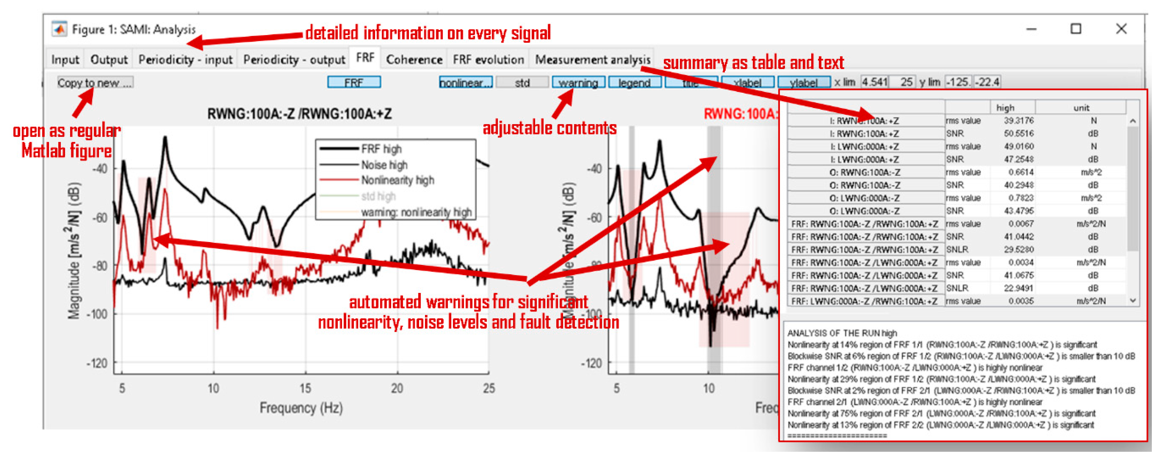
• The post-processing layer makes the estimation results and warnings accessible in a condensed form. It provides users with the FRF, noise, and nonlinearity estimates. It is possible to automatically highlight the FRF (or input, output, reference) channels that have significant nonlinearity or noise levels based on the user-defined profiles. Furthermore, channels with sensory faults and/or imperfections, and correlated inputs are detected as well.

The communication between internal layers is via the all-in-one format of the toolbox: a single structure containing all the measurement, processing and estimation information. Figure 3 shows an overview of the SAMI’s GUI. The displayed content is dynamic; under normal circumstances there is minimal user-interaction required (the details of the measurement and processing parameters are hidden); however, the user can overwrite any of the parameters.

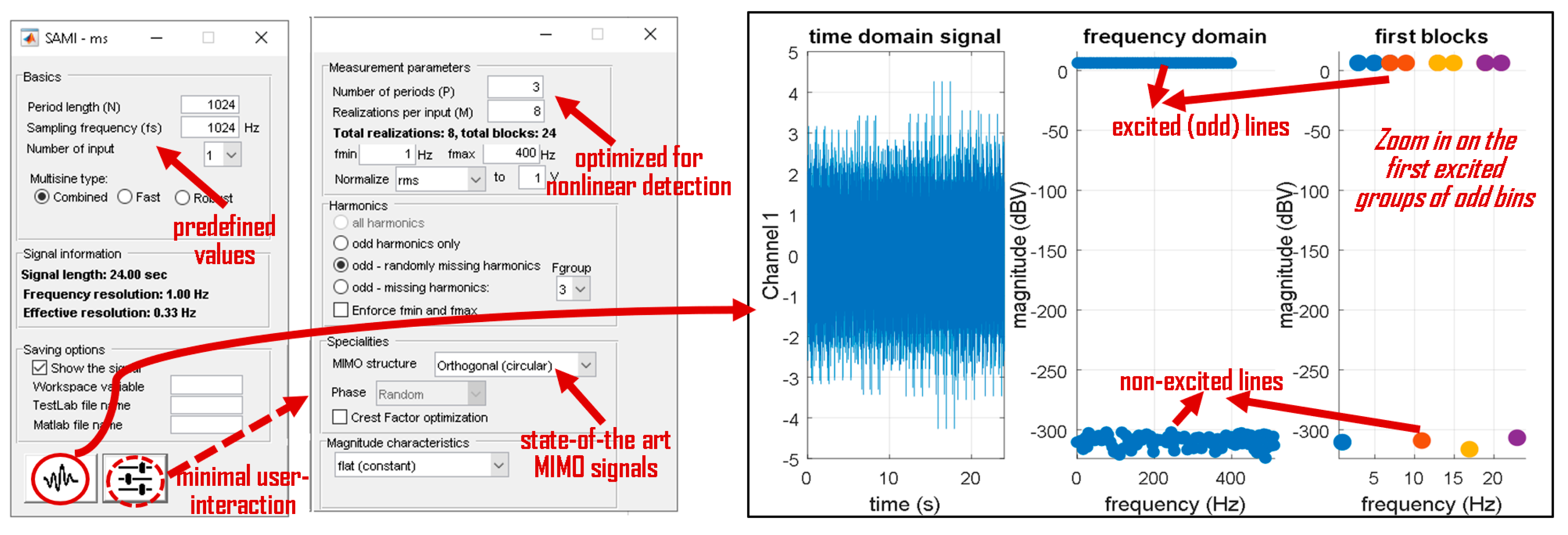
3.2. Multisine Signals

The toolbox uses multisine signals to assess the underlying systems in a time-efficient way [13]. In order to avoid any spectral leakage, to reach full nonparametric characterization of the noise, and to be able to detect nonlinearities, a periodic signal is needed. Many users prefer noise excitations, because they seem easier to implement, but in this case, nonlinearities are not directly identifiable, and there is a possible leakage error. The best signal that satisfies the desired properties is the easy to implement and apply a (random phase) multisine signal which looks like white noise and behaves like it, but it is not noise. If the multisine contains all/only odd or even harmonics, then it is called a full (band)/odd or even multisine. The usage of an odd multisine with randomly missing harmonics allows one to distinguish between even and odd nonlinear distortions on the non-excited bins (called the detection lines).

Basically, there are three modes supported in the toolbox: (1) combined (default, multiple random realizations and periods of missing odd); (2) fast (one realization, multiple periods of missing odd); and (3) robust (multiple realization of full) multisines. For a detailed overview of excitation signals we refer to [10,12]. The multisine module of SAMI with a signal illustration is shown in Figure 4.

3.3. Measurement Processing

Once the measurement is available, it can be easily processed with the toolbox. In most cases, automated data segmentation is used to retrieve the blocks (i.e., the individual periods and realizations). If meta-information is available, then the automated segmentation parameters are compared with the meta-information (or with the manually given information). If there is a significant difference between these, a warning is given. The automated warning system is based on a user-profile and can be changed any time. The toolbox works best with the generated signals; however, other type of excitation signals (noise, sine sweep, etc.) can be processed as well. Once the measurements are processed, a new window appears with the detailed analysis of the measurement. An example for a (MIMO) measurement of the F-16 aircraft is shown in Figure 5. The SISO F16 benchmark data is elaborated on in the next section.

Figure 6 shows another interesting case with which to highlight the capabilities of the toolbox. A lowly damped car structure has been tested using 100 blocks of MIMO multisines; each block is 2 s long, the transient is 6 s (i.e., 3 blocks) long. The figure illustrates the situation which occurs if only one measured block is available: the classical H1 [16], windowed H1 [18,19], and the automated choice (in this case a special implementation of local rational method [15]) are compared with each other.

4. Experimental Illustration

4.1. F16 Measurement

This section concerns the ground vibration testing measurement campaign of a decommissioned F-16 aircraft with two dummy payloads mounted at the wing tips; see Figure 7. The detailed description of the measurement and benchmark data are openly accessible [20].

The right wing is excited by a shaker using combined multisines: odd multisines with skipping one random bin within each group of four successively excited odd lines. This sparse grid is used to detect even and odd nonlinear contributions. The sampling frequency is 400 Hz, and the period length 16,384 samples. The reference (voltage), input (force), and output (accelerations) signals are measured. The range of excitation is between 1 and 60 Hz; there are three periods and nine realizations per excitation level. There are three different input levels measured at 12.2, 49.0, and 97.1 N RMS.

In the 1–15 Hz band, the aircraft possesses about 10 resonance modes. The first few modes below 5 Hz correspond to rigid body motions of the structure. The first flexible mode around 5.2 Hz corresponds to wing bending deformations. The mode involving the most substantial nonlinear distortions is the wing torsion mode located around 7.3 Hz: the mounting interface of the payload features nonlinearities in stiffness and damping, due to clearance and friction. Therefore, the analysis is shown for the 1–15 Hz domain at the payload connection.

4.2. Data Processing

The data processing is fully automated by the toolbox. In short, the first step is the automated segmentation of data: retrieving the periods and realizations. Next, the trends (such as the mean/offset values) from the individual segments are removed [13] and the transient is analyzed. Last, an early quality assessment of experimental data is done, and the parameters for the estimation procedure are set. Based on the SNRs of the input-output data, the existence of a reference signal, the number of periods, and the length of the transient, an appropriate estimator is automatically set.

Currently, the automated possibilities include BLA, H1, indirect BLA [13], and special implementations of the LPM (local polynomial method [10]), LRM (local rational method [15]), indirect LPM, and LRM. Note that with manual overriding more estimation methods are available. This section contains the results of the following single-line Matlab code directly used on the benchmark data: CreateAnalyzePlotAIO(Force(:), Acceleration(2,:),Voltage(:),Fs).

As can be seen, the toolbox requires only the signals in vector/matrix form, and optionally the sampling frequency (if it is not set, then a normalized frequency scale is used). The figures shown in this paper were obtained from the toolbox (for accessibility resized, with no warnings).

Figure 8 shows the visualization of toolbox transient check-up routine. The left side of the figure shows the acceleration (output) measurement at the payload connection. In order to determine the length of the transient (i.e., the number of delay blocks), the last block (period)-assumed to be nearly in steady-state is subtracted from every preceding block. Because the transient decays as an exponential function, the differences are shown in logarithmic scale. Using automated statistical analysis of all available signals, the transient term is estimated as one block. Because there are more than two transient-free periods available, the input-output signals are measured sufficiently good (see next subsection). Because the reference signal is available, the indirect BLA estimator is automatically selected [13].

4.3. Reference and Input Signal

It is crucial to analyze the excitation system and to quantify its accuracy and linearity. For that reason, the reference signals (generated multisine signals) are measured as well. From a system identification point of view, the actuator (shaker) can be seen as a SISO system (with voltage signal as input, the force signal as output). The reference, input signals, and the BLA estimate of the shaker used in this experiment are shown in Figure 9, at the low, medium, and high level of excitation. The left figure shows the generated reference (voltage) signals and their noise estimates. This measurement has very good quality (SNR is greater than 75 dB); the even and odd nonlinear distortions are hidden in the noise.

The excitation forces (see middle figure) are measured with approximately 50–80 dB SNR. It is interesting to point out that the highest input signal is 18 dB higher than the lowest one, but the SNR is decreased with around 8 dB. This indicates the presence of (weak) nonlinearities at the excitation system. Similarly, this information can be seen by looking at the even and odd distortions: the higher the excitation, the higher the nonlinearities with an odd dominance (even distortions usually pop up as noise in the measurement, odd distortions usually influence the shapes of the spectrum).

The BLA analysis of the shakers is shown in the right figure. As can be seen, nonlinear distortions are present which are most likely due to (1) imperfections of the shaker; (2) the interactions between the aircraft and the shaker. Overall, the measurement quality (the gap between the actuator transfer function and its nonlinear estimates) is good, much higher than 20 dB needed to fulfil the assumption on the precise excitation signal measurement.

4.4. Payload Measurement

Further, in order to simplify the analysis, the output and FRF are shown at the payload connection only. The output (acceleration) measurements are shown in Figure 10. As can be seen, the SNR is around 40–50 dB at the resonances. At the higher excitation level, the SNR decreased with approximately 10 dB with respect to the lowest level excitation.

It can also be observed that the resonances were shifted, which is also a further indication of nonlinearities. This is due to the fact that at higher level of excitation we have dominant odd distortions, which usually manifest in changing resonance locations and shapes (it is the so-called hardening or softening stiffness nonlinearity effect).

Please note that even distortions usually manifest as excessive noise on the measurement (see Figure 9).

When the actuator is imperfect, the interpretation of the levels on the detection lines at the output can be jeopardized. If there is power on the (non-excited) detection lines at the input signal power, then the output signals will contain not only the nonlinearities due the system but also the nonlinear contributions of the actuator. However, the toolbox automatically cleans up the output spectrum with the impurities of the actuator [13].

4.5. FRF Analysis

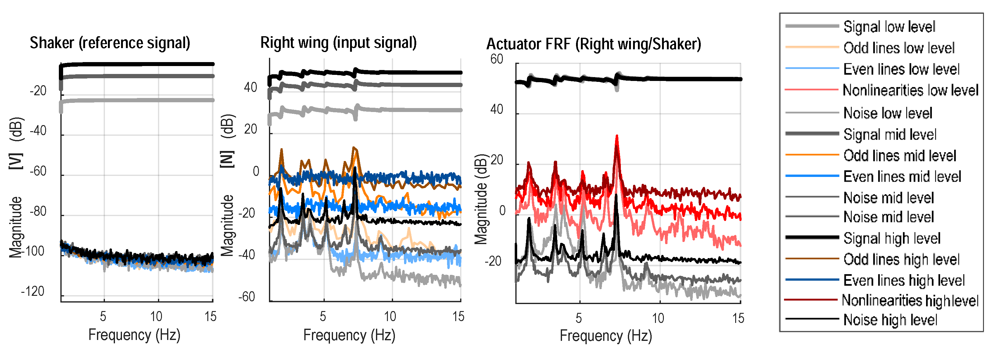
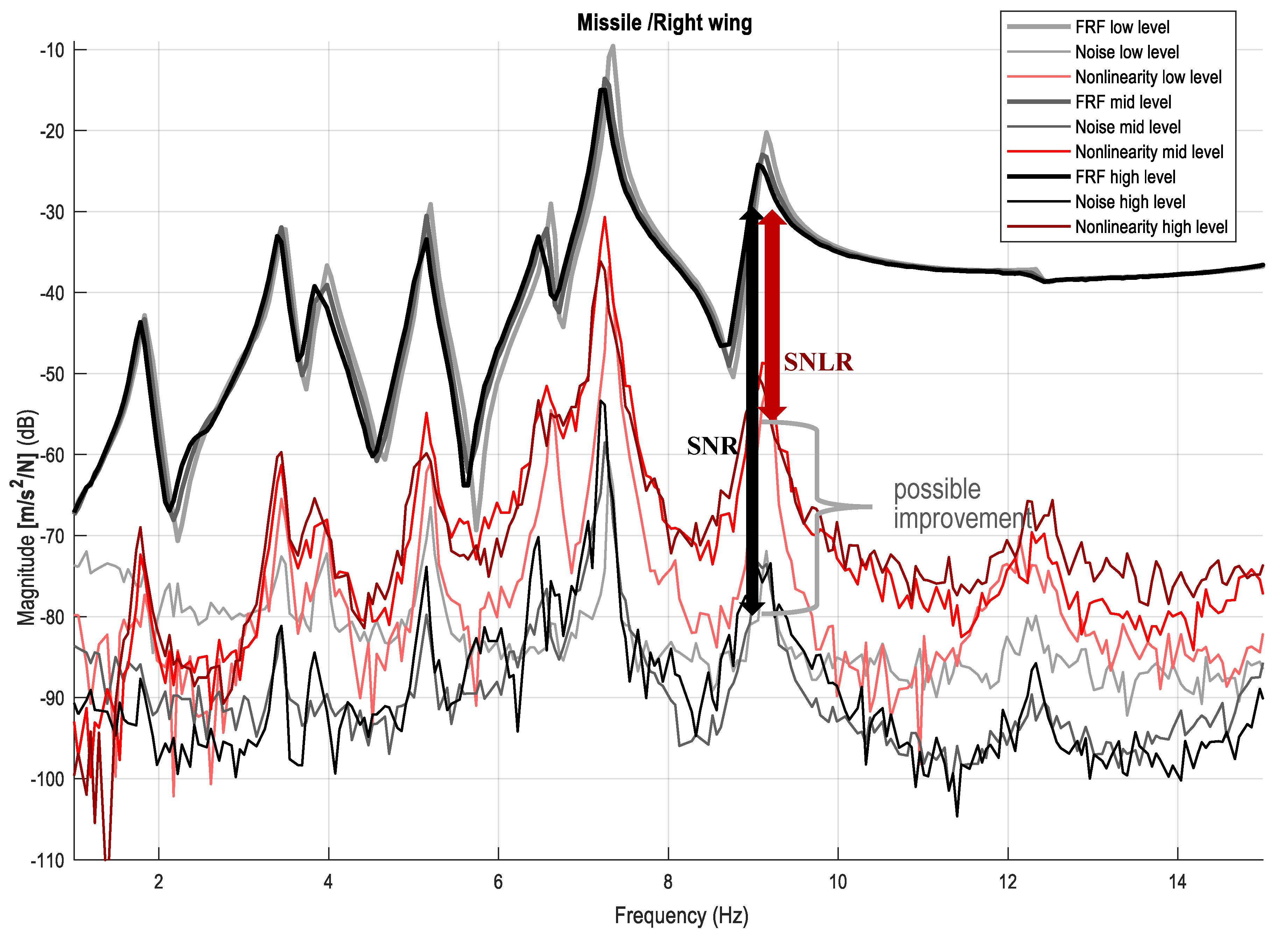
4.5.1. FRFs at Different Excitation Levels

Figure 11 shows the FRFs at low, medium, and high levels of excitation. This is the classical approach; FRFs at multiple levels of excitation are compared with each other. It is interesting to point out that despite the fact that the highest excitation is only 18 dB higher than the lowest level excitation, it can be clearly observed that FRFs at different levels differ a lot from each other by, for instance, shifting resonances and varying damping. This clearly indicates the presence of nonlinearities.

However, for a given level of excitation, an inexperienced user is not able to determine if there are nonlinearities present using the classical approach. The usage of the proposed multisines allows us to obtain noise and nonlinearity level estimations, as explained in Section 2.2. With the help of these curves one can distinguish between the effects of noise and nonlinearity on the coherence. For instance, when looking at the high-level excitation case, the most dominant resonance (around 7.3 Hz) has an approximate SNR of 43 dB, and an SNLR (signal-to-nonlinearity ratio) of 15 dB. This means that at that resonance the main error source is the nonlinearity. If a linear model is used, then the expected error level will be in the order of the SNLR. If an appropriate nonlinear model is used, the expected error level could drop to the SNR. This kind of extra information would have been impossible to derive from the H1 framework.

Furthermore, the toolbox provides an automated warning system for the FRF, actuator, reference, input, and output signals when significant nonlinearities, noise, sensory faults, and correlation issues are discovered. This is partly illustrated in Figure 5.

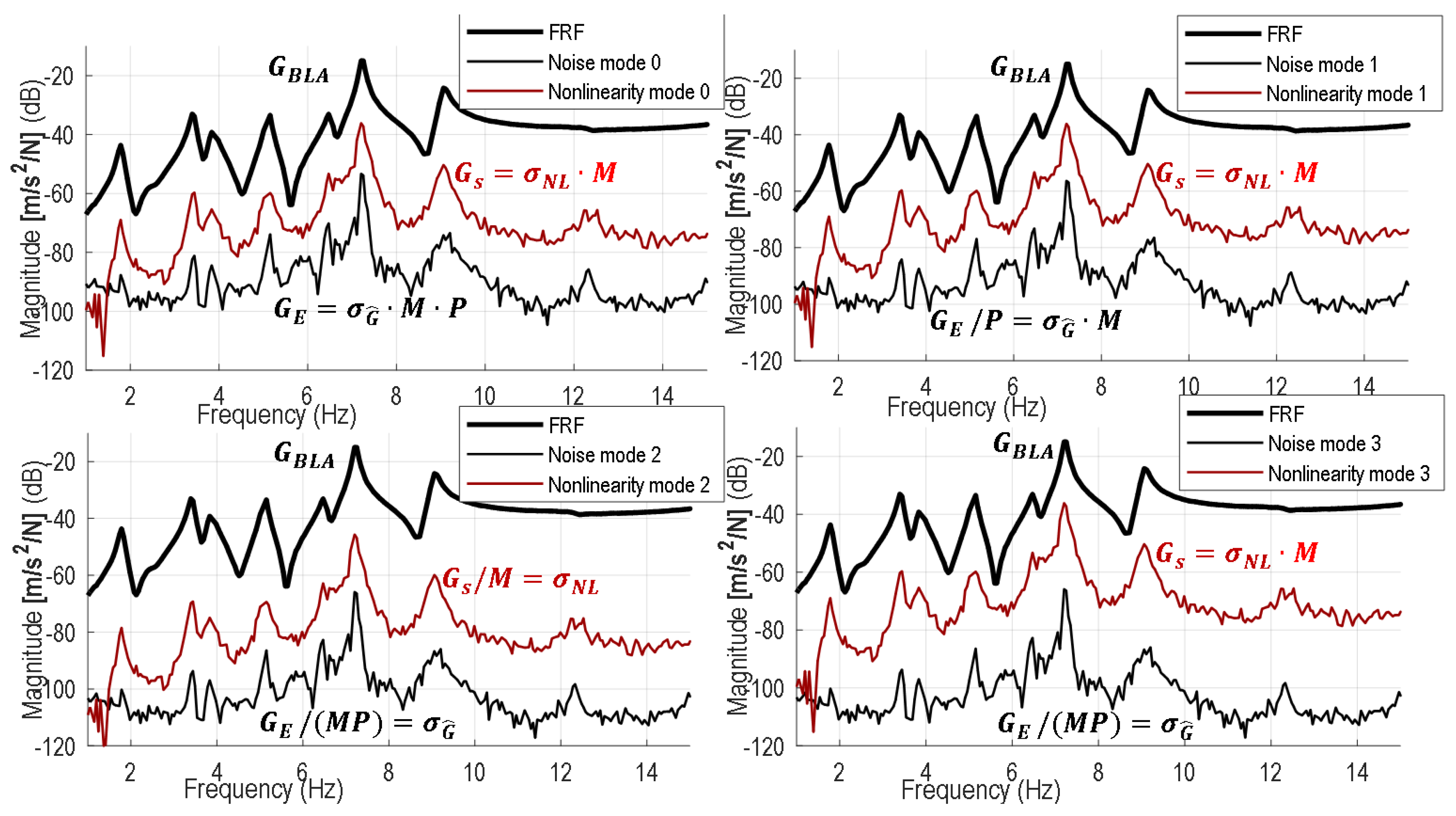
4.5.2. Normalization Modes.

Figure 11 above shows the noise and nonlinearity estimates normalized with respect to one block (period). This normalization mode is very important for understanding, modeling, simulation, and control. Of course, it is possible to show the improved noise and nonlinearity estimates with respect to the whole experiment (measurement). The toolbox supports four different normalization modes illustrated in Figure 12: block-wise (default), realization-wise, and experiment-wise normalization modes, and nonlinear detection mode. We authors recommend always checking the period-wise (block-wise) noise and nonlinearity levels first (mode 0). Using many realizations and simultaneously showing the improved nonlinearity level (experiment-wise normalization, mode 2) might give an incorrect message to the user, since it converges to zero. It is also possible to show the noise improvement over one realization while freezing the nonlinearity level (mode 1). The last normalization mode (nonlinear detection mode, mode 3) can be used to detect the presence of nonlinearities (nonlinear variability mode). The transition between different noise and nonlinear modes can be seen in Figure 2 as well.

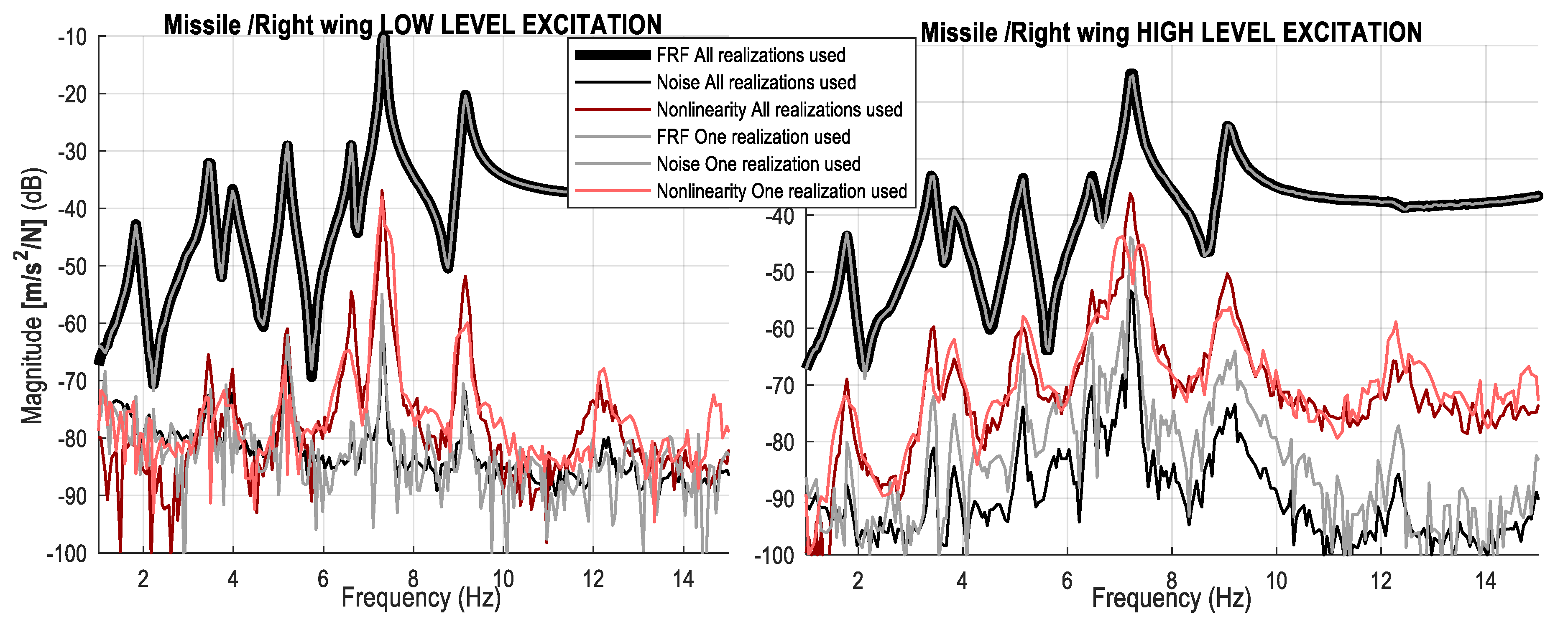
4.5.3. Using One Realization

We authors recommend using as many realizations (and periods) as possible. However, it is sometimes not possible to measure for long. Using the proposed multisines, it is possible to have a rough estimate about the nonlinearity and noise levels using at least one realization and two periods. In the classical literature [13] the one-realization case is called the fast method; the multiple realizations case (with full multisines) is called the robust method, where robust refers to the robustness estimate of the nonlinear and noise quantities (see also Section 3.2).

A comparison of the BLA quantities between 1 and 9-realization cases are shown for low and high levels of excitation in Figure 13. Observe that at the low level of excitation (left figure), the noise and nonlinearity levels are almost identical and the FRF estimate is smooth, whereas at high level of excitation, the one realization FRF looks noisy; its noise estimates are higher. This is why many realizations (and periods) are advised.

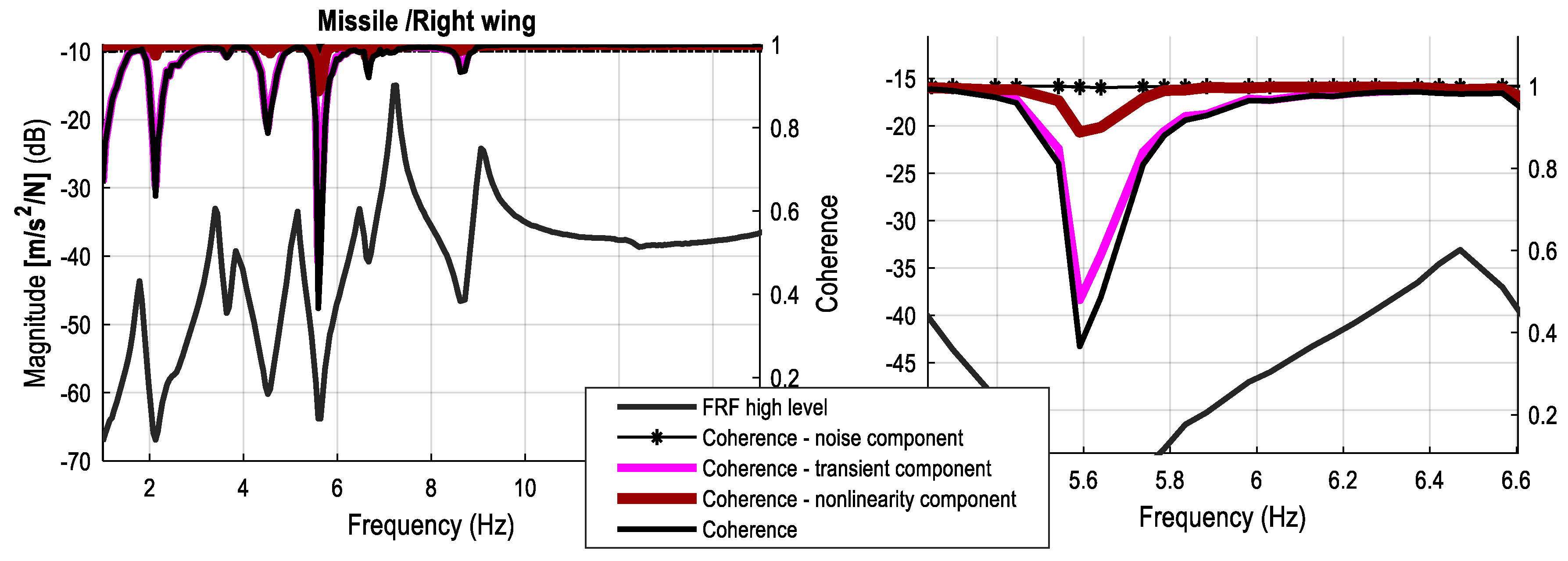
4.5.4. Coherence Function

Industrial practitioners tend to look at the (multiple) coherence function estimation [21] only, since the interpretation of the variances requires hands-on experience. When the coherence function gives one, it means that there is a 100% linear correlation between the measured output and input data. When the coherence is lower than one, it indicates the presence of (among others) high-level noise and/or transient and/or leakage and/or nonlinearities. Using the toolbox, the multiple coherence function estimate can be split up to noise, nonlinearity, and transient components.

Figure 14 shows the detailed coherence information. The analysis of this figure is very exciting. The coherence estimate with respect to the total measurement (thick black line) shows how many “imperfections” can be found in the measurement. When this coherence is split into components, one can see that the largest lack of coherence originates from the transient data (pink line). When an appropriate number of delay blocks are cut out from the measurement, this component is eliminated. The second largest lack of coherence contributor is the nonlinear component (red line). When an adequate nonlinear model is used, this component will be eliminated. The last component is the noise coherence component (thin black lines with asterisks), which tells us that the measurement quality was excellent.

The advantage of the variance technique over the coherence component technique is that different normalizations can be used; relative information is shown. For each pair of input–output, different variance levels are assigned. This restriction of the coherence component technique is related to the processing method (which is evaluated measurement-wise, experiment-wise).

5. Conclusions

In this work a novel automated MIMO BLA framework was developed to provide a user-friendly interpretation of the nonlinear behavior of MIMO measurement data by extracting user-relevant information. The toolbox turned out to be useful for modelling nonlinear FRFs because:

• It requires minimal user-interaction, and no expert-user
• Excitation signals are optimized for structures with multiple inputs
• The reference, input and output measurements were nonparametrically characterized
• The actuator system is characterized to improve the output measurement quality in case of nonlinear actuator and/or feedback
• An advanced frequency response matrix estimation method is used. It is a simple but robust estimation process; at each excitation level of noise, nonlinearity and transient information can be retrieved.

References

1. Kerschen, G.; Worden, K.; Vakakis, A.F.; Golinval, J.-C. Past, present and future of nonlinear system identification in structural dynamics. Mech. Syst. Signal Process. 2006, 20, 505–592. [Google Scholar] [CrossRef] [Green Version]
2. Worden, K.; Tomlinson, G.R. Nonlinearity in Structural Dynamics: Detection, Identification and Modelling; Institute of Physics Publishing: Bristol, UK, 2001. [Google Scholar]
3. Schoukens, J.; Godfrey, K.; Schoukens, M. Nonparametric data-driven modeling of linear systems: Estimating the frequency response and impulse response function. IEEE Control Syst. Mag. 2018, 38, 49–88. [Google Scholar] [CrossRef] [Green Version]
4. Schoukens, J.; Ljung, L. Nonlinear System Identification: A User-Oriented Road Map. IEEE Control Syst. Mag. 2019, 39, 28–99. [Google Scholar]
5. Lauwers, L.; Schoukens, J.; Pintelon, R.; Enqvist, M. Nonlinear Structure Analysis Using the Best Linear. In Proceedings of the International Conference on Noise and Vibration Engineering, Leuven, Belgium, 18–20 September 2006. [Google Scholar]
6. Esfahani, A.; Schoukens, J.; Vanbeylen, L. Using the Best Linear Approximation with Varying Excitation Signals for Nonlinear System Characterization. IEEE Trans. Instrum. Meas. 2016, 65, 1271–1280. [Google Scholar] [CrossRef] [Green Version]
7. Wong, H.K.; Schoukens, J.; Godfrey, K. Analysis of Best Linear Approximation of a Wiener–Hammerstein System for Arbitrary Amplitude Distributions. IEEE Trans. Instrum. Meas. 2012, 61, 645–654. [Google Scholar] [CrossRef]
8. Schoukens, J.; Pintelon, R. Study of the Variance of Parametric Estimates of the Best Linear Approximation of Nonlinear Systems. IEEE Trans. Instrum. Meas. 2010, 59, 3156–3167. [Google Scholar] [CrossRef]
9. Schoukens, J.; Vaes, M.; Pintelon, R. Linear System Identification in a Nonlinear Setting. Nonparametric Analysis of the Nonlinear Distortions and Their Impact on the Best Linear Approximation. IEEE Control Syst. Mag. 2016, 36, 38–69. [Google Scholar]
10. Pintelon, R.; Schoukens, J. System Identification: A Frequency Domain Approach, 2nd ed.; Wiley-IEEE Press: Hoboken, NJ, USA, 2012; ISBN 978-0470640371. [Google Scholar]
11. Csurcsia, P.Z. Static nonlinearity handling using best linear approximation: An introduction. Pollack Period. 2013, 8, 153–166. [Google Scholar] [CrossRef]
12. Heylen, W.; Sas, P. Modal Analysis Theory and Testing; Lirias: Leuven, Belgium, 2005. [Google Scholar]
13. Schoukens, J.; Pintelon, R.; Rolain, Y. Mastering System Identification in 100 Exercises; John Wiley & Sons: Hoboken, NJ, USA, 2012; ISBN 978047093698. [Google Scholar]
14. Csurcsia, P.Z.; Peeters, B.; Schoukens, J. The Best Linear Approximation of MIMO Systems: First Results on Simplified Nonlinearity Assessment. In Proceedings of the IMAC International Modal Analysis Conference, Orlando, FL, USA, 28–31 January 2019. [Google Scholar]
15. McKelvey, T.; Guérin, G. Non-parametric frequency response estimation using a local rational model. In Proceedings of the IFAC Symposium on System Identification, Brussels, Belgium, 11–13 July 2012. [Google Scholar]
16. Priemer, R. Introductory Signal Processing; World Scientific: Singapore, 1991; ISBN 9971509199. [Google Scholar]
17. Siemens, Simcenter Testlab. Available online: https://www.plm.automation.siemens.com/global/en/products/simcenter/ (accessed on 1 February 2020).
18. Kay, S.M. Modern Spectral Estimation: Theory and Application; Prentice Hall Signal Processing Series; Pearson Education India: Bengaluru, Indian, 1988. [Google Scholar]
19. Alvarez Blanco, M.; Csurcsia, P.Z.; Peeters, B.; Janssens, K.; Desmet, W. Nonlinearity assessment of MIMO electroacoustic systems on direct field environmental acoustic testing. In Proceedings of the International conference on Noise and Vibration, Leuven, Belgium, 17–19 September 2018. [Google Scholar]
20. Noël, J.P.; Schoukens, M. F-16 aircraft benchmark based on ground vibration test data. In Proceedings of the 2017 Workshop on Nonlinear System Identification Benchmarks, Brussels, Belgium, 24–26 April 2017. [Google Scholar]
21. Gómez González, A.; Rodríguez, J.; Sagartzazu, X.; Schumacher, A.; Isasa, I. Multiple Coherence Method in Time Domain for the Analysis of the Transmission Paths of Noise and Vibrations with Non-Stationary Signals. In Proceedings of the International Vibration and Noise Conference, Leuven, Belgium, 20–22 September 2010. [Google Scholar]
Figure 1. The structure of the best linear approximation (BLA, middle figure) and its connection to F-16 aircraft (left figure). GBLA refers to the BLA FRF, GE refers to standard deviation estimates of the noise, and Gs refers to standard deviation estimates of the nonlinear distortions.
Vibration 03 00007 g001
Figure 2. Evaluation of BLA estimate with the help of multidimensional averaging. Horizontally, the different period-wise FRF estimates G ^ [ m ] [ p ] can be found. A partial BLA estimate G ^ [ m ] and its improved noise estimate σ G ^ [ m ] 2 are obtained via the period-wise estimates. The BLA estimate G ^ B L A and its improved variance estimates σ ^ G ^ B L A 2 are obtained via partial BLA estimates (vertical direction). σ ^ N L 2 and σ ^ G ^ 2 stand for the improved (experiment-wise) stochastic nonlinearity and noise estimates. G S and G E stand for the period-wise stochastic nonlinearity and noise estimates (see Figure 1).
Vibration 03 00007 g002
Figure 3. Overview of graphical user interface (GUI) of SAMI. The displayed content is dynamic. The opening screen is shown on the left, where the user can import measurements, generate signals (see Figure 4), or open already existing projects. The middle figure shows the state when a measurement is loaded (imported): the user can choose to show the results of the analysis (see Figure 5), change basic graphical parameters (such as styles, see Figures 9–14), and save/export the results to Matlab or Siemens Testlab [17]. The third figure appears as an extension of the main interface when the user clicks on the setting button (see dashed circle): the details of the data segmentation and estimator parameters are displayed (concrete content is dynamic). Under normal circumstances the detailed view is hidden and the parameters are automatically set. Certain functionalities are illustrated in separated figures: (a)—Figure 4; (b)—Figure 5; (c)—Figures 9–14; (d)—Figure 8; (e)—Figures 6 and 8; (f)—Figure 6; (g)—Figure 12.
Vibration 03 00007 g003
Figure 4. Multisine generation module of SAMI. The left figure shows the opening screen of the multisine module where the default values are set from the user-defined profile. Under normal circumstances the user has to click on the generate figure only (the generated graphical output is shown the on the right). If the user has to overwrite the default parameters or opt for detailed design by clicking on the settings button (dashed circle), the GUI window is extended with the middle figure.
Vibration 03 00007 g004
Figure 5. Opening screen of an F16 MIMO measurement process. The contents (e.g., noise information, nonlinearities, warnings, number of tabs) are set by the user-defined profile and they vary dynamically. The grey/red shaded rectangular areas refer to the automated warnings of significant noise/nonlinearity level. Each of the figures can be double clicked such that in a new tab a detailed overview of the selected figure is given. Each of the tab’s elements can be saved as a regular Matlab figure (see Figures 9–14). In the measurement analysis tab a table/text based analysis is given.
Vibration 03 00007 g005
Figure 6. Structural testing of a small vehicle. It is excited vertically and horizontally. The right figure shows the FRF estimates: the black line is using 100 periods and the BLA estimator; the blue line is using 1 period and an H1 estimator; the red line is using 1 period and a Hanning windowed H1 estimator; the grey line is the automated choice of the toolbox, using 1 period. Observe that the automated choice (grey line) approximates the best of ideal (long) estimate (thick black line).
Vibration 03 00007 g006
Figure 7. F-16 ground vibration testing measurement campaign. The right wing is excited by a shaker; the voltage (reference) and force (input) signals of the shaker are measured. The major part of the nonlinearities is related to the payload connection interface where the acceleration is measured.
Vibration 03 00007 g007
Figure 8. Periodicity at the payload connection. The left figure shows the block repetitions (accelerometer data). The right figure shows the differences between the last block minus every block in dB scale. Observe in the second figure the fast decay in the first few seconds (this is the transient). The greyed area refers to the automatically detected transient (delay) block which will be discarded during the processing of the measurement. Please note that the automated transient check involves all available signals.
Vibration 03 00007 g008
Figure 9. The measured reference (voltage) and input (force) signals, and the FRFs of the actuator (shaker), are shown. Darker shades refer to higher excitation levels. Thick grey shades refer to the signals, FRFs. Thin grey shades refer to noise estimates. Orange shades (on signal measurements) refer to the odd distortions. Blue shades (on signal measurement) refer to the even distortions. Red shades (on FRF estimations) refer to (aggregated) nonlinear distortions. Observe that the higher the excitation, the more the nonlinear distortion on the output and FRF measurements.
Vibration 03 00007 g009
Figure 10. The output (acceleration) measurement shown at the payload connection. Darker shades refer to higher excitation levels. Thick grey shades refer to the signals. Thin grey shades refer to noise estimates. Orange shades (on signal measurements) refer to the odd distortions. Blue shades (on signal measurement) refer to the even distortions. Observe that the higher the excitation, the more the dominance of odd nonlinear distortions.
Vibration 03 00007 g010
Figure 11. The FRF estimation shown at the payload—right wing connection. Darker shades refer to higher excitation levels. Thick grey shades refer to the FRFs. Thin grey shades refer to noise estimates. Red shades refer to the nonlinear distortions. Observe that the higher the excitation: (1) the more the nonlinear distortions on the FRF measurements; (2) the lower the resonances; and (3) the higher the damping.
Vibration 03 00007 g011
Figure 12. FRFs, noise, and nonlinearity estimates shown at different normalization modes at a high level of excitation. Mode 0/1/2/3 refers to the block-wise/realization-wise/experiment-wise/nonlinear detection mode. Observe that the BLA FRF G B L A remains the same estimate. The noise and nonlinear distortion estimates are shown in case of normalization mode 0 with respect to one block; mode 1 with respect to one realization; mode 2 with respect to the whole experiment (all realizations). Mode 3 represents the nonlinear (variability) detection mode (where the nonlinearities are shown with respect to one block; noise is shown with respect to the all blocks). σ ^ N L 2 and σ ^ G ^ 2 stand for the improved (experiment-wise) nonlinearity and noise estimates. G S and G E stand for the period-wise nonlinearity and noise estimates (see Figure 1 and Figure 2).
Vibration 03 00007 g012
Figure 13. FRF, noise, and nonlinearity estimates are shown at low and high level of excitation using only one and all realizations.
Vibration 03 00007 g013
Figure 14. The BLA FRF estimation, coherence, and coherence components at high level of excitation; left—the whole frequency band of interest is shown; right—magnification of the figure is shown.
Vibration 03 00007 g014