Article

Friction-Induced Vibrations during Tightening of Bolted Joints—Analytical and Experimental Results

Workgroup on System Technologies and Engineering Design Methodology, Hamburg University of Technology, 21073 Hamburg, Germany
*
Author to whom correspondence should be addressed.
Vibration 2018, 1(2), 312-337; https://doi.org/10.3390/vibration1020021
Submission received: 25 October 2018 / Revised: 30 November 2018 / Accepted: 3 December 2018 / Published: 5 December 2018

Abstract

:
Bolted joints are one of the most used machine elements. Holding together structures of all sizes, the integrity rests on their shoulders. Thus, an accurate and reliable assembly of the joint is crucial. While it is the aim to not experience friction-induced vibrations at all, at some situations, it is unavoidable. These cases, however, have yet been out of the focus of control algorithms due to the volatile nature of the process. This contribution delivers analytical and experimental results for the occurrence of friction-induced vibrations during tightening of bolted joints. Previous findings of system characteristic constants could be validated, which can be used to monitor the tightening process even while strong vibrations during the tightening process occur. Additionally, a real-time algorithm is presented which allows for an advanced process monitoring and control by identifying process characteristics based on which predictions of the process can be made. These measures significantly improve the capabilities to reach the target values of the tightening process.

1. Introduction

Tightening bolted joints is ubiquitous in the assembly of machinery. With the goal to achieve the designed and required pretension force, the screw will be rotated by applying a torque in most cases. In practice, all motor parameters, like torque, angle of rotation, and angular velocity, are predefined by a protocol [1,2]. The control of the process is often limited to the motor controller, which follows the target values defined in the protocol [3]. Differentiating a good from a not good end state is key to achieve persistent high quality in serial production [4,5,6,7,8]. This is usually realized by predefining corridors for certain variables, like the tightening torque and the angle of rotation [9]. If these time-dependent corridors are passed correctly during the tightening process, it can be defined as error free. In all other cases, the assembly has failed, and the parts are eliminated form further processes. However, these control measures are effective only to a certain extent [10,11,12]. When major friction-induced vibrations occur during the tightening process, the torque- and angle-controller of the motor and the quality control mechanisms are prone to misjudge the circumstances due to insufficient knowledge about the frictional behavior [13,14,15]. This is one reason why it is generally advised to alter the process parameters in such a way that no friction-induced vibrations arise.
However, in some cases, e.g., with very large or very long screws at high loads, friction-induced vibrations are unavoidable [16], and thus a thorough understanding [17,18] has to be reached and a reliable control algorithm needs to be found in order to achieve high quality joints and reliable assembly processes. The presented algorithm solves three needs for tightening processes experiencing friction-induced vibrations: monitoring the quality of the process, increasing the motor control of the process, and evaluating the increased load on the tools.
This contribution investigates the tightening process using an analytical approximation for the dynamic process, which supplements previous findings of numerical simulations [19]. Furthermore, experiments of typical assembly situations are performed, and the stick-slip phenomenon is recorded and compared with analytical data. Lastly, an algorithm for a real-time prediction of the stick-slip events is presented. This algorithm significantly reduces the uncertainty the analytical solution inevitably possesses and allows for predictive maintenance of the apparatus.

2. Stick-Slip in Bolted Joints

The tightening of bolted joints is characterized by an increase of the pretension force F due to the rotation of the thread by the angle φ th . Because the angle of rotation during tightening is a function of time t, the pretension force becomes a function of time, too:
φ t T F .
These factors are related by the torque T that is applied at the bearing of the screw and increases over time, thus rotating the screw. This assumption can be made based on the fact that the starting point of a friction-induced vibration is statistically distributed and macroscopically, the variables become linearly dependent.
Applying a constant torque would eventually stall the motor and lead to stiction of the friction surfaces. Thus, it is necessary to control the torque adequacy in order to control the motion of the system. The system is prone to experience friction-induced vibrations due to the ever increasing preload force and torque necessary to further rotate the screw. The alternation of stiction and sliding leads to a number of impulses and is called stick-slip. This phenomenon has been studied in many fields [20,21,22], but little has been done in the field of controlling tightening of bolted joints.

3. Analytical Model

One contributor for the occurrence of stick-slip is a significant difference between the friction coefficients for stick and slip [20,21,23]. In order to derive an estimation of the occurrence of stick-slip during tightening of bolted joints, the screw is assumed to be ideally stiff. This reduces the two frictional contacts of the bearing and the thread to a single contact. The reduction of complexity can also be argued with the fact that in the macroscopic view, the friction torque is independent of the contact area. Considering the bearing and thread friction contacts possessing very similar surface properties, changing just the contact area does not make a difference in a first approximation.
In our analytical model, the Coloumb friction model is chosen by using the two coefficients of friction μ stick and μ slip in order to differentiate between the two major states of sticking and sliding. The simplified model is depicted in Figure 1.
It consists of an ideal torque source with the constant angular velocity φ m , an extension from the motor to the screw with length l e and diameter d e , a screw with a bearing contact radius r and an effective shaft length of l s , as well as the clamped parts and a nut, which is ideally connected to the plates.
Although an extension is technically not required, in a lot of tightening cases, it is necessary in order to reach the joint position. The torsional stiffness k e of the drive train has a significant effect on the dynamics of the system. It can be approximated by
k e = G · J p l e = π 32 · G · d e 4 l e ( Nm ) with J p = π 32 · d e 4 ( m 4 ) ,
where G denotes the shear modulus of the material and J p the polar moment of inertia of the extension.
With the motor transferring the torque to the head into the bearing of the screw, the latter will be rotated and increase the pretension force onto the clamped parts [24,25,26,27]. The frictional contact area underneath the bearing is approximated by [28]
r = 2 3 · r b , min · γ 2 + γ + 1 1 + γ with γ = r b , max r b , min .
The pretension force can be approximated by the angle-, respectively time-dependent function F ( φ th ) F ( t ) . Under the assumption that the effective shaft length of the screw l s is increased during the tightening process, the distance Δ l s is defined by the rounds the thread is rotated multiplied with the pitch P of the screw:
Δ l s = φ th · P .
The pretension force F can be derived following Hook’s law with the Young’s modulus E and the cross-section area A of the shaft:
F = Δ l s l s · E · A ,
A = π · d 2 4 ,
where d denotes the nominal diameter of the screw. Assuming an ideal stiff screw, the angle of the thread φ th and the bearing angle φ b should remain the same:
φ th = φ b .
The stiffness of the screw can be abbreviated by the factor k s :
F = φ b · k s with k s = P · E l s · π · d 2 4 .
The pretension force F induces a frictional reaction torque T, which is also the motor torque, based on the surrogate friction radius r and the coefficients of friction μ stick and μ slip , that is opposite of the acting torque due to the twist of the extension and its torsional stiffness. The torque which the screw experiences depends on the difference of the motor angle φ m = φ m ( t ) , the angle of the stiff screw φ b = φ th ( t ) , and the stiffness k e of the extension, which connects the motor to the screw head:
φ ˙ b = 0 T = ( φ m φ b ) · k e F · r · μ stick = T stick ,
φ ˙ b 0 T = ( φ m φ b ) · k e = F · r · μ slip = T slip .
Hence, the reaction torque depends on the frictional state.

3.1. Phases of Stick-Slip Motion

In order to describe stick-slip motion, the dynamic process is separated into two phases: sticking phase and sliding phase. Both phases can be solved independently if the start and end constraints are well-defined. The sum of both durations defines one period of a stick-slip event. However, due to the fact that the sliding phase will be orders of magnitude shorter than the sticking phase, the duration of the sliding phase is assumed to be zero in our analytical model. With Equations (9) and (10), distinct states of the dynamic process can be defined. These states correspond to angles of the system.
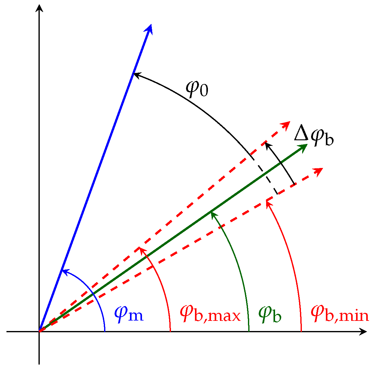
The minimum and maximum values of the screw angle φ b are coupled with the motor angle φ m by γ stick and γ slip (see Figure 2). Thus, the screw angle stays stationary while φ m as well as φ b , max and φ b , min increase over time until φ b = φ b , min . Then, one slip event is initiated due to change from stiction to sliding friction, and the screw angle φ b rotates to φ b , max . The passed angle is Δ φ b . In order to derive the torque limits at the points just before and just after the switch from stiction to sliding, we use the following equations to derive an approximation of the angle of rotation of the screw φ b :
( φ m φ b ) · k e = F · r · μ i ,
φ m · k e φ b · k e = F · r · μ i ,
φ m · k e = φ b · k e + F · r · μ i introduce Equation ( 8 ) ,
φ m · k e = φ b · ( k e + k s · r · μ i ) ,
φ b = φ m · k e k e + k s · r · μ i ,
φ b , min = φ m · γ stick with γ stick = k e k e + k s · r · μ stick ,
φ b , max = φ m · γ slip with γ slip = k e k e + k s · r · μ slip .
With the torque states defined, both phases can be investigated separately, as is described in the following.

Sliding phase

At the beginning of the sliding phase, the drive train is twisted and pretensioned to the point at which the current torque has just surpassed the sticking torque, T T stick [see Equation (9)]. With the knowledge of the motor rotation φ m , the rotation of the screw φ b , and the pretension force F, we see that Equation (9) is true during the sticking phase, but just until the torque in the extension is equal to the stiction torque of the screw. In that moment, the friction coefficient will switch from stiction to sliding friction and thus be reduced by Δ μ = μ stick μ slip . During the following sliding phase, the screw will rotate rapidly by Δ φ b until the torque in the extension equals the sliding frictional torque, this is the minimum angle:
Δ φ b = φ b , max φ b , min .
Simultaneously, the torque in the extension has decreased by Δ T , and the pretension force has increased by Δ F .
The maximum angle, that the bearing can rotate towards the motor, is the difference between the current angle of the motor φ m and φ b , min , respectively φ b , max :
φ 0 , stick = φ m φ b , min ,
φ 0 , slip = φ m φ b , max .
Being able to quantify the slippage of the screw during every event, the boundaries for the torque drop Δ T and the force step Δ F can be derived as follows:
Δ T min = Δ φ b · k e ,
Δ T max = φ 0 , stick · k e ,
Δ F min = Δ φ b · k s ,
Δ F max = φ 0 , stick · k s .
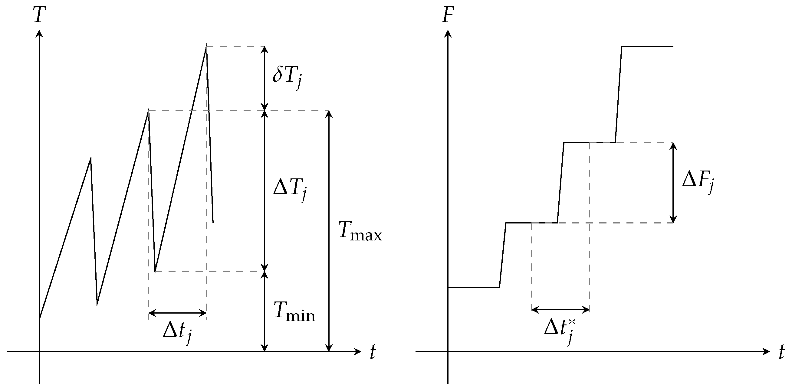
The corresponding process metrics are defined in Figure 3.

Sticking phase

During the sticking phase, the screw stands still while the drive train is rotating by the motor’s constant angular velocity φ ˙ m . The extension of length l e is therefore experiencing torsional stress, which in turn results in an increase of torque at the screw. The torque will increase as long as the frictional torque T stick F · r · μ stick is not overcome. Due to the fact that the screw has just passed the previous sliding phase, it has rotated by an angle between the stated boundaries and is partially relaxed. The time the motor needs to catch up with the just rotated angle during the slipping phase defines the frequency of the next stick-slip event:
f ss , min = φ 0 , stick φ ˙ m 1 = φ m φ b , min φ ˙ m 1 = t · φ ˙ m · ( 1 γ stick ) φ ˙ m 1 = 1 t · 1 1 γ stick ,
f ss , max = Δ φ b φ ˙ m 1 = φ b , max φ b , min φ ˙ m 1 = t · φ ˙ m · ( γ slip γ stick ) φ ˙ m 1 = 1 t · 1 γ slip γ stick .
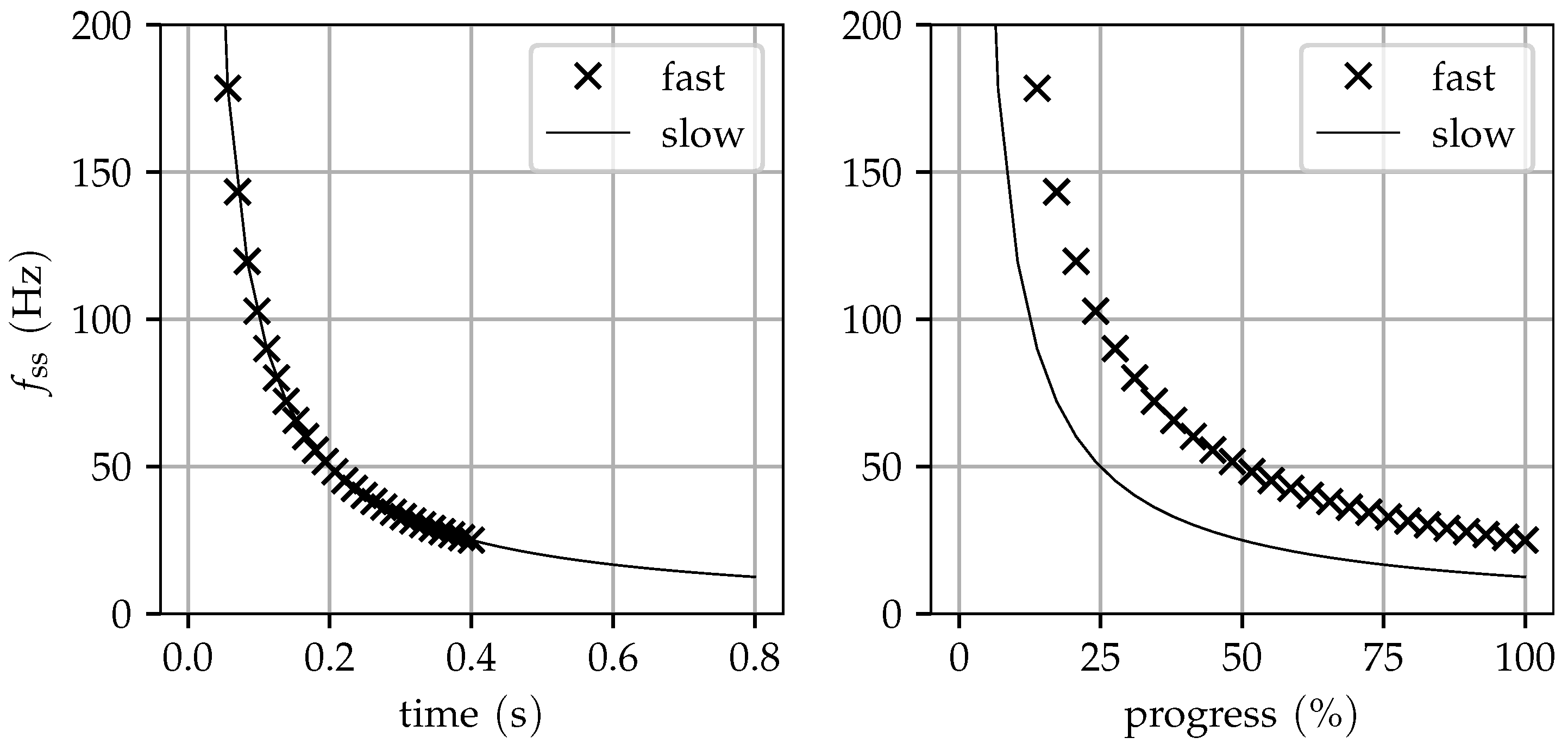
It is notable that Equations (25) and (26) are absent of a dependency of φ ˙ m . This is counterintuitive because with the increase of the tightening velocity, the frequencies should also increase. However, considering the angular velocity φ ˙ m being constant, the total process time t total until the maximum tightening torque T max is reached is known. With a higher angular velocity, the entire process is completed in a shorter time. Hence, while following the same frequency curve, processes with different angular velocities experience different frequencies relative to the progress of the tightening process (see Figure 4).
So, overall, the frequencies are higher than with a higher φ ˙ m .

3.2. Approximation of Tightening Time

The total process time t total can be estimated by adding the time it takes to twist the extension t e and the time it takes to pretension the screw t screw :
t total = t e + t screw ,
t e = T target φ ˙ m · k e ,
t screw = F target φ ˙ m · l s P · E · 8 d 2 .
The following approximation can be used to derive either T target or F target :
T target = F target · P 2 π + d 2 3 · μ th + D b 2 · μ b .
This torque–pretension force relationship known from Kellermann and Klein [29] and VDI 2230 [1] has proven itself to be sufficiently accurate in practice. It can be used to define a target torque or a target pretension force and derive the other.
Given a screw that was chosen based on the design purpose and the goal to achieve a high assembly speed, the only left option to alter the stick-slip frequencies during tightening is to choose an appropriate extension. The higher the stiffness of the extension, the higher the stick-slip frequencies. Thus, the increase of the diameter d e has a significant influence. Less sensitive, but probably more easily adaptable, is the length l e of the extension, which only has a linear influence. Shortening the extension results in a higher frequency and thus in a smaller uncertainty of the end-state of the tightening process.

3.3. Characteristic Constants

The macroscopic linear relationship of the variables of the tightening process and the linear Couloumb friction model results in regular vibrational patterns. Baramsky et al. [19] have defined three constants that describe this behavior. The stick-slip frequency f ss over time can be described by the constant K 1 , the step increase of the pretension force in relationship to the duration of the stick period by K 2 , and the torque drop at a given time by K 3 :
K 1 f ss · t ,
K 2 Δ F Δ t · φ ˙ m ,
K 3 Δ T t · φ ˙ m .
These constants can be approximated using the analytical equations above:
K 1 , min 1 1 γ stick ,
K 1 , max φ b , max φ b , min φ ˙ m 1 · t ,
K 2 , min Δ φ b · k s Δ t · φ ˙ m = Δ φ b · k s · f ss · φ ˙ m ,
K 2 , max Δ φ 0 , stick · k s Δ t · φ ˙ m = Δ φ 0 , stick · k s · f ss · φ ˙ m ,
K 3 , min Δ φ b · k e t · φ ˙ m ,
K 3 , max Δ φ 0 , stick · k e t · φ ˙ m .
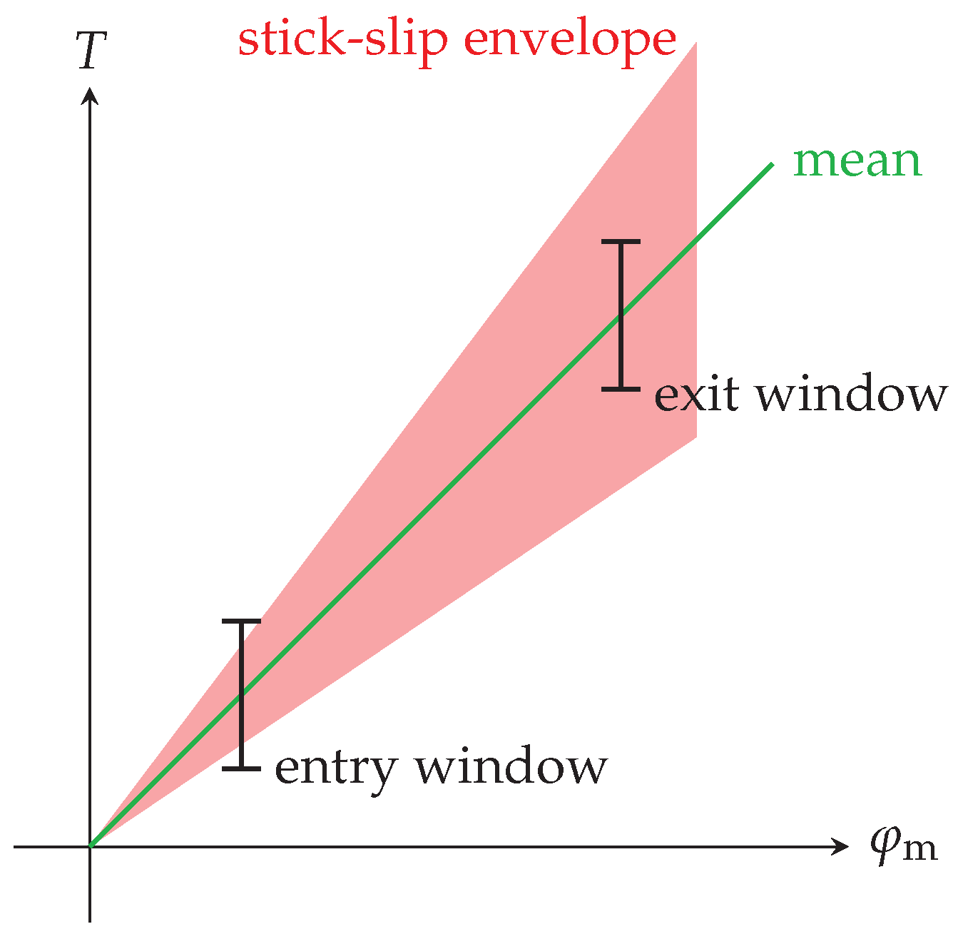
Commonly, tightening processes are supervised by monitoring the tightening torque and motor angle and defining windows in the data frame, which have to be passed correctly in order to define a process as error free. With tightening processes that are subject to intense friction-induced vibrations, these windows are of little help. Because of the high variance of the torque values, no steady mean value exists that could pass the window consistently. This is illustrated in Figure 5.
The windows could be enlarged, but that defeats the purpose of a control window. Hence, other metrics must be used to monitor the process quality. The constants K 1 to K 3 can be used for that purpose. They deliver values that will be constant over the time of the process for every specific joint. Their values correspond to the three major monitored data types: time ( K 1 ), pretension force ( K 2 ), and motor torque ( K 3 ).

3.4. Dependency of Geometric Features on Stick-Slip Vibration

The main contributors for friction-induced vibrations are the stiffness of the extension k e , the stiffness of the screw k s , and the friction coefficients μ stick and μ slip . These factors are dependent on their respective geometric features (see Figure 6).
The spectrum of common combinations of lengths and diameters for DIN screws shows the corresponding characteristics with the derived screw stiffnesses k s so that a meaningful interval of k s = [ 30 , 180 ] kN was chosen. Typical extension lengths are between 50 and 500 mm with a diameter between 8 and 15 mm, which results in an interval of k e = [ 200 , 2000 ] Nm . The two factors γ stick and γ slip can be calculated over that spectrum. If not changed to demonstrate the dependencies, the further used parameters are G = 81 GPa, E = 210 GPa, ρ = 7900 kg m 3 , P = 1.5 mm, d o = 29 mm, d i = 15 mm, l s = 85 mm, d = 14 mm, μ stick = 0.2 , μ slip = 0.15 , l e = 200 mm, d e = 10 mm. Here, ρ describes the density of the screw material, and d o and d i are the outer, respective inner diameter of the screw’s bearing surface.
The bearing rotation Δ φ b is significant for the calculation of the stick-slip frequency, the torque drop, and the force step, see Equation (18). This is based on the difference of γ slip and γ stick . As long as the difference between the two friction coefficients is small, the factor stays relatively small too (see Figure 6). The smaller the difference between the friction coefficients, the higher the frequencies.

4. Stick-Slip Due to Resonance

An obvious assumption is to take the resonance of the drive train as a relevant factor of friction induced vibrations into account. With the drive train and joint being elastic bodies, resonance frequencies and motion-modes exist. Based on the fact that the drive train has to come to a full stop at the end of the tightening process and thus all motions that could vibrate in resonance become slower, the modes with the lowest natural frequency at the end of the tightening process are the most important ones. Typically, two sources of relatively low natural frequencies can be identified: the shaft of a (long) screw and the (long) extension of the drive train. In addition to that, during the phase of plastic deformation of the screw, the pretension force remains relatively constant and thus the constraints too, which results in a relatively constant rotational stick-slip frequency. This frequency is driven by the state of the joint and the dimensions of the drive train. The former can be described by the effects discussed in the sections above. The latter has an influence when the stick-slip frequency is near a natural frequency of the drive train.
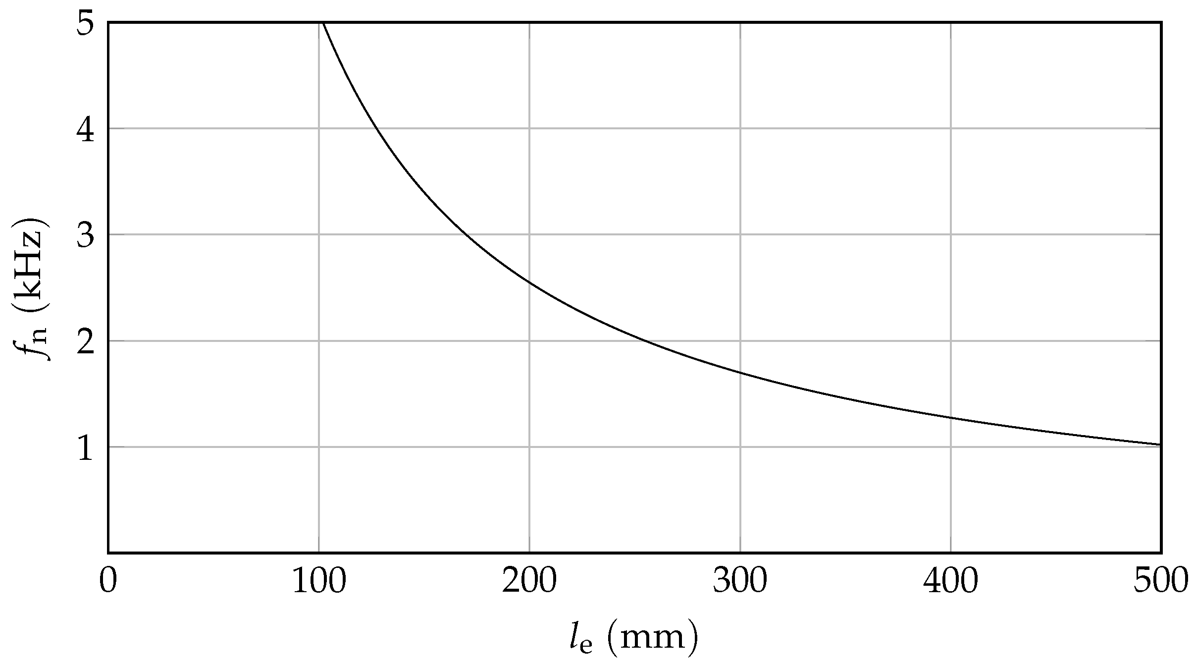
Both effects share the phenomenon that the vibration frequency stays relatively constant for the duration of the respective effect in comparison to the stick-slip phenomenon due to the increase of pretension force. The natural first-order rotational frequency of a cylindrical body with the length l e , density ρ , and shear modulus G can be derived as
f n = 1 2 π G l e 2 · ρ .
In the case when the stick-slip frequency and the natural frequency of the drive train are overlapping, the state of vibration can become dominant for the rest of the process. This has been investigated in some cases [30]. However, this coincident is very unlikely due to the different frequency spectra. Considering an extreme case, the derived frequency of a 500 mm long extension is greater than 1 kHz, which is very high compared to the measured stick-slip frequencies (see Figure 7). Thus, the interference of both frequencies is very unlikely. It remains open if any bending mode of the extension, which has a significant lower first-order natural frequency, can have an influence on the friction-induced vibrations. However, because of the induction of local surface pressure due to the bending of the nut at the head of the screw, an analytical study is not possible [31]. The superposition of multiple vibration modes can only be simulated numerically, but will stay out of the scope of this paper. Most screws are made of steel and thus share very similar properties with the extension of the drive train, with the result that they also share the natural frequencies shown in Figure 7.
Only screws with extremely long shafts over 500 mm will come near the frequencies that occur during the tightening process. In conclusion, it can be said that any resonating vibration based on the first-order rotational natural frequency can practically be neglected.

5. Experiments

The tightening process has been investigated on a test rig by Kistler (former Schatz AG, Remscheid, Germany). The rig consists of the torque source Schatz 2413-4119 with a maximum torque of 1000 Nm, a sensor for the angle of rotation Schatz MOD 5413-1200/200-S, and the torque and pretension force sensor Schatz 1961A (100/150). The data are recorded with a frequency of 1000 Hz with the software testXpert by Zwick/Roell, (Ulm, Germany) and post-processed with MATLAB by The MathWorks, Inc., (Natick, MA, USA) and Python 3.5.
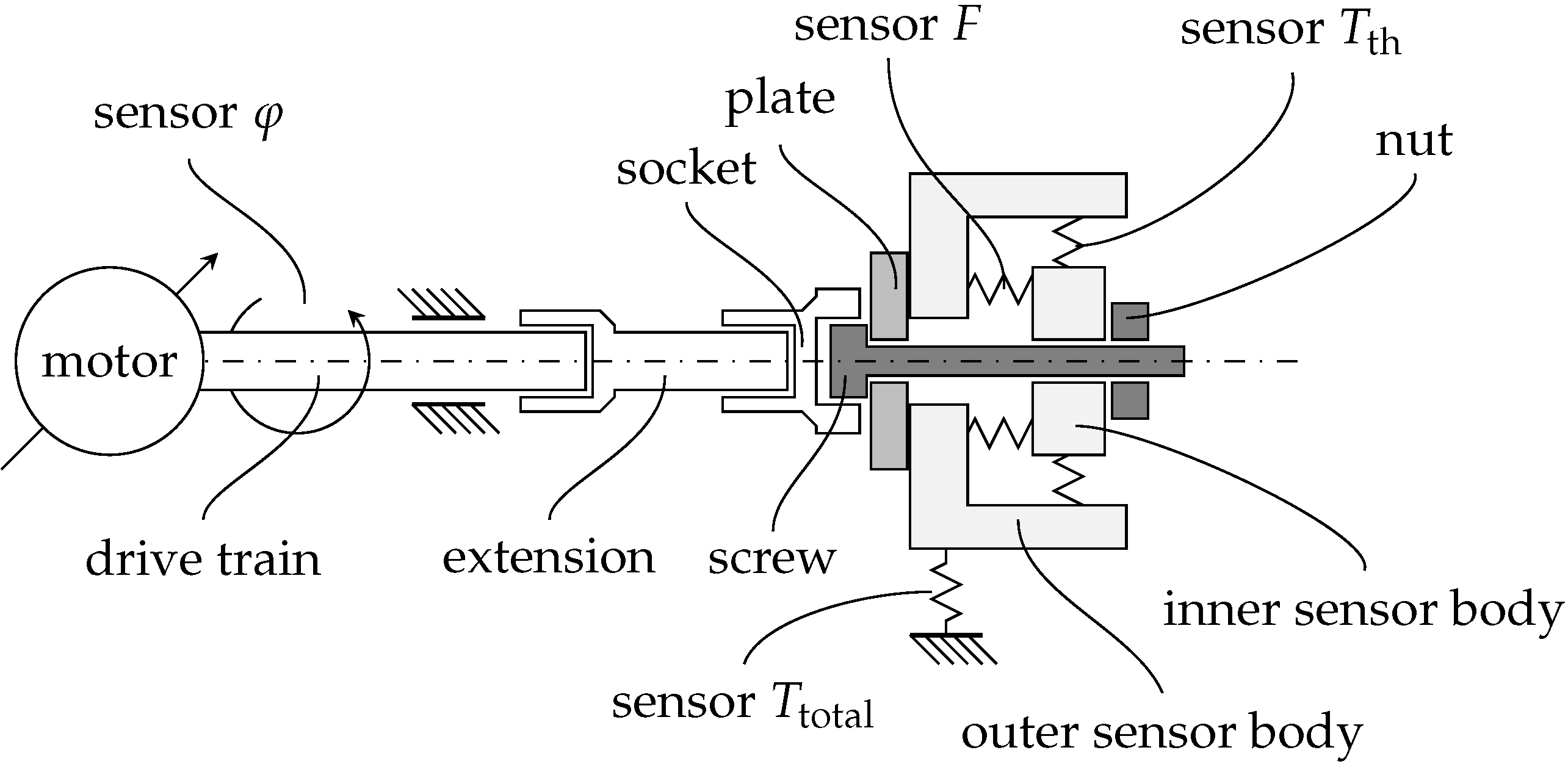
The torque is introduced by a servo motor with a high gear ratio followed by a stiff drive train on which a torque and an angle sensor are attached (see Figure 8).
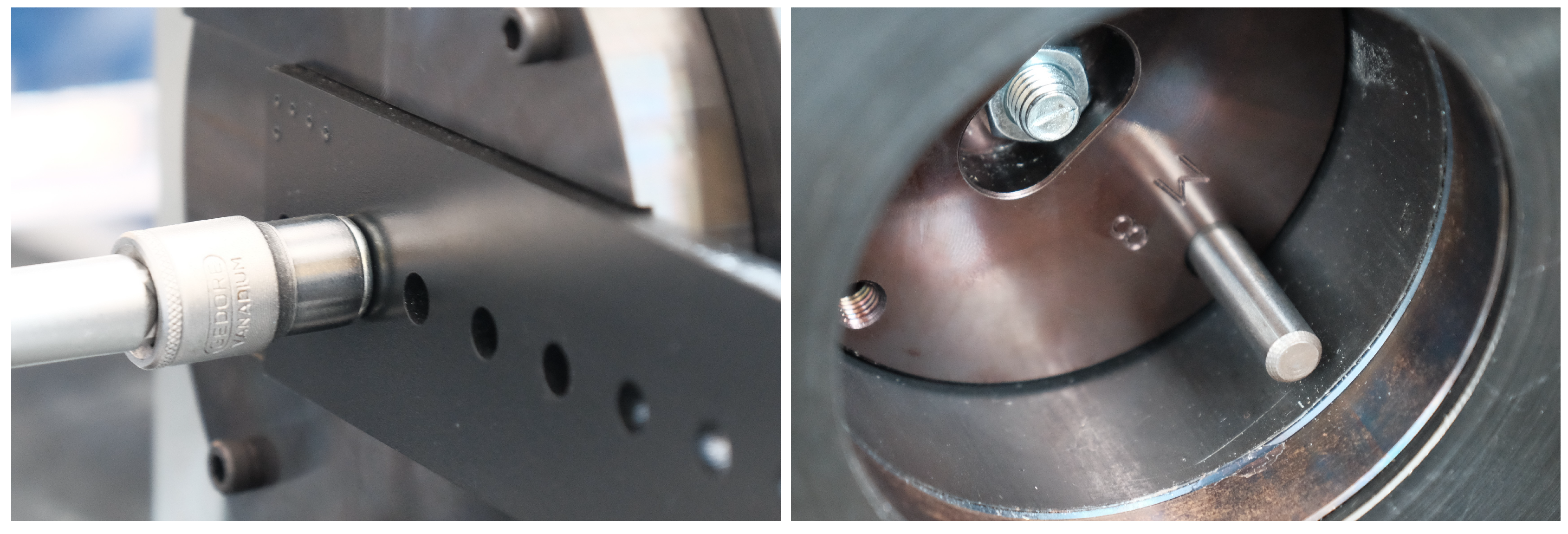
The drive train is connected to an extension, which itself is attached to a socket at its end. The socket introduces the tightening torque onto the hexagonal screw head which is bolted into the sensor apparatus. The sensor apparatus consists of two main parts: the outer sensor body, which holds the plate the screw head is pressed onto, and the inner sensor body, which grasps the nut. Both bodies are connected by two sensors utilizing strain gauges in order to measure the pretension force F and the thread torque T th . The outer sensor body is also connected to the ground in order to measure the total torque T total . Adapters for the plate and nut as well as for the clamping distance allow for a versatile adjustment of a multitude of screws and bolts (see Figure 9). The sensors of the test rig allow for recording the following parameters: motor torque T m , motor angle of rotation φ m , total torque T tot , thread torque T th , and pretension force F. Based on these parameters, the bearing torque T b = T total T thread and motor angular velocity φ ˙ m = d φ m d t can be calculated.

5.1. Specimen Preparation and Conduction of Test Runs

Cathodic dip coating and steel screws were chosen because this is a common combination in the automobile industry in load-bearing body construction. The blank steel specimens are stored at room temperature with a slight coat of oil to prevent rust. All tests are performed at room temperature with the machine and specimens at an identical temperature. The screws and nuts were cleaned with isopropanol using a three minute ultrasonic bath with a technical cleaning fluid. The clamped plates were wiped with a cloth and isopropanol. Afterwards, everything is handled with silicone gloves to prevent any contamination with lubricants. For the experiments, M14 10.9 metric screws with a flange length of 100 mm and a pitch P = 1.5 mm were used. The clamping distance (effective length of the shaft l e ) was varied from 55 to 85 mm. The tightening velocity φ ˙ m varies from 1 to 150 rpm. The extension from the torque source to the socket l s was changed from 110 to 350 mm. A typical test with a significant stick-slip phenomenon was chosen to demonstrate the capabilities of the analytical representation and the process of prediction.

5.2. Test Results and Comparison to Analytical Data

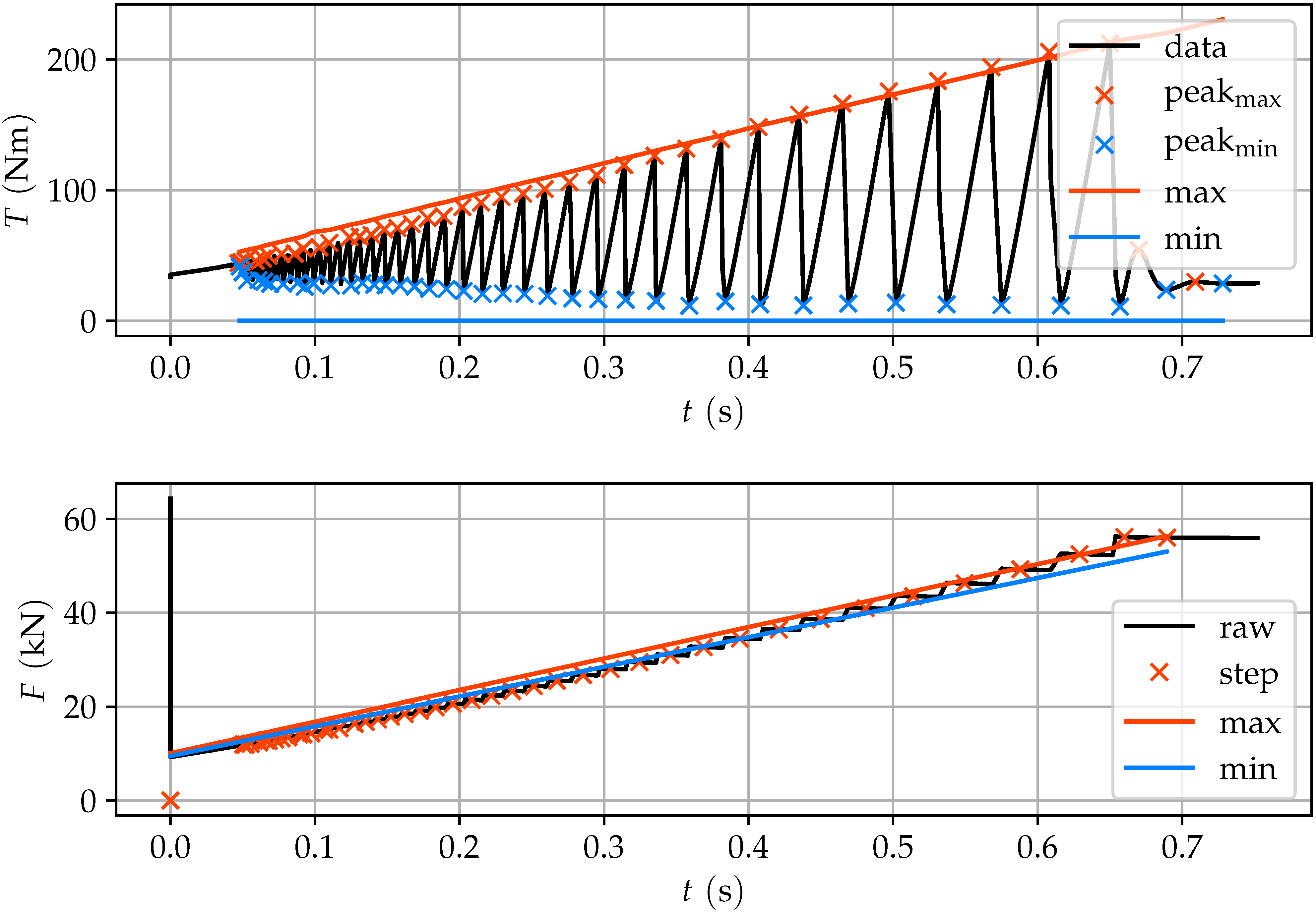
The analytical model presented in Section 3 approximates the experimental values very closely (see Figure 10).
All parameters for the analytical calculations are taken from the experimental setup; material parameters: shear modulus G = 81 GPa , Young’s modulus E = 210 GPa , density ρ = 7900 kg / m 3 ; screw parameters: pitch P = 1.5 mm , outer diameter of the bearing surface d o = 29 mm , inner diameter of the bearing surface d i = 14 mm , basic pitch diameter d 2 = 12.6 mm , length of screw shaft l s = 85 mm , diameter of screw shaft d = 13 mm ; extension parameters: length of extension l e = 110 mm , diameter of extension d e = 10 mm ; process parameters: angular velocity of motor φ m = 0.5 s 1 , target torque T target = 200 Nm , target pretension force F target = 56 kN . The coefficients of friction μ stick = 0.38 and μ slip = 0.35 were identified through the measured data. The relationship between the applied torque and the resulting pretension force is strongly based on the inhibiting friction of the screw. These values can be determined early during the process. Based on the analytical model, μ slip has to be very close to μ stick in order to reproduce the observed behavior. The norm DIN 16047 [5,29] suggests a total friction coefficient μ total = 0.18 for steel-on-steel:
μ total = T target F target P 2 π d 2 3 + r = 0.18 .
However, this does not account for the dynamics of the stick-slip phenomenon with the chosen material and coating combination, and describes a scenario with sole sliding friction. A simple approximation reveals a friction coefficient of about μ * = 0.32 , which corresponds with the identified values above:
μ * = T target F target · r = 0.32 .
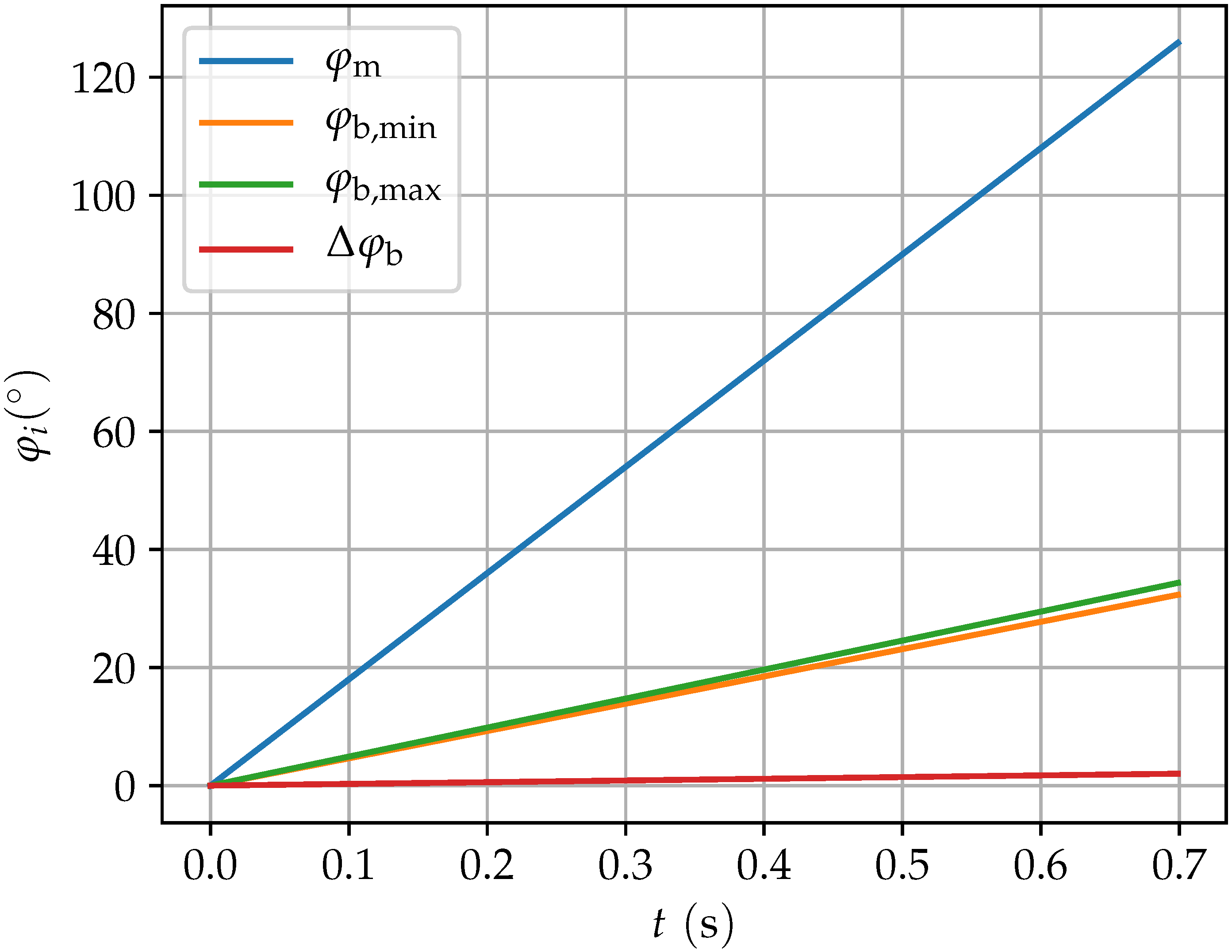
For demonstration purposes, the start point of the raw data of Figure 10 is chosen to be at F = 10 kN . Before that, nonlinear setting processes happen. First, friction-induced vibrations occur at around 0.05 s. Before that point in time, the algorithm would not detect any peaks, and the regular control system of the tightening process would take care of the motor torque and angle. Furthermore, the end of the process is shown as the torque does not reach another big peak after 0.65 s. The tightening process was set to stop at a pretension force of F target = 56 kN and was capable of releasing the torque at the motor within a millisecond. This demonstrates the capability to reliably stop the tightening process when the real-time prediction recommends a stop of the process. In most tightening scenarios, it is mostly only possible to measure the motor angel. The analytical equations allow for a deeper insight (see Figure 11), based on the angles introduced in Figure 2.
The analytically estimated maximum and minimum values of the torque (see Section 3.2) show a close approximation of the raw data (see Figure 10). With the maximum slip angle of the screw being the angle of the motor, where the extension is not twisted, the minimal reached torque is 0 Nm. Due to backlash and setting processes in the drive train, the start of the experiment does not correspond with the start of the simulation time. Hence, a time shift of 0.15 s was introduced to ensure comparability.
The magnitude of the step-like increase of the pretension force depends decisively on the discharge of the potential energy stored in the drive train during a slip event and thus on the frictional behavior. Reasons for the partial stress relief can be the quality of the surface between the bearing of the screw and the surface of the clamped part. A small surface disturbance can lead to a short stop, switching back the friction condition to stiction. The cathodic dip coating changes its influence during the tightening process due to abrasive wear, with the particles of the coating stying in the contact area (see Figure 12).
Further reasoning for a partial relief can be found in the fact that the screw itself is an elastic body and a rotation of the head does not mean an equal rotation of the thread, which in turn pretensions the screw. For the purpose of simplicity, the tightening process was reduced to a single elastic body. A more sophisticated multi-body model has been presented in [19].

5.3. Frequency

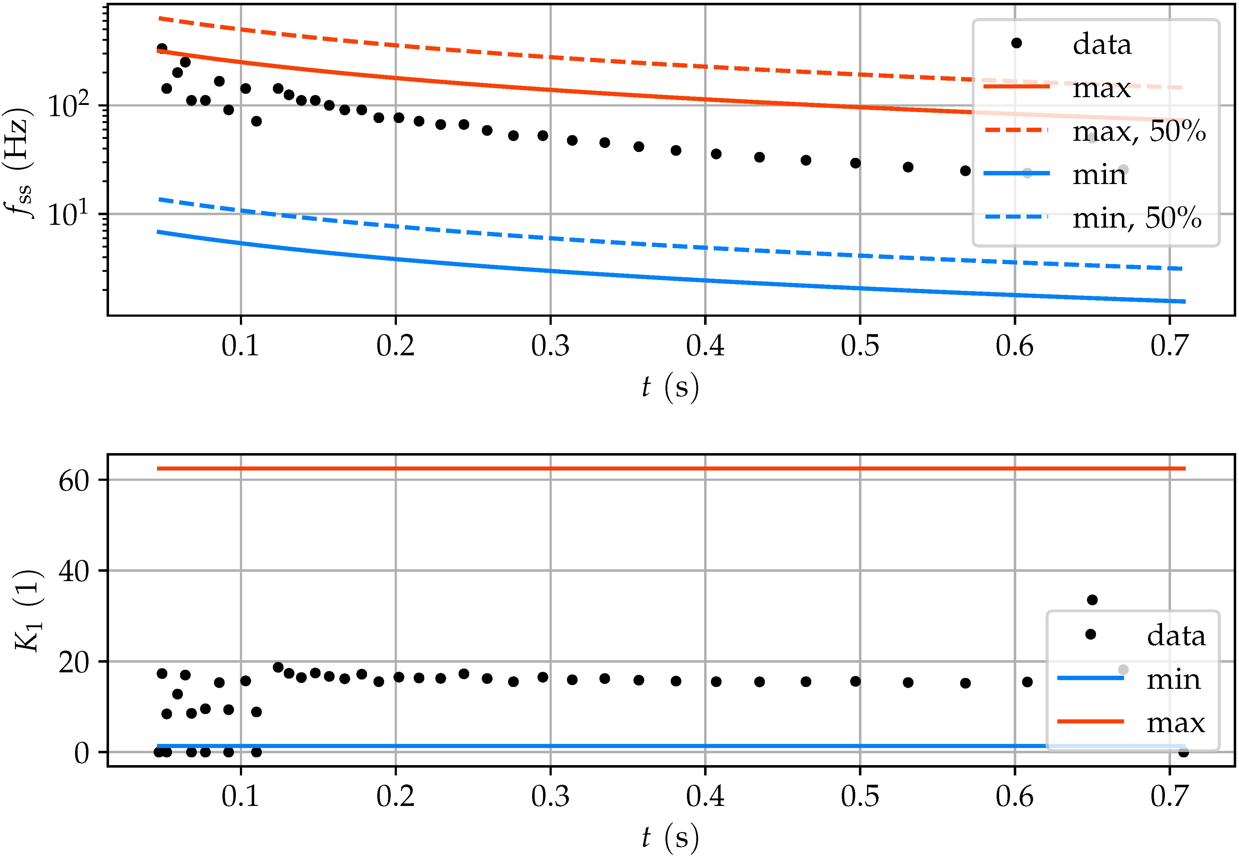
The frequency is analytically estimated with good precision (see Figure 13).
The solid lines describe the expected frequency barriers derived from Equations (23) and (24). The dashed lines demonstrate the frequency if the potential energy that was stored in the system was only released by 50% and thus, the screw is rotated only half as much. Consequently, the time it takes to reestablish the torque to trigger the next slip event is about halved, resulting in a higher frequency. It is notable that the recorded data of the frequency is noisy in the first two hundred seconds. Afterwards, it follows a very regular pattern. The last two data points show the end of the tightening process. Here, the evaluation also has ended. The constant K 1 approximates the actual data in a good manner. The expected maximum and minimum values envelope the experimental data. The data appear to show a very constant behavior.

5.4. Pretension Force Step

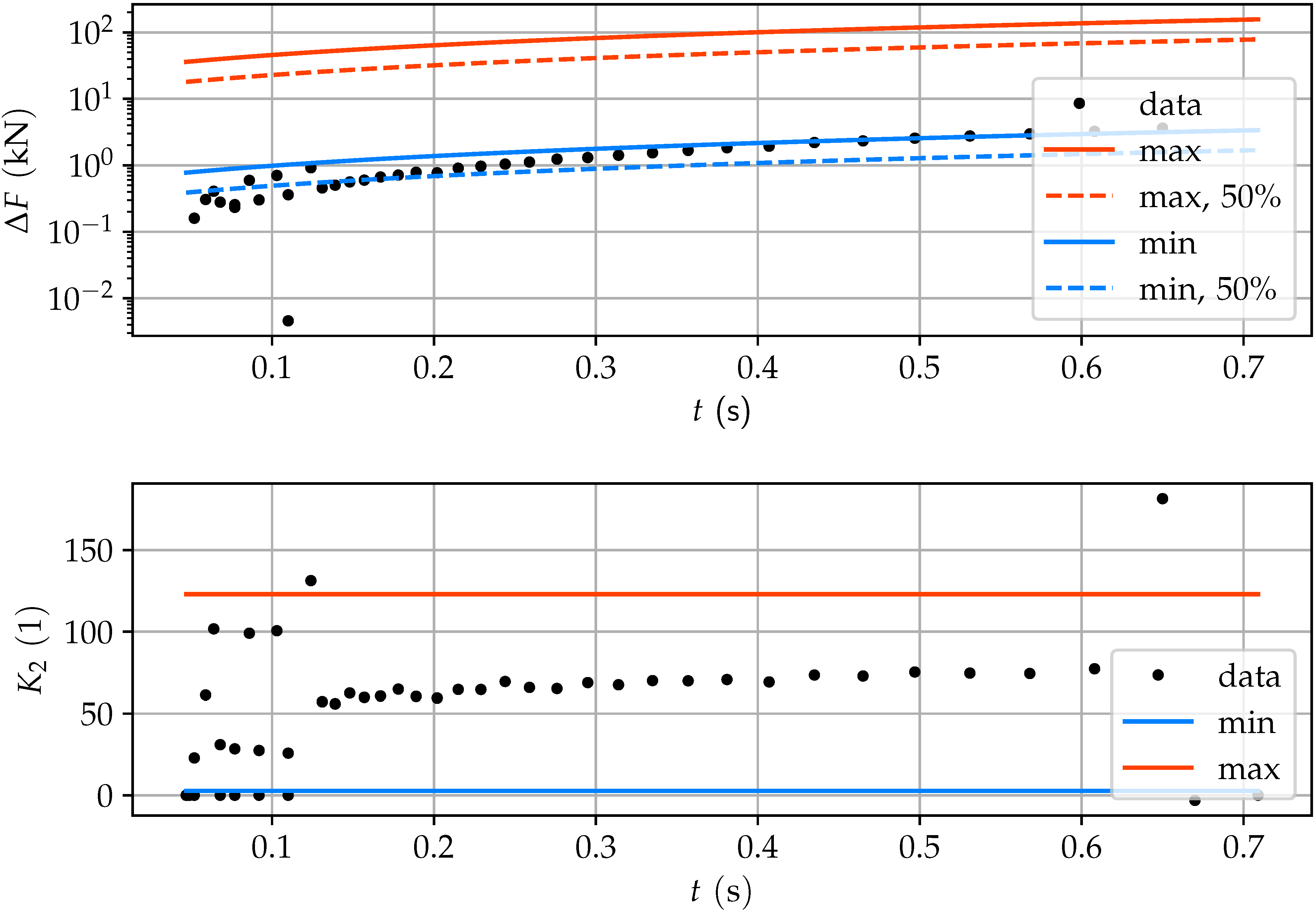
The force steps of the experimental data are on the lower spectrum of the analytical estimation (see Figure 14).
This signalizes that the potential energy stored in the extension is only partially converted into the pretension force of the screw. The analytical approximation can be extended by taking into account that the shaft of the screw is an elastic body, too. The dashed line represents the effect of a partial (50%) release of energy, as explained above. Another reason for a lower than expected force step could be backlash in the real system. Whereas the model considers/assumes ideal connections, in contrast, the real world test rig does have some degree of backlash. Nonetheless, the analytical approximation delivers usable boundaries for Δ F . The constant K 2 shows very consistent data within the boundaries in a linear manner.

5.5. Torque Drop

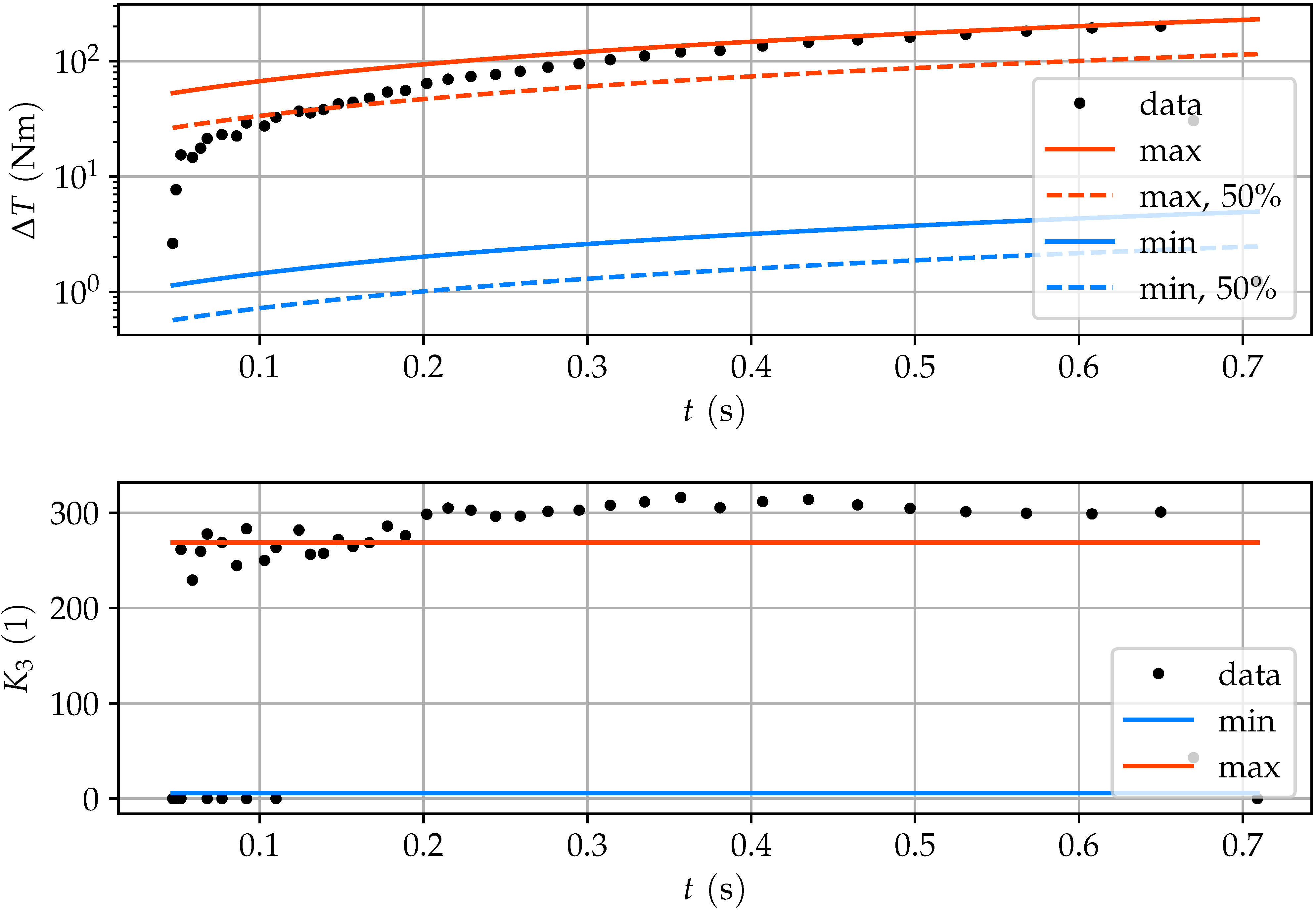
The torque drop is recorded to be at the upper boundary of the analytical approximation (see Figure 15). This can be also explained by the backlash in the drive train: the rotation of one slip event is great enough to rotate the drive train, or parts of it, into a contactless position. Inertia distribution and backlash positions in the drive train are crucial. A loose socket eases the contact of the tool to the screw head, but also introduces dynamic disadvantages during friction-induced vibrations. The constant K 3 shows what is expected due to the backlash: a higher torque drop per time. However, the approximation is in unison with the data.

6. Real-Time Prediction

An analytical estimation supports the design of the parameters for the tightening process and allows to analyze the dependency of certain factors like geometry and material properties. However, in order to adequately control the process in real time, the analytically obtained estimates are not sufficient. Therefore, an algorithm for a real-time prediction of the near future of the process is introduced in the following. Tightening processes can take from fractions of seconds to minutes, depending on the size of the joint and the tightening strategy. Being able to reliably calculate the current process status and derive good decisions about the process can only be achieved through fast computation. This is especially necessary for rapid tightening processes. With the stick-slip frequency f ss at the end of the process being about a couple of hundred Hertz, one computational step should take not longer than a few milliseconds in order to be derived in real time.
For the analytical calculations above, the entire data set was available and all findings have been determined after the tightening process was over. In contrast, for a real-time calculation, the focus needs to lay on lean and fast code, and only past data is available. The prediction algorithm is programmed in Python 3.5 with all classes being ready to be implemented into a real world setting.
For the tightening process, the peak values of the tightening torque are more important than the torque drop because they indicate the start of the next slip event. Thus, for monitoring of the tightening process, the peak torque and the pretension force are in focus.
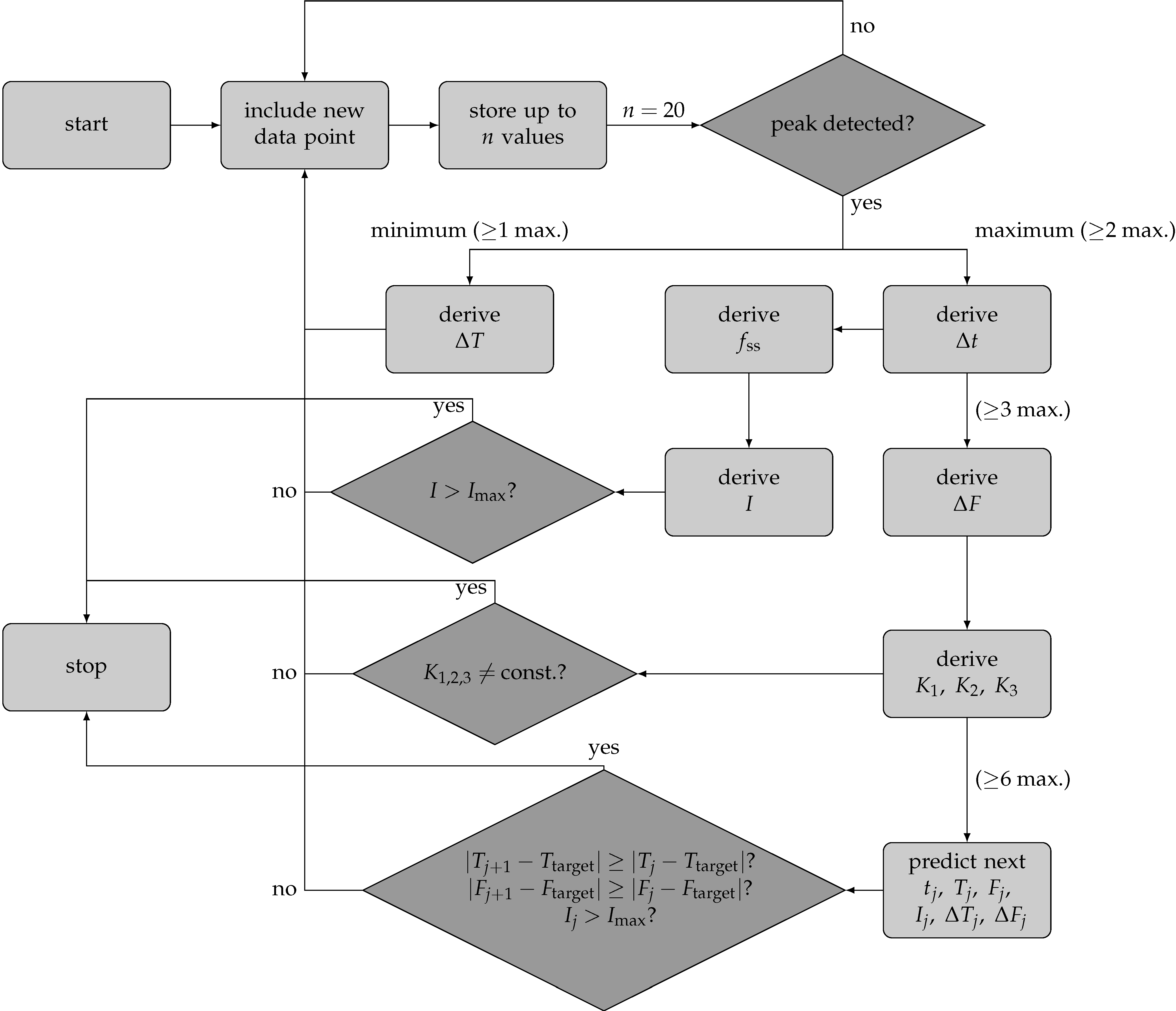
The code, shown in Figure 16, starts with recording of the first data tuple.
This tuple consists, depending on what can be measured, of the time step and a torque and/or pretension force value. In order to ensure a fast processing, a stack of 20 tuples is stored in chronological order, where the oldest is dropped for the youngest data point. After having acquired n = 20 data points, the peak detection algorithm checks for a peak inside the 20 data points. If it detects nothing, the data points show a continuous fall or raise of the data, and the algorithm waits for the next tuple to be measured. Otherwise, a maximum or minimum is detected. In order to derive the torque drop Δ T , first a maximum and then a minimum has to be detected. With two maxima being stored, the time period Δ t between them can be derived and inverted to yield the stick-slip frequency f ss . This also enables to derive the intensity I of the vibrations. After having detected three maxima, the force step Δ F can be derived (see Figure 3), because two plateaus are needed to derive the difference in magnitude. The knowledge of t, f ss , Δ t , and Δ F allow to derive the constants K 1 , K 2 , and K 3 to monitor the process. If the current intensity becomes greater than the maximum allowed intensity, or the derived constants deviate from the expected constant value, or the difference from the current to a predicted value becomes less than the threshold, the process is stopped (see Section 6.6).

6.1. Data Set for In-Situ Estimation

Only a fraction of the data that have been recorded during the tightening process needs to be processed in order to reliably identify peaks and derive further data points. Testing various alternatives, the use of n = 10 to 20 data points leads to fast and reliable results. Every time a new data tuple is introduced into the data set, the oldest will be deleted. The tuples for the torque, the force, and the time are stored in the arrays D T , T F and D t :
D T = [ T 1 , T 2 , , T n ] ,
D F = [ F 1 , F 2 , , F n ] ,
D t = [ t 1 , t 2 , , t n ] .
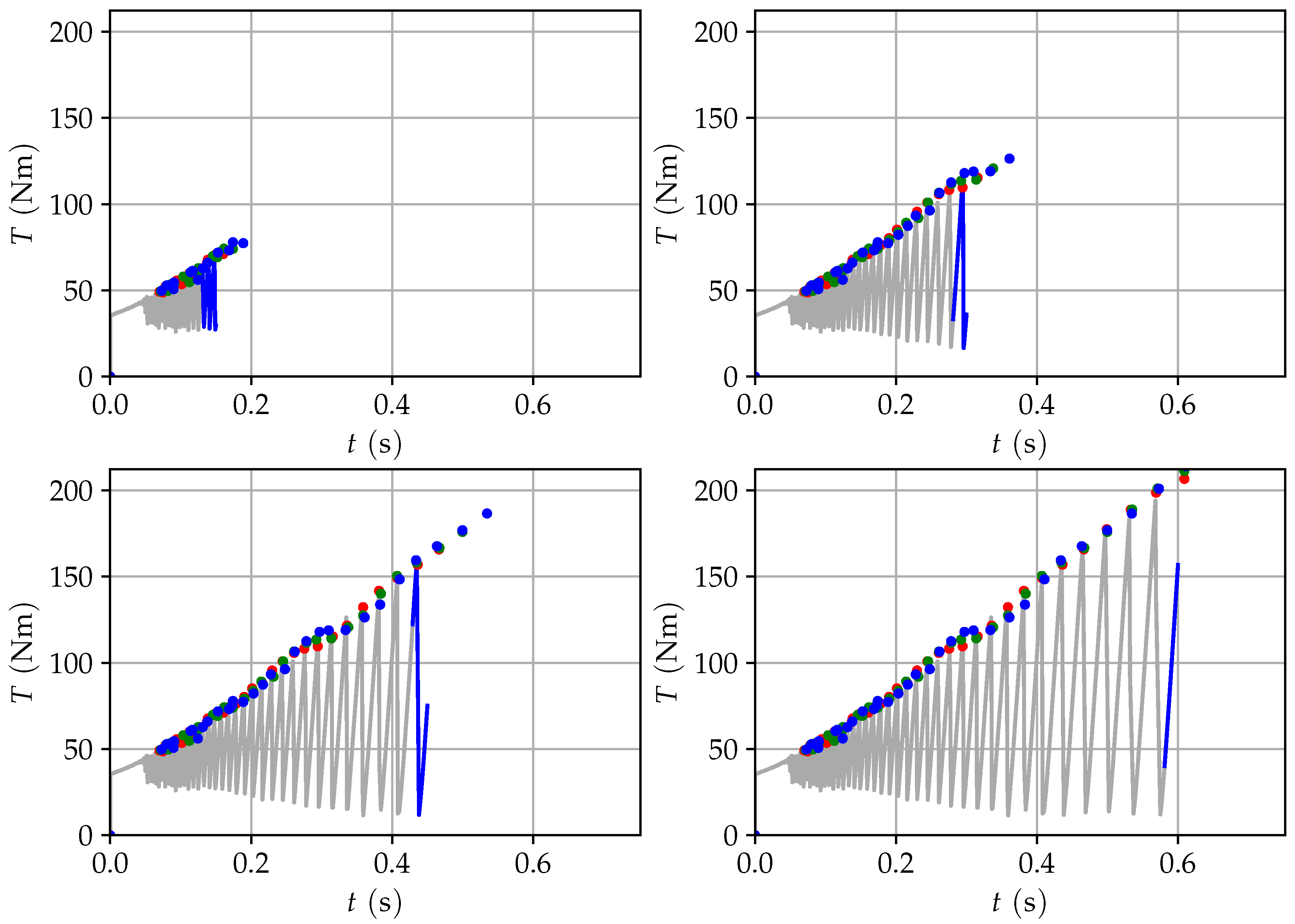
Demonstrated in Figure 17, the current data set (blue) is changing with time. The historic data (gray) do not have to be stored for this algorithm since all necessary information for further calculations lies in the list of identified peaks and the corresponding values.

6.2. Fast Peak Detection

In order to comply with the time restrictions, a fast method for the identification of peaks is used. Every time a new data point is added to the set, the peak detection algorithm is run, and the average inclination M of the set of data points D with size n is derived:
S = n Δ T i Δ t i , S = 0 M = 0 ,
M = S | S | , S 0 M [ 1 , + 1 ] .
The inclination is compared with the inclination of the previous time a data point was added. When a negative inclination ( M = 1 ) follows a positive one ( M = + 1 ), a tipping point has been passed. If the derived inclination results in M = 0 , the previous state is maintained.
The maximum value of the data points is being identified as the peak ( t max , T min ) and stored in the list of peaks. Likewise, when a positive inclination follows a negative, a minimum was passed and the data points are determined ( t min , T min ):
T max = max ( D T ) ,
t max = t ( T max ) with t D t ,
T min = min ( D T ) ,
t min = t ( T min ) with t D t .
Based on that, the prediction of the next stick-slip event can be derived. As demonstrated in Figure 17, the peaks are reliably detected. The blue curve shows the current set of data points that is used to identify the last peak.

6.3. Linear Regression of Time Variance of Stick-Slip Peaks

The stick-slip frequency is a function proportional to 1 t . Inverting the function, the time difference Δ t between the stick-slip events becomes a function proportional to time t. This relationship allows for conducting a linear regression to estimate the time difference to the next stick-slip event by utilizing the method of least squares, which aims to minimize the error E:
E = j = 0 k | p ( x j ) y j | 2 .
The returned polynomial p allows for quick evaluation, and the residuals method can be used to evaluate the quality of the fitting. The values for the linear regression are x and y:
x = [ 0 : i 1 ] ,
y = [ t i + 1 t i ] n .
The next stick-slip event is estimated to happen at Δ t n + 1 after the last occurred event:
Δ t n + 1 = p ( t n + 1 ) ,
t n + 1 = t n + Δ t n + 1 .
This point in time is useful for the prediction of the tightening torque magnitude, the tightening torque drop, the magnitude of the pretension force, and the angle of rotation. Likewise, estimations about the next and over-next events can be made. The accuracy of this prediction is investigated in Section 6.5.
Due to the fast computation capabilities, a real-time estimation of the events is possible. This is demonstrated in Figure 17 (bottom right) for three different points in time of the tightening process. The identified peaks (black) overlay the 1st estimation (red), followed by the 2nd (green) and 3rd predictions (blue). With an Intel Xeon E5-2603 v2 CPU at 1.80 GHz and 16 GB of RAM, the processing time was 0.5817 s for a tightening-time of 0.752 s.

6.4. Regression of the Peak Torques and Force Plateaus

The peak torque is estimated using the youngest five data tuples. The torque is derived using a linear regression. The prediction of the pretension force delivered best estimates using a second-order polynomial. Depending on the circumstances and the application of this algorithm, the number of data tuples and the polynomial degree can be adapted for optimal use.

6.5. Accuracy of the Stick-Slip Event Estimation

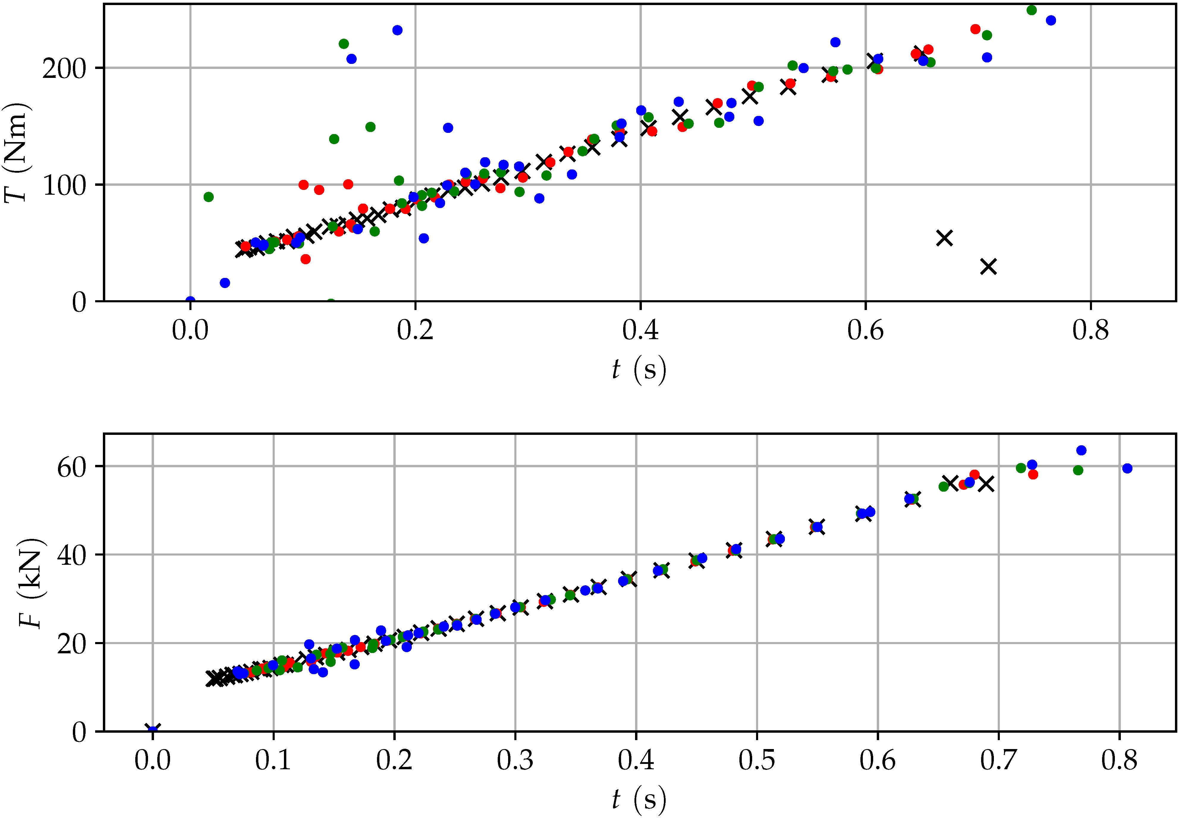
A prediction of events is only useful if it provides high accuracy (see Figure 18). During the tightening process, several stick-slip events occur until the final state is reached.
These past events cannot only be used to predict future events, but also enable an evaluation of past predictions. Based on that, the accuracy of the predictions can be estimated as follows:
δ T ^ = T i Δ T i ,
Δ F ^ = F i Δ F i ,
where δ T ^ denotes the relative peak torque difference and Δ F ^ the relative increase of the pretension force.
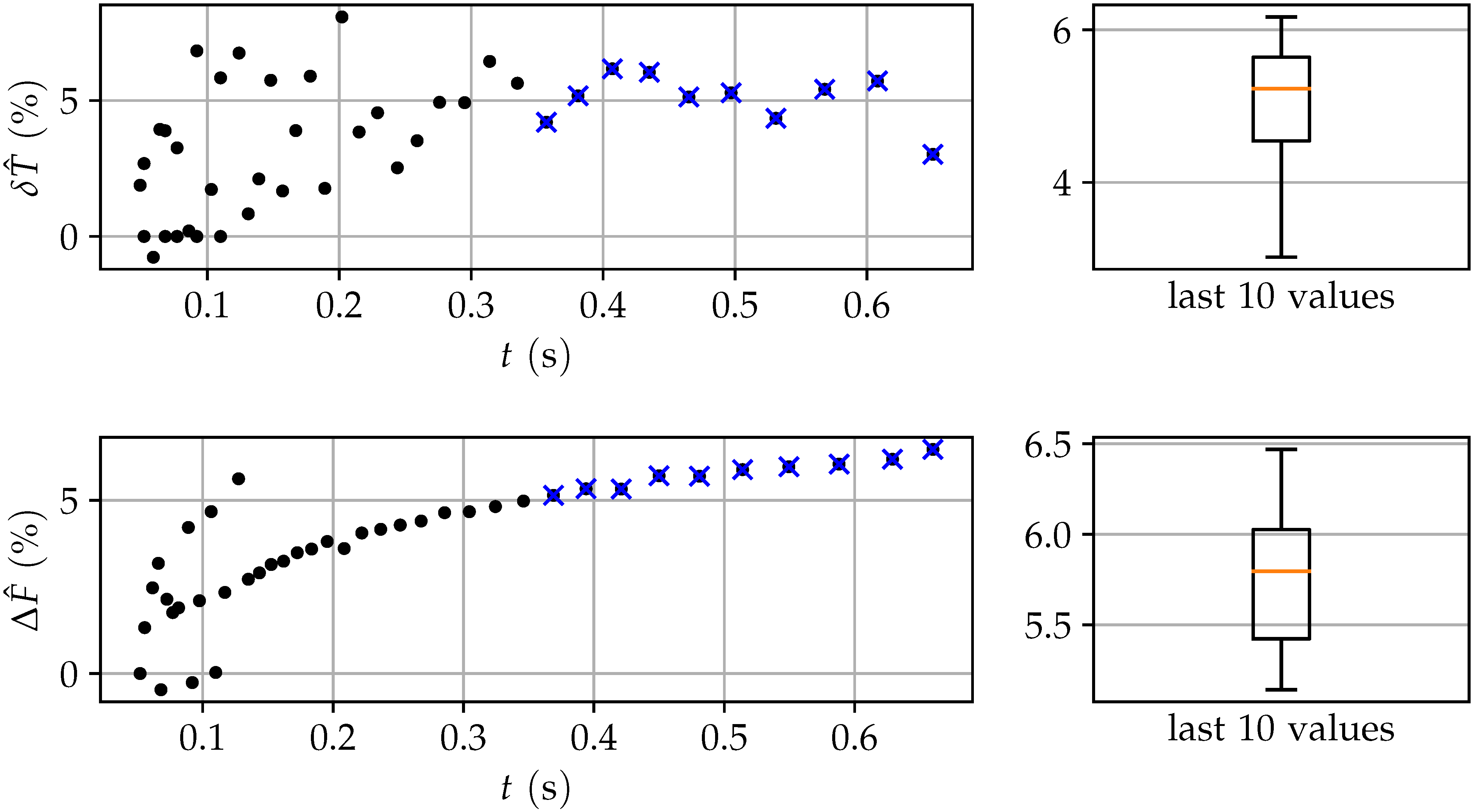
In order to evaluate the usefulness of the prediction, the system-immanent uncertainties have to be evaluated (see Figure 19).
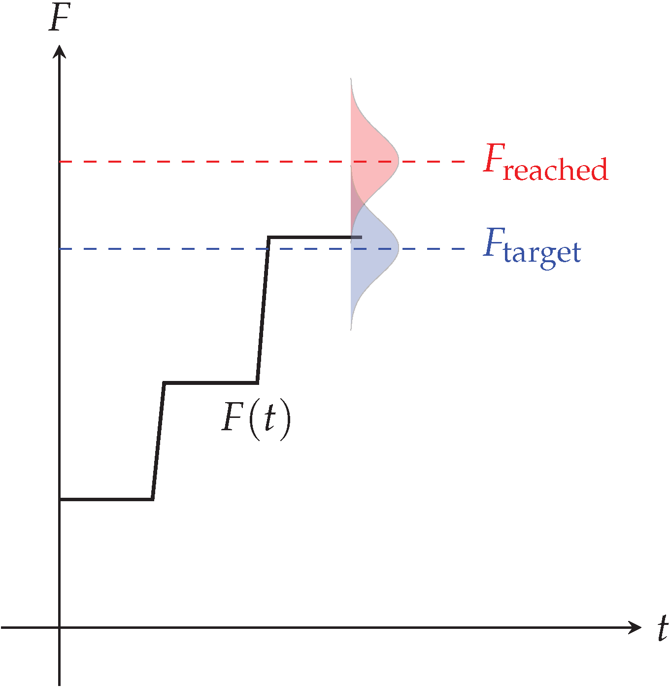
The relative peak torque difference δ T ^ yields a mean of about 5.25% over the last 10 values of the example data. Likewise, the relative increase of the pretension force Δ F ^ yields a mean of about 5.8% (see Figure 3). Common tightening methods [1,5] prescribe to surpass a minimum tightening value either in the torque or in the pretension force. This is due to the immanent uncertainty of the tightening method. The relative uncertainties of δ T ^ and Δ F ^ characterize the distribution of the final state. With the presented algorithm, it is possible to reliably reach a target value instead of overcoming a minimum (see Figure 20) and thus shift the distribution of the reached values symmetrically around F target .
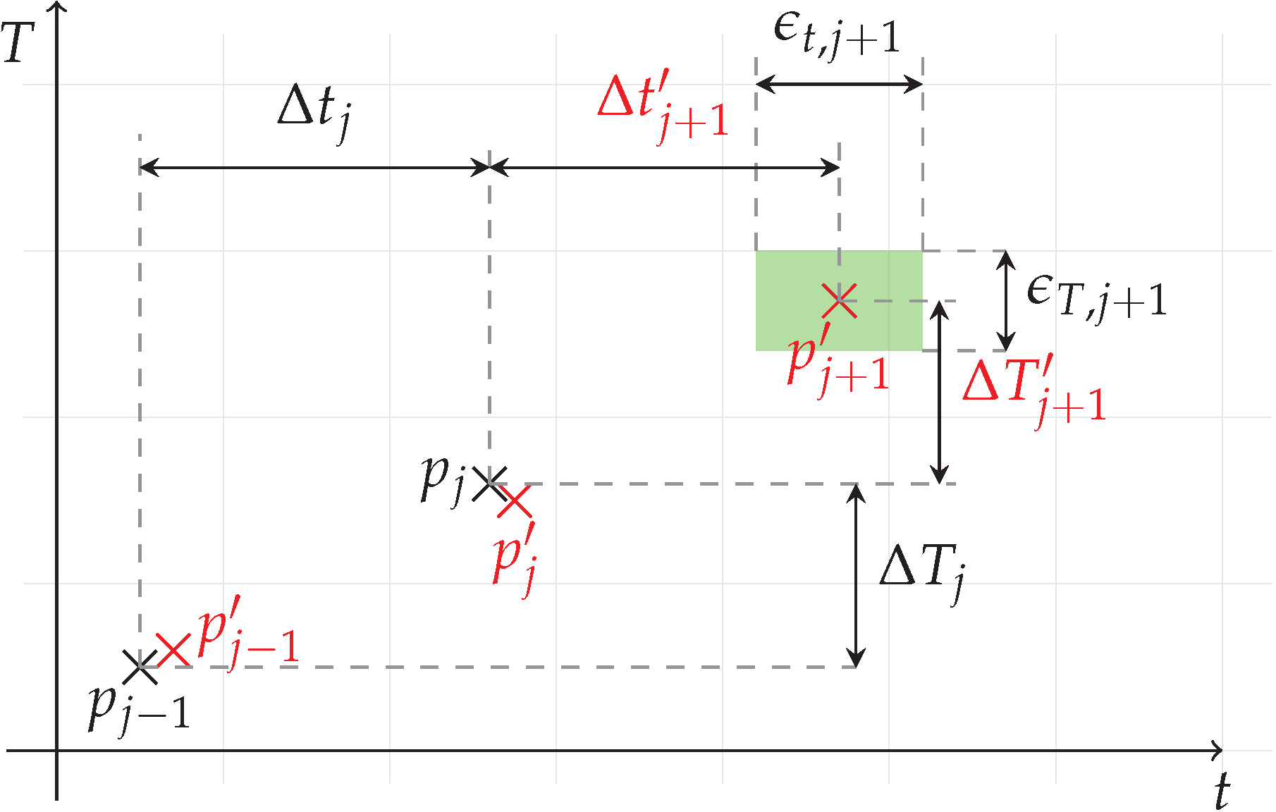
Figure 21 shows the relationship of the already detected events denoted as p j and the last prediction of these points denoted as p j in red.
Between two actual events, a time difference Δ t and a torque difference Δ T is shown (see also Figure 3). This difference is used to predict the next event, in this example denoted as p 3 . However, uncertainties in time ϵ t and in torque ϵ T , marked in green, are present. The relationship between the actual data point p j and the corresponding prediction p j can be used to derive an error:
p j = ( t j , T j , F j ) ,
ϵ ^ t = t i t i Δ t j ,
ϵ ^ T = T j T j T j ,
ϵ ^ F = F j F j F j .
Setting the difference of the predicted point time Δ t i + 1 to the actual time t in relationship to the total time of the process does not make much sense since the process is about reaching the target values of T and F, and not in a particular time. Due to the data acquisition resolution and frequency, the uncertainty of the prediction in the time domain is greater in comparison to the other two.
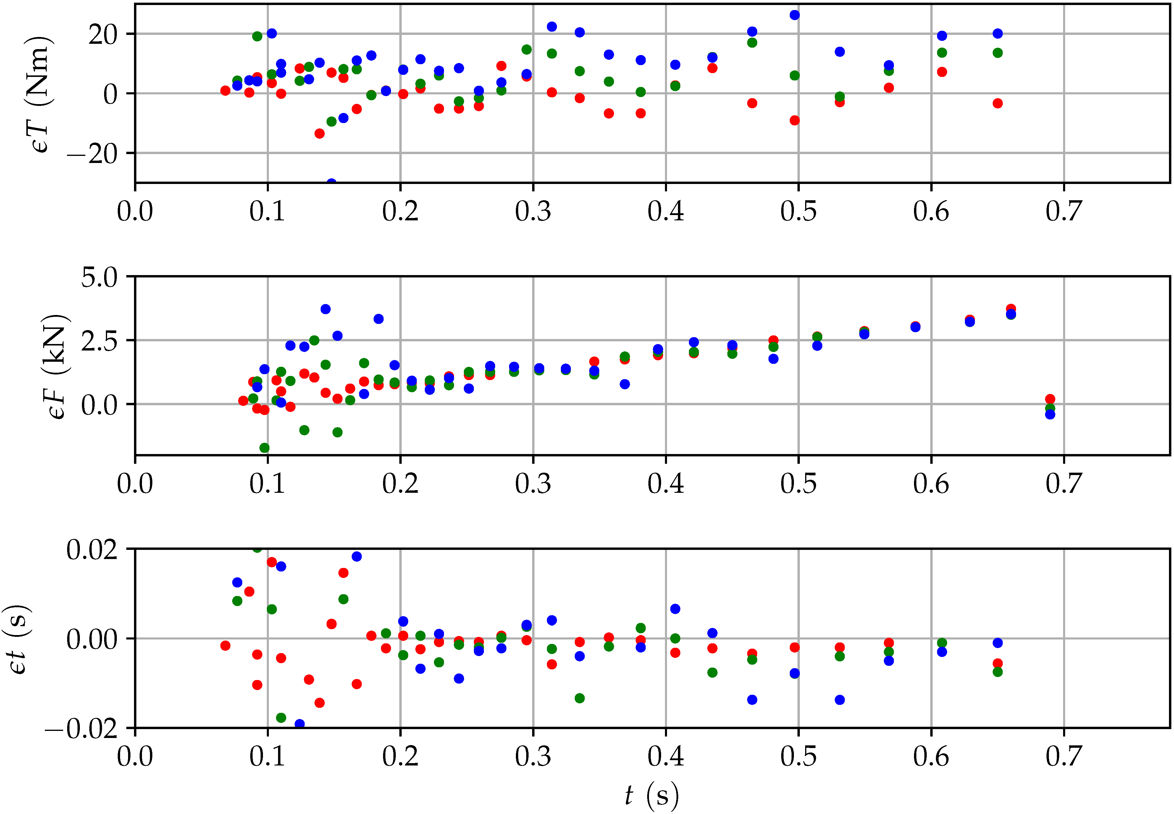
Overlaying the predicted values for the next three events on the actual data points show a very good concordance (see Figure 22).
After a short period of chaotic behavior, the error of the predicted values for time, torque, and pretension force become stable.
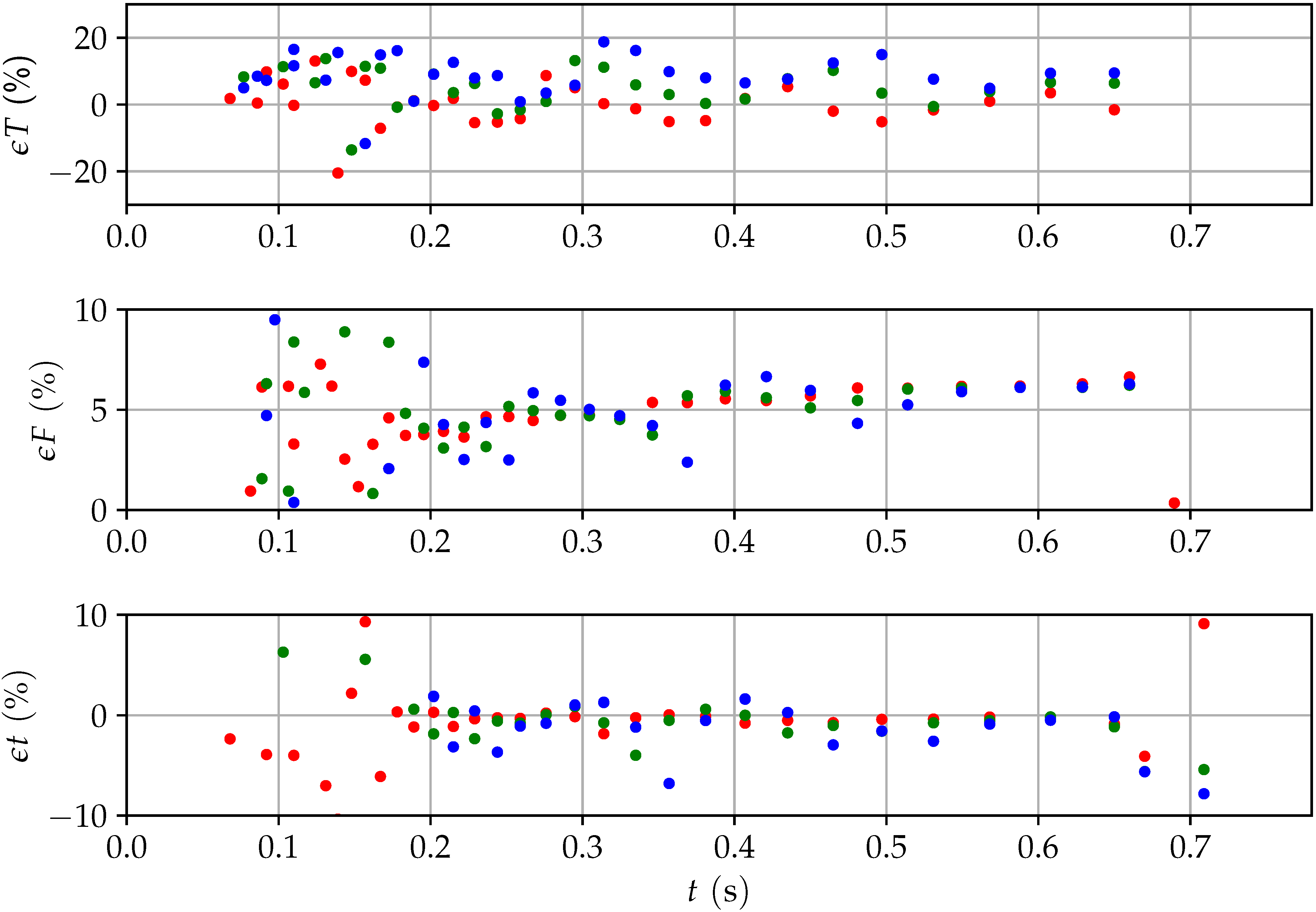
In order to set the errors in perspective, the errors are calculated in relation to the absolute values of the corresponding variable [see Figure 23 and Equations (61) to (63)].
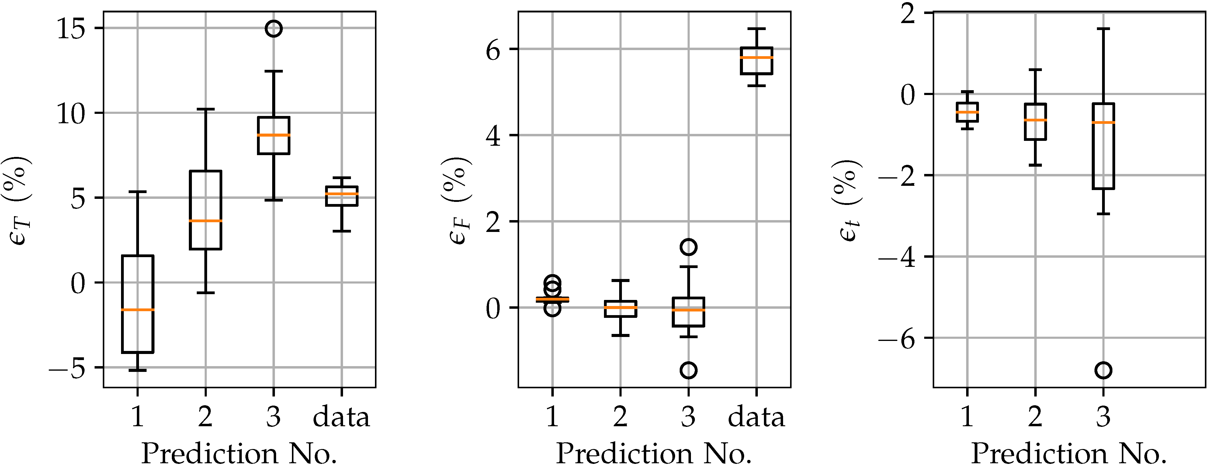
All relative errors for the first prediction show very high accuracy. The torque error in the second and third stage deviates the most in comparison to the first one. If compared with the system immanent uncertainty, see Figure 24, the second prediction still shows marginally lower uncertainty. However, the more important target value—the pretension force—can be predicted with very high precision, whereas the system immanent uncertainty is about 6% and the prediction is accurate to about 0.1% (see Figure 24).
With a 10 to 40 ms time difference between two stick-slip events, an error of about 2.5 ms might appear big. However, considering the temporal resolution of 1 ms, this is as good as it can get.

6.6. Thresholds and Safety Values

If the possibility exists to also measure the pretension force next to the torque during the tightening process, the target variable should be the pretension force since this is the primary reason to use a bolted joint. Prior to the presented algorithm, a predefined target torque T target or a target pretension force F target was defined that has to be surpassed in order to complete the tightening process. With the presented algorithm, it is possible to decide at what stage the process shall be stopped to minimize the distance of the actual torque or pretension force value and the target value. Therefore, thresholds have to be defined (see also Figure 16):
| T j + 1 T target | | T j T target | ,
| F j + 1 F target | | F j F target | .
If the distance from the next predicted value to the target value is greater than the current distance, then the process is closest to the target and will most probably defer from that goal with the next event [see Equations (64) and (65)]. Therefore, the process should be stopped now.
Friction-induced vibrations create an increased stress on the tools and the drive train. With regard to predictive maintenance, the impacts can be evaluated. The intensity is derived by taking the magnitude, the mean, and the frequency of the torque into account with j being the index for a specific stick-slip event:
T mean , j = T max , j + T min , j 2 ,
I j = Δ T j · T mean , j · f ss , j ,
I process = j = 2 n ss I j ,
I total = I process ,
I process < I max .
The total intensity of the process can be calculated using Equation (68). When the intensity exceeds the threshold I max [see Equation (70)], the process will be stopped. Similarly, the sum of all process intensities can be summed up to yield the total intensity of a machine [see Equation (69)].
Estimating the correct constants K 1 , K 2 , and K 3 [Equations (34) to (39)] in advance is difficult since they depend on the frictional contact of the joint, and that can only be accurately determined with the beginning of the tightening process. Once the constants are obtained, a deviation from the expected value can be detected and measures be conducted. The variables shall be constant during the tightening process. However, the real world application does show some degree of variance. Thus, the threshold S i is defined, which, once surpassed, will lead to a stop of the tightening process, indicating that a problem has occurred. With n ss being the number of occurred stick-slip events, and n K the number of K i values to be used to average over, the divergence of the constants can be identified as follows:
1 n K j = n ss n K 1 n ss 1 K i , j K i , n ss < S i with i = [ 1 , 2 , 3 ] .

7. Discussion

Handling frictional systems is a difficult task due to the statistical nature of its occurrence. This has led to the vague general guidelines for tightening of bolted joints. The analytical results supplement these guidelines. They show boundaries for the process values to be expected. However, they deliver boundaries and allow for an investigation of dependencies of geometric factors and process parameters without the need for computationally expensive nonlinear simulations. Some effects, like the backlash in the drive train or the gears, were not taken in consideration with the analytical model. These factors can explain an increased torque drop. Typical test rigs for bolted joints are required to withstand the high normal and torque loads during the test and simultaneously be able to record these loads with precision (see Figure 8). This leads to components which themselves have an influence on the dynamics due to the use of strain gauges, which require a certain strain (and thus relative motion) in order to change their electrical resistance. The interplay of the test rig dynamics with the joint is not considered in the current model. For the experiments, a typical combination of screw size and coating was chosen, which is common in the automobile industry. The influence of different screw and flange geometries as well as coating types has to be investigated in further research. The real-time prediction can handle the shortcomings of the analytical approach by relying on recorded data during the tightening process of a specific joint, and does not rely specifically on pre-derived analytical values. Using the prediction algorithm in contrast to the current practice of tightening until a minimum torque is exceeded, the uncertainty of the target torque or force can be reduced by about 50%. This is based on two assumptions: first, process parameters are not changed during the tightening process and, second, the goal for the process is to get as close as possible to the target values and not just exceeding a minimum value (see Figure 20). Furthermore, it opens the possibility to utilize discovered relations, like the dependency of the stick-slip frequency on the stiffness of the extension, to manipulate the vibrations during the tightening process. In combination with the highly reliable prediction of the torque and pretension force, accuracies of about 1% could be achieved.

8. Conclusions

The existence of the constants K 1 , K 2 , and K 3 gained in previous simulations [19] was proven in experiments. Instead of having to reject a joint after having experienced friction-induced vibrations, the constants can now be used to monitor the process and lead to a good end state. The analytical model provides limit values for the estimation of the pretension force F, the torque T, the torque drop Δ T , the pretension force increase Δ F , and the constants above. This makes it possible to estimate the assembly process already during the design phase of the joint. Since the analytical model only provides estimations for the process design, a real-time algorithm was presented. This algorithm can monitor the tightening process during runtime and predict an optimal time for stopping based on the actual properties of the current tightening process. In this way, the target value of the torque and force can be achieved much more accurately than it was possible with the previous tightening methods. Further improvements of the algorithm and the introduction of a mechanism which can alter the stiffness of the extension in real time could lead to a tightening process where the target values could be reached exactly, although subjected to friction-induced vibrations.

Author Contributions

Conceptualization, N.B. and A.S.; Methodology, N.B. and A.S.; Software, N.B.; Validation, N.B.; Formal Analysis, N.B.; Investigation, N.B.; Data Curation, N.B.; Writing—Original Draft Preparation, N.B. and A.S.; Visualization, N.B.; Supervision, A.S. and J.S.; Project Administration, A.S. and J.S.; Funding Acquisition, A.S. and J.S.

Funding

This work was supported by the German Research Foundation (DFG) under grant SCHL 275/13-1.

Acknowledgments

We want to thank the Hamburg University of Applied Sciences for the support during the conduction of experiments.

Conflicts of Interest

The authors declare no conflict of interest.

References

  1. VDI Guideline 2230-1. Systematic Calculation of Highly Stressed Bolted Joints—Joints with One Cylindrical Bolt; Beuth: Berlin, Germany, 2015. [Google Scholar]
  2. Johne, V. Geometrische und Kinematische Einflüsse auf die Prozesssicherheit der Industriellen Schraubmontage. Ph.D. Thesis, Technische Universität Dresden, Dresden, Germany, 2008. [Google Scholar]
  3. Nassar, S.A.; Ganeshmurthy, S.; Ranganathan, R.M.; Barber, G.C. Effect of tightening speed on the torque-tension and wear pattern in bolted connections. J. Press. Vessel Technol. 2007, 129, 426–440. [Google Scholar] [CrossRef]
  4. Deutscher Schraubenverband. Industrielle Schraubmontage: ICS Handbuch; Mönnig: Iserlohn, Germany, 2007. [Google Scholar]
  5. ISO 16047. Fasteners—Torque/clamp Force Testing; ISO: Geneva, Switzerland, 2005. [Google Scholar]
  6. Dhayagude, N.; Gao, Z.; Mrad, F. Fuzzy logic control of automated screw fastening. Robot. Comput. Integr. Manuf. 1996, 12, 235–242. [Google Scholar] [CrossRef]
  7. VDI/VDE-Gesellschaft Mess- und Automatisierungstechnik. Schraubtechnik 2008: Prozess der Schraubmontage beherrschen, VDI-Berichte 2049; VDI: Düsseldorf, Germany, 2008; Volume 2049. [Google Scholar]
  8. Croccolo, D.; de Agostinis, M.; Vincenzi, N. Failure analysis of bolted joints: Effect of friction coefficients in torque–preloading relationship. Eng. Fail. Anal. 2011, 18, 364–373. [Google Scholar] [CrossRef]
  9. Fukuoka, T.; Takaki, T. Mechanical behaviors of bolted joint during tightening using torque control. Jpn. Soc. Mech. Eng. Int. J. Ser. A Solid Mech. Mater. Eng. 1998, 41, 185–191. [Google Scholar] [CrossRef]
  10. Japing, A.; Schlattmann, J. Bolted Joints Tribology. In Encyclopedia of Lubricants and Lubrication; Springer: Berlin, Germany, 2014; pp. 183–192. [Google Scholar]
  11. Ibrahim, R.A.; Pettit, C.L. Uncertainties and dynamic problems of bolted joints and other fasteners. J. Sound Vib. 2005, 279, 857–936. [Google Scholar] [CrossRef]
  12. Scharf, P. Die Automatisierte Montage mit Schrauben: Anforderungen, alternative Fügeverfahren, Wirtschaftlichkeit, 2nd ed.; Expert: Renningen-Malmsheim, Germany, 1994; Volume 256. [Google Scholar]
  13. Croccolo, D.; de Agostinis, M.; Vincenzi, N. A contribution to the selection and calculation of screws in high duty bolted joints. Int. J. Press. Vessels Pip. 2012, 96–97, 38–48. [Google Scholar] [CrossRef]
  14. Ben-David, O.; Fineberg, J. Static friction coefficient is not a material constant. Phys. Rev. Lett. 2011, 106, 254301. [Google Scholar] [CrossRef] [PubMed]
  15. Muser, M.H. How static is static friction? Proc. Natl. Acad. Sci. USA 2008, 105, 13187–13188. [Google Scholar] [CrossRef] [PubMed] [Green Version]
  16. Hörnig, T.; Kopfer, H.W.; Friedrich, C. Torque vibrations in automatized screw assembly: Reasons, elimination and virtual testing. In Proceedings of the ASME 2013 International Mechanical Engineering Congress and Exposition, San Diego, CA, USA, 15–21 November 2013. [Google Scholar]
  17. Baramsky, N.; Seibel, A.; Schlattmann, J. Modeling of friction-induced vibrations during tightening of bolted joints. Proc. Appl. Math. Mech. 2016, 16, 259–260. [Google Scholar] [CrossRef]
  18. Japing, A.; Seibel, A.; Schlattmann, J. Modellentwicklung zur Beschreibung von Reibschwingungen bei der Schraubenmontage; Fachtagung der Gesellschaft für Tribologie (GfT): Düsseldorf, Germany, 2015; Volume 63, pp. 1–10. [Google Scholar]
  19. Baramsky, N.; Seibel, A.; Schlattmann, J. Friction-induced vibrations during tightening of bolted joints: Insights from a multi-body model. In Proceedings of the ASME 2017 International Mechanical Engineering Congress and Exposition, Tampa, FL, USA, 3–9 November 2017. [Google Scholar]
  20. Leine, R.I.; Van Campen, D.H.; De Kraker, A.; Van Den Steen, L. Stick-slip vibrations induced by alternate friction models. Nonlinear Dyn. 1998, 16, 41–54. [Google Scholar] [CrossRef]
  21. Li, Z.; Ouyang, H.; Guan, Z. Friction-induced vibration of an elastic disc and a moving slider with separation and reattachment. Nonlinear Dyn. 2017, 87, 1045–1067. [Google Scholar] [CrossRef]
  22. Lima, R.; Sampaio, R. Parametric analysis of the statistical model of the stick-slip process. J. Sound Vib. 2017, 397, 141–151. [Google Scholar] [CrossRef]
  23. Behrendt, J.; Weiss, C.; Hoffmann, N.P. A numerical study on stick–slip motion of a brake pad in steady sliding. J. Sound Vib. 2011, 330, 636–651. [Google Scholar] [CrossRef]
  24. Nassar, S.A.; El-Khiamy, H.; Barber, G.C.; Zou, Q.; Sun, T.S. An experimental study of bearing and thread friction in fasteners. J. Tribol. 2005, 127, 263–272. [Google Scholar] [CrossRef]
  25. Nassar, S.A.; Sun, T.S. Surface roughness effect on the torque-tension relationship in threaded fasteners. Proc. Inst. Mech. Eng. Part J J. Eng. Tribol. 2007, 221, 95–103. [Google Scholar] [CrossRef]
  26. Stephen, J.; Marshall, M.; Lewis, R. An investigation into contact pressure distribution in bolted joints. Proc. Inst. Mech. Eng. Part C J. Mech. Eng. Sci. 2014, 228, 3405–3418. [Google Scholar] [CrossRef]
  27. Marshall, M.B.; Lewis, R.; Dwyer-Joyce, R.S. Characterisation of contact pressure distribution in bolted joints. Strain 2006, 42, 31–43. [Google Scholar] [CrossRef]
  28. Gong, H.; Liu, J.; Ding, X. Calculation of the effective bearing contact radius for precision tightening of bolted joints. Adv. Mech. Eng. 2016, 8, 1–8. [Google Scholar] [CrossRef]
  29. Kellermann, R.; Klein, H.C. Berücksichtigung des Reibungszustandes bei der Bemessung hochwertiger Schraubenverbindungen. Konstruktion 1956, 4, 236–244. [Google Scholar]
  30. Hörnig, T.; Födisch, F.; Friedrich, C.; Johne, V.; Füssel, U. Stick-Slip-Ereignisse bei der Schraubmontage: Analyse—Einflüsse—Vermeidung; University of Siegen: Siegen, Germany, 2012. [Google Scholar]
  31. Sadd, M.H. Elasticity: Theory, Applications, and Numerics, 2nd ed.; Elsevier: Amsterdam, The Netherlands, 2009. [Google Scholar]
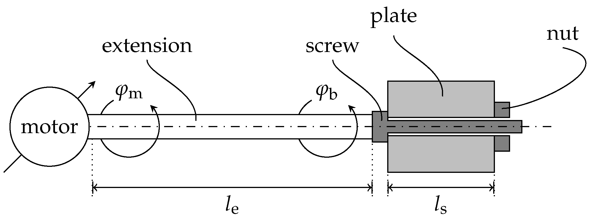
Figure 1. The tightening rig is reduced to an ideal linear motor, an elastic extension, and a stiff screw, which is bolted into a plate to analytically describe the stick-slip constraints.
Vibration 01 00021 g001
Figure 2. Demonstration of the relationship between the motor angle φ m and different states of the bearing angle φ b during stick and slip.
Vibration 01 00021 g002
Figure 3. Definition of process metrics: Δ T j : torque drop from maximum to successive minimum; δ T j : torque difference of two successive maxima; Δ t : time difference of two successive maxima; Δ F j : increment of two successive pretension force plateaus; Δ t j * : corresponding time difference of the plateaus. The suffixes j defines the affiliation to a specific stick-slip event. The suffixes ‘max’ and ‘min’ define boundaries for a specific value.
Vibration 01 00021 g003
Figure 4. Demonstration of the difference of the stick-slip frequency f ss between fast and slow angular velocities over time (left) and relative to the progress of the tightening process (right).
Vibration 01 00021 g004
Figure 5. Utilizing entry and exit windows to control the tightening process. Friction-induced vibrations hinder the use of the windows due to their significant variance in magnitude.
Vibration 01 00021 g005
Figure 6. Dependency of geometric and frictional parameters on the factors γ stick and γ slip . The used parameter values are listed in the text.
Vibration 01 00021 g006
Figure 7. Natural frequency f n of the extension with G = 81 GPa and ρ = 7900 kg m 3 over length l e .
Vibration 01 00021 g007
Figure 8. Schematic of the tightening test rig with the drive train and extension tightening the screw against clamped parts, which include sensors to measure friction torques and the pretension force.
Vibration 01 00021 g008
Figure 9. The screw is tightened using a nut and an extension (left). Both only apply torque and no normal load. The nut is held in place by an adapter (right), which allows for adjusting the clamping distance with intermediate parts.
Vibration 01 00021 g009
Figure 10. Torque (top) and pretension force (bottom) over time with identified maximum and minimum peaks of the applied torque and the analytically derived maximum and minimum values in solid lines. The pretension force F is presented with the identified plateaus and the maximum and minimum analytical results of the step-like progress.
Vibration 01 00021 g010
Figure 11. Analytically derived angles over time; φ m : angle of the motor at the beginning of the drive train; φ b , min : minimum angle of the bearing of the screw due to stiction; φ b , max : maximum angle of the bearing due to slip; Δ φ b : magnitude of the angle of the bearing that is rotated during the switch from stiction to slip.
Vibration 01 00021 g011
Figure 12. Phosphated screws (left) and cathodic dip coated metal sheets (right) with drill holes.
Vibration 01 00021 g012
Figure 13. Frequency f ss over time (top) and constant K 1 over time (bottom) with analytically derived boundaries.
Vibration 01 00021 g013
Figure 14. Increase of the pretension force Δ F per slip event over time with the analytically derived maximum and minimum values (top). The approximated lines for a relief of just 50% of the energy is shown in dashed lines. The constant K 2 demonstrates the increase of pretension force per time interval of a stick-slip event (bottom), and is characteristic for a joint type.
Vibration 01 00021 g014
Figure 15. Torque drop Δ T per slip event over time with the analytically derived maximum and minimum values (top). The approximated lines for a relief of just 50% of the energy difference between the stiction and sliding status is shown in dashed lines. The constant K 3 demonstrates the torque drop per time (bottom), and is characteristic for a joint type.
Vibration 01 00021 g015
Figure 16. Structure of the real-time code constantly evaluating the stick-slip process.
Vibration 01 00021 g016
Figure 17. Sequence of four different points in time of the prediction of the next stick-slip event in time and magnitude (red: 1st; green: 2nd; blue: 3rd prediction).
Vibration 01 00021 g017
Figure 18. Predictions for torque and pretension force (red: 1st; green: 2nd; blue: 3rd prediction).
Vibration 01 00021 g018
Figure 19. Relative uncertainties of the detected peaks for the torque T ^ and the plateaus of the pretension force F ^ due to the stick-slip phenomenon during tightening.
Vibration 01 00021 g019
Figure 20. Qualitative statistical distribution of the pretension force end state F reached with conventional process control, which will always be above the minimum F target . The blue distribution shows the reached force around F target due to the new process control based on the predictions.
Vibration 01 00021 g020
Figure 21. Prediction of the next stick-slip event (denoted with ’) with corresponding actual values and error intervals at the example of T.
Vibration 01 00021 g021
Figure 22. Absolute errors for torque, pretension force, and time over time for the predicted values (red: 1st; green: 2nd; blue: 3rd prediction).
Vibration 01 00021 g022
Figure 23. Relative errors for torque, pretension force, and time over time for the predicted values (red: 1st; green: 2nd; blue: 3rd prediction).
Vibration 01 00021 g023
Figure 24. Error bars for the relative errors of the torque ϵ ^ T , force ϵ ^ F , and time ϵ ^ t in comparison to the system immanent relative uncertainty.
Vibration 01 00021 g024