Article

A Robust Methodology for the Reconstruction of the Vertical Pedestrian-Induced Load from the Registered Body Motion

by
Katrien Van Nimmen
1,2,*,
Guoping Zhao
3,
André Seyfarth
3 and
Peter Van den Broeck
2
1
Department of Civil Engineering, Structural Mechanics, KU Leuven, B-3001 Leuven, Belgium
2
Department of Civil Engineering, Technology Cluster Construction, Structural Mechanics, KU Leuven, B-9000 Ghent, Belgium
3
Lauflabor Locomotion Laboratory, Institute of Sport Science, Centre for Cognitive Science Technische Universität Darmstadt, Magdalenenstr. 27, D-64289 Darmstadt, Germany
*
Author to whom correspondence should be addressed.
Vibration 2018, 1(2), 250-268; https://doi.org/10.3390/vibration1020018
Submission received: 4 July 2018 / Revised: 29 October 2018 / Accepted: 31 October 2018 / Published: 7 November 2018
(This article belongs to the Special Issue Vibration Serviceability of Civil Engineering Structures)

Abstract

:
This paper proposes a methodology to reconstruct the vertical GRFs from the registered body motion that is reasonably robust against measurement noise. The vertical GRFs are reconstructed from the experimentally identified time-variant pacing rate and a generalised single-step load model available in the literature. The proposed methodology only requires accurately capturing the body motion within the frequency range 1–10 Hz and does not rely on the exact magnitude of the registered signal. The methodology can therefore also be applied when low-cost sensors are used and to minimize the impact of soft-tissue artefacts. In addition, the proposed procedure can be applied regardless of the position of the sensor on the human body, as long as the recorded body motion allows for identifying the time of a nominally identical event in successive walking cycles. The methodology is illustrated by a numerical example and applied to an experimental dataset where the ground reaction forces and the body motion were registered simultaneously. The results show that the proposed methodology allows for arriving at a good estimate of the vertical ground reaction forces. When the impact of soft-tissue artefacts is low, a comparable estimate can be obtained using Newton’s second law of motion.

1. Introduction

Footbridges are often conceived as slender and lightweight structures and are, by consequence, sensitive to human excitation [1]. Currently, the response of these structures to human-induced loading is predicted based on equivalent load models, up-scaled from single-person force measurements [2,3]. Although the dynamic performance under high crowd densities is often imperative for the design, these loading conditions have virtually never been verified [4]. Concerns about these load models are strengthened by the fact that recent studies indicate the significant impact of human–structure interaction (HSI) phenomena [5,6,7,8,9]. However, large-scale experimental evidence corroborating these results is absent.
The further development and calibration of pedestrian excitation models requires in-field observations for they are the only way to obtain detailed and accurate information on representative operational loading data [4,10]. As direct force measurements are in this case practically infeasible, indirect force measurements, where the input is reconstructed from registered body motion, constitute an interesting alternative. Promising results have been obtained for the reconstruction of the ground reaction forces (GRFs) induced by walking, bobbing and jumping, generally using visual marker data [8,11,12,13] and in some cases using inertial sensors [14,15,16,17,18,19]. In [12], Racić et al. apply Newton’s second law of motion and the vertical accelerations at the centre of mass (CoM) of 15 body segments, in order to reconstruct human bouncing and jumping forces. The vertical accelerations were obtained by differentiating the tracked marker displacements twice with respect to time. A good match is obtained in the frequency content between the measured and the reconstructed vertical GRFs. In a similar way, Carroll et al. [13] reproduced the lateral GRFs induced by walking from 31 active markers and used this to analyse the pedestrian’s balance when walking on a laterally oscillating deck. In [20], Dang et al. used up to 27 markers to experimentally characterize the walking locomotion on rigid surfaces. For jumping and bobbing, McDonald et al. [11] show that the tracked marker motion of the C7th vertebrae (C7) at the base of the neck is a good approximation of the motion of the body center of mass (BCoM). They show that using the nominal body mass with the motion of C7 in Newton’s second law allows for arriving at a good approximation of the corresponding induced GRFs. In addition, these studies use the tracked marker data to quantify the variability in the induced GRFs. Deriving GRFs from kinematic data is a challenge as the position data need to be differentiated twice to obtain the underlying forces. Additionally, the marker positions are not fixed with respect to the skeleton (e.g., skin and cloths movements) and the body segments are not rigid [21]. As a consequence, the derived force data from marker positions do not accurately represent the accelerations of the body parts.
Although marker-based technologies are the golden standard for laboratory applications, they are practically infeasible for application in the field involving a large number of participants because of marker occlusion and the limitations of the tracking devices in terms of distance. An interesting alternative is the use of individually-adopted sensor technologies, such as inertial sensors [14,15,16,17,18,19]. In [15], a laboratory setup involved a single pedestrian whereby the vertical acceleration levels close to the BCoM are measured simultaneously with the induced GRFs. The tests involved a rigid laboratory floor and a flexible laboratory footbridge. Toso et al. [15] then used the spectral acceleration amplitudes of the first three harmonics at the waist level and the corresponding amplitudes of the first three harmonics of the vertical GRF as inputs to fit a biomechanical model for pedestrian-structure interaction. The waist level is close to the L5th vertebrae (L5) and thereby assumed to be close to the BCoM. Based on single-person tests on rigid surface, Shahabpoor et al. [22] determined the optimal inertial sensor location and combination to reconstruct the triaxial GRFs from the measured acceleration levels of different body segments. In their work, a linear model is proposed that can be trained for an individual, to estimate the GRFs with a high level of accuracy from the acceleration levels registered at C7, L5 and one of the thighs. Bocian et al. [16] showed that using the nominal body mass with the motion of C7 in Newton’s second law yields an absolute error in the amplitude of the component of force at the pacing frequency of less than 15 percent at a 90 percent confidence level. Furthermore, Bocian et al. [16] use the data collected by wireless altitude and heading reference systems to estimate the spatial location of application of the pedestrian forces. In [17], Brownjohn et al. use the data collected by wireless inertial units at C7 and Newton’s second law to arrive at a good estimate of the GRFs induced by jumping. In more recent work, Brownjohn et al. [19] propose a linear combination of body accelerations measured at the lower back and sternum positions to reproduce the medio-lateral walking GRFs. In [14,18], wireless inertial sensor technologies are used at a single location on the human body, close to the BCoM, to track the walking behaviour of pedestrians on a real footbridge. The data is used to characterize the walking load and to analyse the level of synchronization among the individuals. In addition, Bocian et al. [18] use this technique to analyse the synchronization between the structural vibrations and the walking behaviour of the pedestrians.
The (wireless, low-cost) sensors used to simultaneously track the motion of multiple pedestrians are generally more sensitive to low-frequency drifts and are characterized by a lower sensitivity and sampling rate than the state-of-the-art (maker-based) technologies usually applied in laboratory conditions. Furthermore, as in the field sensors are often applied on top of one or more layers of clothing, a larger impact of soft-tissue artefacts [12,21] is to be expected. The use of this data for the characterization of the human-induced load is therefore not straightforward and requires careful attention.
When the GRFs are reconstructed using Newton’s second law of motion, the accuracy of the reproduction is directly related to the accuracy of the sensor that is used to register the body motion. Additional sources for the error in the reconstructed GRFs are the assumption that a single point on the body surface has the same kinematics as the BCoM and soft-tissue artefacts [11]. An alternative methodology is presented in [14], where the GRFs are reconstructed from the time-variant pacing rate, identified from the motion of a point on the body with kinematics that approximates those of the BCoM, and a generalised single-step load model available in the literature [23,24]. This methodology is only applicable for certain points on the human body. Furthermore, although the accuracy of the estimate of the GRFs does not depend on the exact magnitude of the registered signal, it depends on the accuracy of the identification of the time-variant pacing rate. As in [14], the time-variant pacing rate is identified from the time between successive peaks in the registered body motion, and the accuracy of the reconstruction requires a high sampling rate and is affected by soft-tissue artefacts.
In view of in-field applications, the present study introduces a methodology to reconstruct the vertical GRFs from the registered body motion, which is reasonably robust against measurement noise arising from soft-tissue artefacts and the application of low-cost sensor technologies. To this end, the methodology is developed that uses the motion registered at a single location on the human body and allows the body kinematics to be collected at a relatively low sampling rate (e.g., 25 Hz). The key element is the procedure proposed to identify the time-variant pacing rate from the registered body motion, which does not rely on the exact magnitude of the registered signal nor the position of the sensor on the human body. Similar to the approach presented in [14], the vertical GRFs are then reconstructed from the experimentally identified time-variant pacing rate and a generalised single-step load model available in the literature [23,24]. Although small variations in force amplitude or contact time are in this way not accounted for, this simplification is considered acceptable as the structural response is primarily sensitive to variations of the pacing rate (and the weight) of the persons, as also observed by [14,25].
The procedures used in the experimental work are approved by the ethical committee of the involved university hospitals (KU Leuven and TU Darmstadt) and each subject gave written informed consent prior to participation.
The outline of this paper is as follows. First, the experimental dataset is described (Section 2). Second, an initial estimate of the GRFs is made based on Newton’s second law of motion (Section 3). Third, an innovative approach is introduced to estimate the GRFs from the registered body motion (Section 4). This approach is first verified numerically and subsequently applied to the experimental dataset. Finally, the conclusions are formulated.

2. Experimental Data

The data used in this study involves treadmill data and is collected in the Movement and posture Analysis Laboratory Leuven (MALL) at the Department of Kinesiology of KU Leuven [26] and the Lauflabor Locomotion Laboratory of the Institute of Sport Science at TU Darmstadt. The main advantage of the treadmill technology is that it allows for the identification of stride-to-stride variations [27].
The experimental study at the MALL involved two experienced treadmill users (participants 1 and 2, in Table 1). The GRFs were registered by an instrumented split-belt treadmill (Forcelink) with a sampling rate of 1 kHz. Six walking speeds were considered for participant 1, and three walking speeds for participant 2 (see Table 1). For each walking speed, a measurement time of 2 min was considered which allowed for the registration of approximately 200 steps for each trial. For each trial, a period of at least 30 s was provided to allow the participant to adapt his walking behaviour to the selected treadmill speed. In addition to the GRFs, a 3D inertial motion tracking system was used to register the accelerations of the body segments. To do so, multiple wireless inertial units were securely fixed onto the participant with specially designed click-in full body straps. In [14], a total of six sensors was used. The present study only uses the data collected by the sensor placed as close as possible to the BCoM located at the level of the 5th lumbar vertebrae (L5) using the pelvis belt. The main reason for doing this is because the number of sensors attached to each person is to be limited such that the methodology is also practically feasible for large-scale experiments involving a large number of persons. In addition, in [14], it is shown that, for the involved six sensor positions, including L5 and T6 (sixth thoracic vertebrae), the strongest correlation exists between the GRFs and the accelerations of the BCoM. It is noted, however, that, in [16], an even better correlation with the GRFs is found when using the C7 accelerations, in particular for slow walking speeds. The sampling frequency of the inertial units was set to 60 Hz, as recommended by the manufacturer for a configuration of six sensors. The GRFs and inertial sensor data are synchronised through the use of a trigger signal.
The experimental study at the Institute of Sport Science involved two participants (participants 3 and 4, in Table 1). The GRFs were registered by an instrumented treadmill (HEF Tecmachine, Kistler force sensors, Winterthur, Switzerland) with a sampling rate of 240 Hz. Two walking speeds were considered for participant 3, and three walking speeds for participant 4 (see Table 1). In order to estimate the CoM movement, a marker was placed on the back of the pelvis (sacrum). A motion capture system (Qualisys, Gothenburg, Sweden) was used to record the marker position at a frequency of 500 Hz. The measurement time of each speed condition was 3 min.
To minimise the influence of instrumental noise and moving parts of the treadmill [28] and measurement noise on the body kinematics, a cut-off frequency of 12 Hz is applied to the GRFs and body motion data using a fifth order Chebyshev type I lowpass filter. In this way, the low-frequency content (0–10 Hz) that is relevant for the vibration serviceability of footbridges [1] is retained. To allow for a sufficient high resolution in the time-domain analysis of the subsequent sections, the signals are resampled at a sampling rate of 1000 Hz. Section 4 will further analyse the required resolution in time-domain.
Given the focus of the paper, only the vertical component of the GRFs and the registered body motion are retained. For each trial, the corresponding mean step frequency f ¯ s is identified as the dominant contribution in the Power Spectral Density (PSD) of the registered GRFs (or motion of the human body) in the relevant frequency range [1.0–2.5] Hz (see also Table 2). For the present application, the PSD is calculated using Welch’s method with 50% overlap and a Gaussian window with a length of 20 s [29]. These window properties can be chosen based on engineering judgement: the sole purpose of the PSD is to obtain an average amplitude spectrum from which a rough estimate of the mean step frequency can be derived (see also Section 4.1.2 and Section 4.3).

3. Initial Approximation: Newton’s Second Law

Theoretically, the GRFs during locomotion can be calculated from Newton’s second law that states that the external force acting upon a body equals the product of the body’s mass m concentrated at its BCoM and the corresponding acceleration u ¨ COM . For the vertical GRFs acting on the human body ( p GRF ), it follows:
p GRF ( t ) = m u ¨ COM ( t ) + g ,
where g represents gravity and G = m g [N] the weight of the body. Considering the human body as a system with n s segments yields:
p GRF ( t ) = s = 1 n s m s u ¨ s ( t ) + g ,
where m s is the mass attributed to segment s, u ¨ s represents the vertical acceleration of the BCoM of the s th body segment and m = s = 1 n s m s .
In inverse dynamic analyses, the GRFs are quantified based on kinematic measurements in combination with the anthropometry of the human body, i.e., the physical properties of the body segments [30,31]. The latter is in this case restricted to the body segment’s inertial parameters: its mass and BCoM. The kinematic measurements are performed using technologically advanced tools for analysing the human motion, for example the optical marker-based technology of Vicon [32] and CODA [33]. These inverse methods are generally computationally expensive and the accuracy of the identified forces strongly depends on the accuracy of both the applied biomechanical model and the available experimental data, in particular the measured limb motions [30].
As motivated in the previous sections, only the vertical acceleration levels registered at the BCoM ( u ¨ COM ) are of interest. For participants 3 and 4, these BCoM accelerations are obtained as the second derivative of the vertical marker data. For participants 1 and 2, inertial sensors were used. Inertial sensors generally register acceleration levels in the device’s local coordinate system. In the present study, the applied devices also register their orientation. This information is applied to convert the local acceleration data to a global reference coordinate system [34], i.e., coordinate system of the treadmill. Another issue is that the BCoM is normally located within the person’s trunk; hence, it is not directly accessible [11]. Furthermore, the location of the BCoM is changing throughout the walking cycle. Assuming that for walking the changes in the BCoM are small and using the accelerations measured at a location on the body as close as possible to the BCoM ( u ¨ COM ( t ) ), i.e., located at the level of the 5th lumbar vertebrae (Section 2), a first approximation of the measured GRFs is found using u ¨ COM ( t ) and the nominal body mass m according to Equation (1).
The results obtained for participant 1 are used as the leading example throughout the remainder of this study. In addition, a summary of the results for all trials and all participants is presented and discussed.
The comparison between the measured and reconstructed GRFs for participant 1 for a walking speed of 5.5 km/h is presented in Figure 1. The corresponding amplitude spectrum is presented in Figure 2. The coefficient of determination R 2 [11,35] is used to quantify the fit between the original and the reconstructed GRFs in both the time domain ( R t 2 ) and the frequency domain, using the amplitude spectrum ( R f 2 ). Figure 1 illustrates that although the measured ( p ˜ GRF ) and the reconstructed ( p GRF ) GRFs appear highly correlated, the amplitudes of the reconstructed GRFs significantly exceed the ones of the measured GRFs. This difference is also clearly reflected in the corresponding amplitude spectrum (Figure 2). For the test involving a walking speed of 5.5 km/h, an R 2 coefficient of 0.863 and 0.889 is obtained for the fit in time domain and amplitude spectrum, respectively. Similar observations and R 2 coefficients are obtained for the other walking speeds (Table 2) and the full experimental dataset (Figure 3).
The main sources for the error in the reconstructed GRFs are the assumption that a single point on the body surface has the same kinematics as the BCoM and soft-tissue artefacts [11]. To reduce this error, a magnitude scaling α eff can be applied to the body mass, resulting in an effective body mass m eff = α eff m [36]. The optimal scale factor α eff is dependent on the participant and the walking speed. In the work of Silva et al. [37,38], this scale factor α eff is found to vary between 42% and 92% and to decrease for an increasing walking speed. For the present application, the average scaling factor ( α ¯ eff ) is estimated as the linear magnitude scaling factor that minimises the difference between the PSD of the reconstructed GRFs and the PSD of the measured GRFs. Table 2 shows that, for participant 1, an average fraction of 76% is found. By considering the corresponding effective body mass in Equation (1), the R 2 coefficient for the test involving a walking speed of 5.5 km/h increases to 0.962 and 0.982 for the fit in time domain and amplitude spectrum, respectively. Table 2 shows that similar results are obtained for the entire range of the considered walking speeds.
This section shows that a fair approximation of the GRFs is obtained using the acceleration levels registered at the BCoM and the effective body mass in Equation (1). However, this procedure has two drawbacks. First, the reconstruction of GRFs from joint kinematics is in particular challenged by the impact dynamics of soft tissue. The optimal scale factor α eff depends on the body composition of soft (e.g., muscles, connective tissue, fat) and rigid (bones) parts, but also on the joint configuration (bent vs. extended joints [36]) and the muscle activity [21]. The fraction α eff m thus depends on the walking speed as well as on the individual (inter-person variability). Second, this procedure is only applicable when the acceleration levels are collected on a location on the human body close to the BCoM. In case the applied inertial sensors only register the acceleration levels in the device’s local coordinate system, additional estimation errors may result from orientation errors or changes.

4. New Approach: Combining the Experimentally Identified Time-Variant Pacing Rate with a Single-Step Load Model

In this section, it is analysed how accurately the GRFs can be reconstructed using the identified time-variant pacing rate together with a generalized single-step load model available in the literature.
First, a numerical analysis is performed (Section 4.1) to investigate how the time-variant pacing can be identified with a high level of accuracy in the absence of measurement noise (Section 4.1.1). In addition, the impact of integrating a lowpass filter with a cut-off frequency at 1.5 × f ¯ s or 2.5 × f ¯ s in the preprocessing of the input signals (Section 4.1.2) and the applied single-step load model (Section 4.1.3) is analysed. Second, the proposed methodology is applied on the experimental dataset described in Section 2 (Section 4.2). The methodology is schematically presented and summarized in Section 4.3.

4.1. Numerical Investigations

The numerical investigations in this section are based on the walking load as numerically simulated using single-step load models available in the literature [23,24]. The intra-person variability in the walking load is simulated by considering a time-variant pacing rate, or, equivalently, a time-variant pacing period. The variability in step frequency is set to match the variability as identified for the previously described treadmill trials (see Section 3 and [14]). For these trials, the step-by-step pacing rate is characterized by an average standard deviation of 0.04 Hz. As for treadmill walking, the walking speed is fixed, and it can be assumed that the corresponding intra-person variability is low in comparison to the one for in-field applications. Analyses show, however, that, when the degree of intra-person variability is reasonably increased, e.g., up to two or three times the standard deviation as observed for treadmill trials, similar results are obtained as the ones presented in the following paragraphs.

4.1.1. Identification of the Time-Variant Pacing Rate

The time-variant pacing rate, or, more specifically, the time between two successive steps can be identified as the time between the nominally identical events of successive cycles [39]. When the individual foot traces of the GRFs are available, the time-variant pacing rate can be easily determined by identifying the time corresponding to the first non-zero value, or onset, for each step. This procedure is no longer applicable when not the feet’s individual GRFs, but the body motion is used as input as the human body is not at rest between two steps. In [14], the time-variant pacing rate was identified based on the identification of the time between the peaks observed during the double-stance phase (double-stance peak, Figure 4b). The timing of this peak is influenced by the timing of the two overlapping steps. Alternatively, this study proposes to identify the time between the dips in the foot traces (single-step dip, Figure 4b), or the corresponding event in the body motion. These dips occur in a time frame where only a single foot is in contact with the ground.
The proposed methodology is illustrated on a numerical example. In this example, the continuous GRFs (sum of left and right foot) are generated using a single-step load model ( p 1 ) and a predetermined onset for each step ( t s ). In this study, two of the most pertinent single-step load models reported in the literature are used. The Fourier series presented by Li et al. [23] was derived from the continuous load model of Young [40,41], which, in turn, is based on an extensive amount of experimental data. The eighth order polynomial description of Butz [24] has been derived from experimentally identified ground reaction forces involving 98 persons. The European SYNPEX project [42] used this load model in deriving their spectral approach for the vibration serviceability assessment of footbridges, also presented by the HiVoSS guideline for footbridges and the JRC Scientific and Technical report for the design of lightweight footbridges [3].
The continuous GRFs are constructed as follows. The onset of the first step t s , 1 is chosen at 1 s. The onset t s , k for each successive step k is determined as:
t s , k = t s , k 1 + T s , k 1 ,
with T s , k the period of step k. The periods of the successive steps are chosen to follow a Gaussian distribution T s = N ( f ¯ s 1 , σ T s ) with standard deviation σ T s . The force due to step k is then found as:
p k ( t ) = κ t t s , k p 1 t t s , k , with κ t = 1 , 0 t T c , 0 , otherwise ,
with t [s] the general time of the force signal, p 1 the single-step load trace, e.g., simulated using a model available in the literature [23,24], and T c [s] the duration of the contact between the foot and the ground. The artificial GRFs then read:
p GRF ( t ) = k p k ( t ) .
The simulated GRFs, hereafter referred to as the original GRFs, are then applied as input to determine the time-variant pacing rate. Two approaches are taken: the identification of the time between two successive (1) double-stance peaks ( T s , p k ) and (2) single-step dips ( T s , d k ). The procedure is first illustrated for an example using the single-step load model defined by Li et al. [23] with a mean step frequency of 2 Hz ( f s ¯ = 2 Hz). Considering a standard deviation of 0.04 Hz on the pacing rate, results into a standard deviation σ T s of 0.01 s on the step period. Figure 4a,b respectively show the single-step load and time series of the original GRFs, together with the identified double-stance peaks and single-stance peaks.
The results show that the difference between the actual and the identified step frequency of each step Δ f s , p = ( f s , k f s , p k ) / f s ¯ with f s , k = ( t s , k + 1 t s , k ) 1 = T s , k 1 and f s , p k = T s , p k 1 , according to Equation (3) are characterized by a mean value of 0.02% and a standard deviation of 0.87 %, respectively. When the analysis is based on the single-stance dip, the identified pacing rate is a perfect match to the true pacing rate ( Δ f s , d = 0 ). These results illustrate that, for this numerical example, the identified time-variant pacing rate (almost) perfectly coincides with the true time-variant pacing rate. Table 3 shows that similar results are obtained for the entire range of the considered step frequencies.
Next, the identified time-variant pacing rates are applied to reconstruct the GRFs according to Equations (4) and (5). It is important to note that neither the time of double-stance peaks nor those of the single-step dips coincide with the actual onset of each step. To arrive at the actual onset of each step, t s , k , a certain time shift is to be applied. In case of the singe-step dips, this time shift is easily derived from the applied single-step load model: the time shift between the dip and the onset of the single-step load trace. In case of the double-stance peaks, this time shift is to be derived from preliminary numerical analysis [14]. Alternatively, this time shift is determined as the time shift corresponding to the maximum correlation between the original and the reconstructed GRFs, or when using the registered body motion as input as in Section 4.2, between the accelerations near the BCoM and the reconstructed GRFs.
Figure 5 presents a detail of the time series of the original GRFs with the reconstructed GRFs. Figure 6 shows the amplitude spectrum of the original GRFs and the GRFs reconstructed according to the time-variant pacing rate f s , p . These figures shows that a nearly perfect fit is obtained between the original and reconstructed GRFs when the reconstruction is based on the double-stance peaks. An R 2 coefficient of 0.996 and 0.998 is obtained for the fit in time domain and amplitude spectrum, respectively. For the reconstruction based on the single-stance dip, the GRFs are perfectly reconstructed, resulting in R 2 coefficients equal to unity. Table 3 shows that similar results are obtained for the entire range of the considered step frequencies.

4.1.2. Influence of a Cut-off Frequency at 1.5 × f ¯ s or 2.5 × f ¯ s

The methodology presented in the previous subsection is now applied to investigate the impact of additional filtering: a cut-off frequency of 2.5 × f ¯ s or 1.5 × f ¯ s is applied using a fifth order Chebyshev type I lowpass filter. It is noted that a cut-off frequency as low as 2.5 × f ¯ s or 1.5 × f ¯ s is generally not applied in the field of human-induced vibrations as this cut-off frequency is situated within the dominant spectrum of the induced forces, which, consequently, would remove essential force information. In the present application, however, no essential force information is lost as the filtered signal is only applied to identify the time-variant pacing rate. The methodology proposed in this contribution to reconstruct the GRFs accounts for the full frequency content of the human-induced loading. The fact is, however, that the additional filter is applied to exclude the influence of low-frequent measurement noise (6–12 Hz) often present on the in-field registered body motion, i.e., noise that would otherwise prevent the accurate identification of the timing of successive steps. In this way, applying a lowpass filter with a cut-off frequency at 1.5 × f ¯ s or 2.5 × f ¯ s would allow for an identification of the time-variant pacing rate that is (more) robust against measurement noise. This would also allow for the proposed methodology to be successfully applied when low-cost sensors are used or to minimize the impact of soft-tissue artefacts.
After applying the lowpass filter with a cut-off frequency of 2.5 × f ¯ s , the time-variant pacing rate is again identified based on the double-stance peak and single-step dip (see Section 4.1.1). Figure 7 shows the amplitude spectrum of the original GRFs and the GRFs reconstructed according to the time-variant pacing rate f s , p and f s , d for the simulation case with a mean step frequency of 2 Hz. These figures shows that, again, a nearly perfect fit is obtained between the original and the reconstructed GRFs when the reconstruction is based on the double-stance peaks. Table 3 shows that, unexpectedly, the application of the lowpass filter slightly increases the accuracy of the reconstruction based on the double-stance peaks and slightly reduces the one based on the single-step dips.
Table 3 shows that, after applying the lowpass filter with a cut-off frequency of 1.5 × f ¯ s , the time-variant pacing rate is identified with a comparable and very high level of accuracy based on the double-stance peak and single-step dip. Furthermore, Table 3 shows that applying a cut-off frequency of 1.5 × f ¯ s before identifying the time-variant pacing rate, allows for reconstructing the GRFs with a very high level of accuracy: R ¯ t 2 = 0.996 and R ¯ f 2 = 0.999 . The results are slightly better when the reconstruction is based on the single-step dip.
It can be concluded that, with or without the application of a lowpass filter at 1.5 × f ¯ s on the input signal used to identify the time-variant pacing rate, the fit between the original and the reconstructed GRFs is nearly perfect. In other words, a lowpass filter at 1.5 × f ¯ s can be applied to measured data to minimise the influence of measurement noise, without compromising the identification of the time-variant pacing rate.

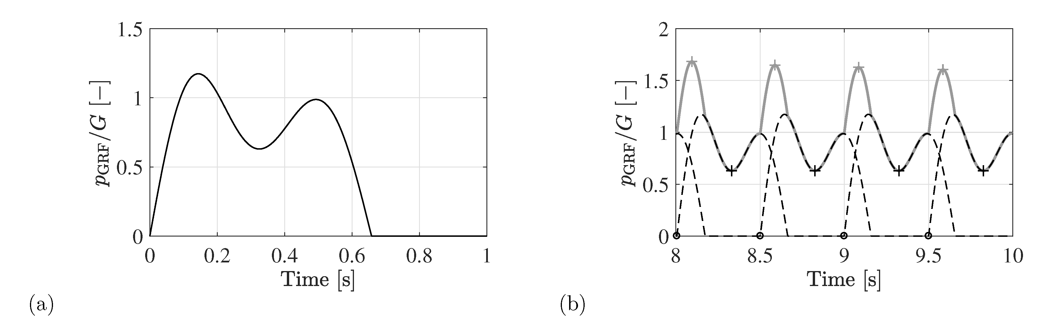
4.1.3. Influence of the Single-Step Load Model

This section investigates the impact of the applied generalised single-step load model in Equations (4) and (5). To this end, the comparison is made between the original GRFs, simulated using the single-step load model introduced by Li et al. [23], and the GRFs reconstructed the single-step load model introduced by Butz [24].
The single-step load models are compared in Figure 8 for a step frequency of 2 Hz. This figure illustrates that the load models display small differences in terms of forcing amplitudes and contact time. Figure 9 shows the amplitude spectrum of the original GRFs and the GRFs reconstructed according to the time-variant pacing rate f s , p and Butz’s single step load model [24]. As a result of using Butz’s model for the reconstruction of the GRFs, the following observations are made (Table 3):
  • The R t 2 coefficient on average reduces with 10%,
  • The R f 2 coefficient on average reduces with 5%.
The small differences in forcing amplitude and contact time result into a reduction of the fit between the original and reconstructed GRFs. The quality of the fit, with an error contained within 15% in the time domain, is considered satisfactory. Furthermore, the quality of the fit for the corresponding amplitude spectrum is very high, with a maximum error of 5% when using the double-stance peaks. As the structural response is much more sensitive to small step-by-step variations in pacing rate than to small step-by-step variations in force amplitude [14,25], the accuracy of the reproduction of the amplitude spectrum is more important than the small step-by-step errors in force amplitude introduced by the applied single-step load model.
In addition, it is noted that using the load model of Li et al. [23] results in larger load amplitudes than when using the load model of Butz [24]. This can be explained by the fact that the model of Li et al. [23] is derived from the design load proposed by Willford and Young [41] representing a 25% probability of exceedance, whereas, to the best of the authors’ knowledge, the load model of Butz [24] represents the average single-step load.

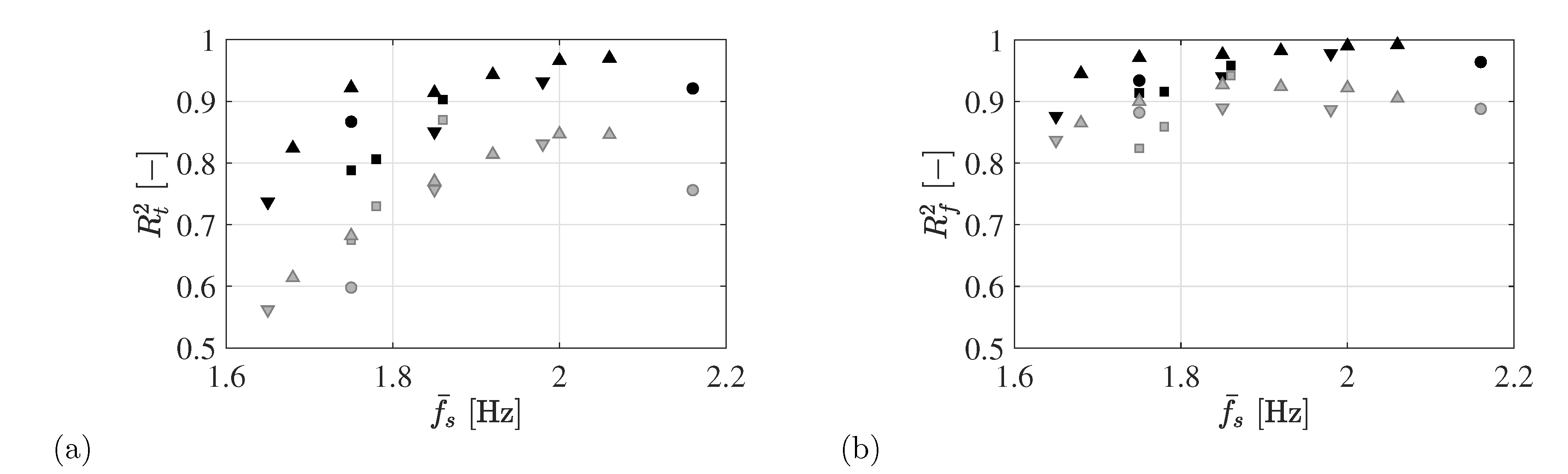
4.2. Application to the Experimentally Registered Body Motion

Finally, the procedure is applied to the dataset described in Section 2. Figure 1b shows a detail of the time history of the registered GRFs and the acceleration levels of the lower back (multiplied by the nominal body mass). From this figure, it is clear that small oscillations at the double-stance peak and single-step dips would prevent to clearly identify the timing of these events from the registered body motion. As proposed in Section 4.1.2, this issue is addressed by applying a lowpass filter with a cut-off frequency of 1.5 × f ¯ s . The corresponding filtered signals are presented in Figure 10.
Next, the processed acceleration signal is used to identify the time-variant pacing rate. The results in Figure 11 show that the actual pacing rate is identified with a high level of accuracy, in particular, when based on the double-stance peaks. For the latter case, the difference between the actual and the identified step frequency of each step are characterized by a mean value of 0.02% and a standard deviation of 2.2 %, respectively.
Then, the GRFs are reconstructed using the procedure detailed in Section 4.1.1 and a single-step load model. At this point, the single-step load model is determined as the average single-step load trace of the participant for the involved treadmill trial, as shown for participant 1 in Figure 12. Figure 13 shows the amplitude spectrum of the true GRFs and the GRFs reconstructed according to the time-variant pacing rate f s , p . This figure shows that a very good fit is obtained between the true and reconstructed GRFs when the reconstruction is based on the double-stance peaks. Table 4 shows that, for the entire range of the walking speeds considered for participant 1, a comparable fit is obtained when the reconstruction is based on the double-stance peaks and the single-stance dips. An average R 2 coefficient of 0.923 and 0.973 is obtained for the fit in time domain and amplitude spectrum, respectively.
When instead, the single-step load model introduced by Butz [24] is applied, the small differences in forcing amplitude and contact ratio causes the R 2 coefficient for the fit in time domain to reduce to an average value of 0.77. However, the fit in the amplitude spectrum is still very good with an average R 2 coefficient of 0.90.
Figure 14 presents the overview of the results obtained for the entire dataset. These results confirm that the use of a generalized single-step load model reduces the accuracy of the reconstructed GRFs. An average fit in the time domain of 0.74 is obtained. More importantly, an average fit of 0.89 is obtained in the amplitude spectrum.
It is concluded that the time-variant pacing rate can be accurately identified from the registered acceleration levels close to the BCoM of the pedestrian. In addition, the GRFs can be estimated with a high level of accuracy when the GRFs are reconstructed based on the identified time-variant pacing rate and a generalised single-step load model: the estimation error on the amplitude spectrum is approximately 10%. Furthermore, it is expected that the error resulting from the use of a generalised single-step load model available in the literature will average out when applied to large groups and crowds with a representative level of intra- and inter-person variability. In terms of the amplitude spectrum, the estimate obtained with the proposed methodology is comparable to the corresponding estimate calculated using the method based on Newton’s second law of motion (Figure 3b and Figure 14b). However, in contrast to applying Newton’s second law, the proposed methodology does not allow for accounting for step-by-step variations in the single-foot forces. This is reflected in the lower values of R t 2 (Figure 3a and Figure 14a).
The results in Figure 11 and Figure 14 also show that the accuracy of the identified pacing rate and reconstructed GRFs decreases for decreasing f ¯ s , and thus decreasing walking speeds. A possible explanation for this observation is the fact that these lower walking speeds were less comfortable for the participants, that is, further away from their self-selected walking speed. Hence, it is expected that, in those cases, the walking behavior and GRFs display more step-by-step irregularities that are less well captured by the proposed methodology.

4.3. Summary

Figure 15 schematically presents the proposed methodology to reconstruct the GRFs from the registered body motion:
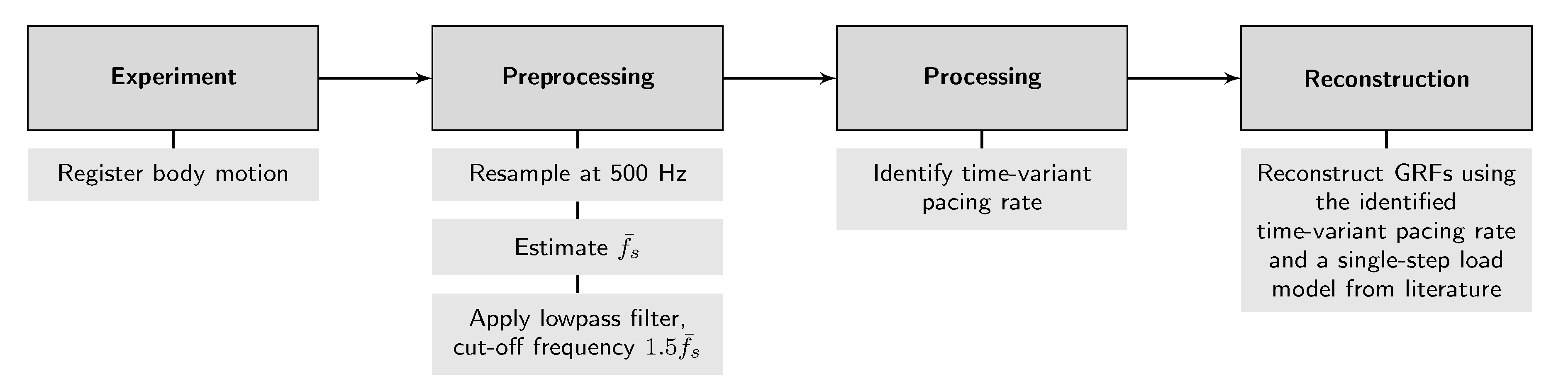
  • An experiment is performed where the body motion of the pedestrian is registered, e.g., the acceleration levels close to the BCoM.
  • The registered body motion data is preprocessed:
    • the data is resampled at at least 500 Hz: Given the accuracy that has to be attained when identifying the time-variant pacing rate ( 1 % ), a resolution in time domain of 0.002 s is recommend. This resolution corresponds to 0.5% of the smallest period of the walking cycle that reasonably can be expected, i.e., corresponding to a step frequency of 2.5 Hz;
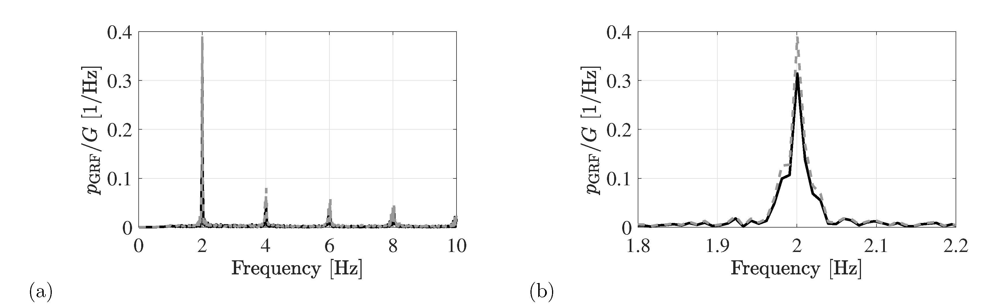
    • the mean step frequency f ¯ s is estimated as the dominant contribution in the PSD of the registered body motion in the relevant frequency range [1.0–2.5] Hz. A frequency resolution of at least 0.05 Hz is recommended;
    • the data is lowpass filtered with a cut-off frequency at 1.5 f ¯ s .
  • The preprocessed data is used to identify the time-variant pacing rate using the method detailed in Section 4.1.1, preferably based on the double-stance peaks. If necessary, apply the appropriate time shift to arrive at an estimate of the actual onset of each step.
  • The GRFs are reconstructed according to Equations (4) and (5).
The benefits of the proposed methodology are the following. The GRFs are reconstructed with a high level of accuracy. The proposed methodology can also be successfully applied when low-cost sensors are used. This results from the fact that the minimum sampling rate of the sensors used to register the body motion is approximately 25 Hz, allowing for accurately capturing the relevant frequency content (0–10 Hz). The registered body motion is then resampled at 500 Hz to obtain a sufficient high resolution in time domain for the subsequent time-domain analysis. A lowpass filter with a cut-off frequency at 1.5 f ¯ s is applied to the registered (resampled) body motion, making the methodology robust against measurement noise. The methodology furthermore allows for accurately identifying the time-variant pacing rate from the registered body motion through the identification of the time between the nominally identical events of successive walking cycles. This means that the proposed procedure can be applied to the registered body motion, regardless of the position of the sensor on the human body. The only requirement is that the events identified from the registered body motion can be uniquely matched to the corresponding nominally identical event in the walking cycle. Finally, it is observed that the estimation errors mainly result from (small) differences in the step-by-step load amplitude and contact time and not from estimation errors on the time-variant pacing rate. This is an important observation as the structural response is predominantly sensitive to variations of the pacing rate for successive footfalls.

5. Conclusions

This paper introduces a methodology to reconstruct the vertical GRFs from the registered body motion, which is reasonably robust against measurement noise arising from soft-tissue artefacts and the application of low-cost sensor technologies. The vertical GRFs are reconstructed from the experimentally identified time-variant pacing rate and a generalised single-step load model available in the literature. It is shown that the time-variant pacing rate can be identified with a high level of accuracy from the registered body motion. As the proposed methodology applies a lowpass filter with a cut-off frequency at 1.5 times, the average pacing rate of the person to minimise the influence of measurement noise on the registered body motion, it can also be successfully applied when low-cost sensors are used. Furthermore, the proposed procedure can be applied to the registered body motion, regardless of the position of the sensor on the human body. The only requirement is that the events identified from the registered body motion can be uniquely matched to the corresponding nominally identical event in the walking cycle.
It is shown that, when using the experimentally identified pacing rate and an individually identified single-step load model, the GRFs can be reconstructed with a very high level of accuracy: the estimation error on the amplitude spectrum is close to 5%. Due to the use of a generalised single-step load model available in the literature, the estimation error increases to approximately 10%. These estimation errors mainly result from small differences in the step-by-step load amplitude and contact time and not from estimation errors in the time-variant pacing rate. It can be expected that the error resulting from the use of a generalised single-step load model available in the literature will average out when applied to large groups and crowds with a representative level of intra- and inter-person variability. When the impact of soft-tissue artefacts is low, a comparable estimate can be obtained using Newton’s second law of motion. The proposed methodology furthermore has the benefit that only the time between successive cycles, and not the exact magnitude of the registered body motion, is of interest. This advantage is interesting for the application of low-cost sensors that are characterised by a relatively low sensitivity, and, therefore, for application in situ when a large number of persons is involved.
The present study uses generalised single-step load models available in the literature. These load models are determined for the walking load induced on a rigid floor. This implies that the reconstructed GRFs represent the pedestrian load induced without any impact of HSI. When the proposed methodology would be applied to replicate in situ experiments, the impact of HSI can be determined by investigating the difference between the observed structural response (with HSI) and the one predicted using the reconstructed GRFs (without HSI).

Author Contributions

Conceptualization, Methodology, Investigation, Visualization, Writing—Original Draft Preparation, K.V.N.; Experimental Work, Biomechanics, G.Z. and A.S.; Supervision, P.V.d.B.

Funding

The first author is a postdoctoral fellow of the Research Foundation Flanders (FWO, 12E0816N). The financial support is gratefully acknowledged.

Conflicts of Interest

The authors declare no conflict of interest.

Abbreviations

The following abbreviations are used in this manuscript:
BCoMBody Centre of Mass
CoMCentre of Mass
GRFsGround Reaction Forces
HSIHuman–Structure Interaction
PSDPower Spectral Density

References

  1. Živanović, S.; Pavić, A.; Reynolds, P. Vibration serviceability of footbridges under human-induced excitation: A literature review. J. Sound Vib. 2005, 279, 1–74. [Google Scholar] [CrossRef] [Green Version]
  2. Association Française de Génie Civil, Sétra/AFGC. Sétra: Evaluation du Comportement Vibratoire des Passerelles Piétonnes Sous L’action des Piétons (Assessment of Vibrational Behaviour of Footbridges Under Pedestrian Loading); AFGC: Paris, France, 2006. [Google Scholar]
  3. Heinemeyer, C.; Butz, C.; Keil, A.; Schlaich, M.; Goldack, A.; Lukić, M.; Chabrolin, B.; Lemaire, A.; Martin, P.; Cunha, A.; Caetano, E. Design of Lightweight Footbridges for Human Induced Vibrations—Background Document in Support to the Implementation, Harmonization and Further Development of the Eurocodes; JRC-ECCS 2009; EU Publications: Luxembourg, 2009. [Google Scholar]
  4. Georgakis, C.T.; Ingólfsson, E. Recent advances in our understanding of vertical and lateral footbridge vibrations. In Proceedings of the 5th International Footbridge Conference, London, UK, 6–18 July 2014. [Google Scholar]
  5. Venuti, F.; Racic, V.; Corbetta, A. Modelling framework for dynamic interaction between multiple pedestrians and vertical vibrations of footbridges. J. Sound Vib. 2016, 379, 245–263. [Google Scholar] [CrossRef]
  6. Zang, M.; Georgakis, C.; Chen, J. Biomechanically Excited SMD Model of a Walking Pedestrian. J. Bridge Eng. 2016, 21. [Google Scholar] [CrossRef]
  7. Shahabpoor, E.; Pavić, A.; Racić, V. Interaction between Walking Humans and Structures in Vertical Direction: A Literature Review. Shock Vib. 2016, 12–17. [Google Scholar] [CrossRef]
  8. Dang, H.; Živanović, S. Influence of Low-Frequency Vertical Vibration on Walking Locomotion. J. Struct. Eng. 2016. [Google Scholar] [CrossRef]
  9. Van Nimmen, K.; Lombaert, G.; De Roeck, G.; Van den Broeck, P. The impact of vertical human–structure interaction on the response of footbridges to pedestrian excitation. J. Sound Vib. 2017, 402, 104–121. [Google Scholar] [CrossRef]
  10. Živanović, S. Benchmark footbridge for vibration serviceability assessment under vertical component of pedestrian load. J. Struct. Eng. 2012, 138, 1193–1202. [Google Scholar] [CrossRef]
  11. McDonald, M.; Živanović, S. Measuring ground reaction force and quantifying variability in jumping and bobbing actions. J. Struct. Eng. 2017, 143. [Google Scholar] [CrossRef]
  12. Racić, V.; Brownjohn, J.M.W.; Pavić, A. Reproduction and application of human bouncing and jumping forces from visual marker data. J. Sound Vib. 2010, 329, 3397–3416. [Google Scholar] [CrossRef]
  13. Carroll, S.P.; Owen, J.S.; Hussein, M.F.M. Reproduction of lateral ground reaction forces from visual marker data and analysis of balance response while walking on a laterally oscillating deck. Eng. Struct. 2013, 49, 1034–1047. [Google Scholar] [CrossRef]
  14. Van Nimmen, K.; Lombaert, G.; Jonkers, I.; De Roeck, G.; Van den Broeck, P. Characterisation of walking loads by 3D inertial motion tracking. J. Sound Vib. 2014, 333, 5212–5226. [Google Scholar] [CrossRef]
  15. Toso, M.; Gomes, H.; da Silva, F.; Pimentel, R. Experimentally fitted biodynamic models for pedestrian-structure interaction in walking situations. Mech. Syst. Signal Process. 2015, 72–73, 590–606. [Google Scholar] [CrossRef]
  16. Bocian, M.; Brownjohn, J.; Racic, V.; Hester, D.; Quattrone, A.; Monnickendam, R. A framework for experimental determination of localised vertical pedestrian forces on full-scale sturctures using wireless attitude and heading reference systems. J. Sound Vib. 2016, 376, 217–243. [Google Scholar] [CrossRef] [Green Version]
  17. Brownjohn, J.; Bocian, M.; Hester, D.; Quattrone, A.; Hudson, W.; Moore, D.; Goh, S.; Lim, M. Footbridge system identification using wireless inertial measurement units for force and response measurements. J. Sound Vib. 2016, 384, 339–355. [Google Scholar] [CrossRef]
  18. Bocian, M.; Brownjoh, J.; Racić, V.; Hester, D.; Quattrone, A.; Gilbert, L.; Beasley, R. Time-dependent spectral analysis of interactions within groups of walking pedestrians and vertical structural motion using wavelets. Mech. Syst. Signal Process. 2018, 105, 502–523. [Google Scholar] [CrossRef]
  19. Brownjoh, J.; Chen, J.; Bocian, M.; Racić, V.; Shahabpoor, E. Using inertial measurement units to identify medio-lateral ground reaction forces due to walking and swaying. J. Sound Vib. 2018, 426, 90–110. [Google Scholar] [CrossRef]
  20. Dang, H.; Živanović, S. Experimental characterisation of walking locomotion on rigid level surfaces using motion capture system. Eng. Struct. 2015, 91, 141–154. [Google Scholar] [CrossRef]
  21. Nigg, B.M.; Herzog, W. Biomechanics of the Musculo-Skeletal System, 3rd ed.; Wiley: New York, NY, USA, 2007. [Google Scholar]
  22. Shahabpoor, E.; Pavic, A.; Brownjohn, J.; Billings, S.; Guo, L.; Bocian, M. Real-life measurement of tri-axial walking ground reaction forces using optimal network of wearable inertial measurement units. IEEE Trans. Neural Syst. Rehabil. Eng. 2018, 26, 1243–1253. [Google Scholar] [CrossRef] [PubMed]
  23. Li, Q.; Fan, J.; Nie, J.; Li, Q.; Chen, Y. Crowd-induced random vibration of footbridge and vibration control using multiple tuned mass dampers. J. Sound Vib. 2010, 329, 4068–4092. [Google Scholar] [CrossRef]
  24. Butz, C. Beutrag zur Berechnung Fussgängerinduzierter Brückenschwingungen—Shaker Verlag (Contribution to the Determination of Pedestrian Induced Bridge Vibrations). Ph.D. Thesis, RWTH Aachen, Aachen, Germany, 2006. [Google Scholar]
  25. Middleton, C. Dynamic Performance of High Frequency Floors. Ph.D. Thesis, University of Sheffield, Sheffield, UK, 2009. [Google Scholar]
  26. Duysens, J.; Jonkers, I.; Verschueren, S. MALL: Movement & Posture Analysis Laboratory Leuven; Interdepartmental Research Laboratory at the Faculty of Kinisiology and Rehabilitation Sciences: Leuven, Belgium.
  27. Racić, V.; Pavić, A.; Reynolds, P. Experimental identification and analytical modelling of walking forces: A literature review. J. Sound Vib. 2009, 326, 1–49. [Google Scholar] [CrossRef]
  28. Paolini, G.; Croce, U.; Riley, P.; Neuwton, F.; Kerrigan, D. Testing of a tri-instrumented-treadmill unit for kinetic analysis of locomotion tasks in static and dynamic loading conditions. Med. Eng. Phys. 2007, 29, 404–411. [Google Scholar] [CrossRef]
  29. MATLAB. R2015b, The MathWorks Inc.: Natick, MA, USA, 2015.
  30. Van den Bogert, A.; Read, L.; Nogg, B. A method for inverse dynamic analysis using accelerometry. J. Biomech. 1996, 29, 949–954. [Google Scholar] [CrossRef]
  31. Liikavainio, T.; Bragge, T.; Hakkarainen, M.; Jurvelin, J.; Karjalainen, P.; Arokoski, J. Reproducibility of loading measurements with skin-mounted accelerometers during walking. Arch. Phys. Med. Rehabil. 2007, 88, 907–915. [Google Scholar] [CrossRef]
  32. Vicon Motion Systems. Vicon Motion Systems Product Manuals; Vicon Motion Systems: Oxford, UK.
  33. CODAmotion. Technical Data Sheet; Charnwood Dynamics: Rothley, UK, 2012. [Google Scholar]
  34. Xsens Technologies B.V. MTw User Manual; Xsens: Enschede, The Netherlands, 2010. [Google Scholar]
  35. Draper, N.; Smith, H. Applied Regression Analysis; Wiley: New York, NY, USA, 1998. [Google Scholar]
  36. Denoth, J. Chapter: Load on the locomotor system and modelling. In Biomechanics of Running Shoes; Nigg, B., Ed.; Human Kinetics Publishers: Champaign, IL, USA, 1986; pp. 63–116. [Google Scholar]
  37. Silva, F.; Pimentel, R. Biodynamic walking model for vibration serviceability of footbridges in vertical direction. In Proceedings of the 8th International Conference on Structural Dynamics of EURODYN, Leuven, Belgium, 4–6 July 2011. [Google Scholar]
  38. Silva, F.; Brito, H.; Pimentel, R. Modeling of crowd load in vertical direction using biodynamic model of pedestrians crossing footbridges. Can. J. Civ. Eng. 2014, 41, 1196–1204. [Google Scholar] [CrossRef]
  39. Racić, V.; Pavić, A. Mathematical model to generate near-periodic human jumping force signals. Mech. Syst. Signal Process. 2010, 24, 138–152. [Google Scholar] [CrossRef]
  40. Young, P. Improved floor vibration prediction methodologies. ARUP Vibration Seminar, 2001. [Google Scholar]
  41. Willford, M.R.; Field, C.; Young, P. Improved methodologies for the prediction of footfall-induced vibration. In Proceedings of the SPIE 2005, San Diego, CA, USA; pp. 1–15.
  42. Butz, C.; Feldmann, M.; Heinemeyer, C.; Sedlacek, G. SYNPEX: Advanced Load Models for Synchronous Pedestrian Excitation and Optimised Design Guidelines for Steel Footbridges; Technical Report, Research Fund for Coal and Steel; EU Publications: Luxembourg, 2008. [Google Scholar]
Figure 1. Time series of the GRFs normalised to G for a walking speed of 5.5 km/h: (a) relevant time window; (b) detail of the time history; measurements (black, solid) and reconstructed using Newton’s second law (grey, dashed).
Vibration 01 00018 g001
Figure 2. Amplitude spectrum of the GRFs: (a) frequency range of interest; (b) zoom around f ¯ s ; measurements (black, solid) and reconstructed using Newton’s second law (grey, dashed).
Vibration 01 00018 g002
Figure 3. R t 2 and R f 2 for the GRFs reconstructed using Newton’s second law for participant 1 (∆); participant 2 (□); participant 3 (∘) and participant 4 (▽), in terms of f ¯ s .
Vibration 01 00018 g003
Figure 4. (a) the single-step load model defined by Li et al. [23] for a step frequency of 2 Hz and (b) the vertical single-step foot traces (dashed) and the corresponding sum (solid): actual onset of each step (∘), double-stance peaks (+, grey), single-step dips (+, black).
Vibration 01 00018 g004
Figure 5. The original GRFs (black, solid) and the reconstructed GRFs based on the single-step load model and the time-variant pacing rate identified from the double-stance peaks (grey, dashed).
Vibration 01 00018 g005
Figure 6. Amplitude spectrum of the GRFs: (a) frequency range of interest; (b) zoom around f ¯ s ; original GRFs (black, solid) and reconstructed GRFs based on the single-step load model derived for the participant and the time-variant pacing rate identified from the double-stance peaks (grey, dashed).
Vibration 01 00018 g006
Figure 7. Amplitude spectrum of the GRFs: (a) frequency range of interest; (b) zoom around f ¯ s ; original GRFs (black, solid) and reconstructed GRFs based on the single-step load model derived for the participant and the time-variant pacing rate identified from the lowpass filtered input signal according to the double-stance peaks (grey, dashed).
Vibration 01 00018 g007
Figure 8. For a step frequency of 2 Hz: the single-step load model defined by Li et al. [23] (black, solid) and Butz [24] (grey, dashed).
Vibration 01 00018 g008
Figure 9. Amplitude spectrum of the GRFs: (a) frequency range of interest; (b) zoom around f ¯ s ; original GRFs (black, solid) and reconstructed GRFs using the generalised single-step load model of Butz [24] and the double-stance peaks (grey, dashed).
Vibration 01 00018 g009
Figure 10. Detail of the time history of (a) the measured GRFs and (b) the measured acceleration levels on the lower back normalised to g, after applying a lowpass filter with a cut-off frequency at 12 Hz (grey, dashed) and 1.5 × f ¯ s (black, solid) and the corresponding double-stance peaks (∘) and single-step dips (+).
Vibration 01 00018 g010
Figure 11. The mean value μ and standard deviation σ of the difference between the actual and the identified step frequency of each step Δ f s based on the double-stance peaks (black) and the single-step dips (gray), for participant 1 (∆), participant 2 (□), participant 3 (∘) and participant 4 (▽), in terms of f ¯ s .
Vibration 01 00018 g011
Figure 12. For a step frequency of 2 Hz: the single-step load model derived for participant 1 (black, solid) and defined by Butz [24] (grey, dashed).
Vibration 01 00018 g012
Figure 13. PSD of the GRFs: (a) frequency range of interest, (b) zoom around f ¯ s ; measured GRFs (black, solid) and GRFs reconstructed using the time-variant pacing rate identified from the double-stance peaks and the single-step load model derived for the participant (dash-dot) and defined by by Butz [24] (dashed).
Vibration 01 00018 g013
Figure 14. R t 2 and R f 2 for the GRFs reconstructed using the identified time-variant pacing rate, and the single-step load model derived for the participant (black, solid) and defined by Butz [24] (grey, dashed), for participant 1 (∆), participant 2 (□), participant 3 (∘) and participant 4 (▽), in terms of f ¯ s .
Vibration 01 00018 g014
Figure 15. Schematic representation of the proposed methodology to reconstruct the GRFs from the registered body motion.
Vibration 01 00018 g015
Table 1. Information on the persons involved in the treadmill trials.
ParticipantSexAgeHeight [m]Mass [kg]Considered Treadmill Speeds [m/s]
1female261.6552[0.97, 1.11, 1.25, 1.39, 1.53, 1.67]
2male231.8172[1.11, 1.25, 1.39]
3male271.7566[1.1, 1.7]
4male241.8072[1.0, 1.3, 1.6]
Table 2. For each of the treadmill trials of participant 1: the walking speed v s , the identified average step frequency f ¯ s and effective mass fraction α ¯ eff , the corresponding coefficients of determination R t 2 and R f 2 for the GRFs reconstructed using Newton’s second law.
v s f ¯ s α ¯ eff R t 2 [-] R f 2 [-]
[ km / h ] [Hz][-]m α ¯ eff m m α ¯ eff m
3.51.680.780.8610.9420.9030.973
4.01.750.760.8570.9550.8930.981
4.51.850.760.8640.9620.8960.986
5.01.920.760.8690.9590.9000.982
5.52.000.740.8630.9620.8900.982
6.02.060.740.8720.9630.8960.981
Average0.8600.9510.8950.976
Table 3. For each of the numerically simulated cases: the average step frequency f ¯ s , the difference between the actual and the identified step frequency Δ f s , p = ( f s f s , p ) / f ¯ s and Δ f s , d = ( f s f s , d ) / f ¯ s with mean μ and standard deviation σ , and the corresponding coefficients of determination R t 2 and R f 2 .
f ¯ s [ Hz ] Δ f s , p [%] Δ f s , d [%] R t 2 [-] R f 2 [-]
μ σ μ σ f s , p f s , d f s , p f s , d
1.50.021.05000.98810.9971
1.60.011.09000.98910.9971
1.70.021.02000.99210.9981
1.80.010.97000.99410.9981
1.90.021.00000.99410.9981
20.020.87000.99510.9981
2.10.011.01000.99410.9981
Average0.0161.001000.99210.9981
Influence of a cut-off frequency at 2.5 × f ¯ s
1.50.020.740.112.350.9940.9490.9980.974
1.60.010.680.132.470.9960.9580.9990.975
1.70.010.660.091.930.9970.9780.9990.986
1.80.010.610.091.780.9980.9840.9990.989
1.90.010.620.071.540.9980.9890.9990.993
20.010.570.051.230.9980.9930.9990.996
2.10.020.740.051.200.9970.9940.9990.996
Average0.010.660.081.790.9990.980.9990.990
Influence of a cut-off frequency at 1.5 × f ¯ s
1.50.010.840.010.710.9930.9950.9990.998
1.60.010.810.010.640.9940.9960.9990.999
1.70.010.830.010.610.9950.9970.9990.999
1.80.010.730.010.610.9960.9970.9990.999
1.90.010.750.010.570.9970.9980.9990.999
20.021.100.010.550.9930.9980.9980.999
2.10.021.030.010.510.9940.9980.9990.999
Average0.010.870.010.600.9950.9970.9990.999
Influence of the single-step load model
1.5====0.9030.9050.9490.951
1.6====0.90.9030.9510.952
1.7====0.9190.920.9540.955
1.8====0.9150.9150.9510.951
1.9====0.8910.8890.9510.952
2====0.8530.8580.9480.95
2.1====0.8590.8570.9550.956
Average 0.8910.8920.9510.952
Table 4. For each of the treadmill trials of participant 1: the walking speed v s , the identified average step frequency f ¯ s , the difference between the actual and the identified step frequency Δ f s , p = ( f s f s , p ) / f ¯ s and Δ f s , d = ( f s f s , d ) / f ¯ s with mean μ and standard deviation σ , and the corresponding coefficients of determination R t 2 and R f 2 .
v s f ¯ s Δ f s , p [%] Δ f s , d [%] R t 2 [-] R f 2 [-]
[ km / h ] [Hz] μ σ μ σ f s , p f s , d f s , p f s , d
3.51.680.011.550.507.800.8240.8550.9450.930
41.750.031.540.397.630.9220.8940.9710.958
4.51.850.011.380.305.960.9140.9230.9760.970
51.920.001.200.184.150.9430.9540.9820.980
5.52.000.011.440.133.410.9660.9630.9900.988
62.060.001.510.082.510.9700.9530.9920.980
Average0.011.440.265.240.9230.9240.9760.968
3.51.68====0.6140.6450.8650.837
41.75====0.6820.7130.9000.887
4.51.85====0.7700.7800.9270.917
51.92====0.8140.8270.9240.921
5.52.00====0.8470.8430.9220.919
62.06====0.8460.8280.9050.912
Average====0.7620.7730.9070.899

