Evaluation of Shock Detection Algorithm for Road Vehicle Vibration Analysis

Abstract

The ability to characterize shocks which occur during road transport is a vital prerequisite for the design of optimized protective packaging, which can assist in reducing cost and waste related to products and good transport. Many methods have been developed to detect shocks buried in road vehicle vibration signals, but none has yet considered the nonstationary nature of vehicle vibration and how, individually, they fail to accurately detect shocks. Using machine learning, several shock detection methods can be combined, and the reliability and accuracy of shock detection can also be improved. This paper presents how these methods can be integrated into four different machine learning algorithms (Decision Tree, k-Nearest Neighbors, Bagged Ensemble, and Support Vector Machine). The Pseudo-Energy Ratio/Fall-Out (PERFO) curve, a novel classification assessment tool, is also introduced to calibrate the algorithms and compare their detection performance. In the context of shock detection, the PERFO curve has an advantage over classical assessment tools, such as the Receiver Operating Characteristic (ROC) curve, as it gives more importance to high-amplitude shocks.

1. Introduction

In most countries, product distribution predominantly relies on road transportation. This type of transportation can be harmful to freight as the interaction between the road vehicle and pavements creates shocks and vibration. To mitigate this problem, a common practice is to use protective packaging, which significantly increases shipping costs. Inefficient packaging constitutes a pressing global problem that costs hundreds of billions of dollars, and also impacts negatively upon the environment. An insufficient level of packaging increases the occurrence of product damage during transport, whereas excessive packaging increases the packages’ weight and volume, which creates more costs throughout the supply chain. In order to reduce these costs, packaging protection is currently being optimized by simulating the vibration produced by road vehicles. Different physical simulation methods are prescribed by international and national standards [1,2,3,4]. The model used by the standards assumes that Road Vehicle Vibration (RVV) is a Gaussian and stationary random signal. It is broadly acknowledged that this assumption oversimplifies the RVV, which imposes a significant limit onto packaging optimization [5,6,7,8,9]. Realistic and accurate RVV simulations must consider the different excitation modes contained in RVV—that is, the nonstationary random vibration induced by the pavement’s profile and variations in vehicle speed, as well as the shocks caused by the pavement’s aberrations. More complex RVV models have been recently developed to enhance RVV simulations by essentially using two different approaches—analyzing RVV in the time domain [6,8,10,11,12,13,14,15,16,17,18,19], and in the time-frequency domain [20,21,22,23,24,25,26,27]. However, a fundamental problem still remains; these alternatives are effective only in specific scenarios, such as: (1) when the underlying random vibrations are stationary (which is rarely the case for RVVs), or; (2) when the random vibrations are non-stationary and no shocks are present. No single approach available today can accurately detect shocks that are superimposed on non-stationary, random background vibrations. Both excitation modes should be included in the RVV simulation to ensure that simulations are realistic and accurate and that the packaging will protect against vibrations during transport without being too excessive. Each mode is represented by a different mathematical model and cannot be analyzed with the same statistical tools. For instance, the nonstationary mode can be modelled as a series of stationary Gaussian random segments of different RMS (root mean square) values [6], and the shocks as a distribution of impulses of different amplitudes. To create these models, the nonstationary random vibration and the shocks have to be characterized separately. This task is challenging because all the excitation modes co-exist in the vibration acceleration signal recorded on a vehicle.

This paper assesses different machine learning classifiers to index the shocks buried in synthetic, nonstationary, random vibration signals representing real RVV. With machine learning, it is possible to integrate many RVV analysis methods, such as moving statistics, the Discrete Wavelet Transform, and the Hilbert-Huang Transform, which greatly enhance shock detection. The processing required to integrate these methods of analysis is presented in the first part of this paper. The second part deals with an evaluation of four classification algorithms (Decision Tree, k-Nearest Neighbors, Bagged Ensemble, and Support Vector Machine) which was performed using synthetically generated RVV signals. The evaluation used a novel detection assessment tool, namely the PERFO (Pseudo Energy Ration/Fall-Out) curve, which was specifically developed for shock detection purposes. The application of this machine learning algorithm on real-life vehicle measurements was described in detail in a previous publication by the authors [28].

2. RVV Analysis Methods

RVV signals can be studied by using time and time-frequency analysis tools. Attempts at detecting shocks have been made using moving statistics, such as moving RMS [11,12], moving kurtosis [12], and the moving crest factor [8,10,11,12,13,14,15], calculated on RVV acceleration signals in the time domain. Using different moving window length, the moving RMS has also been used to describe the RVV nonstationarities as a series of stationary Gaussian random segments [6,8,15,16,17,18]. The sensitivity of these moving statistics to shocks and nonstationarities highly depends of the window length used in the calculation [29,30]. For instance, short windows have good sensitivity to shocks, but cannot distinguish shocks for a short, stationary Gaussian random segment. As the nonstationarities and shocks may cause variations in the RVV spectrum [7,31,32,33], different time-frequency analysis methods have been used to make this distinction. One of these methods is the Discrete Wavelet Transform (DWT), which is often used to identify shocks [20,21,22,23] and RVV nonstationary components [22,23,24]. The DWT has good sensitivity to signal state changes and shocks but also to nonstationary segment changes, which may create similar output in a DWT scalogram [22]. The Hilbert-Huang transform, which is an adaptive time-frequency analysis method [34], has also been used to analyze both modes of RVV signals [23,25,26,27]. This method has better sensitivity to nonstationary segments than the DWT [23,25], but cannot be effectively used to detect shocks [25,27].

All these methods have their own benefits and limitations when applied to RVV signals, but none can effectively detect shocks buried in nonstationary, random vibration signals. A useful approach which can get the most out of the time and time-frequency tools is to integrate them with machine learning by using a classification algorithm [30]. As shown in Figure 1, the process starts with a learning dataset, which is a set of data where the classes are known. For RVV, this is a vertical acceleration signal where the locations of the shocks are known. Dataset segments containing shocks are attributed to the class “shocks”, and the remaining to the class “no shock”. The dataset is processed to reveal different data behaviors and characteristics in a format compatible with machine learning algorithms. This is where machine learning is different to other classification approaches, because it can base its prediction on several different signal processing methods. This means it can combine the more effective shocks and nonstationary analysis methods to distinguish the shocks from signal intensity variations (nonstationarity). The outcomes of each method are called predictors. Once the processing is completed, the data is randomly partitioned into two sets: the training dataset, and the validation set, where both sets have the same proportion of classes. The training dataset is used to train the algorithm and develop the classifier, and the trained classifier is then validated using the validation dataset. The outcome of the validation phase is applied to optimize the performance of various algorithms, and the optimized algorithm is then employed to generalize the classification model to a new dataset.

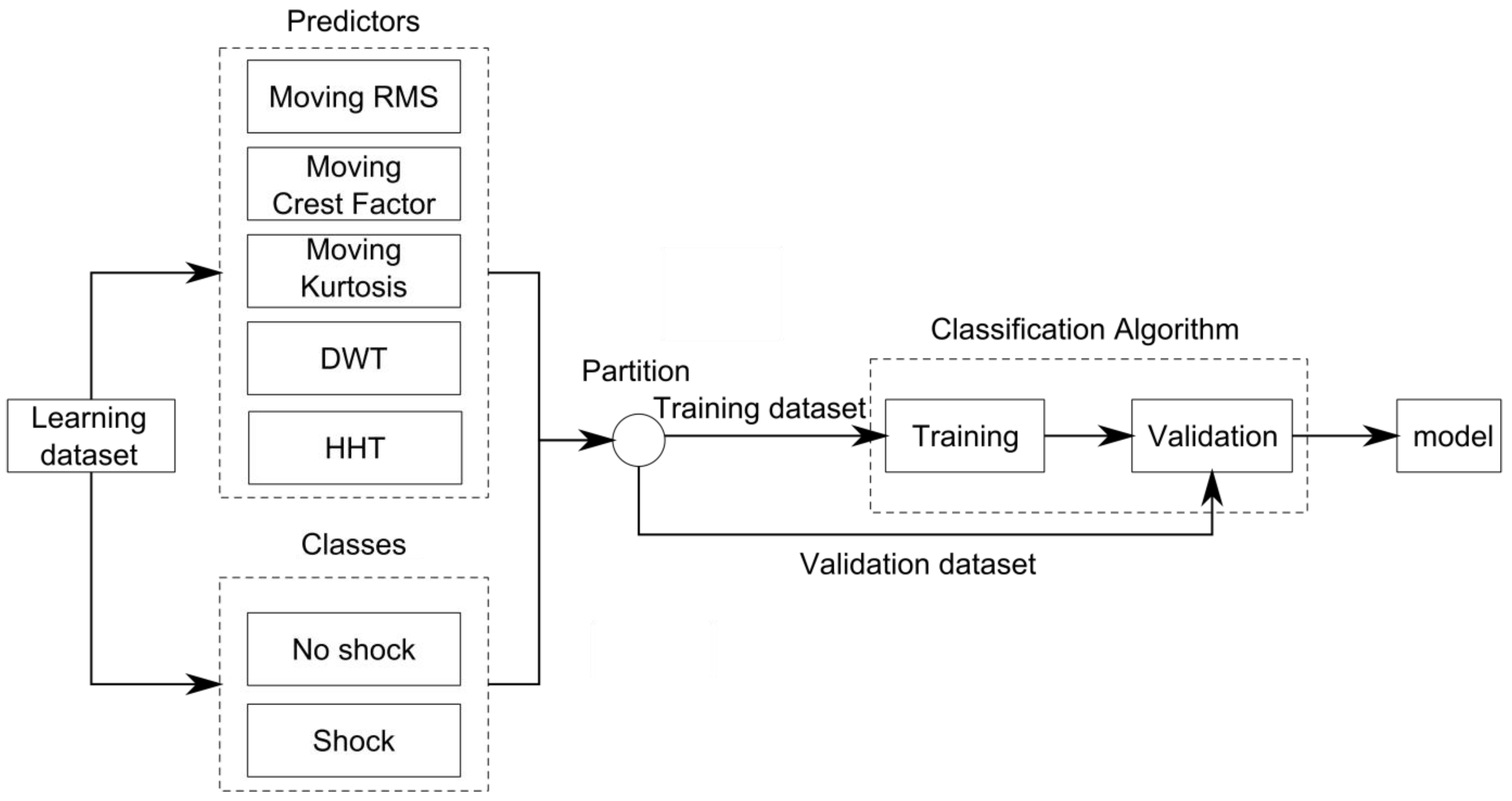
2.1. Machine Learning Algorithms

There exists a large variety of machine learning algorithms, which have a myriad of potential applications. Based on preliminary work undertaken by Lepine [35], four different machine learning classifiers have been selected for RVV shock detection purposes, such as the Decision Tree, k-Nearest Neighbors (kNN), Bagged Ensemble, and Support Vector Machine (SVM). These algorithms were trained using their implementation in Matlab^® (for more information, refer to Hastie et al. [36], Rogers and Girolami [37], Cherkassky and Mulier [38], and Shalev-Shwartz and Ben-David [39]).

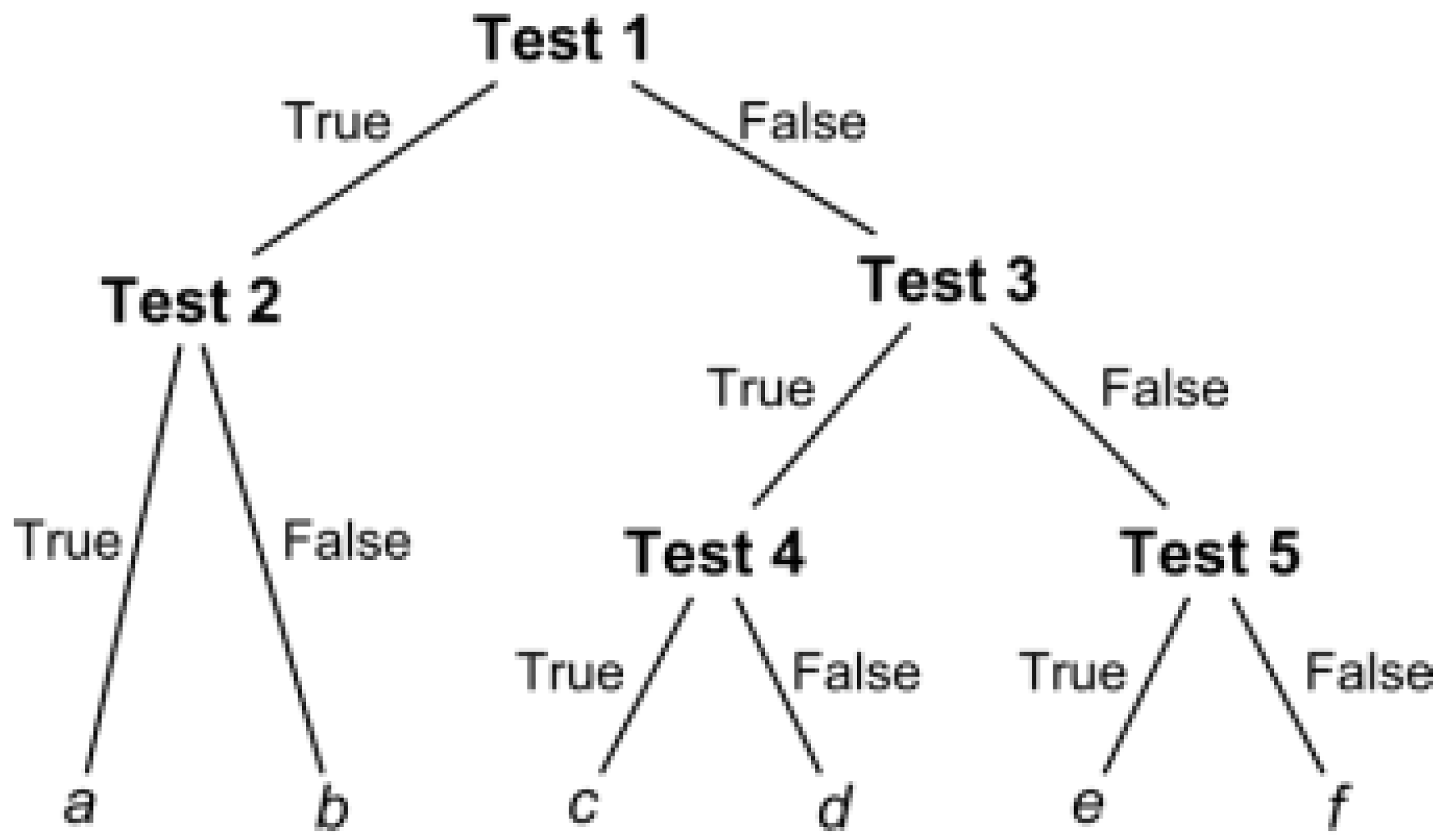
2.1.1. Decision Tree

The Decision Tree algorithms base their prediction on a cascade of statistical tests, where the outcome of the first test leads to another test and so on until the class of the data is predicted (Figure 2). The predictors are the statistics used for the tests. For shock detection application, a Decision Tree comprised of 20 tests was used, as this was found to be optimal by Lepine [35].

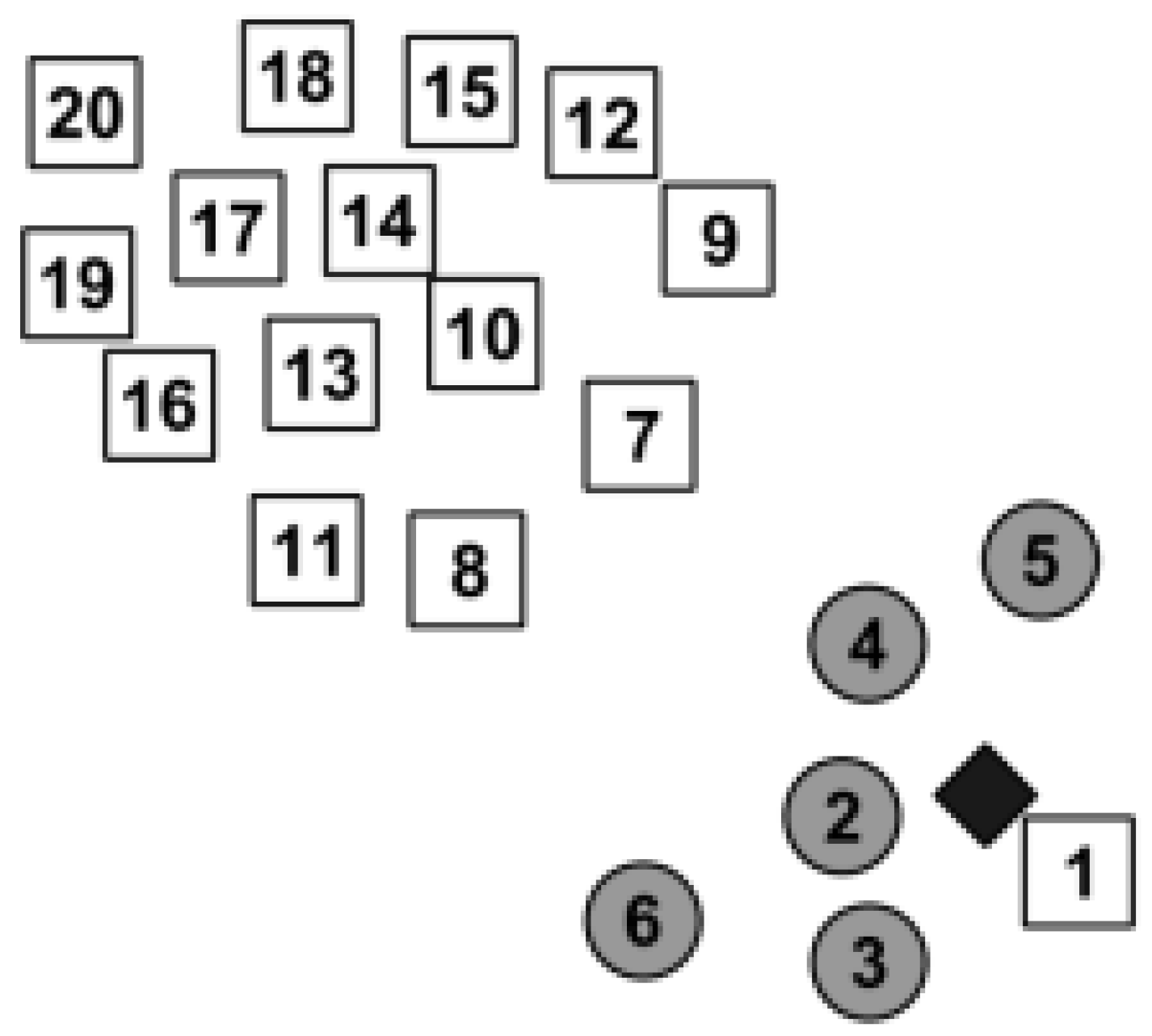
2.1.2. k-Nearest Neighbors

The k-Nearest Neighbors algorithms (kNN) are able to group training datasets by class in as many spaces as there are predictors. A kNN algorithm classifies new data points by grouping them into the most common class of their nearest k neighbors; in other words, the classification is made by association. If the majority of a data point’s nearest neighbors belong to one class, it is more likely that the point belongs to this class too. For instance, in Figure 3, 15 data points are squares, five are circles, and the lozenge class is unknown. As four of the five nearest neighbors of the lozenge are circles, a 5-Nearest Neighbors (5NN) classifier would classify this data point as a circle. For the shock detection application, a 100NN algorithm was used, as recommended by Lepine [35]. The Euclidean distance was used to define the nearest neighbors.

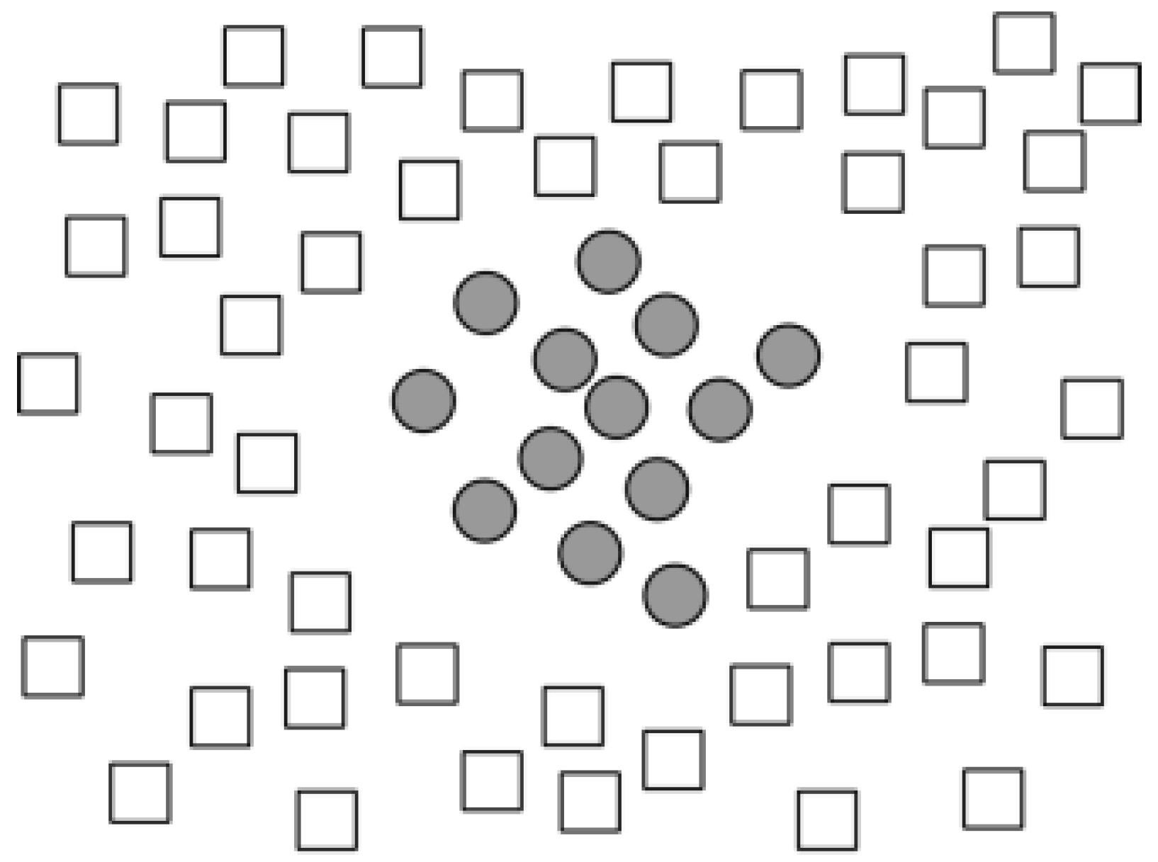
2.1.3. Bagged Ensemble

Bagged ensemble algorithms use a combination of Decision Trees on which they base their prediction. Bagged algorithm stands for “bootstrap aggregation”, and generates Decision Trees on different random data samples. The classification is made by using the average response of each of these Decision Trees, and an ensemble of 150 decision trees was found to be suitable for shock-detection purposes.

2.1.4. Support Vector Machine

$D\left(x\right)={\displaystyle \sum _{i=1}^n{\stackrel{⌢}{\alpha }}_i{y}_i\left(x\cdot x\prime \right)}+\stackrel{⌢}{b}$ Support Vector Machine (SVM) algorithms are powerful classifiers that only work when the data have only two classes. As such, they are well-suited for shock detection. Using a training dataset, the SVM found a hyperplane that maximized the distance between the two classes’ data points represented in all their dimensions (predictors). This hyperplane is defined as:

$$D\left(x\right)={\displaystyle \sum }_{i=1}^n{\stackrel{⌢}{\alpha }}_i{y}_i\left(x\cdot x\prime \right)+\stackrel{⌢}{b}$$

(1)

where $\left(x_i,y_i\right)$, for $i=1,\dots ,n$ are, respectively, the predictor matrix and class vector of the n training data points; $\left(x\cdot x\prime \right)$ is the predictor-matrix inner product; and ${\stackrel{⌢}{\alpha }}_i$ and $\stackrel{⌢}{b}$ are parameters defined during the learning process [36,37,38,39].

There are many cases where it is impossible to solve (1) in its direct form because no single hyperplane can separate the data classes. For example, the dataset shown in Figure 4 cannot be divided by a single hyperplane because the cluster of circles is surrounded by squares.

This type of problem can be solved using nonlinear transformation by means of Kernel functions which transform the data into a space where the classes are more distinct. This process is done by replacing the inner product in the linear hyperplane definition by a nonlinear Kernel function, $G\left(x,x\prime \right)$, such as:

$$D\left(x\right)={\displaystyle \sum }_{i=1}^n{\stackrel{⌢}{\alpha }}_i{y}_{i}G\left(x\cdot x\prime \right)+\stackrel{⌢}{b}$$

(2)

The Kernel function that was found to be well-suited for shock detection purposes is the Gaussian functions (also known as the radial basic functions):

$$G\left(x,x\prime \right)=\exp \left\{-\frac{{\left|x-x\prime \right|}^2}{{\sigma }^2}\right\}$$

(3)

where ${\sigma }^2$ defines the function’s width.

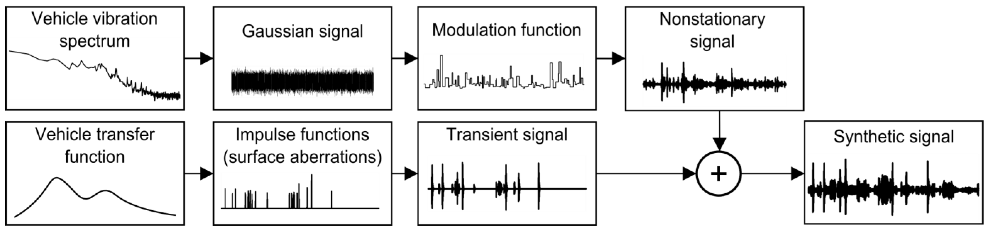
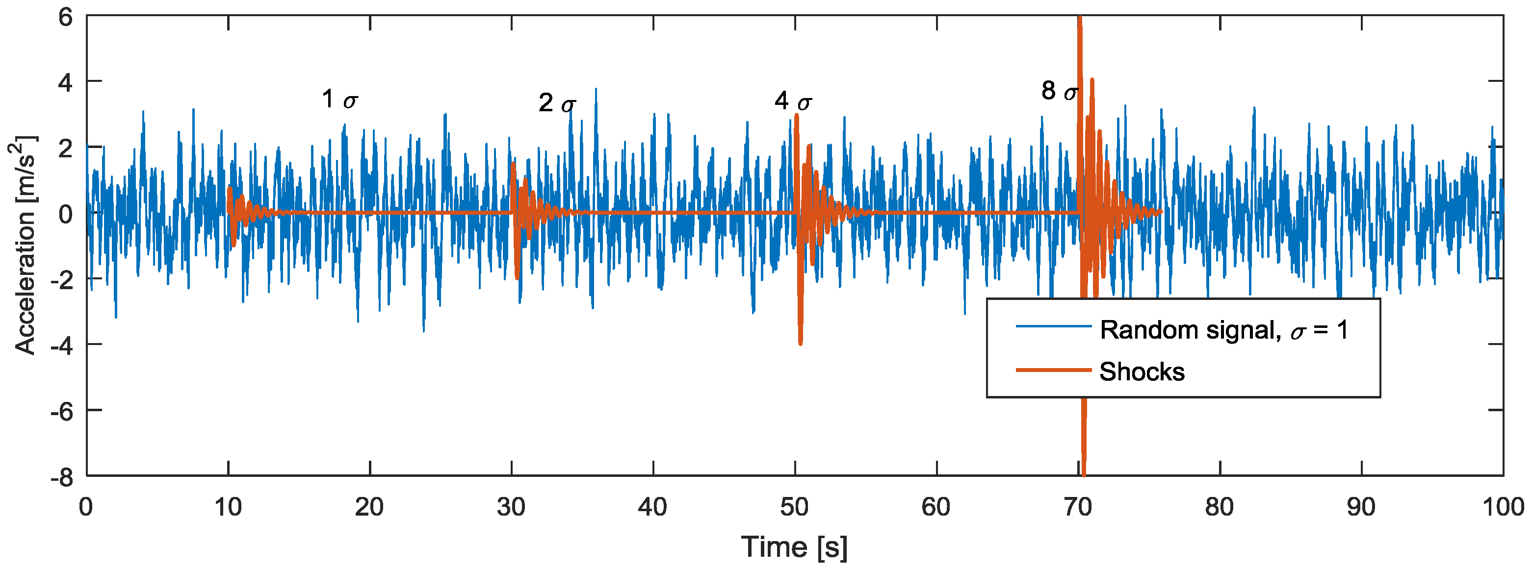
2.2. Synthetic RVV Signals

The algorithm was trained with a synthetic signal (learning dataset) composed of nonstationary random vibrations and shocks, which represented a realistic RVV signal. The advantages of using a synthetic RVV over vibration signals recorded on vehicles are twofold: (1) the signal’s characteristics (such as the location of the shocks) can be precisely known, which is essential to verify the learning process; and (2) the signal can virtually last for any duration of time, which can increase the detection accuracy. To represent the shocks and nonstationarities, the synthesis was made from the sum of two separate signals (Figure 5).

The vehicle vibration spectrum was calculated from vertical acceleration measured on a vehicle. A Gaussian signal was created from an inverse Fast Fourier Transform of the spectrum, modified with a random phase. The nonstationary signal was created from a modulated Gaussian random signal with the spectrum of a typical road vehicle. The modulation function represents typical RMS variations observed in a RVV signal [8,18].

The transient signal is a series of impulse responses of a typical vehicle transfer function. The transfer function corresponds to a two-degree-of-freedom mass-spring-damper model, which represents a quarter-car suspension model of a road transport vehicle [40]. The distribution of the impulse location, duration, and amplitude represented realistic road surface aberrations.

Both the nonstationary and transient signals were added together to create a synthetic RVV signal. Complete details on the RVV signal synthesis are presented by Lepine [35].

Classifiers were trained with a 3000 s dataset (sampling frequency of 1024 Hz), incorporating 300 randomly distributed shocks. The spectrum of RVV signals dropped by several orders above 100 Hz, meaning the sampling frequency was more than 10 times greater than the bandwidth of interest. The classifiers were then validated with a 3500 s dataset (at the same sampling frequency) that contained 350 randomly distributed shocks. Preliminary work from Lepine [35] shows that this combination of both learning and validation datasets is necessary to obtain accurate classification models.

2.3. Predictors

Machine learning prediction performance depends on the data processing undertaken before the training phase—that is, the predictors. In order to detect the shocks buried into RVV signals, the predictors were obtained from the relevant analysis methods, which are: the moving RMS, moving crest factor, moving kurtosis, Hilbert-Huang Transform (HHT), and Discrete Wavelet Transform (DWT). Section 2.3.1, Section 2.3.2, Section 2.3.3, Section 2.3.4 and Section 2.3.5 summarizes the work published by Lepine et al. [30] on the selection and optimization of predictors for RVV shock detection.

2.3.1. Moving RMS

Measuring the fluctuations in the RVV signals’ RMS values gives an overview of their nonstationarities and shocks. The moving RMS with a window duration, T, is defined as:

$$m_{RMS}\left(t\right)=\sqrt{\frac{1}{T}\underset{0}{\overset{T}{{\displaystyle \int }}}x{\left(t+\tau \right)}^{2}d\tau }$$

(4)

where τ is a dummy variable representing a time shift.

Note how the moving RMS is calculated “forward” $\left(t+\tau \right)$ to consider the vehicle causal reaction from the road excitation. The major shortcoming of this predictor indicates its dependency on its window duration. A shorter window is better for detecting short transient events but is ineffective for longer sustained changes in RMS level, and vice versa [16,30], meaning there is no ideal window size. Fortunately, machine learning classification has the capability to use multiple predictors. The moving RMS predictors are not limited to one window length, so two different window lengths (0.5 s and 4 s) are used.

2.3.2. Moving Crest Factor

The moving crest factor is the ratio between the absolute value of the signal over the moving RMS value of a window duration T:

$$m_{CF}\left(t\right)=\frac{\left|x\left(t\right)\right|}{\sqrt{\frac{1}{T}{{\displaystyle \int }}_0^{T}x{\left(t+\tau \right)}^{2}d\tau }}$$

(5)

Note how the moving crest factor is calculated “forward” $\left(t+\tau \right)$ to consider the vehicle causal reaction from the road excitation.

In general, the moving crest factor of a signal increases with the presence of shocks. Therefore, shocks can be detected when the crest factor is above a certain threshold. As opposed to the moving RMS predictor, the moving crest factor predictor is more accurate when using a longer moving window [30]. This is because a longer window averages out the effect of the shock at the crest factor’s denominator without affecting its numerator, which results in a greater sensitivity to shocks. However, windows of too long a duration have been found to misclassify short RMS variations as shocks [30]. Two crest-factor predictors with window lengths of 8 s and 64 s were used to develop the machine learning classifiers.

2.3.3. Moving Kurtosis

The moving kurtosis, κ, is the fourth moment of a signal. It gives a measure of the “peakedness” of the Probability Density Function (PDF) of a signal segment (duration, T) which is defined as:

$$\kappa \left(t\right)=\frac{\frac{1}{T}{{\displaystyle \int }}_0^T{\left[x\left(t+\tau \right)\right]}^{4}d\tau }{{\left(\frac{1}{T}{{\displaystyle \int }}_0^T{\left[x\left(t+\tau \right)\right]}^{2}d\tau \right)}^2}$$

(6)

Two signals with the same RMS value can have different kurtosis if one has a few very high peak values. The kurtosis could also be interpreted as how close a signal’s distribution is to a Gaussian distribution which has a kurtosis of 3. Shocks and nonstationarity components in RVV create a leptokurtic distribution—that is, a kurtosis above 3 [6,19]. Depending on the window length, the moving kurtosis does not have the same sensitivity to signal RMS variations and shocks. Preliminary experiments have shown that by combining two window lengths (4 s and 8 s), the moving kurtosis functions can identify both the shocks and the nonstationarities of RVV [35].

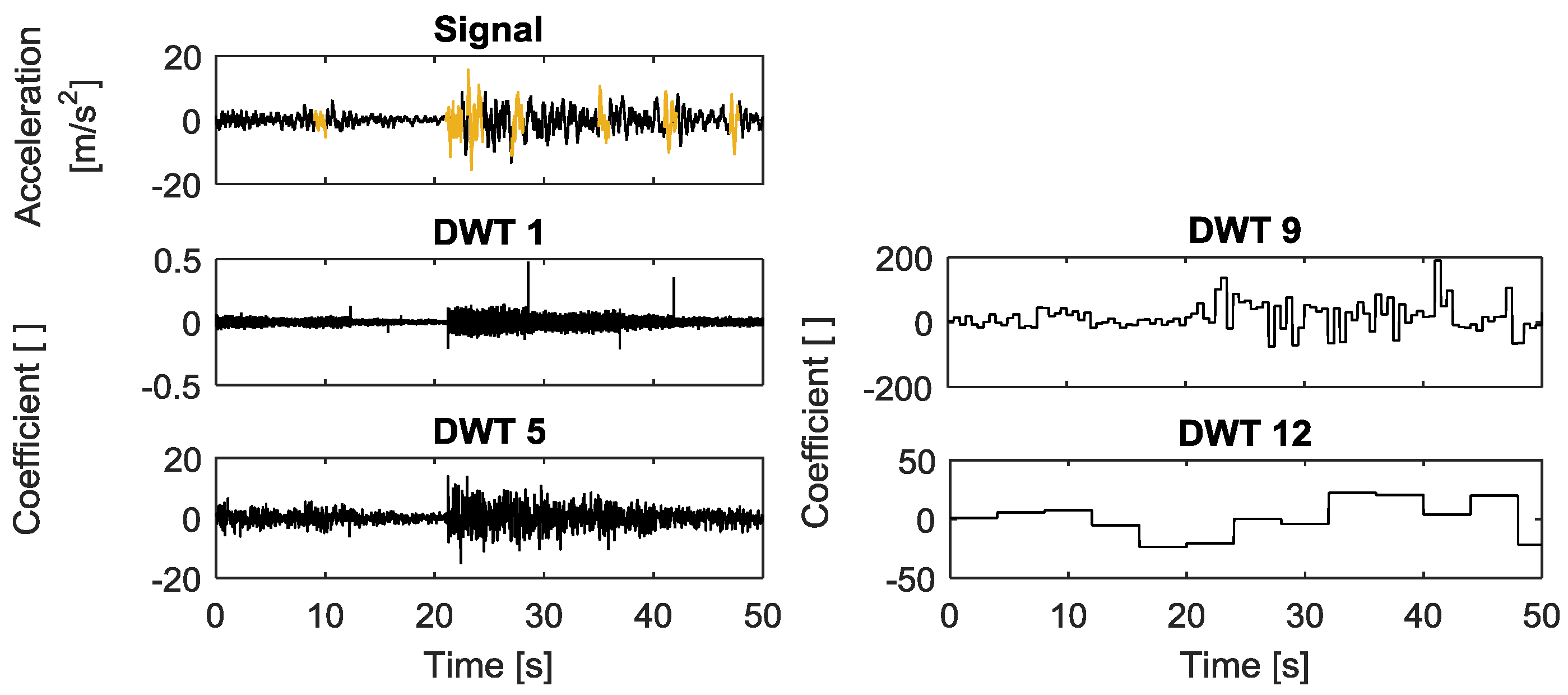
2.3.4. Discrete Wavelet Transform

The DWT is a time-frequency (or more specifically, time-scale) analysis method that provides predictors which are more sensitive to signal changes. Different publications suggest that the Daubechies wavelets are the best suited for RVV analysis [20,21]; thus, the Daubechies 10 wavelet was used to analyse the learning data and coefficients of the first 12 scales, which were directly used as predictors. As the signal sampling rate is halved for every scale, the largest scale (12) has a frequency range up to 0.25 Hz (for a sampling rate of 1024 Hz), which can be considered to be refined enough for RVV analysis purposes. This resampling also causes the number of coefficients to decrease at every scale. To create predictors with sampling rates that match the original signal and the other predictors, the coefficients are replicated to match the sampling rate of the signal. Figure 6 presents an example of the DWT predictors of four different scales of the signal.

A full description of the specific application of the DWT, including its mathematical derivation, can be found in previous publications [22,30,35].

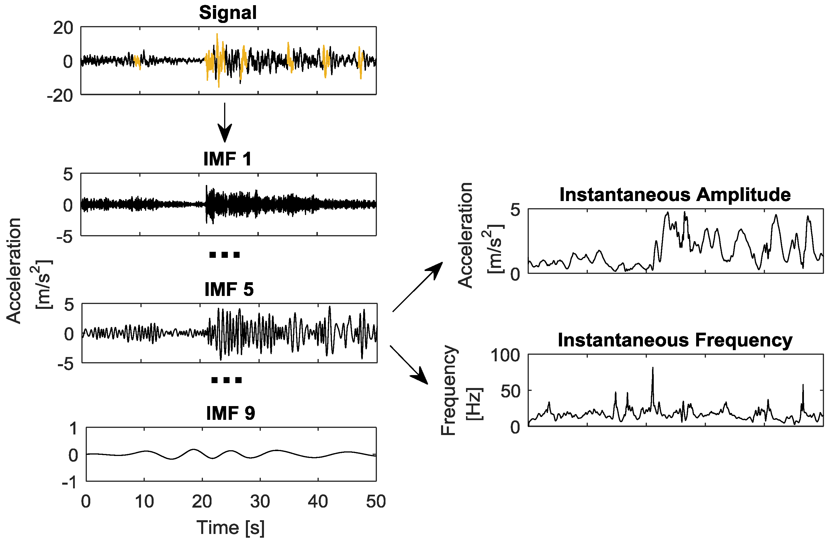
2.3.5. Hilbert-Huang Transform Predictors

The Hilbert-Huang Transform (HHT) is an adaptive time-frequency analysis method providing different types of predictors from RVV signals. The HHT uses a sifting process to decompose a signal into different narrow-banded components called Intrinsic Mode Functions (IMFs), which have the following characteristics, as defined by Huang et al. [34]:

• In the whole dataset, the number of extrema and number of zero-crossings must either be equal to each other, or differ by one at most;
• At any point, the mean value of the envelopes defined by the local maxima and local minima is zero.

The sifting process is made by fitting a spline function over signal local maxima and a second over local minima. The mean of these functions is then subtracted from the signal, which has the effect of removing the low-frequency components of the signal. This process is repeated until the number of extrema and zero-crossings remain the same and either equal to each other, or differ, at most, by one, for eight consecutive iterations [41]; the remaining signal becomes the first IMF. The next IMFs are then calculated using what remains from the signal, using the same process. This iterative process stops when no more IMF can be fitted, and the residual is called the signal trend. The predictors used in the machine learning process are the instantaneous amplitude and frequency functions of each IMF, which can be calculated using the Hilbert transform. These functions reveal trend changes in the signal, which make them effective predictors. For example, Figure 7 shows IMFs 1, 5, and 9 of a signal, along with IMF 5’s instantaneous amplitude envelope and instantaneous frequency functions.

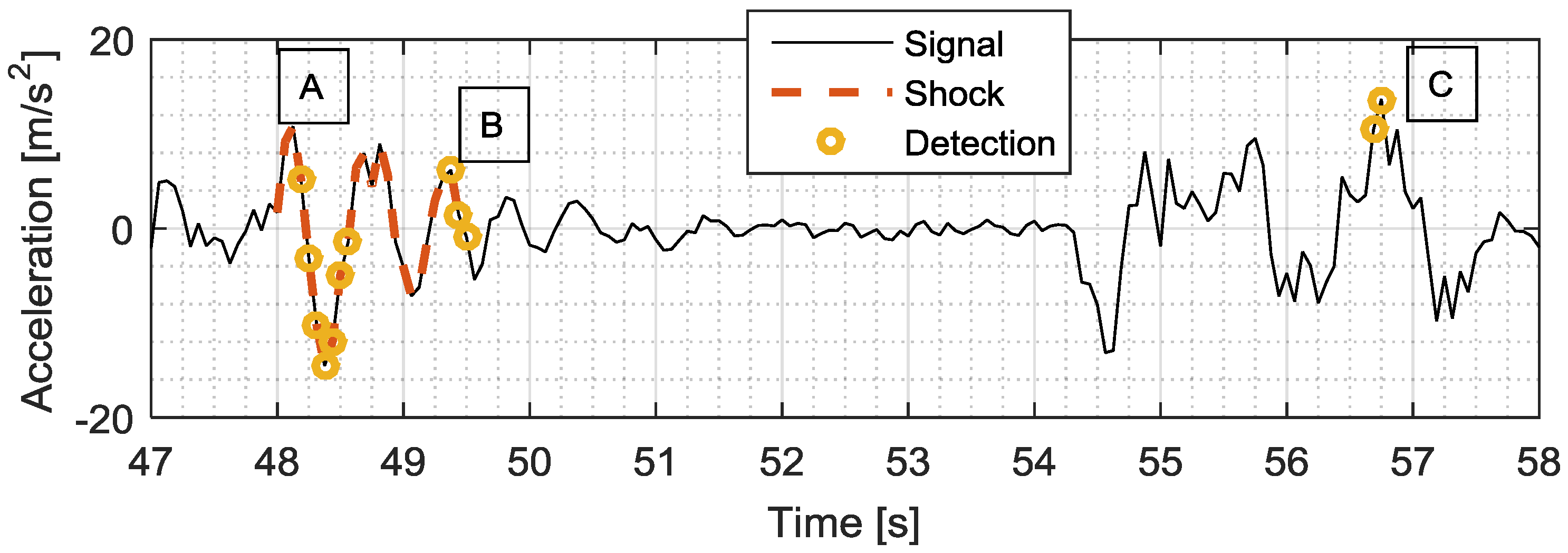
2.3.6. Detection Enhancement Algorithm

The detections made by the selected classifiers are discrete and independent of the predictors’ order. In other words, a classification at one time is not affected by and does not affect previous and future classifications. Therefore, the causality of the shock responses is only considered in the predictor computations and not in the classification algorithms. This means that the shock detections can be scattered, rather than continuous. For instance, the shock buried in the signal in Figure 8 between 48 s and 48.5 s can be detected in two distinct segments. These incomplete detections decrease the classifier’s accuracy.

An algorithm was specially developed to enhance the continuity of the detections for RVV analysis and shock detection. The detection enhancement algorithm extends the detection sequences to ensure they have at least the same duration as the longest impulse response function (in this specific case, 1.4 s) which is the period of the first natural frequency of the vehicle shock response. This is more than the period of the natural frequency of the two-degree-of-freedom vehicle model used to synthesize the signal.

The algorithm is an iterative process, described in Figure 9. It starts at the detection point with the maximum absolute value of the signal, and then creates a 1.4 s window which corresponds to approximately 2.5 times the period of the first natural frequency of the vehicle transfer function used in the model synthesis. The starting point of the window is positioned 0.28 s before the absolute maximum. This places the absolute maximum at 20% of the window length, which places the window at approximately the beginning of the vehicle shock response. The algorithm interprets all the data points in this window as a shock if at least 10% of these data points were classified as shock by the classifier, as shown in Figure 9a,b. In this case, the window points and the continuous detections adjacent to it are considered as a shock segment. This 10% overlap criterion is based on an arbitrary value which only affects the classifier’s operating point threshold (see next section). If the 10% detection overlap criterion is negative, the window is classified as no-shock, and the detection points made by the classifier are voided, as shown at Figure 9b,c; this concludes the first iteration. The algorithm continues this iterative process by finding the next maximum absolute detection acceleration, excluding the points from the segment created in the previous iterations. The windowing process is then performed, and the 10% detection overlap criterion is applied using all the data points, including those from the previous iterations.

3. Classifier Evaluation

Classifier validation is an essential step in machine learning; it assesses the detection accuracy and calibrates the detection sensitivity of the algorithm. Depending on the application, different criteria can be used to evaluate detection performances. The following sections show that classical evaluation methods are not ideally suited to validation and calibration of the shock detection algorithm, creating the need to develop more specific evaluation methods.

3.1. Classical Detection Assessment

Classifiers base their prediction on a sufficient statistic which is calculated from predictors. The sufficient statistic is compared to a threshold value to attribute a class to a data point. This can be seen as the probability that a data point belongs to one class over another. For various reasons, the classification is not necessarily made when there is more than a 50% chance that a data point is from a specific class—other probabilities or threshold values are often used. Changing this threshold varies the amount of true detections, misdetections, and false detections, which can be assessed in terms of sensitivity and specificity.

In this context, the usual definition of sensitivity is the proportion of shock data points in the signal that are correctly classified as such. However, for the purposes of RVV signal analysis, sensitivity can be assessed using a modified definition. The shocks can be considered as a sequence of data points instead of individual data points. Considering this, the definition of sensitivity becomes the number of true detection sequences over the total number of shocks.

$$\mathrm{S}ensitivity=\frac{\mathrm{Number}\mathrm{of}\mathrm{True}\mathrm{Detections}}{\mathrm{Number}\mathrm{of}\mathrm{Shocks}}$$

(7)

where a detection has to overlap at least 75% of the shock duration to be considered true. This 75% overlap is an arbitrary value, ensuring that an significant proportion of the shock is detected.

Converse to sensitivity, the specificity is the proportion of the signal without shock that is correctly classified as such. This can be considered as the accuracy of the prediction of the duration of the signal without shock. The definition of the specificity is not modified, and is considered to be the number of true nondetection data points over the number of data points without transients.

$$\mathrm{S}pecificity=\frac{\mathrm{Number}\mathrm{of}\mathrm{Nondetection}\mathrm{Data}\mathrm{Points}}{\mathrm{Number}\mathrm{of}\mathrm{Data}\mathrm{Points}\mathrm{without}\mathrm{Shocks}}$$

(8)

The sensitivity and specificity are specific to the operating point—that is, the threshold value used for the detection. Using a low detection threshold increases the sensitivity to the detriment of the specificity, and vice versa. This relationship is represented by the ROC (Receiver Operating Characteristic) curve, which displays the sensitivity as a function of the fall-out (i.e., probability of a false detection, which is equal to 1—specificity). A simple method which can be used to assess and compare classifiers’ performance is to calculate the area under the ROC curve (AUC) [42,43]. The ideal classifier has an AUC of 1, and a classifier based on chance has an area of 0.5. This means that a classifier with an AUC above 0.5 has better prediction performance than chance.

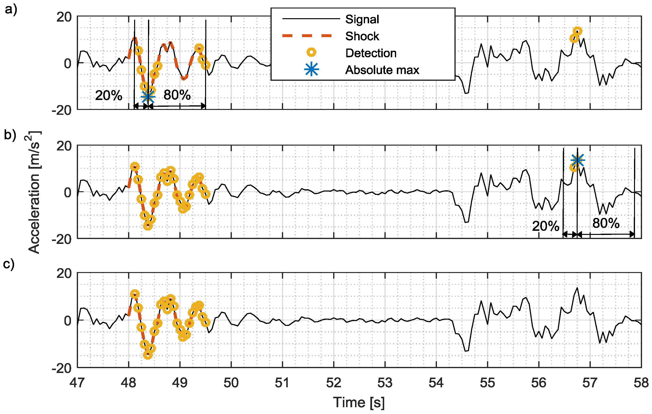
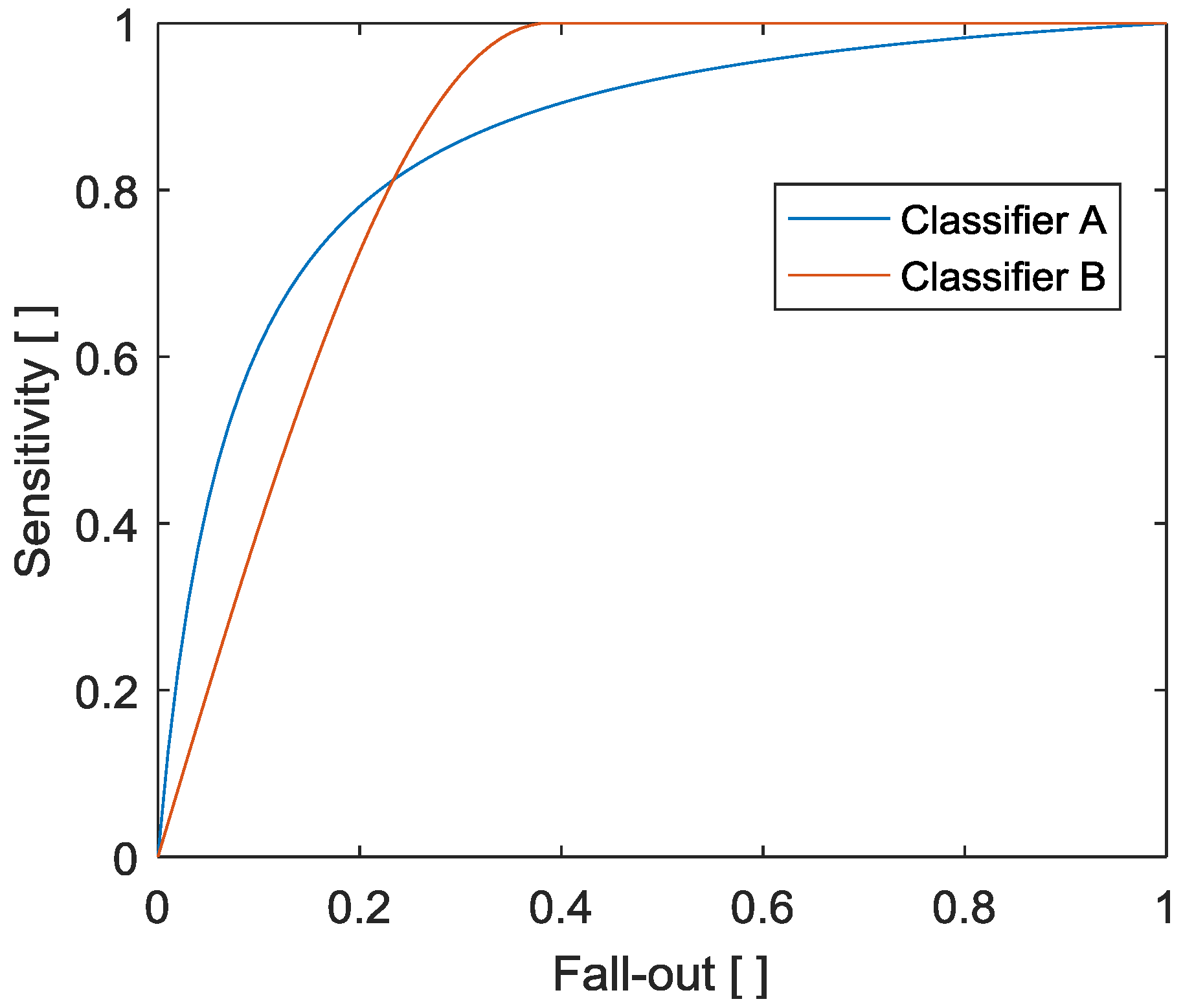
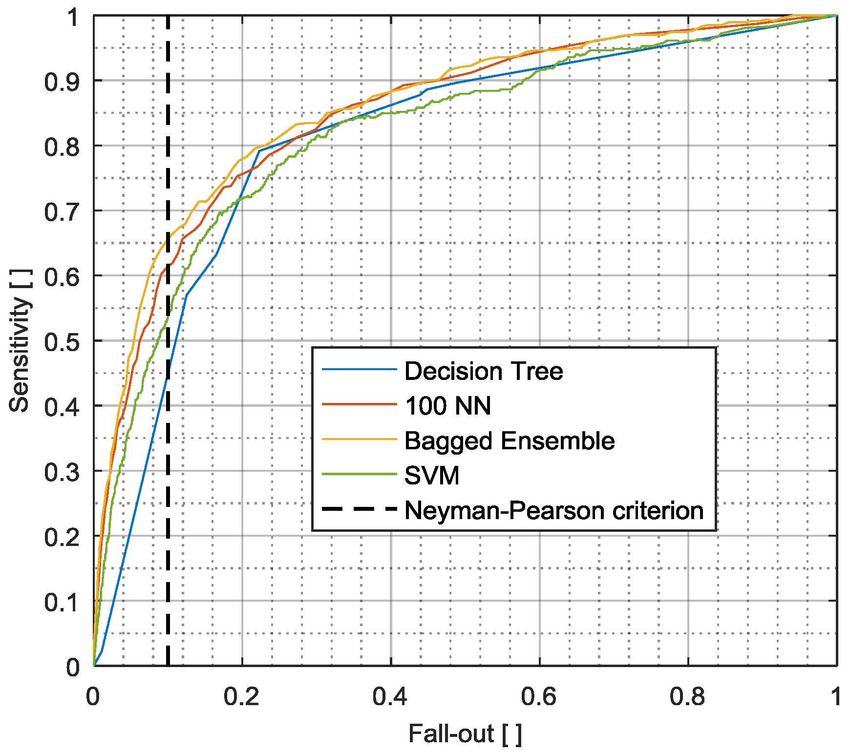
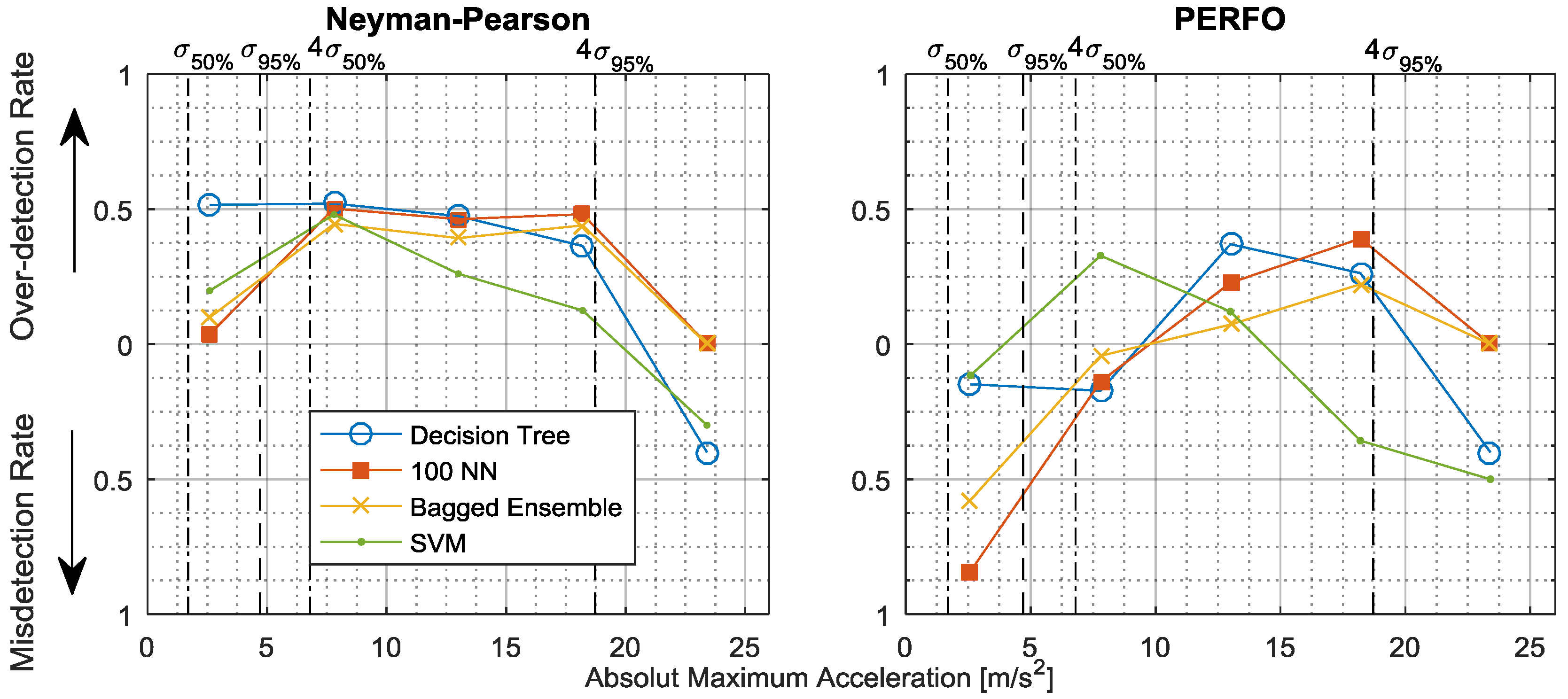
3.1.1. Optimal Operation Point

The AUC value is a convenient accuracy measurand because it integrates both the classifier sensitivity and specificity dependence in a single value. However, this simplicity is also a significant shortcoming, because it can lead to false comparisons [44]. The AUC gives the ROC’s global performance but does not account for its shape or any local features. For instance, two classifiers can have the same AUC but significantly different ROC shapes, as shown in Figure 10. Classifier A has better sensitivity at a low fall-out value, but reaches a 100% detection rate almost at 100% fall-out. On the other hand, classifier B has poor sensitivity at low fall-out, but surpasses classifier A’s sensitivity for any fall-out value over 0.23. Thus, classifier A is better for an application where a low false-detection rate is required, and classifier B is better for an application where a higher detection rate is more important, regardless of false detections.

This leads to an important concept in detection theory: the optimal operation point (OOP). Classifiers give the probability that a class exists. However, even if the probability is more than 50%, it does not necessarily mean than this class should be considered detected. One could assume that 1% fall-out is very good, but not if it is used to detect very unlikely events, as 1% of samples will be false positive. It is therefore imperative to find the optimal trade-off between the fall-out and the sensitivity for a specific classifier and application. This trade-off is known as the OOP, and can be found on the ROC curve using the Neyman-Pearson criterion.

The Neyman-Pearson criterion finds the OOP without knowing the a priori probability and without attributing any decision cost [45], which is the case for RVV shock detection. This criterion is fairly simple; it determines the OOP by fixing the fall-out to a certain level, and by using the point where the ROC curve crosses this level. Limiting the maximum level of false detection (fall-out) can be seen as fixing the significance level of the detection. For example, for a 10% significance level or fall-out, the operation point on the ROC is where the fall-out equals to 0.1, as presented at Figure 11.

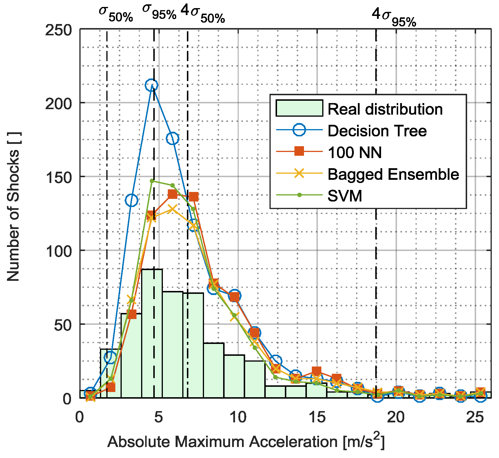
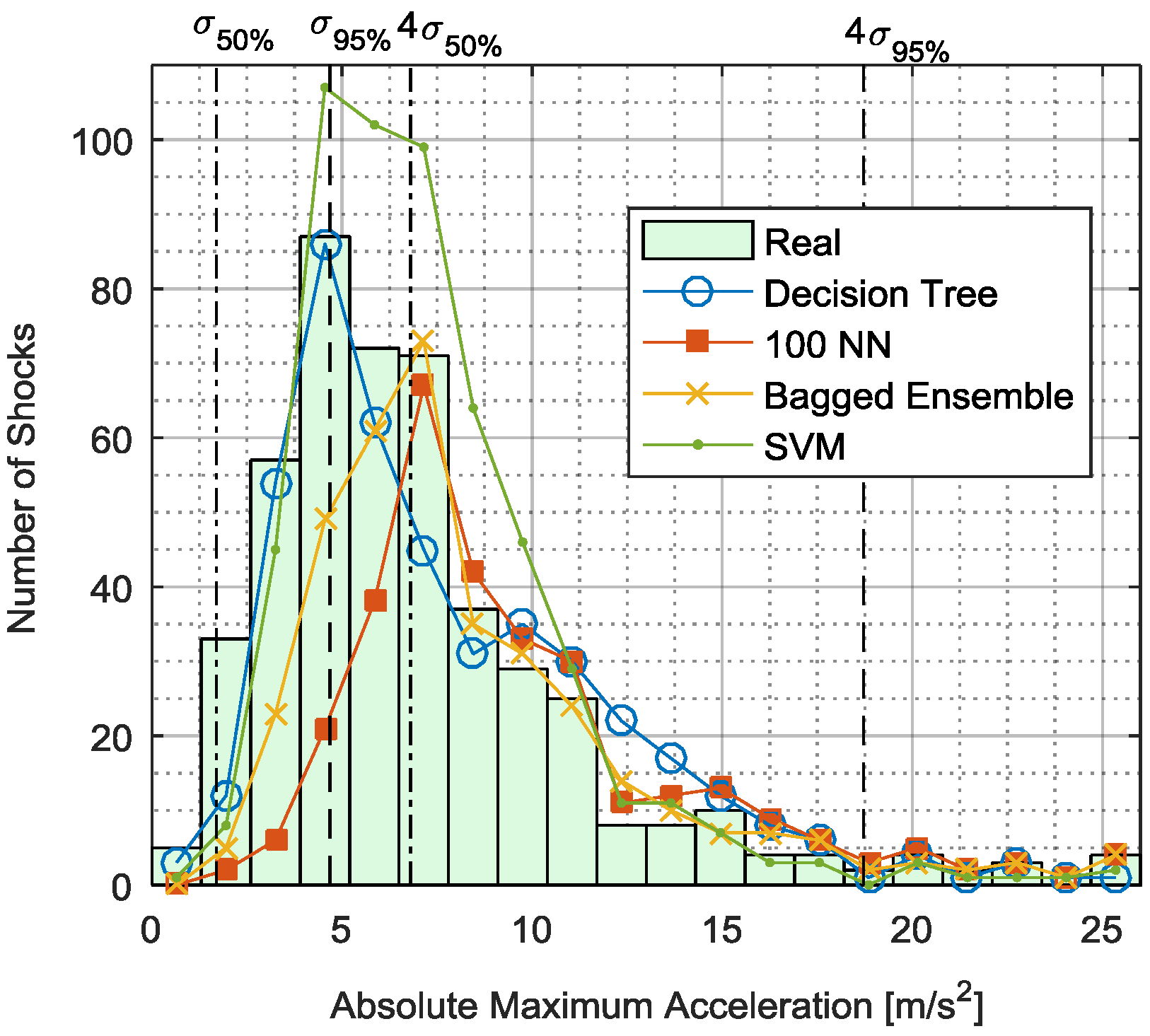
3.1.2. Neyman-Pearson Maximum Amplitude Distribution

The ROC curve and OOP coordinates give a good indication of the true and false detection rates of the classifiers; however, they do not provide any insight into the quality of their detections. RVV simulation accuracy depends on the characteristics of each of its modes. As previously explained, once the shocks are detected in a RVV signal, they can be extracted independently. The other modes can then be separately characterized in the remaining signal without their parameters being affected by the shocks.

The main parameter used to characterize shocks was the maximum absolute amplitude which defines the severity of the shocks. The classifiers’ detection quality can be assessed by comparing the maximum absolute acceleration distributions for the real shocks and the detections (true and false detections) using the OOP defined by the Neyman-Pearson criterion (Figure 12). These distributions represent the maximum absolute acceleration values of each shock superimposed on the signal (real distribution) and each shock detection (detection distribution). Comparing the real and the detected shock-amplitude distributions gives more insight about the classifiers’ detection quality than the sensitivity and fall-out values, because it indicates which shock intensities are more likely to be misclassified. The RMS value of the signal is shown in Figure 12 to give an indication of relative shock intensities.

The significance of the shock amplitude is relative to the intensity of the signal. As presented in Figure 13, shocks with a maximum absolute amplitude which are inferior to four times the RMS value (standard deviation, σ, for zero mean signals) of the underlying random Gaussian signal are barely noticeable and have little effect on RVV. As RVV are nonstationary signals, the intensity cannot be assessed with a single RMS value, but can be assessed with the distribution RMS value of the stationary Gaussian random segments which compose of the signal. In order to visualize the relative importance of the shocks buried in the RVV signal, the median, σ_50%, and the 95th percentile, σ_95%, RMS values and four times their respective values, 4σ_50% and 4σ_95%, are presented on the shock amplitude distribution and misdetection/over-detection plots.

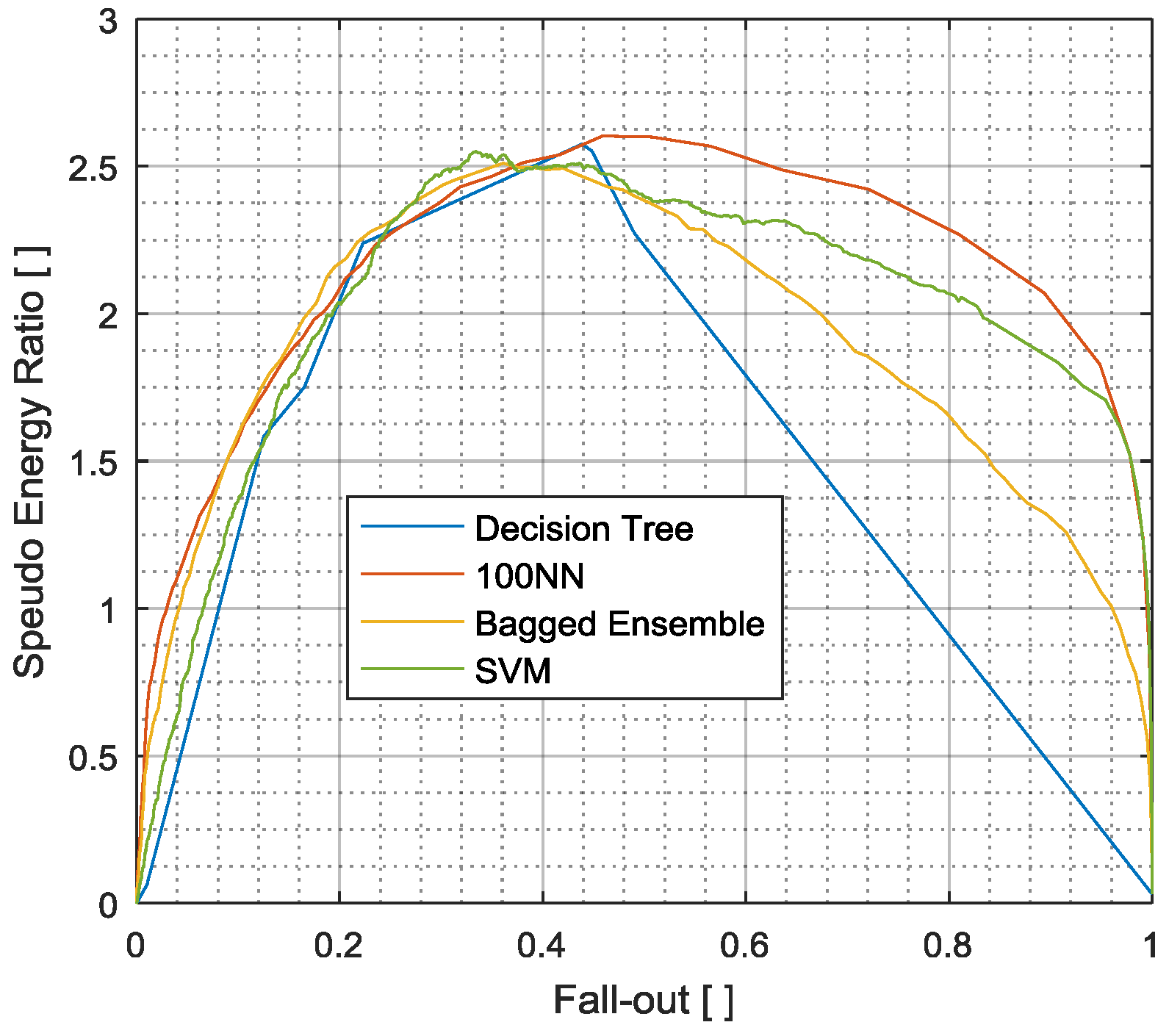
3.2. Pseudo-Energy Ratio/Fall-Out (PERFO) Curve

A comparison of the distribution of the maximum absolute accelerations of the real shocks and detections reveals much detail on the classifiers’ accuracy and detection quality. However, this is not a convenient approach, as the distribution comparison is qualitative, rather than quantitative. To improve this, the detections’ maximum absolute acceleration correctness can be reduced to a single number.

Since the importance of detecting shocks increases with their amplitude, the classifiers’ accuracy and quality can be assessed as being the ratio between the detection and the shocks’ maximum absolute acceleration pseudo-energy, calculated as:

$$R=\frac{\sum {\left[\mathrm{Detections}’\mathrm{Max}\mathrm{Absolute}\mathrm{Acceleration}\right]}^2}{\sum {\left[\mathrm{Shocks}’\mathrm{Max}\mathrm{Absolute}\mathrm{Acceleration}\right]}^2}$$

(9)

As for sensitivity, the pseudo-energy ratio depends on the classifier’s detection threshold and directly affects the fall-out level. The relationship between the pseudo-energy ratio and the fall-out is presented in Figure 14. Contrary to the ROC curve, the Pseudo-Energy Ratio/Fall-Out (PERFO) curve does not end at the coordinate (1, 1) and is not monotonic. This is because reducing the detection threshold increases the length of signal segments considered as shocks. As the segments become longer, they may include more than one shock. However, only the absolute acceleration of each segment is considered in the PERFO calculation, such that only the shock with the highest amplitude is assessed. Therefore, the larger the detection segments become, the more shocks are potentially left out of this analysis, which explains why the pseudo-energy ratio drops after a certain point. It can be seen in Figure 14 that this drop appears for fall-out from between 0.3 and 0.5, depending on the classifier. As the classifiers operate under this fall-out level, it does not affect the current analysis.

The detection quality can be assessed by observing where the PERFO curve has a pseudo-energy ratio of one, which represents the operation point where the pseudo-energy of the detection and the actual shocks in the signal are equal. Since the pseudo-energy is calculated from the maximum squared absolute amplitude, the lower the fall-out value is at this point, the fewer high-amplitude false detections are present in the classification. Hence, the PERFO curve measures how accurately the correct amount of pseudo-shock energy is detected in a signal.

PERFO Maximum Amplitude Distribution

The PERFO criterion is designed to give a more accurate maximum amplitude detection distribution than the “classical” OOP criteria. This improvement can be observed in Figure 15, where the detection distribution of each classifier follows the real shock distribution more closely when compared to the results shown in Figure 12.

3.3. Comparison of Evaluation Measurands

Three evaluation measurands were presented to validate and calibrate the RVV shock classifiers. The AUC gives a global appreciation of the classifiers’ performances; the greater the AUC, the more predictive power the classifier has, and a value of 0.5 is equivalent to guessing the signal class. The limitation of this measurand is its independence to the detection threshold. To overcome this, the position of the OOP on the ROC curve can be used as an evaluation measurand. The classifiers’ sensitivity at 10% fall-out (Neyman-Pearson criterion) gives a more specific evaluation for the application. The quality of the detection can also be used to refine the position of the OOP, using the PERFO curve. The advantage of the PERFO criterion is that it ensures the detection has the same peak-value pseudo-energy than the shocks present in the signal. A low fall-out value at a pseudo-energy ratio of one on the PERFO curve indicates that there was only a small number of false detections. The results of each evaluation measurand is given in

Table 1. Comparison of classifier evaluation measurands, such as: the AUC; the resulting Neyman-Pearson OOP sensitivity for a 10% fall-out; and the resulting PERFO criterion OOP fall-out.

Classifier	AUC	Neyman-Pearson	PERFO
Decision Tree	0.81	0.45	0.08
100NN	0.85	0.61	0.03
Bagged Ensemble	0.86	0.65	0.04
SVM	0.82	0.54	0.07

.

According to the AUC and the Neyman-Pearson criterion, the Bagged Ensemble is a more accurate classifier, followed by the 100NN. The PERFO criterion, however, ranked the 100NN first, and the Bagged Ensemble second. The ranking of the SVM and Decision Tree remained third and fourth, respectively, with all the measurands.

For shock-detection applications, the PERFO ranking is more accurate as it defines a more relevant OOP. This can be observed by comparing the maximum amplitude distributions for detection made at both OOPs (Figure 12 for Neyman-Pearson, and Figure 15 for PERFO). The shape of the distributions makes the analysis of the high-acceleration region difficult, such as where it matters the most. This is because the number of high-amplitude shocks is too small in comparison to the total amount of shocks, and the discrepancies within the classifiers’ distribution cannot be easily seen in that region. To facilitate the comparison, the error between the detection and the real distributions were presented on the misdetection/over-detection graphs (Figure 16). These graphs show the average difference between the number of detections and the real shocks distributed into five bins. When a bin has more detections than real shocks, the over-detection rate is calculated by dividing the difference by the number of detections. On the other hand, when a bin has more shocks than detections, the misdetection rate is calculated by dividing the difference by the number of real shocks. Lower values for both the over-detection and misdetection rate indicate better classification performance.

As seen in Figure 16, the Neyman-Pearson OOP over-detected below 4σ_95% (≈19 m/s^s) for all the classifiers. Above 4σ_95%, this OOP made for perfect detection (0 over-detection and misdetection rates) for the 100NN and the Bagged Ensemble algorithms. The Decision Tree and SVM algorithms misdetected 40% and 30% of the shocks, respectively. For most of the classifiers, the PERFO criterion defined a better OOP. For low-amplitude shocks (below ≈ 2σ_95% or 10 m/s^s), the classifiers misdetected shocks rather than over-detecting them, as with the Neyman-Pearson. Above this amplitude, most of the PERFO distribution errors improved, and the Decision Tree, 100NN, and Bagged Ensemble had lower misdetection and over-detection rates. Only the SVM detected less shocks (for both low- and high-amplitude) with the PERFO criterion than with the Neyman-Pearson criterion.

4. Summary of Discussion

The Neyman-Pearson criterion effectively defines classifiers’ OOP when all the detections have the same importance. However, for applications such as the detection of shocks buried in RVV signals, especially for protective packaging optimization, not all shocks have the same importance, as high-amplitude shocks create more damage to freight. For this application, the PERFO criterion gave a more appropriate OOP, ensuring that the detection amplitude distribution followed the shock amplitude distribution more closely. For the four selected classifiers, the PERFO criterion reduced the over-detection rate, especially for low-amplitude shocks, without compromising the high-amplitude detection (except for the SVM showing a high misdetection rate with the PERFO criterion).

For protective packaging optimization purposes, this means that a simulation performed with the PERFO detection would have a more accurate relative proportion of low- and high-amplitude shocks. Considering that significant shocks have maximum amplitude above 4σ_95%, the Bagged Ensemble classification algorithm seems best-suited for the application as it has the best performance above this value (Figure 16). This conclusion should, however, be validated with real vehicle data.

The classification algorithms are based on many parameters, such as the number of tests for the Decision Tree or the type of distance and number of nearest neighbors for the kNN. Classifiers’ parameters can be optimized using the PERFO OOP fall-out. An optimization based on this single value ensures that classifiers provide their best shock-detection performance.

The PERFO curve and criterion can also be adapted to other classification applications where not all detections/misdetections have the same importance, e.g., structural damage detection on a structure, or economic fraud detection. Depending on the application, the square exponent in the pseudo-energy calculation can be replaced by another exponent, which will modulate the importance of high-value detection.

5. Conclusions

This paper has shown that machine learning classification algorithms can be used to detect shocks present in RVV signals. The performance of different algorithms (Decision Tree, 100NN, Bagged Ensemble, and SVM) were assessed using various methods. Considering that high-amplitude shocks are more important, the PERFO curve and the resulting OOP were shown to be better performance indicators than the classic assessment tools, such as the area under the ROC curve (AUC) and the Neyman-Pearson OOP sensitivity, because they give an appreciation of the detection quality.

References

1. ASTM International. Test Method for Random Vibration Testing of Shipping Containers; ASTM-D4728; ASTM International: West Conshohocken, PA, USA, 2012. [Google Scholar]
2. Department of Defense Test Method Standard. Environmental Test Methods and Engineering Guides; MIL-STD-810F; Department of Defense Test Method Standard: Columbus, OH, USA, 2000. [Google Scholar]
3. BSI. Packaging. Complete, Filled Transport Packages and Unit Loads. Vertical Random Vibration Test; ISO-13355; BSI: London, UK, 2002; p. 16. [Google Scholar]
4. ISTA. Test Series. Available online: https://www.ista.org/pages/procedures/ista-procedures.php (accessed on 5 October 2016).
5. Charles, D. Derivation of Environment Descriptions and Test Severities from Measured Road Transportation Data. J. IES 1993, 36, 37–42. [Google Scholar]
6. Rouillard, V. On the Synthesis of Non-Gaussian Road Vehicle Vibrations. Ph.D. Thesis, Monash University, Melbourn, Australia, 2007. [Google Scholar]
7. Kipp, W.I. Random Vibration Testing of Packaged-Products: Considerations for Methodology Improvement. In Proceedings of the 16th IAPRI World Conference on Packaging, Bangkok, Thailand, 8–12 June 2008. [Google Scholar]
8. Rouillard, V.; Sek, M. Creating Transport Vibration Simulation Profiles from Vehicle and Road Characteristics. Packag. Technol. Sci. 2013, 26, 82–95. [Google Scholar] [CrossRef]
9. Rouillard, V. Generating Road Vibration Test Schedules from Pavement Profiles for Packaging Optimization. Packag. Technol. Sci. 2008, 21, 501–514. [Google Scholar] [CrossRef]
10. Rouillard, V.; Bruscella, B.; Sek, M. Classification of road surface profiles. J. Transp. Eng. 2000, 126, 41–45. [Google Scholar] [CrossRef]
11. Bruscella, B.; Rouillard, V.; Sek, M. Analysis of road surface profiles. J. Transp. Eng. 1999, 125, 55–59. [Google Scholar] [CrossRef]
12. Bruscella, B. The Analysis and Simulation of the Spectral and Statistical Properties of Road Roughness for Package Performance Testing; Department of Mechanical Engineering, Victoria University of Technology: Melbourne, Australia, 1997. [Google Scholar]
13. Garcia-Romeu-Martinez, M.-A.; Rouillard, V.; Cloquell-Ballester, V.-A. A Model for the Statistical Distribution of Road Vehicle Vibrations. In World Congress on Engineering 2007: WCE 2007; Imperial College London: London, UK, 2007; pp. 1225–1230. [Google Scholar]
14. Garcia-Romeu-Martinez, M.-A.; Singh, S.P.; Cloquell-Ballester, V.-A. Measurement and analysis of vibration levels for truck transport in Spain as a function of payload, suspension and speed. Packag. Technol. Sci. 2008, 21, 439–451. [Google Scholar] [CrossRef]
15. Rouillard, V.; Sek, M.A. A statistical model for longitudinal road topography. Road Transp. Res. 2002, 11, 17–23. [Google Scholar]
16. Rouillard, V. Quantifying the Non-stationarity of Vehicle Vibrations with the Run Test. Packag. Technol. Sci. 2014, 27, 203–219. [Google Scholar] [CrossRef]
17. Rouillard, V.; Sek, M.A. Monitoring and simulating non-stationary vibrations for package optimization. Packag. Technol. Sci. 2000, 13, 149–156. [Google Scholar] [CrossRef]
18. Rouillard, V.; Sek, M.A. Synthesizing Nonstationary, Non-Gaussian Random Vibrations. Packag. Technol. Sci. 2010, 23, 423–439. [Google Scholar] [CrossRef]
19. Steinwolf, A.; Connon, W.H., III. Limitations of the Fourier transform for describing test course profiles. Sound Vib. 2005, 39, 12–17. [Google Scholar]
20. Wei, L.; Fwa, T.; Zhe, Z. Wavelet analysis and interpretation of road roughness. J. Transp. Eng. Asce 2005, 131, 120–130. [Google Scholar] [CrossRef]
21. Nei, D.; Nakamura, N.; Roy, P.; Orikasa, T.; Ishikawa, Y.; Kitazawa, H.; Shiina, T. Wavelet analysis of shock and vibration on the truck bed. Packag. Technol. Sci. 2008, 21, 491–499. [Google Scholar] [CrossRef]
22. Lepine, J.; Rouillard, V.; Sek, M. Wavelet Transform to Index Road Vehicle Vibration Mixed Mode Signals. In Proceedings of the ASME 2015 Noise Control and Acoustics Division Conference at InterNoise 2015, San Francisco, CA, USA, 9–12 August 2015. [Google Scholar]
23. Ayenu-Prah, A.; Attoh-Okine, N. Comparative study of Hilbert–Huang transform, Fourier transform and wavelet transform in pavement profile analysis. Veh. Syst. Dyn. 2009, 47, 437–456. [Google Scholar] [CrossRef]
24. Griffiths, K.R. An Improved Method for Simulation of Vehicle Vibration Using a Journey Database and Wavelet Analysis for the Pre-Distribution Testing of Packaging. Ph.D. Thesis, University of Bath, Bath, UK, 2012. [Google Scholar]
25. Lepine, J.; Rouillard, V.; Sek, M. Using the Hilbert-Huang transform to identify harmonics and transients within random signals. In Proceedings of the 8th Australasian Congress on Applied Mechanics: ACAM 8, Melbourne, Australia, 25–26 November 2014. [Google Scholar]
26. Mao, C.; Jiang, Y.; Wang, D.; Chen, X.; Tao, J. Modeling and simulation of non-stationary vehicle vibration signals based on Hilbert spectrum. Mech. Syst. Signal Process. 2015, 50, 56–69. [Google Scholar] [CrossRef]
27. Lepine, J.; Sek, M.; Rouillard, V. Mixed-Mode Signal Detection of Road Vehicle Vibration Using Hilbert-Huang Transform. In Proceedings of the ASME 2015 Noise Control and Acoustics Division Conference at InterNoise 2015, San Francisco, CA, USA, 9–12 August 2015. [Google Scholar]
28. Lepine, J.; Rouillard, V.; Sek, M. Evaluation of machine learning algorithms for detection of road induced shocks buried in vehicle vibration signals. Proc. Inst. Mech. Eng. Part D J. Automob. Eng. 2018. [Google Scholar] [CrossRef]
29. Rouillard, V.; Lamb, M. On the Effects of Sampling Parameters When Surveying Distribution Vibrations. Packag. Technol. Sci. 2008, 21, 467–477. [Google Scholar] [CrossRef]
30. Lepine, J.; Rouillard, V.; Sek, M. On the Use of Machine Learning to Detect Shocks in Road Vehicle Vibration Signals. Packag. Technol. Sci. 2016, 30, 387–398. [Google Scholar] [CrossRef]
31. Chonhenchob, V.; Singh, S.P.; Singh, J.J.; Stallings, J.; Grewal, G. Measurement and Analysis of Vehicle Vibration for Delivering Packages in Small-Sized and Medium-Sized Trucks and Automobiles. Packag. Technol. Sci. 2012, 25, 31–38. [Google Scholar] [CrossRef]
32. Wallin, B. Developing a Random Vibration Profile Standard; International Safe Transit Association: East Lansing, MI, USA, 2007. [Google Scholar]
33. Rouillard, V.; Richmond, R. A novel approach to analysing and simulating railcar shock and vibrations. Packag. Technol. Sci. 2007, 20, 17–26. [Google Scholar] [CrossRef]
34. Huang, N.E.; Shen, Z.; Long, S.R.; Wu, M.C.; Shih, H.H.; Zheng, Q.; Yen, N.-C.; Tung, C.C.; Liu, H.H. The empirical mode decomposition and the Hilbert spectrum for nonlinear and non-stationary time series analysis. Proc. R. Soc. Lond. Ser. A Math. Phys. Eng. Sci. 1998, 454, 903–995. [Google Scholar] [CrossRef]
35. Lepine, J. An Optimised Machine Learning Algorithm for Detecting Shocks in Road Vehicle Vibration. Ph.D. Thesis, College of Engineering and Science, Victoria University, Melbourne, Australia, 2016. [Google Scholar]
36. Hastie, T.; Tibshirani, R.; Friedman, J.; Franklin, J. The Elements of Statistical Learning: Data Mining, Inference and Prediction; Springer: New York, NY, USA, 2005; Volume 27. [Google Scholar]
37. Rogers, S.; Girolami, M. A First Course in Machine Learning; CRC Press: Boca Raton, FL, USA, 2011. [Google Scholar]
38. Cherkassky, V.; Mulier, F.M. Learning from Data: Concepts, Theory, and Methods; John Wiley & Sons: Hoboken, NJ, USA, 2007. [Google Scholar]
39. Shalev-Shwartz, S.; Ben-David, S. Understanding Machine Learning: From Theory to Algorithms; Cambridge University Press: Cambridge, UK, 2014. [Google Scholar]
40. Cebon, D. Handbook of Vehicle-Road Interaction/David Cebon: Lisse; Swets & Zeitlinger: Abingdon, UK, 1999. [Google Scholar]
41. Huang, N.E.; Wu, M.-L.C.; Long, S.R.; Shen, S.S.; Qu, W.; Gloersen, P.; Fan, K.L. A confidence limit for the empirical mode decomposition and Hilbert spectral analysis. Proc. R. Soc. Lond. Ser. A Math. Phys. Eng. Sci. 2003, 459, 2317–2345. [Google Scholar] [CrossRef]
42. Bradley, A.P. The use of the area under the ROC curve in the evaluation of machine learning algorithms. Pattern Recogn. 1997, 30, 1145–1159. [Google Scholar] [CrossRef] [Green Version]
43. Ling, C.X.; Huang, J.; Zhang, H. AUC: A better measure than accuracy in comparing learning algorithms. In Advances in Artificial Intelligence; Springer: Berlin, Germany, 2003; pp. 329–341. [Google Scholar]
44. Powers, D.M.W. The problem of Area Under the Curve. In Proceedings of the 2012 IEEE International Conference on Information Science and Technology, Wuhan, China, 23–25 March 2012; pp. 567–573. [Google Scholar]
45. Lehmann, E. Introduction to Neyman and Pearson (1933) on the problem of the most efficient tests of statistical hypotheses. In Breakthroughs in Statistics; Springer: Berlin, Germany, 1992; pp. 67–72. [Google Scholar]
Figure 1. Workflow of the classification algorithm.
Vibration 01 00016 g001
Figure 2. Example of Decision Tree made up of five binary tests (splits) and six final outcomes (af).
Vibration 01 00016 g002
Figure 3. The kNN process, where the lozenge is a new data point and the two classes of the training points are the square and circle, numbered from the nearest neighbors to the farthest.
Vibration 01 00016 g003
Figure 4. Dataset that cannot be divided by a single hyperplane, nor be classified with the linear support vector machine (SVM).
Vibration 01 00016 g004
Figure 5. Signal synthesis.
Vibration 01 00016 g005
Figure 6. Example of Discrete Wavelet Transform (DWT) analysis. Shocks in the synthetic signal are in yellow, and only coefficients from DWT numbers 1, 5, 9, and 12 are presented for illustration purposes.
Vibration 01 00016 g006
Figure 7. Example of Hilbert-Huang Transform (HHT) analysis. Shocks in the synthetic signal are in yellow, and for illustration purposes, is only presented in IMF numbers 1, 5, and 9, and instantaneous amplitude and frequency functions of IMF number 5.
Vibration 01 00016 g007
Figure 8. Typical discontinuous shock detection of sample signal, grouped into three continuous sequences (A–C).
Vibration 01 00016 g008
Figure 9. Detection enhancement of a sample signal: first iteration (a) and second iteration (b) of the extension algorithm, and (c) final result.
Vibration 01 00016 g009
Figure 10. Receiver Operating Characteristic (ROC) curve of two classifiers with equal area-under-the-ROC-curve (AUC) values (0.80).
Vibration 01 00016 g010
Figure 11. ROC curves and optimal operation point (OOP) of the selected classifiers.
Vibration 01 00016 g011
Figure 12. Maximum absolute acceleration distributions for all the selected classifiers using the OOP, defined by the Neyman-Pearson criteria; σ50%, and σ95% are, respectively, the median and 95th percentile root mean square (RMS) value of the stationary Gaussian random segments comprised in the signal.
Vibration 01 00016 g012
Figure 13. Maximum absolute significance for shock, relative to the underlying random Gaussian signal RMS value (σ).
Vibration 01 00016 g013
Figure 14. Pseudo-Energy Ratio/Fall-Out (PERFO) curve for the selected classifiers.
Vibration 01 00016 g014
Figure 15. Maximum absolute acceleration distributions for all the selected classifiers, using the PERFO criterion; σ50%, and σ95% are, respectively, the median and 95th percentile RMS value of the stationary Gaussian random segments comprised in the signal.
Vibration 01 00016 g015
Figure 16. Misdetection/over-detection graph based on the classifiers’ distribution for both OOPs. σ50% and σ95% are, respectively, the median and 95th percentile RMS value of the stationary Gaussian random segments composing the signal.
Vibration 01 00016 g016