Article

Simple Spread Models for Understory Surface Fires

by
Daniel D. B. Perrakis
1,2,*,
Nicholas J. R. Hebda
1 and
S. W. Taylor
1
1
Pacific Forestry Centre, Natural Resources Canada, Victoria, BC V8Z 1M5, Canada
2
School of Resource and Environmental Management, Simon Fraser University, Burnaby, BC V5A 1S6, Canada
*
Author to whom correspondence should be addressed.
Fire 2026, 9(7), 302; https://doi.org/10.3390/fire9070302
Submission received: 3 April 2026 / Revised: 5 June 2026 / Accepted: 6 July 2026 / Published: 15 July 2026
(This article belongs to the Section Fire Science Models, Remote Sensing, and Data)

Abstract

Surface fire frequently occurs beneath the canopy of North American forests under moderate wind speed and moisture-deficit conditions. Surface rate of spread (sROS) models can provide guidance for suppression operations and can be incorporated into fire growth modelling systems and other tools. We used a database of primarily Canadian experimental surface fires in conifer and deciduous stands from multiple sites to fit empirical sROS models for operational use and compare with pre-existing models. Various predictor combinations represented fires in boreal conifer (BOCON), deciduous, and Ponderosa pine-dominated stands, the latter analyzed to estimate grass-curing influence. The main predictors were wind speed (WS10), estimated fuel moisture, and Canadian Fire Weather Index (FWI) System components (original and stand-adjusted). The ensuing fitted models (N = 51–93) were evaluated using standard metrics and tested using an independent conifer dataset (N = 26). The simplest model finds BOCON sROS to be equal to 1.2% of the WS10, 1/7th the speed of crown fire spread under similar conditions; it is easily calculated as 20% of WS10 using a common unit conversion (WS10 in km h−1, sROS in m min−1). The best-performing sROS models displayed nonlinear-sigmoidal responses to wind and litter moisture variables, including the Initial Spread Index (ISI), and improved upon pre-existing models. Estimated accuracy was mostly +/− 2–4 m min−1 within the range of the data in both training and validation datasets. These models reflect a dataset gathered from multiple sites using varying experimental methods. While imprecise, they are suitable for many applications, including operational forecasting and designing hazard reduction treatments.

1. Introduction

The rate of spread (ROS), or rate of forward advance, of a wildfire is probably its most important behaviour characteristic for fire managers [1,2]. Fire behaviour studies in Canadian forests often focus on conifer crown fire behaviour, featuring a high spread rate and intensity, a rain of lofted embers, and few suppression options [3]. However, in the chronology of fire events, most days between ignition and extinction feature only ground or surface fire behaviour [4]. Surface fires can often be safely and routinely actioned by suppression crews and equipment [5], and managers must be able to estimate the speed and intensity of fires even when crown fire activity is unlikely.
The Rothermel surface ROS model [6] has been used operationally in the US for over 40 years [7], although its required inputs and US focus have largely kept it out of operational use in Canada. Elsewhere, numerous empirical and quasi-empirical models have been developed [8,9,10] to predict surface fire behaviour (e.g., ROS, fire intensity) under specified weather conditions, typically for particular forest types and conditions.

1.1. Surface Fire Spread Models in Canadian Forests

Previous fire behaviour studies in Canada have often included surface fire spread, though rarely as the main focus. The Canadian Forest Fire Behavior Prediction (FBP) System includes fuel-type-specific ROS models for a number of forest fuel complexes, including pine (Pinus sp.), spruce (Picea sp.), and mixed wood, along with nonforest grass and slash [11,12]. The main predictor of ROS for all fuel types is the Initial Spread Index, or ISI [13], which combines empirically derived exponential functions representing wind speed and litter moisture. Originally developed as a broad fire spread index for overall danger rating purposes [13], the ISI was adapted for fire behaviour modelling and is significantly related to ROS in all the fuel types in the FBP System [11]. Notably, the FBP System ROS models do not explicitly distinguish between surface and crown fire spread for most conifer and mixed wood fuel types. Rather, a deliberate design choice was made to represent ROS as a continuous function with a gradual transition between surface and crown fire states [14]. In contrast, deciduous (D-1, D-2) and open fuel type ROS models describe surface fire spread only because a flammable canopy is absent [11,12,15].

1.2. FBPS and Van Wagner Surface Fire Models

As the FBP System was finalized, Van Wagner developed three surface fire functions as part of a dual equilibrium crown fire concept. This framework envisioned separate spread-rate functions for crown fires (RSC) and surface fires (RSS), with crown fire initiation determining the transition between them [16]. The RSS functions were incorporated into the FBP System C-6 fuel type (C-6s) [11] and later proposed for mature (C-3s) and immature (C-4s) jack pine (P. banksiana) stands, based on data from well-documented experimental fires [17,18].
All three RSS models follow the Chapman–Richards equation form [14], as do all ROS models in the FBP System, based on the ISI:
R O S = a 1 e b I S I c .
In this equation, the a parameter represents a fixed horizontal asymptote, usually assigned, and the b and c parameters are assigned or fitted from data [11]. However, there is limited information regarding their derivation, and no formal evaluation statistics have been reported [11,15,16].
More recent conifer fire modelling systems are incorporating the dual equilibrium approach, including CFIS (Crown Fire Initiation and Spread), CFIM (Crown Fuel Ignition Model), Conifer Pyrometrics, and the forthcoming ‘next generation’ FBP System [19,20,21,22]. To date, however, no new surface fire models have yet been published or proposed for these systems.
Figure 1 compares the C-3s, C-4s, and C-6s RSS models, together with the D-1. While all four curves notionally represent surface fire ROS, they clearly represent different prediction functions, with, e.g., a nearly 4-fold difference in predicted ROS for ISI 15 conditions (compare D-1: 4.2 m min−1, with C-4s: 15.5 m min−1). This begs the question, does experimental data support the use of existing fuel type-based sROS models? And if not, is current experimental data sufficient to fit new models for predicting subcanopy fire spread?

1.3. Objectives

The objective of this study was to use the Canadian database of experimental fires to produce simple empirical models for estimating the ROS of surface fires burning beneath the canopy of hemi-boreal forest stands. New models should use input variables and units familiar to current operational practitioners to facilitate integration with dynamic fire behaviour predictions systems [12,20,21]. Secondary objectives were to evaluate fuel type differences (data permitting), to quantify the performance of existing sROS models, and to validate new models with independent data.

2. Methods

2.1. Fire Database: Training and Validation Datasets

The main source of data for model fitting or training is a slowly growing database of field-scale experimental burns conducted at various sites across Canada since the mid-20th century, presently ranging from 1960 to 2020. Most of these data have previously been described and analyzed [23,24,25], but never before for the purpose of developing surface fire models. Over 120 observations of fire behaviour originated from field-scale experimental burn plots (median size: 0.4 ha) in boreal and sub-boreal green conifer forests on flat terrain, including surface and crown fires. Fire records include weather and FWI indices, ROS, fuel consumption (surface and canopy fuels, in certain cases), and observed type of fire (surface or crown); crown fires were further characterized as passive or active, according to Van Wagner’s typology [26]. (For most site and experimental descriptions see [25]). To supplement the experimental data, a few well-documented wildfire observations were included in the analysis, typically occurring under higher fire danger conditions than most of the experimental data.
In addition to the healthy conifer observations, 41 surface fires from other forest types were used to bolster the dataset and provide further insight on variability in sub-canopy fire behaviour. These include two surface fires from ‘red-attack’ stage mountain pine beetle-killed lodgepole pine (P. contorta) in British Columbia (BC) [27]; 32 fires in mostly deciduous forests, including 6 fires from trembling aspen (Populus tremuloides) stands of the northeastern US [28]; 14 fires in aspen in north–central Alberta [29]; and aspen (9 fires), oak (Quercus sp.; 2 fires) and aspen-dominated mixed wood (1 fire) experimental fires in eastern Ontario [30]; lastly, seven experimental surface fires in Ponderosa pine (P. ponderosa)–Douglas-fir (Pseudotsuga menziesii) stands (PPDF) in southern BC were also included, analyzed somewhat uniquely due to their herbaceous, seasonally sensitive understory, as discussed in Section 2.4 and Appendix A.
Out of this full database of 159 observations, 98 were described as surface fires in primary sources and were considered for surface ROS modelling (‘training data’; Table S1). The full surface fire dataset aggregated from all vegetation types was eventually used for fitting some models, while others were trained solely on the conifer observations or other fuel types, as noted.
Since the data were assembled from several different experiments over multiple decades, sampling methods and experimental design were highly variable. Certain important stand structure attributes were not available for many observations and therefore omitted. This included potentially influential information on pre-fire litter and duff loading, stand density and volume, and understory vegetation characteristics. Weather information, while generally conforming to the FWI instrumentation and measurement guidelines [31], was rudimentary by modern standards. While the breadth of the experiments lends some resilience to the resulting models, the unexplained variability in these factors may contribute to error.
To validate the new models, we also assembled an independent set of 26 surface fire observations from three previously published studies (‘validation data’; Table S2). All fires included descriptions of head fire behaviour and measured ROS along with corresponding weather and fuel moisture predictors (see Section 2.2, below). The studies took place in Alberta jack pine and black spruce (Picea mariana; 15 fires) [32], eastern Ontario red pine (Pinus resinosa; 5 fires) [33], and central Alaskan black spruce (6 fires) [34]. The vegetation, ignition methods, and fire behaviour were all considered appropriate to match with the larger model fitting dataset, providing a range of conditions for testing. An exception was the Alaskan spruce experiments, where the slope was estimated to be 10–15% south–southeasterly, while winds were oriented mostly south–southwesterly [34]. These were adjusted to the estimated flat-terrain condition by multiplying the ROS by 0.8, an approximation based on the FBP System calculation method for wind-slope vectoring [11,15]. On some spruce plots, candling or torching behaviour was described, but authors estimated that ROS values reflected surface fire spread rates [32,34]. No observations of crown fire behaviour were included in our validation data.

2.2. Wind, Moisture, and Spread Indices

It has long been known that ambient wind speed is one of the most important predictors of ROS [6,35,36]. However, predicting the wind properties that influence sub-canopy surface fire requires detailed information on vegetation–wind interactions, including the effects of understory and overstory vegetation as well as edge effects from canopy openings [37,38]. Although this approach has been used in the US and elsewhere, it demands fine-scale vegetation data, which is unavailable for past experimental fires and is often impractical in operational settings. The present models therefore rely on the standard 10 m open wind speed (WS10) that is measured in most field experiments and used in operational wildfire forecasts [31]. Wind speed records in the experimental fire database represent a 10 min average identified as representative of overall fire conditions by the original authors, but with few additional details available. These factors limit the potential to tailor models to widely varying forest structure and density conditions [39,40].
We anticipated that wind speed and fuel moisture content would be primary variables of interest, consistent with longstanding theoretical understanding of fire processes [35,41,42] and most existing empirical models [8,9]. In particular, the aforementioned unitless ISI is useful as a single variable that combines WS10 and fuel moisture influences [13]. Other FWI components were also examined: the Fine Fuel Moisture Code, FFMC, and Duff Moisture Code, DMC. Since standardized measurements of litter moisture were not available across the fire database, estimates based on FWI codes were used in lieu, as these have been shown to be quite reliable [43,44]. The influence of surface fuel consumption (SFC) was also tested, which was measured on most fires but must be estimated or modelled separately for prediction purposes. ‘Fuel type’ is the term presently used to identify the dominant forest overstory species associated with a particular plot or wildfire, and was tested as a categorical variable in certain analyses.
In addition to the standard ISI, we also explored a modification using a more sensitive stand-adjusted litter moisture content (mcsa) model [25,45]. The mcsa is an empirical model derived from nearly 7000 fuel moisture measurements across Canada that combines the effects of the FFMC and DMC indices along with several categorical stand condition variables: stand type, density, and season. This scheme is more fine-tuned to the influence of structure and weather variables for directly estimating fine fuel moisture, resulting in a considerably more flexible predictor variable than the FFMC alone. The mcsa was combined with wind speed using the normal ISI formula, but with the mcsa in place of the usual FFMC-based term, the mcFFMC, applicable to WS10 < 40 km h−1 [15]:
I S I s a = 0.208 e 0.05039 W S 10 91.9 e 0.1386 m c s a 1 + m c s a 5.31 4.93 10 7 .
One drawback to the mcsa is that the categorical stand variables must be assigned to each observation. While this process can be automated [46], it requires stand structure information that may be absent for some fires, and involves subjective estimates or additional modelling. See [25] (Supplementary Materials) for details of the mcsa calculations and variable assignments for the main fire database. For additional sROS observations, the following assignments were made [45]: ‘pine’, ‘spruce’, and ‘deciduous’ stand types were assigned to fires based on dominant species; density was assigned as ‘light’ for PPDF fires (Appendix A) and spring fires in deciduous stands, and ‘moderate’ where density was unknown, as with most wildfires, and otherwise based on stand closure descriptions, where available. ‘Season’ was based on calendar date, with ‘spring’ assigned prior to 1 June, ‘transition’ for the June 1–15 period, ‘summer’ fires for 16 June–31 August, and ‘fall’ for fires after 1 September, as per [25].

2.3. Model Building

For model feature selection, we first set up a standardized variable test, including all available weather and fuel predictors—WS10, FFMC, mcsa, DMC, ISI, ISIsa, SFC, fuel type, and stand density class (as defined by [45])—as well as transformed terms: WS102, ISI2, ISIsa2, SFC2, and sqrt(SFC). All variable combinations (1–5 predictors) were tested using an exhaustive variable search with the R function ‘leaps::regsubsets()’ [47]. We also tested two types of non-linear responses. The first used a modification of the sigmoidal Chapman–Richards equation (Equation (1)) together with the ISI (or ISIsa). The horizontal asymptote in Equation (1), a, was replaced with a linear function:
y = m I S I + i ,
where m and i are slope and y-intercept parameters, respectively. At high ISI values, ROS therefore approaches the value of y:
R O S = m I S I + i 1 e b I S I c .
This oblique asymptote form is believed to be more realistic for representing subcanopy ROS under more severe (drier, windier) conditions, compared with the fixed asymptote value in Equation (1).
The second nonlinear form was adapted from a flexible power function used in several previous empirical ROS modelling studies [9,10,48]. This equation uses wind speed and litter moisture (mc) as separate predictors and can include additional coefficients to variables such as ground slope and fuelbed depth, when available [9]. Since none of our training fires were on sloped terrain and most lacked forest floor depth data, we used the following adapted equation form:
R O S = a WS 10 b e c · m c .
Here, mc represents the estimated litter moisture content using either the FFMC or mcsa estimates, and a, b, and c are fitted parameters. This function has several potential advantages, including separate terms representing wind and moisture influences (rather than combined, as in the ISI), and fitted WS10 and mc exponents rather than assuming a constant (Equation (1)) or linear (Equation (4)) asymptote to the ISI function under high fire danger conditions.
The overall model-building proceeded in order of increasing complexity of equations and predictors: WS10ISIISIsa → Equation (4) (ISI or ISIsa) → Equation (5) (WS10 + mcFFMC or mcsa). Potential fitted models were compared using several evaluation metrics: root mean squared error (RMSE), mean absolute error (MAE), mean absolute percentage error (MAPE), and Efron’s pseudo R-squared (ER2). ER2 is a measure that is appropriate for comparing the variability represented by models when widely divergent predictor forms are being compared, including linear, non-linear, and forced-intercept models [49]. All analyses were performed in RStudio 2026 (Posit Software, Boston, MA, USA) with R version 4.5.2.

2.4. Grass Curing in Ponderosa Pine Fires

The PPDF fires are a distinct fuel type category and were analyzed somewhat differently than the other observations. For these fires, despite the very limited dataset (8 observations) we sought to incorporate the effects of understory grass and herbaceous curing, believed to be a significant influence on fire spread in these stands. Graminoids represent an important part of the understory fuelbed in PPDF forests [50,51] and degree of curing is a highly influential factor influencing fire spread in both grasslands and herbaceous-understory forests [52,53]. Although developing an ROS model incorporating the degree of curing (C) would require much more data, we approached the modelling for these stands to enable two distinct sets of conditions: first, the relatively low curing state observed during the experiments (see Appendix A); and second, estimated peak seasonal (cured grass) conditions based on the FBP System’s curing function and certain assumptions about grassland fire spread under a conifer canopy.
Observed seasonal conditions represent measured ROS in the original dataset, and are noted as ‘original condition’ (OC). To estimate the peak seasonal conditions, PPDF ROS observations were normalized, following Cheney [54], to a nearly fully cured grass condition (95% C), representing early spring or late summer conditions associated with high fire danger. To do this, we assumed that grass and forb curing in PPDF stands would be half as influential compared to the effects of C in a true grassland, since fire spread is also clearly influenced by other fine fuelbed components, such as needles and woody debris [55]. While grass biomass in these stands only represents a fraction (~3%) of the total available surface fuel, c.f. [55], seasonal grass curing has been observed by operational practitioners to have a strong influence on ROS in PPDF stands [56,57]. Based on that assumption and the FBP C factor equations, we calculated new ‘cured condition’ (CC) ROS values for these plots for use in some models. While CC modelling in this manner is somewhat speculative, it was undertaken to avoid underprediction during the most active and hazardous PPDF wildfire conditions, namely late summer fires associated with severe drought [58,59]. Calculations and additional details for PPDF fires are provided in Appendix A.

3. Results

3.1. Data Exploration and ROS Patterns

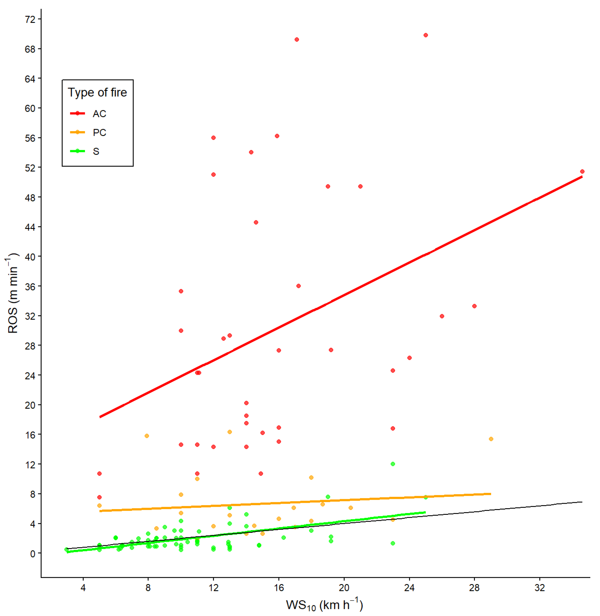
Before fitting surface fire models, the database of combined surface and crown fire observations was explored for overall trends and patterns. Among 127 fires in conifer stands, a clear, though noisy linear relationship is evident between ROS and type of fire, as shown in an ROS-WS10 graph (Figure 2).
Surface fire ROS in the main training dataset ranged from 0.4 to 12.0 m min−1, driven by wind speeds of 2.7–28.0 km h−1 and FFMC values of 80.0–94.1. Combined, these conditions generated an ISI range of 2.3–28.7. In conifer stands, surface and passive crown fire spread observations overlapped for ROS > ~4 m min−1 (Figure 2), and most fires’ sROS values were well below the maximum value (95th percentile sROS of 5.83 m min−1). The fitted linear trends in Figure 2 represent very simple baseline models for conifer ROS observations based on type of fire and wind speed. While the relationships are highly variable for crown fires, the fit is much better for surface fires, showing the lowest variance of the three fire types (Model 1 (M1), n = 67; RMSE = 1.59, adjusted R2 = 0.315). Noting that the M1 intercept was small and nonsignificant ( β 0 = 0.57, P = 0.260) and the fitted slope between 1/5 and 1/4 ( β 1 = 0.244), some simple heuristic models were evaluated as R O S = β 1 W S 10 , with both ROS and WS10 values in their original units of km h−1 and m min−1. As shown in Figure 2, the best performer was β 1 = 0.2 (RMSE = 1.602), characterized henceforth as M20, or the ‘20% WS10’ model.

3.2. Initial Model Evaluation and Selection

The extensive search among the possible predictor variables revealed ISI and ISIsa to be strong predictors of ROS. The best 1–5-variable sROS predictor combinations all contained one of these variables. In particular, ISI2, ISI, and ISIsa2 were the best single predictors, depending on the dataset being evaluated (Table S3). SFC was significant in some models, as was Fuel Type (FT). Model forms using > 2 predictors were generally non-significant (α = 0.05), reflecting the limited sample size and high variability. After completing the search, terms not appearing in any of the best three combinations were dropped from testing. Certain predictor combinations were also rejected for illogical behaviour or suspected multi-collinearity. For instance, models were rejected if they included both ISI and ISIsa terms, or included either spread index along with WS10 or FFMC (mcsa in the case of the ISIsa), since the spread indices already incorporate both wind and estimated litter moisture influences, and these combinations imply overfitting.
Following the testing, four main sROS model categories were identified: models representing all forest types (‘aggregated’, AGG) and models exclusively for hemi-boreal conifer forests (‘boreal conifer’, BOCON); and models using the base FWI predictors (FFMC, ISI) vs. those using the stand-adjusted moisture estimates (mcsa, ISIsa). Response functions were mostly forced through the origin to avoid over- and under-prediction under low danger conditions (e.g., ISI < 2) and in order to produce models that are usable across a broad range of wildfire conditions (i.e., ISI or ISIsa values of 0–25 or higher); linear models with fitted intercepts tended to produce negative ROS predictions near the origin.

3.3. Refined Surface Fire Dataset, FT and SFC

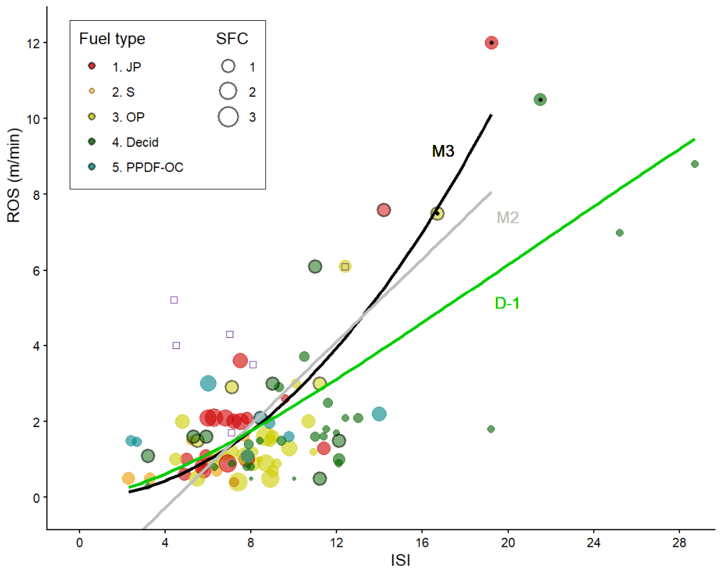
Figure 3 shows sROS observations by ISI, along with some initial exploratory models as well as the D-1 FBP model, with fires classified by FT and SFC. While all fires were classed as surface fires in the original sources, several observations included descriptions of significant torching behaviour, or non-zero levels of measured canopy fuel consumption (CFC).
After further examination of photographs and additional fire documentation [60,61], observations with estimated CFC > 0.2 kg m−2 or obvious evidence of widespread torching were removed in order to exclude fires considered transitional to crown fire, as the ROS of some passive crown fires (but not all) can be much higher than surface fires (Figure 2). Figure 3 also shows a simple linear sROS model fitted to the initial data (BOCON0) based on ISI (M2: RMSE = 1.51; ER2 = 0.464), as well as the better-fitting quadratic model using ISI2 (M3: RMSE = 1.30; ER2 = 0.604).
Fuel type differences in the AGG data were initially evaluated with an ISI2-based linear model similar to M3, and later with the oblique asymptote non-linear form (Equation (4); see Section 3.4 below). All FT contrasts were significant between BOCON, deciduous, and ‘cured condition’ PPDF fuels (Tukey HSD: α = 0.05), with deciduous < BOCON < PPDF in terms of main effects’ influences on ROS. The ‘original curing’ PPDF FT class was not significantly different than the BOCON FT (Figure 3). Within the BOCON dataset, FT was separately tested as follows: there were 19 fires in pure jack pine (JP), 6 in black spruce and mixed pine–spruce (SP), and 26 in stands of other pine species (OP), consisting of red pine (16 fires), and lodgepole pine (10 fires), including the two fires in MPB-affected pine. While FT appeared significant in several models with the conifer dataset, the only significant contrast was between OP and JP, with OP fires predicted to have slightly slower ROS compared with JP fires (Figure 3). This contrast was not deemed meaningful and within-conifer FT was then dropped from further testing.
While SFC did not initially stand out as one of the most influential variables, it was explored further due to its known influence on fire intensity. The sqrt(SFC) predictor was significant in several model forms when combined with ISI, but not ISIsa. Density class initially appeared significant but appeared confounded with the ISIsa and was subsequently dropped.

3.4. Final Fitted Models

Additional models were fitted based on the best variables from the extensive search using the sigmoidal and power function equations described in Section 2.3. Table 1 shows evaluation metrics for a partial list of fitted models, in order of increasing complexity. The full list of tested models and estimates can be found in Appendix B. Table 1 also shows ROS predictions at three levels of ISI or ISIsa (5–15) for comparison. Other variables (FFMC, FT) were assigned values where required for calculation purposes, as noted. The number of observations used in model fitting varied depending on measured and estimated variables available (e.g., missing SFC measurements resulted in slightly smaller datasets for SFC-requiring models) as well as the aforementioned cleaning of transitional crown fire observations. Models M1 and M20 were based on the full set of conifer and unaltered PPDF observations (N = 67; CON; Figure 1), while other models used either the aforementioned ‘AGG’ dataset (N = 80–93) with combined conifer, deciduous and PPDF fires (OC or CC), or the ‘BOCON’ dataset (N = 53–58), with only boreal conifer data. M2, M3 and M4 included all sROS fires (BOCON0; Figure 3), while other BOCON-based models excluded torching fires, as previously noted. The FBP and Van Wagner models (Table 1: C-3s, C-4s, C-6s, D-1) are also shown for comparison purposes. The new models shown predict mean ROS under ISI (or ISIsa) 5, 10, and 15 conditions of 0.7 m min−1, 2.7 m min−1, and 5.1 m min−1, respectively. Model forms using the BOCON data (e.g., M3, M12, M13) had lower variability and thus better overall performance (lower RMSE, higher ER2, lower MAE and MAPE) than similar model forms fitted to the AGG dataset (M6, M10, M11; Appendix B).
The best performing models varied depending on the choice of dataset and available inputs. Non-linear model forms using Equation (1) or Equation (4) were unable to automatically fit the asymptote parameters, so visual inspection was used to estimate asymptotes (m = 0.15, iagg = 10, icon = 13, for AGG and BOCON datasets, respectively). This allowed for the fitting of relatively high-performing models for the aggregated and conifer datasets (M11c, M12–13). The best performance overall was achieved by the models with separate wind and litter moisture inputs (e.g., M16: ER2 = 0.786; see also Appendix B). Certain AGG models were fitted separately depending on the PPDF curing assumption. As noted, original curing PPDF fires were consistent with BOCON fires when using ISI as a predictor (e.g., M7), while ‘cured condition’ ROS appeared more consistent with BOCON fires when using the ISIsa due to the additional mcsa inputs and influence, which reduced estimated fuel moisture conditions. In general, for the AGG data models, the best performance was achieved when SFC (M7) or FT (M18c) were included as predictors compared with only wind and moisture variables.
In addition to the fitted models, Table 1 also compares sROS predictions from the FBP, Van Wagner [16], and 20% WS10 (M20) models. For the C-4s and C-6s, the high MAE and MAPE values, and very low values for ER2, suggest very poor performance compared to the fire observations. The C-3s, D1, and M20 models, in contrast, are at the lower end of the range of model performance but otherwise produce adequate results. When evaluated against the deciduous data alone, the D-1 model produced a reasonably good fit with the data, in the mid-range of the main fitted BOCON and AGG models (Table 1). Note that the D-1 model dataset originally described by [6] differs only from present deciduous database by two additional wildfires, excluded here due to a lack of documentation.

3.5. ISI and ISIsa sROS Models for Conifer and Aggregated Forest Types

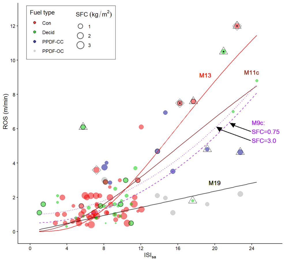
Figure 4 shows the final sROS dataset plotted by overall fuel type (boreal conifer, deciduous, or PPDF) and SFC against ISIsa, along with four fitted conifer models: M9 (AGG data, two SFC levels), M11 (AGG), M13 (BOCON), and M19 (PPDF, OC). PPDF fires with CC ROS were included in model fitting for the AGG data models. Certain high-influence observations are highlighted, based on ‘jackknife’ (leave-one out) resampling. These were flagged when the difference between model parameters was calculated with and without individual estimates, Δ , was Δ > 2 s n , where s is the standard error of the parameter estimate and n is the sample size [62]. This shows how the high ISIsa observations, including most of the wildfires, were particularly influential on the fitted models.

3.6. Model Validation

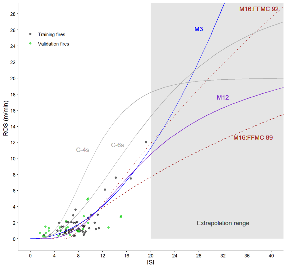
The validation dataset included mean WS10 and ISI values of 12.3 km h−1 and 6.8, respectively (WS10 range: 2.8–23.8 km h−1; ISI range: 1.6–15.0). A wide range of experimental fire conditions was therefore represented (Figure 5). No attempt was made to estimate the mcsa stand structure and condition categories; consequently, only ISI- or WS10- and FFMC-based models were tested.
Models M12, M16, and M20 were evaluated with the additional validation observations (Table 2). All three models performed well, with MAE and RMSE values < 2 m min−1. The best performance based on these measures was from M16, with the lowest MAE, MAPE and Mean Bias Error (MBE), while M20, the simple wind speed heuristic, had the lowest (best) RMSE, indicating the influence of some wider outliers. The accuracy differences between M16 and M12 in training, where M16 had a slightly lower (better) MAPE, by 0.029, and lower (better) MAE by 0.061 m min−1 (Table 1), were not fully replicated during validation, as M16 had the lower MAE while M12 had the lowest MAPE (MAE: M16 lower by 0.028 m min−1; MAPE: M12 lower by 0.018; Table 2). M20 exhibited the highest MBE, showing a consistent overprediction tendency of about 0.9 m min−1, notably higher than the other two tested models, which had very small underprediction biases of <0.15 m min−1, although M16 had the slightly superior value.
Figure 5 shows the BOCON training data plotted by ISI, comparing some of the highest-performing ISI-based models (M3, M12, M16) along with the validation data. The observation space beyond the range of data is shaded, representing extrapolation. All three models produce fairly similar ROS predictions within the range of data but diverge widely when ISI > ~20. Figure 5 also shows the C-6s and C-4s models, which both overpredict ROS for most conifer observations.

4. Discussion

4.1. Operational Surface ROS Models

Since wildfire spread under higher danger conditions in conifer stands tends to be from crown fires [63,64], it is unsurprising that the majority of surface fires in our database occurred during moderate-level fire danger indices and wind speeds. Crown fire occurrence in conifer forests has long been modelled using canopy base height and surface fire intensity [26] or surface fuel consumption [25,65]. This explains the existence of a few conifer surface fires (primarily in high-CBH pine stands) in our database that occurred under dry and windy conditions (ISI > 10). Our database shows that ROS in deciduous stands is broadly similar to surface fire ROS conifer stands, though slightly slower-spreading based on the significant fuel type factor in models M18/M18c (Table 1).
Because of the dearth of experimental data from fires ignited under high-danger conditions, a small number of wildfires exhibiting surface fire behaviour were also included to populate the higher range of ISI/ISIsa values. Being few in number, individual high-danger observations tended to be highly influential in regression models (Figure 4). Despite this warning, there is no way of removing these observations without significantly affecting the models and their range of inference. Primary source descriptions that exist for these wildfires (e.g., [66]) tend to reflect simple estimation methods; we would expect high error with such a dataset [67], and some of the highest ROS observations are likely overestimates of actual spread rate. Overall, both our training and validation datasets mainly represent a range of ROS values that could be described as ‘moderately slow’ (1–3 m min−1) to ‘moderately fast’ (3–10 m min−1) [60].

4.2. Predictors of Surface ROS

The ISI was the strongest single ROS predictor variable, performing well in either its original or stand-adjusted form (ISIsa). ISI is familiar to Canadian operational practitioners and remains established as a key index of fire weather. It was the most strongly correlated variable to area burned during the record-breaking 2023 Canadian wildfire season [68], and is significantly related to the probability of fire containment in black spruce stands [69]. The database values used in our analysis represent indices that best represent burning conditions according to primary sources. For forecasting purposes, we expect hourly ISI to perform slightly better than daily ISI values when the time of interest differs from the typical afternoon peak burning conditions [70,71]. The ISIsa quantifies additional influences based on stand properties and longer-term moisture effects (i.e., the DMC and ‘season’ variables) [45], and offers additional value for predicting ROS across varying stand structure using models such as M9/M9c or M11/M11c. For typical moderately closed boreal conifer stands of spruce and pine, however, the ISIsa did not tend to improve model performance, and the base ISI may be preferred. The use of ISIsa with M13 or M17 (see Appendix B) may nonetheless provide useful contrasts, such as between density categories or at different DMC levels. It is unclear if small differences in evaluation metrics, such as between ER2 values of 0.74 (M12) and 0.70 (M13), are meaningful; evaluation with independent data including mcsa attributes is needed at this stage to improve confidence.
The overall best-performing model in BOCON stands, with the lowest RMSE and AIC, and highest ER2, was M16, the mcFFMC- and WS10-based model that was not constrained by the fixed fuel moisture and wind speed relationship of the ISI. M16 was also the best performer in the validation data, with the lowest MAE and bias, although the other model tested, M12, performed nearly as well using ISI. The main concern with the quadratic and power function models is a possible tendency to overpredict under high wind conditions. As discussed earlier, wind speed influences on ROS have previously been fitted to power functions as WSb, where b > 1 in some studies but b = 1 or b < 1 more often occur under high wind speeds [9,72]. The fitted b values in our power models (Equation (5)) ranged from about 1.3 (M14, M15c) to 1.9 (M16) (see Appendix B), which results in an accelerating increase in ROS at higher WS or ISI values. The ISI- and ISIsa-based models, in contrast, are heavily influenced by the exponential wind speed function within the ISI equation (Equation (2)). The recommended ISI fix for high winds in the FBP System, whereby the ISI equation is altered when WS10 > 40 km h−1 [15,71], will prevent excessive ROS predictions under such conditions, but is not well-tested. Extreme weather fires are, in any case, well beyond the range of our surface fire dataset, as processes such as crown fire spread, ember spotting and fire–interactions would be expected to dominate ROS, particularly in conifer forest types [73].
Figure 5 further illustrates the concern with extrapolation and uncertainty beyond the range of our data (e.g., ISI > 20, or WS10 > 25 to 30 km h−1 in typical wildfire conditions of FFMC 90 to 92 or higher). While validating sROS in this range would require much more surface fire data under dry and windy conditions, it is unlikely that understory surface fires would match the spread rates of active crown fires (e.g., ROS > 20 m min−1; Figure 2; see also [74]). The oblique asymptote (M10, M12, M13) or linear models (M1, M2, M20) may be less prone to overprediction under extrapolation conditions. While extrapolation is never advised with empirical models, it is not uncommon in wildfire settings (e.g., [11]), as fire personnel often must often contend with drier and windier conditions than appear in experimental datasets.
The present surface fire models involve mainly weather- and moisture-related inputs, with additional influence from fuel type and SFC in some model forms. In-stand ground-level wind speed (‘mid-flame’) is used in several empirical models due to its apparent direct influence on flame properties and propagation [6,48]. We might therefore expect overstory vegetation density or structure to significantly affect ROS in our models, due to the vegetation’s influence on ground-level wind speed and overall micrometeorology [37,75,76]. However, our findings do not support strong fuel type differences, aside from contrasts between conifer, deciduous, and PPDF (OC or CC) fuel types. Density class was only significant within the ISIsa, based on the density class influence on fuel moisture [45]; see Section 4.3 below.
SFC was a useful secondary influence on ROS (M7, M9), similar to the BUI effect on ROS in the FBP System [11]. It is significant to have evidence, albeit limited, for the direct relationship between SFC and ROS in models such as M9c (Figure 4). Given that the median BUI in our training data was 45, the limited influence of SFC is not surprising and suggests that refitting with additional sROS observations under drier conditions will be needed to improve the SFC–ROS relationship. SFC must itself be modelled from fuel loading and moisture indices in most fire forecasting situations [25,46]. While practical methods for estimating SFC exist, such as those based on FWI components [11,77], it is questionable whether the small estimated change from this added variable is worth the effort and uncertainty for most operational users.

4.3. sROS and Stand Density

As wildfire hazard reduction treatments become more widespread, where stands with high CBH and low surface fuel loading are engineered to resist crown fire [63,78], there is a need to estimate the effects of stand density on sROS under higher danger conditions. Although stand density class variables were not significant on their own in our tests, the models using ISIsa account for some density differences. This provides some capability to represent, for instance, forest thinning treatments. Physical modelling studies have suggested that reducing stand density can increase surface ROS [79,80], often an unintended consequence of fuel treatments [81]. However, the effects of such differences in the present sROS models (e.g., M13, M9) are relatively small, as the only relationship being simulated is fuel moisture via the mcsa density categories—‘Dense’ (D), ‘Moderate’ (M), or ‘Light’ (L) [45], tentatively interpreted as canopy closure levels of >60%, ~40–60%, and <40%, respectively. Expected changes due to heightened in-stand winds are not represented. More significant density changes (e.g., following harvesting or post-fire overstory mortality) are also unlikely to be adequately represented by the categories in the mcsa, and in models such as M9 or M13. Note that [25] had previously suggested using the conifer canopy closure categories of <45% and ~45–60% for representing mcsa ‘Light’ and ‘Moderate’ density classes; the revised recommendation of <40% and ~40–60% closure, respectively, follows some additional testing.
For example, in a pine stand under dry, moderately windy conditions (FFMC 92, DMC 120, WS10 = 15 km h−1) in summer, decreasing the density class from D to M or L would result in an increase from 3.5 to 3.7 to 4.6 m min−1, respectively, using Model 9c (assuming SFC of 1.5 kg m−2): a maximum density-dependent difference ( Δ ) of 1.1 m min−1. Varying SFC between 0.5 and 3.5 kg m−2 could further stretch Δ to 1.8 m min−1, holding the weather indices constant. This is a relatively small ROS difference for capturing this wide range of SFC and density conditions, such as tree density reductions of 70–80%, which are common in hazard reduction treatments [82,83]. The present models are likely most appropriate for moderately open to closed conifer stands; a lower limit for ‘Light’ crown closure would be likely to be near 15–20%, the density of the more open PPDF and other BOCON stands. In very open forests and parkland or savannah-type stand structure (closure ≪ 20%), much greater in-stand wind speed would be expected [37,84] and might support significantly faster sROS than appears in our data.

4.4. Expected Accuracy

In addition to MAE and MAPE values (Table 1), quantiles and comparisons with external validation data can help reveal the expected error associated with each model during normal use. Table 3 shows an analysis of the mean and 90th quantile absolute error (MAE, Q90AE, respectively) and absolute percentage error (MAPE, Q90APE, respectively) for models M12, M16, and M20 using base FWI indices (ISI, WS10, mcFFMC), and for model M9c using ISIsa and fuel type. The Q90 metrics, in particular, should contain the great majority of variation encountered during model use within the range of data.
Since the frequency of observations drops off for higher fire-danger levels (Figure 4 and Figure 5), error categories are shown for ISI or ISIsa values above and below 11. As the MAE and Q90AE values in Table 3 suggest, sROS errors of 1–2 m min−1 are to be expected from models M12 and M16 at lower fire-danger levels, while larger errors of perhaps 2–4 m min−1 may be expected under ISI 12–25 conditions. Models M20 and M9c exhibit mostly similar accuracy, though with occasional higher error rate for outlying values, notably underprediction for M20 of up to 6 m min−1; this error rate did not reappear in the validation data. In percentage terms, the error rates are reversed, with greater percent error at low danger levels (20–80% for under-; up to 270% for over-prediction) compared with the higher danger conditions (15–60% for under-; up to 150% for over-prediction) expected with these models (Table 3). This degree of error, though not ideal, is likely acceptable for operational use considering the much higher ROS (and variability) associated with crown fire behaviour (e.g., Figure 2).

4.5. Recommended Models for Operational Forecasting

The primary value of such surface ROS models may be to inform dynamic modelling systems (e.g., [20,21,85]), where tools such as calculators and lookup tables enable users to forecast fire behaviour under various fuel structure and weather scenarios. This study began with a question about fuel type differences in sROS. It is possible that larger FT differences exist but were obscured by variations in experimental design between sites, such as plot size, ignition methods, or the frequency of wind monitoring. Laboratory experiments have suggested that a range of conifer litterbed characteristics, including species and bulk density, can affect heat flux, spread rate and overall flammability [42,86,87]. However, laboratory results can be challenging to relate to the field context, as detailed fuelbed measurements are seldom available at operational scales and complex natural forest fuelbeds are highly heterogeneous [88]. We revisit the original question by noting that the evidence supports some fuel type differences requiring distinct models, but no significant differences among the main boreal conifer types.
In our modelling dataset, deciduous and PPDF observations helped increase the breadth and scope of observations and presented some evidence for fuel type-specific models or terms. For these types, however, no new data was provided beyond the range of the original FBP System D-1 and C-7 spread models. While the D-1 model matches the noisy deciduous fire data adequately, interpreting the PPDF data is more complex; the few available observations are inadequate to support or refute the substantial anecdotal evidence for the influence of grass curing on ROS.
Despite these challenges, a small number of models stand out as superior to the others in terms of performance and practical applicability (Table 4). These are the models that are more likely to predict new observations within a reasonable accuracy range, e.g., +/− ~30% [89], and those that provide new decision-support tools for a defined purpose in fire management. Within the data range (ISI < 20; ISIsa < 25), the arguably best-performing conifer model for closed natural stands was the mc and WS10 power model M16; the mcsa-based analogue, M17, performed nearly as well (Appendix B). The best conifer model that allows for more stand structure flexibility (via the ISIsa), and is also likely more tolerant of extrapolation, is M13; for simple boreal conifer stands, the ISI-based M12 had slightly higher evaluation metrics. To allow for comparisons between broad fuel type classes or SFC levels, M18c (FT) or M9c (SFC) may have value (or M7, for a non-stand-adjusted version), although the SFC effect is subtle, as noted, and the cured PPDF fuel type is untested. M11c is also a ‘do anything’ model that is applicable to surface fire spread across many fuel types, such as continuous mixed wood of varying percentages in spring. There may also be value to an ensemble approach using combinations of these models, resulting in something close to the mean values for ISI 5–15 noted in Table 1. A more serious ensemble modelling approach would likely focus on a particular fuel type class (e.g., boreal conifer) and perhaps exclude the most extreme outliers.
In comparison, the previously published FBP and Van Wagner models were mixed in their performance metrics. Negative ER2 values and MAPE of 150–380% indicate that the C-4s and C-6s models performed worse than a null model using only the mean of all observations. These models are therefore not recommended for predicting surface fire behaviour in boreal conifer stands, as their overprediction tendency is evident. As for the C-3s model, it performed adequately in representing the overall BOCON data, although it is virtually identical to the D-1 model (Figure 1) and this study presents several options that are likely more accurate and flexible.
The only new model with a similarly poor evaluation metric to C-4s was Model 19 for PPDF (original conditions), which also had a negative ER2 value. In that case, it is due to its small sample size and low overall ROS distribution. However, there is little doubt that increasing wind speed and decreasing fuel moisture (i.e., higher ISI) will increase ROS in this fuel type, as in the others, and the other metrics (RMSE, MAE, MAPE) indicate that M19 predicts sROS in PPDF stands quite faithfully under conditions mimicking the original data (primarily spring fires during green-grass conditions; Appendix A).

4.6. Limitations, Final Suggestions, and M20: The ‘1.2–20’ Model

Our dataset of 53–93 surface fire observations appears well-suited to building new sROS models using linear and non-linear regression techniques. As the dataset grows, there may be opportunity to use more sophisticated machine learning methods that reveal additional variables or spread functions [90]. However, we believe that the current models appropriately represent the present range of observations.
As noted, the major limitation of these ROS models and the underlying dataset are the paucity of observations under higher danger conditions (WS10 or ISI). For improving empirical models, there is no substitute for acquiring additional high-quality observations. Surface fire observations spreading under high indices would necessarily have a high LCBH and/or low SFC; otherwise, they would be expected to quickly transition to crown fires [25,65]. Additional high-danger sROS observations are unlikely to come from experimental burning, but could be detected from the opportunistic imaging of spreading wildfires [91,92], such as wildfires burning in tall pine or Douglas-fir stands with CBH > 10 m [93].
Under very-low-danger conditions (e.g., FFMC < 75 or ISI < 1), ignition in needle fuel substrates becomes highly unlikely [94,95], so ROS is a minimal concern until drier and windier conditions arrive. Under such marginal conditions, these models may overpredict fire spread, but this is likely a minor concern given the low predicted ROS, except in situations of very long simulations of several days or longer. For the best compromise between performance and flexibility and general use, we believe the M13 model may be the most useful for boreal and sub-boreal conifer stands, and the M11c model is similar but more fuel-agnostic. The other recommended models are suited to more specific comparisons, as discussed. In particular, using any of the AGG-based models for fires in PPDF stands should only be attempted with an understanding of the assumptions and sparse data associated with this fuel type. Model M19, a very simple linear regression for low-grass-curing conditions using unaltered ROS, is likely the most conservative option. However, for PPDF stands in late- (or very early-) season wildfire conditions, one of the ‘cured condition’ models may be advisable to reduce the possibility of underprediction errors. Since these CC observations were generated based on untested assumptions, they may perform poorly until further tested and calibrated, but will be less likely to underpredict than the OC-based models, or even than the C-7 fuel type [11] below the crown fire threshold.
Finally, the 20% WS10 model will be useful in a similar manner to the Cruz and Alexander ‘10% rule’ [74] and ‘20% rule’ [96] models—as an approximate value suitable for mental arithmetic and rapid field use. With a slope of β 1 =   0.20 and zero intercept, this offers a simple and rapid approximation of the WS10–sROS relationship, easily calculated from wind speed forecasts in multiples of 5 km h−1 (15, 20, 25, etc.); it should perform adequately for WS10 < 30 km h−1 or so. Importantly, the unit difference (km h−1 vs. m min−1) is critical for proper usage; an exact analogy with, for instance, the 10% rule [74] would suggest it should be called the ‘1.2% rule’ model, based on similar wind speed units. We therefore suggest the name ‘1.2–20 Model’ (‘one–two twenty’) to encourage understanding and uptake.
The 1.2–20 heuristic also reveals an additional finding of interest: on average, conifer crown fires are shown to be seven times faster than Canadian experimental surface fires under similar wind speeds. This is calculated from the calculated mean conifer crown fire ROS as 8.4% of the WS10 [74] and the slope of the M20 sROS model, with wind and ROS in identical units (8.4/1.2 = 7). The corollary to this is that any treatment that alters potential fire behaviour from crown fire to surface fire, particularly pruning or ladder fuel removal, which significantly increases the crown base height [25,26,65] can theoretically reduce ROS by 6/7, or about 86%, assuming no other difference but type of spreading fire. This is a very simplistic heuristic-based observation based on distinct studies and datasets, but may prove to be a useful point for consideration and communication. Notably, this simple assessment does not discriminate between passive crown fire and the much higher active crown fire ROS, with type of crown fire spread being dependent on WS and canopy fuel characteristics [26,65], as well as additional atmospheric variables and interactions. If nothing else, this ‘6/7ths of ROS’ observation should be a worthy concept for further testing and refining.

5. Conclusions

This study examined whether experimental observations support the large differences in predicted surface fire ROS among fuel types, and if not, what models best describe subcanopy fire spread in hemi-boreal forests.
Analysis of a fire behaviour dataset from nearly 100 experimental fires in a range of conifer and deciduous forests showed that the ROS of most understory surface fires was below 6 m min−1, with limited observations up to 12 m min−1. Within this range, there was little evidence of a plateau in ROS with increasing wind speed. Surface ROS was approximately one seventh of crown fire ROS under comparable conditions, and a simple heuristic using different units suggests that understory ROS (in m min−1) is approximately one fifth of the 10 m open wind speed (in km h−1).
Models fitted separately to boreal conifer and ponderosa pine datasets were more accurate than equivalent models fitted to aggregated datasets, but there was little evidence to support significant fuel type differences within the boreal conifer observations. Models incorporating wind speed and estimated fuel moisture as separate variables performed slightly better than models based solely on the Initial Spread Index (ISI), but ISI-based models also performed well. Among the model forms evaluated on single variables, a modified Chapman–Richards equation provided the best fit and outperformed linear and quadratic alternatives.
The final models include eight or nine recommended formulations that should suit various purposes in North American fire management. Input variables such as 10-m open wind speed and FWI codes (FFMC, ISI) are readily available to most managers of hemi-boreal forest lands, and these models can easily be integrated into automated decision support tools used by wildfire organizations. The new models are suited to a range of general and specialized purposes. These include everyday operational fire behaviour forecasting; contrasting broad fuel types or stand conditions; designing hazard reduction treatments; and performing additional analyses or simulations. While the data are scattered and the models overall somewhat imprecise, it is evident that a much greater range of ROS magnitude and variability are associated with crown fire spread in conifer stands than for surface fires (e.g., Figure 2). Consequently, the much smaller differences of ~2–3 m min−1 associated with the uncertainty of these models are unlikely to be hazardous to trained fire personnel nor to be insurmountable in daily operations. Fire behaviour practitioners can adopt the recommended models into their operational systems without delay to aid in surface fire forecasting.

Supplementary Materials

The following supporting information can be downloaded at: https://www.mdpi.com/article/10.3390/fire9070302/s1, Table S1: Surface fire observations for model-building; Table S2: Surface fire observations for validation; Table S3: Ranking of predictor variables in model-building.

Author Contributions

Conceptualization, D.D.B.P. and S.W.T.; methodology, D.D.B.P. and S.W.T.; analysis, D.D.B.P.; writing—original draft preparation, D.D.B.P., N.J.R.H. and S.W.T.; writing—review and editing, D.D.B.P., S.W.T. and N.J.R.H.; visualization, D.D.B.P. and N.J.R.H. All authors have read and agreed to the published version of the manuscript.

Funding

This research received no external funding.

Data Availability Statement

Data is available upon request from the corresponding author.

Acknowledgments

We are grateful for helpful comments on the draft provided by D.K. Thompson.

Conflicts of Interest

The authors declare no conflicts of interest.

Abbreviations

The following abbreviations are used in this manuscript:
AGGAggregated forest dataset, includes surface fire observations from all described stand types
BOCONBoreal conifer surface fire dataset
BOCON0Initial boreal conifer surface fire dataset (includes fires with significant torching)
CCuring (grass or herbaceous vegetation)
CBHCrown or canopy base height
CCCured condition—estimated late-season PPDF fire behaviour when grass and herbs are most flammable
CFCCrown or canopy fuel consumption
CONConifer dataset; includes boreal and ponderosa pine–Douglas fir surface fire observations
DECIDDeciduous forest stands
DMCDuff Moisture Code, from the Fire Weather Index System
ER2Efron’s pseudo-R squared
FBPFire Behavior Prediction (System)
FFMCFine Fuel Moisture Code
FTFuel Type
FWIFire Weather Index (System)
ISIInitial Spread Index
ISIsaStand-adjusted Initial Spread Index
MAEMean Absolute Error
MAPEMean Absolute Percentage Error
MBEMean Bias Error
mcMoisture content (litter)
mcFFMCMoisture content (litter), estimated from the Fine Fuel Moisture Code
mcsaStand-Adjusted Moisture Content (litter)
OCOriginal Curing—fire behaviour in PPDF stands as observed, with high moisture in grass and herbs
PPDFPonderosa pine–Douglas fir forest stands (see also ‘CC’ and ‘OC’ conditions)
RMSERoot Mean Squared Error
ROSRate of Spread
sROSSurface Rate of Spread
SFCSurface Fuel Consumption
WS or WS10Wind Speed; general or open 10 m wind speed

Appendix A. Fires in Ponderosa Pine–Douglas-Fir Stands in BC

Eight experimental fires were conducted in 1978–80 in open Ponderosa pine–Douglas fir (PPDF) forest stands in the Lower Dewdrop Range near Kamloops, British Columbia. These fires were mostly well-documented in theses by Nyberg (plots 1–6) [55] and Smaill (plot 9) [97]. Plot numbers 1–6, burned in 1978, are described by [55]. Plot 9, burned in 1979, is described by [97]. Plot 8 from the same site was burned in 1980, with rudimentary documentation (FWI indices, ROS) provided by the FBP System experimental fire database. Summary information and photographs were incorporated into the FBP System in the form of the C-7 fuel type, where these experimental data were combined with several wildfire observations to fit and estimate the various fuel type functions and parameters [11,98]. Note that some tools exist for calculating ROS with the unpublished ‘C-7b’ model [56], a version of the C-7 FBP fuel type that allows for adjustments to the grass curing. The C-7b is based on the premise that the C-7 observations, most of which are the PPDF observations in the present study, represent 100% cured-grass conditions. Since this study presents evidence to the contrary (see Appendix A.2), the C-7b can only reduce predicted ROS below the values from the fitted C-7 ROS model, and may therefore be prone to significant underprediction.
For this study, the Lower Dewdrop PPDF observations were reanalyzed from the original document records in order to merge these fires into the main modelling database with common units and analysis methods. Stand structure at the Lower Dewdrop consisted of a low-density Ponderosa pine-dominated overstory and mostly herbaceous understory, with mean canopy closure of approximately 32%. Litter and duff cover were described as light and patchy [55].

Appendix A.1. Surface Fuel Consumption

In the FBP System database (and C-7 fuel type), surface fuel consumption (SFC) was reported for only one observation (Plot 9), with a very high total SFC value of 5.3 kg m−2, dominated by >5 kg m−2 of woody fuel consumption. The original SFC estimate for Plot 9 included consumption of all downed woody fuels, including from large-diameter coarse woody debris (CWD; >7.6 cm). While methodologically consistent with other FBP experimental burns [17,18], the Plot 9 CWD consumption represents the great majority of the total SFC and represents an outlier compared to other FBP System experiments. For instance, the mean CWD proportion of SFC at the Ontario Kenshoe Lake and Sharpsand Creek sites was 9.2%, c.f., [17,18], significantly lower than the 50.2% CWD proportion of consumption at Dewdrop (Mann–Whitney U-test: p < 0.001). This difference is explained by both higher seasonal drought conditions during the Dewdrop burns (mean Drought Code (DC): 394 at Dewdrop vs 111 at Kenshoe Lake and 161 at Sharpsand; see [13] for DC description), and probably the overall frequency of larger-diameter standing trees at Dewdrop, the source of the CWD (>17% of trees in the ‘ >25 cm’ DBH class; c.f., [55]); compared with, e.g., ~1% of trees in the ‘>23 cm’ DBH class at Kenshoe Lake (‘White River’) [99].
Including contributions from CWD in surface fires is somewhat at odds with the current understanding of flame-front dynamics. Consumption studies suggest that most CWD consumption in PPDF stands occurs during post-frontal smouldering rather than during flaming combustion [100,101]. The high SFC at Dewdrop from smouldering CWD, unrelated to the actual flame front, could therefore overpredict fire intensity as well as crown fire tendency [25,26]. To correct this discrepancy, new SFC values at Dewdrop were calculated, excluding the CWD contribution, including only consumption from finer fuels (grass and herbs, litter, duff, and woody debris < 7.6 cm). Calculated SFC was 0.50–1.42 kg m−2 for Plots 1–6, c.f., [55] and the new Plot 9 value was notably lower, at 1.95 kg m−2. Note that SFC estimates represent the differences between pre-burn and post-burn fuel loading, including contributions from woody fuels, grasses and forbs, and litter (the site featured negligible duff quantities). Estimating litter consumption values required an estimate of pre-burn litter depth, which was not reported but was instead taken from [50], a later series of experiments at a very similar site < 5 km away. (Mean litter depth from control sites across all years and canopy positions was 3.3 cm.)

Appendix A.2. Seasonal Climate and Herbaceous Curing

The climate during the 1978 fire season, as well as the timing of the Dewdrop experiments, may have also been somewhat anomalous compared to typical PPDF wildfires; both factors are likely influential in how the Dewdrop data and ensuing models should be treated. Measurable rainfall was received at the Dewdrop weather station nearly weekly from April–August [55], an unusual occurrence in this summer–dry climate. In addition, five of the eight Dewdrop burns were conducted in May or June—growing season months with typically high herbaceous moisture. Consequently, understory vegetation remained relatively green during the experimental fires. Relative proportions of live and dead grass and forb biomass were used to calculate percent curing values (C) for these observations, in the same manner as used in Australian and Canadian grass fire models [15,102]:
C = G B D G B D + G B L 100 ,
where % C is the curing (%), and GBD and GBL represent dead and live grass and forb biomass (kg m−2), respectively. Using mean values from experimental and control plot sampling on each given date [55] gave % C values of 56–66 for Plots 1–6. The curing factor, CF was then calculated using the simple FBP System grass-curing function that combines a gradual exponential rise at low C levels with a linear function at higher curing [15]:
C F = 0.005 e x p 0.061 C 1 , C < 58.8 ,
and
C F = 0.176 + 0.02 C 58.8 ,   C 58.8 ,
For Plot 9, reported values are unfortunately less explicit between live and dead biomass [83] and Equation (A1) could not be used. Based on the late season date and slightly lower overall grass moisture value, % C for that plot was estimated at 80%. For Plot 8, another early season fire (12 June), the mean curing value for Plots 1–6 was used [57].

Appendix A.3. Modelling PPDF Fires

As noted in the main text, we calculated an estimated 95% C ROS for these fires based on two assumptions: (1) detrending of the measured and estimated herbaceous curing values noted above would occur, and (2) these stands would be affected by herbaceous curing half as much as a true grassland, due to the significant influence from other dead fine fuels (mostly litter and fine woody debris). This new modified value was calculated as ROS′ using the following modified curing equation:
R O S = R O S 0 2 1 + c f 95 c f C ,
where ROS0 represents the observed rate of spread with measured curing C, and cf(C) and cf(95) represent the calculated curing factors [15] at measured or estimated C values and 95% C, respectively. ROS’ values for these seven PPDF fires were then used in fitting certain models, as noted in the main text.
These analyses allowed us to incorporate the dry PPDF Dewdrop experimental fires in our surface fire models (AGG data), including sROS models for the measured and 95% cured conditions. Because of the significant assumptions, these models should only be used with caution; actual ROS values in cured-grass PPDF stands may be higher or lower than those estimated using the ‘cured conditions’ models with the PPDF fuel type, for a variety of reasons. While a more generalized PPDF sROS model that incorporates variable grass curing would clearly be useful, the present data are insufficient for anything more refined.

Appendix B. Final Model Estimates

Table A1. Coefficients and statistics for all models discussed in main text. N refers to the number of observations; Coef. indicates coefficients, SE is standard error, and ER2 is Efron’s pseudo-r squared.
Model *FormulaDataset *NCoef.EstimateSEStatisticPER2
1β0 + β1·WS10CON67β0−0.572480.5042−1.1360.26030.325
β10.244310.04365.6<0.0001-
2β0 + β1·ISIBOCON058β0−1.702530.5755−2.9590.00450.464
β10.481080.06916.967<0.0001-
3β1·ISI2BOCON058β10.028260.001915.133<0.00010.604
4β1·ISIsa2BOCON058β10.023520.001714.018<0.00010.553
5β1·WS102BOCON53β10.013080.001211.059<0.00010.450
6β1·ISI2AGG93β10.015900.00115.444<0.00010.461
7β1·ISI2 + β2·sqrt(SFC) AGG80β10.012500.00112.082<0.00010.607
β20.698080.16764.166<0.0001-
8β1·ISIsa2AGG93β10.015690.00114.766<0.00010.426
8cβ1·ISIsa2AGG93β10.017840.00117.930<0.00010.549
9β1·ISIsa2 + β2·sqrt(SFC) AGG80β10.012600.001210.422<0.00010.529
β20.577040.19282.9920.0037-
9cβ1·ISIsa2 + β2·sqrt(SFC) AGG80β10.014730.001113.191<0.00010.649
β20.594300.17813.3380.0013-
10 * m · I S I · i · 1 ( e b · I S I ) c AGG93b0.065870.01175.640<0.00010.548
c2.272050.42665.327<0.0001-
11 * m · I S I s a · i · 1 ( e b · I S I s a ) c AGG93b0.051000.01124.541<0.00010.450
c1.842580.37994.850<0.0001-
11c * m · I S I s a · i · 1 ( e b · I S I s a ) c AGG93b0.066800.01116.042<0.00010.579
c2.202540.39785.537<0.0001-
12 * m · I S I · j · 1 ( e b · I S I ) c BOCON53b0.128320.01627.923<0.00010.742
c5.246221.04355.028<0.0001-
13 * m · I S I s a · j · 1 ( e b · I S I s a ) c BOCON53b0.096610.01436.756<0.00010.704
c3.841720.76805.002<0.0001-
14 a · W S 10 b · e c · m c F F M C AGG93a0.528950.27881.8970.0610.590
b1.319710.131110.07<0.0001-
c−0.19720.0340−5.802<0.0001-
15 a · W S 10 b · e c · m c s a AGG93a0.144780.08111.7860.07750.500
b1.457870.16388.903<0.0001-
c−0.103190.0297−3.4750.0008-
15c a · W S 10 b · e c · m c s a AGG93a0.512920.24172.1220.03660.582
b1.289740.13609.484<0.0001-
c−0.179770.0299−6.008<0.0001-
16 a · W S 10 b · e c · m c F F M C BOCON53a0.398130.21221.8760.06650.786
b1.913990.140113.661<0.0001-
c−0.315510.0438−7.207<0.0001-
17 a · W S 10 b · e c · m c s a BOCON53a0.296290.16611.7830.08060.755
b1.698390.152811.116<0.0001-
c−0.232600.0348−6.681<0.0001-
18 * m · I S I · i · 1 e b · I S I c + e · D E C I D AGG93b0.070940.0125.897<0.00010.572
c2.251990.40325.585<0.0001-
e−0.744450.327−2.2760.0252-
18c  * m · I S I · i · 1 e b · I S I c +
d · P P D F + e · D E C I D
AGG93b0.072070.01225.916<0.00010.618
c2.281890.41515.498<0.0001-
d2.695680.52525.133<0.0001-
e−0.760900.3346−2.2740.0253-
19 *β1·ISIsaPPDF8β10.117710.02255.2420.0012−1.54
20  *20% WS10-67-0.2---0.37
* Notes: Dataset refers to the observations used to fit models as well as for the intended use. CON—all conifer; BOCON0—initial uncleaned boreal conifer; BOCON—cleaned boreal conifer; AGG—aggregated fuel types, including BOCON, deciduous, and PPDF. Underlined models are recommended for operational use, as noted in main text (Table 4). Models with a ‘c’ use CC PPDF data; all others use OC PPDF data. For models M10-M13 and M18-M18c, m = 0.15, i = 10, and j = 13. For models 18 and 18c, DECID and PPDF are dummy variables set to 0 or 1 according to fuel type. M18: conifer or OC PPDF (default): DECID = 0; Deciduous stand: DECID = 1. M18c: conifer stand (default): PPDF = 0, DECID = 0; CC PPDF stand: PPDF = 1, DECID = 0; DECID stand: PPDF = 0, DECID = 1. M19 is for OC PPDF stands only. M20 contains no fitted parameters and therefore has no fit statistics. Shading indicates coefficients associated with individual models.

References

  1. Van Wagner, C.E. Describing Forest Fires—Old Ways and New. For. Chron. 1965, 41, 301–305. [Google Scholar] [CrossRef] [Scilit]
  2. Sullivan, A.L.; Gould, J.S. Wildland Fire Rate of Spread. In Encyclopedia of Wildfires and Wildland-Urban Interface (WUI) Fires; Springer: Berlin/Heidelberg, Germany, 2020; pp. 1095–1098. [Google Scholar]
  3. Alexander, M.E.; Cruz, M.G. Crown Fire Dynamics in Conifer Forests. In Synthesis of Knowledge of Extreme Fire Behavior: Volume 2 for Fire Behavior Specialists, Researchers, and Meteorologists; Werth, P.A., Ed.; General Technical Report PNW-GTR-891; USDA Forest Service Pacific Northwest Research Station: Portland, OR, USA, 2016; pp. 163–258. [Google Scholar]
  4. Wang, X.; Parisien, M.-A.; Flannigan, M.D.; Parks, S.A.; Anderson, K.R.; Little, J.M.; Taylor, S.W. The Potential and Realized Spread of Wildfires Across Canada. Glob. Change Biol. 2014, 20, 2518–2530. [Google Scholar] [CrossRef] [Scilit]
  5. Wheatley, M.; Wotton, B.M.; Woolford, D.G.; Martell, D.L.; Johnston, J.M. Modelling Initial Attack Success on Forest Fires Suppressed by Air Attack in the Province of Ontario, Canada. Int. J. Wildland Fire 2022, 31, 774–785. [Google Scholar] [CrossRef] [Scilit]
  6. Rothermel, R.C. A Mathematical Model for Predicting Fire Spread in Wildland Fuels; Research Paper RP-INT-115; USDA Forest Service Intermountain Forest and Range Experiment Station: Ogden, UT, USA, 1972.
  7. Andrews, P.L. The Rothermel Surface Fire Spread Model and Associated Developments: A Comprehensive Explanation; General Technical Report RMRS-GTR-371; USDA Forest Service, Rocky Mountain Research Station: Fort Collins, CO, USA, 2018; 121p.
  8. Sullivan, A.L. Wildland Surface Fire Spread Modelling, 1990–2007. 1: Physical and Quasi-Physical Models. Int. J. Wildland Fire 2009, 18, 349–368. [Google Scholar] [CrossRef] [Scilit]
  9. Fernandes, P.M.; Botelho, H.S.; Rego, F.C.; Loureiro, C. Empirical Modelling of Surface Fire Behaviour in Maritime Pine Stands. Int. J. Wildland Fire 2009, 18, 698. [Google Scholar] [CrossRef] [Scilit]
  10. Tanskanen, H.; Granström, A.; Larjavaara, M.; Puttonen, P.; Tanskanen, H.; Granström, A.; Larjavaara, M.; Puttonen, P. Experimental Fire Behaviour in Managed Pinus Sylvestris and Picea Abies Stands of Finland. Int. J. Wildland Fire 2007, 16, 414–425. [Google Scholar] [CrossRef] [Scilit]
  11. Forestry Canada Fire Danger Group. Development and Structure of the Canadian Forest Fire Behavior Prediction System; Information Report ST-X-3; Forestry Canada, Science and Sustainable Development Directorate: Ottawa, ON, Canada, 1992.
  12. Tymstra, C.; Bryce, R.W.; Wotton, B.M.; Taylor, S.W.; Armitage, O.B. Development and Structure of Prometheus: The Canadian Wildfire Growth Simulation Model; Information Report NOR-X-417; Natural Resources Canada Canadian Forest Service: Edmonton, AB, Canada, 2010.
  13. Van Wagner, C.E. Development and Structure of the Canadian Forest Fire Weather Index System; Forestry Technical Report 35; Canadian Forest Service, Petawawa National Forestry Institute: Chalk River, ON, Canada, 1987.
  14. Van Wagner, C.E. Prediction of Crown Fire in Conifer Stands. In Proceedings of the 10th Conference on Fire and Forest Meteorology, Ottawa, ON, Canada, 17–21 April 1989; McIver, D.C., Ed.; Canadian Forestry Service, Petawawa National Forestry Institute: Chalk River, ON, Canada, 1989; pp. 207–212. [Google Scholar]
  15. Wotton, B.M.; Alexander, M.E.; Taylor, S.W. Updates and Revisions to the 1992 Canadian Forest Fire Behavior Prediction System; Information Report GLC-X-10; Natural Resources Canada, Canadian Forest Service, Great Lakes Forestry Centre: Sault Ste. Marie, ON, Canada, 2009.
  16. Van Wagner, C.E. Prediction of Crown Fire Behavior in Two Stands of Jack Pine. Can. J. For. Res. 1993, 23, 442–449. [Google Scholar] [CrossRef] [Scilit]
  17. Stocks, B.J. Fire Behavior in Immature Jack Pine. Can. J. For. Res. 1987, 17, 80–86. [Google Scholar] [CrossRef] [Scilit]
  18. Stocks, B.J. Fire Behavior in Mature Jack Pine. Can. J. For. Res. 1989, 19, 783–790. [Google Scholar] [CrossRef] [Scilit]
  19. Alexander, M.E.; Cruz, M.G.; Lopes, A.M.G.; Viegas, D.X. CFIS: A Software Tool for Simulating Crown Fire Initiation and Spread. In Proceedings of the Vth International Conference on Forest Fire Research, Figueira da Foz, Portugal, 27–30 November 2006; Viegas, D.X., Ed.; Elsevier, B.V.: Amsterdam, The Netherlands, 2006. [Google Scholar]
  20. Perrakis, D.D.B.; Cruz, M.G.; Alexander, M.E.; Taylor, S.W.; Beverly, J.L. Linking Dynamic Empirical Fire Spread Models: Introducing Canadian Conifer Pyrometrics. In Proceedings from the 6th Fuels and Fire Behaviour Conference, Marseille, France, 29 April–3 May 2019; International Association of Wildland Fire: Missoula, MT, USA, 2020. [Google Scholar]
  21. CFS Fire Danger Group. Overview of the Next Generation of the Canadian Forest Fire Danger Rating System; Information Report GLC-X-26; Natural Resources Canada-Canadian Forest Service, Great Lakes Forestry Centre: Sault Ste. Marie, ON, Canada, 2021.
  22. Cruz, M.G.; Butler, B.W.; Alexander, M.E.; Forthofer, J.M.; Wakimoto, R.H. Predicting the Ignition of Crown Fuels Above a Spreading Surface Fire. Part I: Model Idealization. Int. J. Wildland Fire 2006, 15, 47–60. [Google Scholar] [CrossRef] [Scilit]
  23. Alexander, M.E.; Quintilio, D. Perspectives on Experimental Fires in Canadian Forestry Research. Math. Comput. Model. 1990, 13, 17–26. [Google Scholar] [CrossRef] [Scilit]
  24. Cruz, M.G. Modeling the Initiation and Spread of Crown Fires. Master’s Thesis, University of Montana, Missoula, MT, USA, 1999. [Google Scholar]
  25. Perrakis, D.D.B.; Cruz, M.G.; Alexander, M.E.; Hanes, C.C.; Thompson, D.K.; Taylor, S.W.; Stocks, B.J. Improved Logistic Models of Crown Fire Probability in Canadian Conifer Forests. Int. J. Wildland Fire 2023, 32, 1455–1473. [Google Scholar] [CrossRef] [Scilit]
  26. Van Wagner, C.E. Conditions for the Start and Spread of Crown Fires. Can. J. For. Res. 1977, 7, 23–34. [Google Scholar] [CrossRef] [Scilit]
  27. Perrakis, D.D.B.; Lanoville, R.A.; Taylor, S.W.; Hicks, D. Modeling Wildfire Spread Rates in Mountain Pine Beetle-Affected Forest Stands, British Columbia, Canada. Fire Ecol. 2014, 10, 10–35. [Google Scholar] [CrossRef] [Scilit]
  28. Alexander, M.; Sando, R. Fire Behavior and Effects in Aspen-Northern Hardwood Stands. In Proceedings of the 10th Conference on Fire and Forest Meteorology, Ottawa, ON, Canada, 17–21 April 1989; Canadian Forest Service and Environment Canada: Ottawa, ON, Canada, 1989; pp. 17–21. [Google Scholar]
  29. Quintilio, D.; Alexander, M.E.; Ponto, R.L. Spring Fires in a Semimature Trembling Aspen Stand in Central Alberta; Information Report NOR-X-323; Natural Resources Canada Canadian Forest Service, Northern Forestry Centre: Edmonton, AB, Canada, 1991.
  30. Van Wagner, C. Rough Prediction of Fire Spread Rates by Fuel Type; Information Report PS-X-42; Environment Canada Forestry Service, Petawawa Forest Experiment Station: Chalk River, ON, Canada, 1973.
  31. Lawson, B.D.; Armitage, O.B. Weather Guide for the Canadian Forest Fire Danger Rating System; Natural Resources Canada, Northern Forestry Centre: Edmonton, AB, Canada, 2008.
  32. Murphy, P.J.; Woodard, P.M.; Quintilio, D.; Titus, S.J. Exploratory Analysis of the Variables Affecting Initial Attack Hot-Spotting Containment Rate. Can. J. For. Res. 1991, 21, 540–544. [Google Scholar] [CrossRef] [Scilit]
  33. Wotton, B.; McAlpine, R.; Hobbs, M. The Effect of Fire Front Width on Surface Fire Behaviour. Int. J. Wildland Fire 1999, 9, 247–253. [Google Scholar]
  34. Dyrness, C.; Norum, R.A. The Effects of Experimental Fires on Black Spruce Forest Floors in Interior Alaska. Can. J. For. Res. 1983, 13, 879–893. [Google Scholar] [CrossRef] [Scilit]
  35. Van Wagner, C.E. Fire Behaviour Mechanisms in a Red Pine Plantation: Field and Laboratory Evidence; Departmental Pub. No. 1229; Ministry of Forestry and Rural Development, Forestry Branch: Ottawa, ON, Canada, 1968.
  36. Catchpole, W.; Catchpole, E.; Butler, B.; Rothermel, R.; Morris, G.; Latham, D. Rate of Spread of Free-Burning Fires in Woody Fuels in a Wind Tunnel. Combust. Sci. Technol. 1998, 131, 1–37. [Google Scholar] [CrossRef] [Scilit]
  37. Moon, K.; Duff, T.; Tolhurst, K. Sub-Canopy Forest Winds: Understanding Wind Profiles for Fire Behaviour Simulation. Fire Saf. J. 2019, 105, 320–329. [Google Scholar] [CrossRef] [Scilit]
  38. Schlegel, F.; Stiller, J.; Bienert, A.; Maas, H.-G.; Queck, R.; Bernhofer, C. Large-Eddy Simulation Study of the Effects on Flow of a Heterogeneous Forest at Sub-Tree Resolution. Bound.-Layer Meteorol. 2015, 154, 27–56. [Google Scholar] [CrossRef] [Scilit]
  39. Chen, J.; Saunders, S.C.; Crow, T.R.; Naiman, R.J.; Brosofske, K.D.; Mroz, G.D.; Brookshire, B.L.; Franklin, J.F. Microclimate in Forest Ecosystem and Landscape Ecology: Variations in Local Climate Can Be Used to Monitor and Compare the Effects of Different Management Regimes. BioScience 1999, 49, 288–297. [Google Scholar] [CrossRef] [Scilit]
  40. Ma, S.; Concilio, A.; Oakley, B.; North, M.; Chen, J. Spatial Variability in Microclimate in a Mixed-Conifer Forest Before and After Thinning and Burning Treatments. For. Ecol. Manag. 2010, 259, 904–915. [Google Scholar] [CrossRef] [Scilit]
  41. Curry, J.R.; Fons, W.L. Forest-Fire Behavior Studies. Mech. Eng. 1940, 62, 219–225. [Google Scholar]
  42. Campbell-Lochrie, Z.; Walker-Ravena, C.; Gallagher, M.; Skowronski, N.; Mueller, E.V.; Hadden, R.M. Investigation of the Role of Bulk Properties and in-Bed Structure in the Flow Regime of Buoyancy-Dominated Flame Spread in Porous Fuel Beds. Fire Saf. J. 2021, 120, 103035. [Google Scholar] [CrossRef] [Scilit]
  43. Wotton, B.M. Interpreting and Using Outputs from the Canadian Forest Fire Danger Rating System in Research Applications. Environ. Ecol. Stat. 2009, 16, 107–131. [Google Scholar]
  44. Whitehead, R.J.; Russo, G.; Hawkes, B.; Taylor, S.; Brown, B.; Armitage, O.; Barclay, H.; Benton, R. Effect of Commercial Thinning on Within-Stand Microclimate and Fine Fuel Moisture Conditions in a Mature Lodgepole Pine Stand in Southeastern British Columbia; Canadian Wood Fibre Centre Information Report FI-X-004; Natural Resources Canada, Canadian Forest Service: Victoria, BC, Canada, 2008.
  45. Wotton, B.M.; Beverly, J.L. Stand-Specific Litter Moisture Content Calibrations for the Canadian Fine Fuel Moisture Code. Int. J. Wildland Fire 2007, 16, 463–472. [Google Scholar] [CrossRef] [Scilit]
  46. Liu, M.; Greene, G.; Perrakis, D.D.B.; Roeser, D. Modelling Fire Behaviour in the Lodgepole Pine Forests of Interior British Columbia: An Evaluation of Models against Field Evidence. Ecol. Inform. 2026, 95, 103789. [Google Scholar] [CrossRef] [Scilit]
  47. Lumley, T.; Miller, A. Leaps: Regression Subset Selection v3.2, 2024 [Software Package]. Available online: https://cran.r-project.org/web/packages/leaps/index.html (accessed on 31 March 2026).
  48. Anderson, W.R.; Cruz, M.G.; Fernandes, P.M.; McCaw, L.; Vega, J.A.; Bradstock, R.A.; Fogarty, L.; Gould, J.; McCarthy, G.; Marsden-Smedley, J.B. A Generic, Empirical-Based Model for Predicting Rate of Fire Spread in Shrublands. Int. J. Wildland Fire 2015, 24, 443–460. [Google Scholar] [CrossRef] [Scilit]
  49. Mangiafico, S.S. An R Companion for the Handbook of Biological Statistics, Version 1.09, 2015. Available online: https://rcompanion.org/rcompanion (accessed on 31 March 2026).
  50. Ducherer, K.; Bai, Y.; Thompson, D.; Broersma, K. Dynamic Responses of a British Columbian Forest-Grassland Interface to Prescribed Burning. West. N. Am. Nat. 2009, 69, 75–87. [Google Scholar] [CrossRef] [Scilit]
  51. Ducherer, K.; Bai, Y.; Thompson, D.; Broersma, K. Thinning of a Ponderosa Pine/Douglas-Fir Forest in South-Central BC: Impacts on Understorey Vegetation. J. Ecosyst. Manag. 2013, 14, 1–15. [Google Scholar] [CrossRef] [Scilit]
  52. Cruz, M.G.; Gould, J.S.; Kidnie, S.; Bessell, R.; Nichols, D.; Slijepcevic, A. Effects of Curing on Grassfires: II. Effect of Grass Senescence on the Rate of Fire Spread. Int. J. Wildland Fire 2015, 24, 838. [Google Scholar] [CrossRef] [Scilit]
  53. Alexander, M.E. Surface Fire Spread Potential in Trembling Aspen during Summer in the Boreal Forest Region of Canada. For. Chron. 2010, 86, 200–212. [Google Scholar] [CrossRef] [Scilit]
  54. Cheney, N.; Gould, J. Fire Growth in Grassland Fuels. Int. J. Wildland Fire 1995, 5, 237–247. [Google Scholar] [CrossRef] [Scilit]
  55. Nyberg, J.B. Seasonal Effects of Fire on Ponderosa Pine/Bunchgrass Range: Year 1. Master’s Thesis, University of British Columbia, Department of Forestry, Vancouver, BC, Canada, 1979. [Google Scholar]
  56. Beck, J. C-7b Model [Spreadsheet Tool], 2003. In ‘Legacy FBP System-Related Tools’ [Website]. Available online: http://fireresearch.ca/legacy-fbp-system-related-tools/ (accessed on 31 March 2026).
  57. Hicks, D.; Martin, B.; Bowman, B.; Irvine, S.; Levitt, S.; Colwell, R.; Casperson, G.; Spronken, C.; Meyer, E.; Morrow, M.; et al. Various presentations and discussions. In BC Wildfire Service, Fire Behaviour Specialists Working Group, Monthly Meetings; BC Wildfire Service: Victoria, BC, Canada, 2012–2021. [Google Scholar]
  58. Meyn, A.; Taylor, S.W.; Flannigan, M.D.; Thonicke, K.; Cramer, W. Relationship between Fire, Climate Oscillations, and Drought in British Columbia, Canada, 1920–2000. Glob. Change Biol. 2010, 16, 977–989. [Google Scholar] [CrossRef] [Scilit]
  59. Daniels, L.D.; Dickson-Hoyle, S.; Baron, J.N.; Copes-Gerbitz, K.; Flannigan, M.D.; Castellanos-Acuna, D.; Hoffman, K.M.; Bourbonnais, M.; Wilkinson, S.L.; Roeser, D.; et al. The 2023 Wildfires in British Columbia, Canada: Impacts, Drivers, and Transformations to Coexist with Wildfire. Can. J. For. Res. 2025, 55, 1–18. [Google Scholar] [CrossRef] [Scilit]
  60. Alexander, M.; Lanoville, R. Predicting Fire Behavior in the Black Spruce-Lichen Woodland Fuel Type of Western and Northern Canada. [Poster with Text.]; Forestry Canada, Northern Forestry Centre and Government of Northwest Territories, Department of Renewable Resources, Territorial Forest Fire Centre: Edmonton, AB, Canada; Fort Smith, NT, Canada, 1989.
  61. Stocks, B.J.; Hartley, G.R. Fire Behaviour in Three Jack Pine Fuel Complexes [Poster with Text]; Natural Resources Canada—Canadian Forest Service, Great Lakes Forestry Centre: Sault Ste. Marie, ON, Canada, 1995.
  62. Baty, F.; Ritz, C.; Charles, S.; Brutsche, M.; Flandrois, J.-P.; Delignette-Muller, M.-L. A Toolbox for Nonlinear Regression in R: The Package Nlstools. J. Stat. Softw. 2015, 66, 1–21. [Google Scholar] [CrossRef] [Scilit]
  63. Beverly, J.L.; Leverkus, S.E.; Cameron, H.; Schroeder, D. Stand-Level Fuel Reduction Treatments and Fire Behaviour in Canadian Boreal Conifer Forests. Fire 2020, 3, 35. [Google Scholar] [CrossRef] [Scilit]
  64. Cruz, M.G.; Alexander, M.E.; Fernandes, P. Evidence for Lack of a Fuel Effect on Forest and Shrubland Fire Rates of Spread Under Elevated Fire Danger Conditions: Implications for Modelling and Management. Int. J. Wildland Fire 2022, 31, 471–479. [Google Scholar] [CrossRef] [Scilit]
  65. Cruz, M.G.; Alexander, M.E.; Wakimoto, R.H. Modeling the Likelihood of Crown Fire Occurrence in Conifer Forest Stands. For. Sci. 2004, 50, 640–658. [Google Scholar] [CrossRef] [Scilit]
  66. Van Wagner, C. Story of an Intense Crown Fire at Petawawa. Pulp Pap. Mag. Can. 1965, 66, WR 358. [Google Scholar]
  67. Filkov, A.I.; Duff, T.J.; Penman, T.D. Improving Fire Behaviour Data Obtained from Wildfires. Forests 2018, 9, 81. [Google Scholar] [CrossRef] [Scilit]
  68. Jain, P.; Barber, Q.E.; Taylor, S.W.; Whitman, E.; Castellanos Acuna, D.; Boulanger, Y.; Chavardès, R.D.; Chen, J.; Englefield, P.; Flannigan, M.; et al. Drivers and Impacts of the Record-Breaking 2023 Wildfire Season in Canada. Nat. Commun. 2024, 15, 6764. [Google Scholar] [CrossRef] [Scilit] [PubMed]
  69. Beverly, J.L. Time Since Prior Wildfire Affects Subsequent Fire Containment in Black Spruce. Int. J. Wildland Fire 2017, 26, 919. [Google Scholar] [CrossRef] [Scilit]
  70. Beck, J.; Alexander, M.; Harvey, S.; Beaver, A. Forecasting Diurnal Variations in Fire Intensity to Enhance Wildland Firefighter Safety. Int. J. Wildland Fire 2002, 11, 173–182. [Google Scholar] [CrossRef] [Scilit]
  71. CFS Fire Danger Group. The 2025 Update to the FWI System: Structure, Changes, Interpretation; Information Report GLC-X-42; Natural Resources Canada—Canadian Forest Service, Great Lakes Forestry Centre: Sault Ste. Marie, ON, Canada, 2025.
  72. Cruz, M.G.; Alexander, M.E.; Wakimoto, R.H. Development and Testing of Models for Predicting Crown Fire Rate of Spread in Conifer Forest Stands. Can. J. For. Res. 2005, 35, 1626–1639. [Google Scholar] [CrossRef] [Scilit]
  73. Werth, P.A.; Potter, B.E.; Alexander, M.E.; Clements, C.B.; Cruz, M.G.; Finney, M.A.; Forthofer, J.M.; Goodrick, S.L.; Hoffman, C.; Jolly, W.M. Synthesis of Knowledge of Extreme Fire Behavior: Volume 2 for Fire Behavior Specialists, Researchers, and Meteorologists; General Technical Report PNW-GTR-891; USDA Forest Service: Portland, OR, USA, 2016.
  74. Cruz, M.G.; Alexander, M.E. The 10% Wind Speed Rule of Thumb for Estimating a Wildfire’s Forward Rate of Spread in Forests and Shrublands. Ann. For. Sci. 2019, 76, 44. [Google Scholar] [CrossRef] [Scilit]
  75. Amiro, B.D. Comparison of Turbulence Statistics Within Three Boreal Forest Canopies. Bound.-Layer Meteorol. 1990, 51, 99–121. [Google Scholar] [CrossRef] [Scilit]
  76. Dupont, S.; Brunet, Y. Edge Flow and Canopy Structure: A Large-Eddy Simulation Study. Bound.-Layer Meteorol. 2008, 126, 51–71. [Google Scholar]
  77. De Groot, W.; Pritchard, J.; Lynham, T. Forest Floor Fuel Consumption and Carbon Emissions in Canadian Boreal Forest Fires. Can. J. For. Res. 2009, 39, 367–382. [Google Scholar] [CrossRef] [Scilit]
  78. Rutherford, K.H.; Eskelson, B.N.I.; Daniels, L.D.; LeMay, V.; Greene, G.A.; Gray, R.W. Short-Term Impacts of Operational Fuel Treatments on Modelled Fire Behaviour and Effects in Seasonally Dry Forests of British Columbia, Canada. Int. J. Wildland Fire 2025, 34, WF24096. [Google Scholar] [CrossRef] [Scilit]
  79. Parsons, R.A.; Pimont, F.; Wells, L.; Cohn, G.; Jolly, W.M.; de Coligny, F.; Rigolot, E.; Dupuy, J.-L.; Mell, W.; Linn, R.R. Modeling Thinning Effects on Fire Behavior with STANDFIRE. Ann. For. Sci. 2018, 75, 7. [Google Scholar] [CrossRef] [Scilit]
  80. Marshall, G.; Thompson, D.K.; Anderson, K.; Simpson, B.; Linn, R.; Schroeder, D. The Impact of Fuel Treatments on Wildfire Behavior in North American Boreal Fuels: A Simulation Study Using FIRETEC. Fire 2020, 3, 18. [Google Scholar] [CrossRef] [Scilit]
  81. Keyes, C.R.; Varner, J.M. Pitfalls in the Silvicultural Treatment of Canopy Fuels. Fire Manag. Today 2006, 66, 46–50. [Google Scholar]
  82. Prichard, S.J.; Peterson, D.L.; Jacobson, K. Fuel Treatments Reduce the Severity of Wildfire Effects in Dry Mixed Conifer Forest, Washington, USA. Can. J. For. Res. 2010, 40, 1615–1626. [Google Scholar] [CrossRef] [Scilit]
  83. Hirsch, K.G.; Pengelly, I. Fuel Reduction in Lodgepole Pine Stands in Banff National Park. In Proceedings of the Joint Fire Science Conference and Workshop, Boise, ID, USA, 15–17 June 1999; University of Idaho and International Association of Wildland Fire: Boise, ID, USA, 1999; pp. 251–256. [Google Scholar]
  84. Albini, F.; Baughman, R. Estimating Wind Speeds for Predicting Wildland Fire Behavior; Research Paper INT-221; USDA Forest Service Intermountain Research Station: Ogden, UT, USA, 1979.
  85. Hebda, N.J.R.; Perrakis, D.D.B. FuelDash-Conifer Pyrometrics (Online Dashboard), 2024. Available online: https://pfcfire.shinyapps.io/FuelDashR/ (accessed on 31 March 2026).
  86. Cornwell, W.K.; Elvira, A.; Kempen, L.; Logtestijn, R.S.; Aptroot, A.; Cornelissen, J.H.C. Flammability Across the Gymnosperm Phylogeny: The Importance of Litter Particle Size. New Phytol. 2015, 206, 672–681. [Google Scholar] [CrossRef] [Scilit] [PubMed]
  87. Wilson, R.A. Reexamination of Rothermel’s Fire Spread Equations in No-Wind and No-Slope Conditions; Research Paper INT-RP-434; USDA Forest Service Intermountain Research Station: Ogden, UT, USA, 1990.
  88. Mulvaney, J.J.; Sullivan, A.L.; Cary, G.J.; Bishop, G.R. Repeatability of Free-Burning Fire Experiments Using Heterogeneous Forest Fuel Beds in a Combustion Wind Tunnel. Int. J. Wildland Fire 2016, 25, 445–455. [Google Scholar] [CrossRef] [Scilit]
  89. Cruz, M.G.; Alexander, M.E. Uncertainty Associated with Predictions of Surface and Crown Fire Rates of Spread. Environ. Model. Softw. 2013, 47, 16–28. [Google Scholar] [CrossRef] [Scilit]
  90. Jain, P.; Coogan, S.C.; Subramanian, S.G.; Crowley, M.; Taylor, S.; Flannigan, M.D. A review of machine learning applications in wildfire science and management. Environ. Rev. 2020, 28, 478–505. [Google Scholar] [CrossRef] [Scilit]
  91. Hart, H.; Perrakis, D.D.B.; Taylor, S.W.; Bone, C.; Bozzini, C. Georeferencing Oblique Aerial Wildfire Photographs: An Untapped Source of Fire Behaviour Data. Fire 2021, 4, 81. [Google Scholar] [CrossRef] [Scilit]
  92. Valero, M.M.; Rios, O.; Pastor, E.; Planas, E. Automated Location of Active Fire Perimeters in Aerial Infrared Imaging Using Unsupervised Edge Detectors. Int. J. Wildland Fire 2018, 27, 241–256. [Google Scholar] [CrossRef] [Scilit]
  93. Perrakis, D.D.B.; Brown, K.J.; Morrison, K.; Horrelt, D.R.; Taylor, S.W. Assessing Wildfire Potential in a Coastal Forest Watershed, British Columbia, Canada. For. Ecol. Manag. 2025, 590, 122796. [Google Scholar] [CrossRef] [Scilit]
  94. Beverly, J.L.; Wotton, B.M. Modelling the Probability of Sustained Flaming: Predictive Value of Fire Weather Index Components Compared with Observations of Site Weather and Fuel Moisture Conditions. Int. J. Wildland Fire 2007, 16, 161–173. [Google Scholar] [CrossRef] [Scilit]
  95. Nadeem, K.; Taylor, S.; Woolford, D.G.; Dean, C. Mesoscale Spatiotemporal Predictive Models of Daily Human-and Lightning-Caused Wildland Fire Occurrence in British Columbia. Int. J. Wildland Fire 2020, 29, 11–27. [Google Scholar]
  96. Cruz, M.G.; Alexander, M.E.; Kilinc, M. Wildfire Rates of Spread in Grasslands Under Critical Burning Conditions. Fire 2022, 5, 55. [Google Scholar] [CrossRef] [Scilit]
  97. Smaill, G. Seasonal Effects of Fire on Ponderosa Pine/Bunchgrass and Douglas-fir/Pinegrass Ranges; Washington State University: Pullman, WA, USA, 1980. [Google Scholar]
  98. De Groot, W. Examples of Fuel Types in the Canadian Forest Fire Behavior Prediction (FBP) System [Poster with Text.]; Forestry Canada, Northwest Region, Northern Forestry Centre: Edmonton, AB, Canada, 1993.
  99. Walker, J.D.; Stocks, B.J. The Fuel Complex of Mature and Immature Jack Pine Stands in Ontario; Report O-X-229; Great Lakes Forest Research Centre, Canadian Forestry Service, Department of the Environment: Sault Ste. Marie, ON, Canada, 1975.
  100. Monsanto, P.G.; Agee, J.K. Long-Term Post-Wildfire Dynamics of Coarse Woody Debris After Salvage Logging and Implications for Soil Heating in Dry Forests of the Eastern Cascades, Washington. For. Ecol. Manag. 2008, 255, 3952–3961. [Google Scholar] [CrossRef] [Scilit]
  101. Ottmar, R.D. Wildland Fire Emissions, Carbon, and Climate: Modeling Fuel Consumption. For. Ecol. Manag. 2014, 317, 41–50. [Google Scholar] [CrossRef] [Scilit]
  102. Cheney, N.; Gould, J.; Catchpole, W.R. Prediction of Fire Spread in Grasslands. Int. J. Wildland Fire 1998, 8, 1–13. [Google Scholar] [CrossRef] [Scilit]
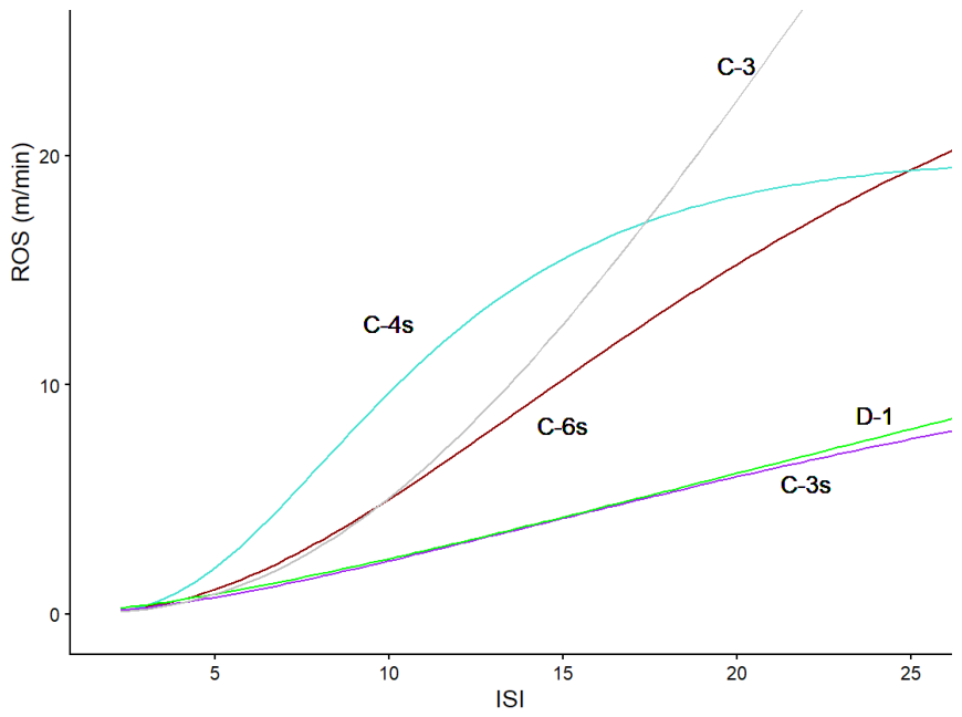
Figure 1. Comparison of surface fire rate of spread (ROS) models from the FBP System (C-6s, D-1) [11,16] (C-3s, C-4s). The full C-3 model (continuum of surface to crown fire ROS) is included for comparison purposes [11]. ISI refers to the Initial Spread Index.
Fire 09 00302 g001
Figure 2. Overview of rate of spread (ROS) of conifer fires, including surface and crown fire observations by open wind speed (WS10). Observations are organized by type of fire, with lines showing fitted linear trends. S, PC, and AC refer to surface, passive crown, and active crown fire types, respectively. The black line represents M20, the ‘20% WS10’ model for surface fire behaviour: R O S = 0.2 · W S 10 (ROS in m min−1; WS10 in km h−1).
Fire 09 00302 g002
Figure 3. Surface ROS observations by ISI and initial model fitting. Most symbols represent experimental fires except those with a black centre are wildfires. Colours indicate fuel type and fire characteristics as follows: JP—jack pine; S—black spruce or pine–spruce mix; OP—other pine; Decid—deciduous; PPDF-OC Ponderosa pine–Douglas-fir, original condition. Squares represent fires with significant torching (included in conifer models displayed but later removed). SFC indicates surface fuel consumption (kg m−2); observations lacking a measured SFC have a black outline and are plotted using mean overall SFC value (1.0 kg m−2). The lines represent linear (grey: Model 2) and quadratic (black: Model 3) ISI-based ROS models fitted to conifer observations (JP, S, OP). The green line is the FBP D-1 model.
Fire 09 00302 g003
Figure 4. Surface ROS observations by stand-adjusted ISI (ISIsa) from experimental fires (open symbols) and three wildfires (black centres) along with selected fitted models (labelled lines). Colours indicate fuel type: red—boreal conifer; blue—Ponderosa pine–Douglas-fir (PPDF) adjusted to ‘cured condition’ (CC); grey—PPDF in ‘original condition’ (OC); green—deciduous. Size indicates SFC, and black outlines indicate missing SFC values, displayed at SFC = 1.0 kg m−2. The M13 model line (red) is fitted only to the conifer observations, while the M9c (purple) and M11c (brown) lines are fitted to all fuel observations except OC PPDF. M19 (black) is only fitted to OC PPDF observations. Diamond and triangle shapes outline the highest-influence observations within M13 and M11c models, respectively, based on jackknife resampling. M9c lines are shown at SFC = 0.75 kg m−3 (dashed) and SFC = 3.0 kg m−3 (dotted), as indicated.
Fire 09 00302 g004
Figure 5. Boreal conifer surface fire observations by ISI and ROS, including both training and validation data, along with select model predictions. Overlapping observations were jittered by up to 0.1 m min−1 for clarity. The M16 model (brown lines) uses WS10 and mcFFMC as predictors rather than ISI; consequently, it is shown for both FFMC = 89 and FFMC = 92 conditions, as indicated. Grey shading indicates model extrapolation, beyond the range of data, where predictions diverge widely.
Fire 09 00302 g005
Table 1. Model numbers (M), predicted spread rate and evaluation metrics for a subset of fitted and predetermined models. See text for dataset descriptions. Formulae include 10-meter wind speed (WS10), initial spread index (ISI), stand-adjusted ISI (ISIsa), surface fuel consumption (SFC, kg m−2), litter moisture content estimated from the Fine Fuel Moisture Code (mcFFMC), and stand-adjusted model (mcsa), and fuel type (FT) variables. Predicted ROS (m min−1) is shown for three ISI or ISIsa levels; models without ISI/ISIsa are calculated with the following constants: FFMC 91 (M1, M5, M20), SFC of 1.0 kg m−2 (M9), and ‘conifer’ fuel type (M18c). Models 12–13, 18c include additional terms: m = 0.15, i = 10 (AGG), i = 13 (BOCON), for aggregated (AGG) and boreal conifer (BOCON) dataset models. Models M9c and M18c include estimated ‘fully cured’ condition ROS for 8 Ponderosa pine–Douglas-fir (PPDF) fires, while M19 is only fitted to those fires in their ‘original curing’ condition. Evaluation metrics include root mean squared error (RMSE, m min−1), mean absolute error (MAE, m min−1), mean absolute percentage error (MAPE, proportion), Efron’s R-squared (ER2), and Akaike’s Information Criterion (AIC). The predefined functions (not fitted) consist of the C-3s, C-4s, C-6s models, which were evaluated against the 53 BOCON observations; the D-1 model, tested against the 32 deciduous observations; and 20% WS10 model, tested against original 67 original conifer (CON) observations. For model estimates and statistics, see Appendix B.
Predicted ROS (m/min)Evaluation Metrics
Model
Number
FormulaNDatasetISI = 5ISI = 10ISI = 15RMSEMAEMAPEER2AIC
1β0 + WS1067CON0.93.54.81.591.120.7770.325257.9
3β1 · ISI258BOCON00.72.86.41.300.9460.6670.604199.0
5β1 · WS10253BOCON0.53.76.41.531.010.6990.450199.3
7β1 · ISI2 + β2 · sqrt(SFC) 80AGG1.01.93.51.270.8000.5620.607270.9
9cβ1 · ISIsa2 + β2 · sqrt(SFC)80AGG1.02.13.91.280.9030.5940.649272.7
12(m · ISI + i) · (1 − exp(−b · ISI)c)53BOCON0.32.66.71.050.8330.6290.742161.2
13(m · ISIsa + i) · (1 − exp(−b · ISIsa)c)53BOCON0.32.35.51.120.8900.6580.704168.4
16a · WS10b · exp(c · mcFFMC)53BOCON0.32.96.80.9520.7720.6000.786153.2
17a · WS10b · exp(c · mcsa)53BOCON0.42.95.91.020.7640.5740.755160.5
18c(m · ISI + i) · (1 − exp(−b · ISI)c +
d · PPDF + e · DECID)
93AGG0.72.54.81.380.9850.6560.618333.4
19β1 · ISIsa8PPDF0.61.21.80.8750.6970.370−1.5424.6
2020% WS1067CON1.23.44.41.601.0850.8760.370-
C-3s---0.72.34.2-0.8840.5880.555-
C-4s---2.09.715.5-4.4193.703−5.349-
C-6s---1.15.010.2-1.6701.482−0.044-
D-1---0.92.44.2-1.2970.9880.543-
Table 2. Model evaluation metrics for the validation dataset (N = 26). MAE is mean absolute error (m min−1), RMSE is root mean squared error (m min−1), MAPE is mean absolute percent error (proportion) and MBE is mean bias error (m min−1).
ModelMAERMSEMAPEMBE
M121.2021.670.779−0.121
M161.1741.570.797−0.045
M201.1891.411.1480.908
Table 3. Expected model accuracy for Models M12, M16, M20, and M9c, based on mean and 90th quantile over- and under-predictions for ISI or ISIsa < 11 and >11 classes (training data), or the validation dataset. MAE, Q90AE, MAPE, and Q90APE are Mean Absolute Error (m min−1), 90th quantile Absolute Error (m min−1), Mean Absolute Percent Error, and 90th quantile Absolute Percent Error, respectively.
ISI/ISIsaPredictionMAEQ90AEMAPEQ90APE
ModelDataset m min−1m min−1%%
M12Training < 11Over0.781.3393178
(ISI) Under0.741.594983
Training > 11Over1.162.0370151
Under1.741.942125
Validation 1.203.1278123
M16Training < 11Over0.761.5489205
(WS10, Under0.751.584983
mcFFMC)Training > 11Over0.811.234488
Under1.041.461523
Validation 1.172.980122
M20Training < 11Over1.01.9128270
(WS10) Under0.490.962142
Training > 11Over0.450.572223
Under4.36.325160
Validation 1.192.06115123
M9cTraining < 11Over0.571.0682166
(ISIsa, FT) Under0.771.733360
Training > 11Over1.43.1263134
Under3.063.754152
Table 4. Summary of recommended sROS models with their inputs, suggested use, and constraints. See main text for abbreviations.
ModelInputsSuggested PurposeConstraints
M9cISIsa, SFCContrast FC, stand structure across fuel typesMay overpredict under high-danger conditions; requires mcsa and SFC inputs
M11cISIsaGeneral stand-adjusted ROS prediction across various fuel typesRequires mcsa inputs
M12ISISimple model for boreal conifer fuelsNo stand structure influence
M13ISIsaSimple stand-adjusted model for boreal conifer fuelsRequires mcsa inputs
M16mcFFMC, WSMost accurate model for conifer stands in low–moderate-danger conditionsMay overpredict under high-danger conditions; no stand structure influence
M17mcsa, WSMost accurate stand-adjusted model for conifer stands in low–moderate-danger conditionsMay overpredict under high-danger conditions; requires mcsa inputs
M18cISI, FTContrast between conifer, deciduous, cured PPDF fuelsCured PPDF predictions based on untested assumptions; no stand structure influence other than FT
M19ISISimple linear model for moist-condition PPDF standsBased on small dataset; likely to underpredict under high-danger conditions; no stand structure influence
M20WSSimple heuristic model for rapid field useMay overpredict under moist fuel conditions and underpredict under dry fuel conditions; no stand structure influence
Disclaimer/Publisher’s Note: The statements, opinions and data contained in all publications are solely those of the individual author(s) and contributor(s) and not of MDPI and/or the editor(s). MDPI and/or the editor(s) disclaim responsibility for any injury to people or property resulting from any ideas, methods, instructions or products referred to in the content.