Spatial Chromatic Instability: A Lightweight Feature Extraction Technique for Wildfire Detection

Abstract

Spatial chromatic instability is currently one of the most robust methods for improving solutions proposed for image-based fire detection systems. Real flames exhibit erratic, turbulent local color variations, providing a more reliable discriminative signal than global color information alone, especially in visually ambiguous non-fire situations. This study proposes a generalizable feature representation based on the Spatial Chromatic Instability Index (ICCS) to measure local RGB variations (ICCS_R, ICCS_G, ICCS_B, and ICCS_T). Two public datasets comprising both fire image files and non-fire imagery were used. The Hilbert–Schmidt Independence Criterion (HSIC) and Silhouette coefficient analysis were used to quantify the statistical dependence between feature sets and the resulting cluster separation. To evaluate the practical discriminatory performance of spatial chromatic instability, three classifiers, i.e., Logistic Regression, Linear SVM, and Random Forest, were employed. To verify the proposed approach’s effectiveness, three deep learning models, Swin Transformer, MobileViT, and ViT-Base-16, were also employed for cross-checking. Performance metrics demonstrated that integrating ICCS features into global color features improved classification. Logistic Regression performed best overall on the Kaggle dataset when local ICCS features were included, achieving an accuracy of 0.935 and an F1-score of 0.958. For the Mendeley dataset, Linear SVM achieved an accuracy of 0.862 and an F1-score of 0.881. The ICCS is a robust, easy-to-understand, and fast approach for identifying fires. It has real potential in early warning systems, mainly due to its limited requirements for computing power.

1. Introduction

As of 31 March 2026, the European Forest Fire Information System reports that wildfires have burnt 54,572 hectares of land across the European Union. Since the start of the year, there have been 486 fires that have each damaged more than 30 hectares of land [1]. In 2025, wildfires killed more than 1 million hectares of vegetation in the European Union, making it one of the worst fire seasons since records began in 2006 [2]. Data from the Joint Research Centre indicate a rise in fire frequency and extent across southern and central Europe [3]. These fires are also burning longer and causing more damage [4]. These findings indicate the need to develop automated early-detection systems capable of rapidly and accurately identifying fires in images. Early fire detection can mitigate hazards by reducing reaction times and preventing the spread of flames.

Fire exhibits unique visual properties, including rapid spatial changes in hue from yellow to orange to red. It also experiences brightness fluctuations between a hot core and cooler edges. The irregular spatial texture lacks fixed boundaries and has high-frequency chromatic gradients due to turbulence. These properties are quite different from those of static red or orange objects, traffic signs, clothing, sunset lighting, or wood. Conventional fire-detection approaches frequently rely on global color descriptors such as histogram statistics, color moments, or threshold-based segmentation. While these features effectively capture the overall color distribution of an image, they often struggle in visually ambiguous scenes such as sunsets, artificial lighting, autumn foliage, reflections, and brightly illuminated objects, which may exhibit color distributions similar to those of flames. Highly reflective red/orange autumn leaves, bare soil, or reddish sunset lighting hitting clouds and haze can mimic the exact chromatic signatures of flames and smoke. Fires and smoke are highly dynamic and non-uniform. Global features treat the image as a flat color distribution, ignoring the internal spatial structure. Because global descriptors summarize information across the entire image, they may fail to distinguish genuine fire regions from non-fire regions that share comparable chromatic characteristics.

Real flames exhibit highly irregular spatial variations caused by combustion dynamics, turbulence, and fluctuating illumination. These variations manifest as rapid local changes in RGB values that are not adequately represented by global color statistics. The proposed Spatial Chromatic Instability Index (ICCS) addresses this limitation by quantifying the local chromatic variability within small spatial neighborhoods. Rather than describing only the overall color composition of an image, the ICCS captures the unstable and heterogeneous color patterns that characterize fire regions. Consequently, the ICCS provides complementary information to global color descriptors and improves discrimination between fire and visually similar non-fire scenes, rather than introducing a sophisticated feature fusion architecture.

This study aims to investigate whether local chromatic instability offers a unique visual characteristic for fire detection beyond traditional global color features. Our goal is not to develop a universal local descriptor. To evaluate the effectiveness of the proposed approach, two types of features are analyzed: (i) global chromatic descriptors based on Otsu segmentation and HS-type statistics, and (ii) ICCS features, which quantify local chromatic instability. In this perspective, a detection approach capable of accurately and swiftly identifying flames within any image is proposed. The main contributions of this study are as follows:

(i) We propose a novel framework based on the Spatial Chromatic Instability Index (ICCS) to assess local variations across the RGB channels for fire detection. The ICCS is computed over a 5 × 5 sliding window to better capture the unstable, irregular patterns typical of real fires.

(ii) We conducted a comparative analysis using the Hilbert–Schmidt Independence Criterion (HSIC) with various kernels and the Silhouette coefficient to demonstrate the complementary relationship between global and local descriptors. Each kernel captures only local information within its immediate area of effect, so this approach expands the comparison.

(iii) We evaluated the performance of several machine learning classifiers (Logistic Regression, SVM, Random Forest) as baseline models, in distinguishing between fire and non-fire images when local and global features are considered. We identified the most effective classifier for complex fire detection tasks. To verify the proposed approach’s effectiveness, three deep learning models, Swin Transformer, MobileViT, and ViT-Base-16, were also employed for cross-checking.

Early image-based fire detection methods relied primarily on handcrafted color and texture descriptors combined with rule-based classification schemes. These approaches exploited the characteristic red–orange–yellow appearance of flames, but their performance was often limited by illumination changes, background clutter, and the presence of fire-like objects.

One important research direction focuses on gradient-based features, which describe spatial color transitions and edge information. Liping et al. [5] introduced Gradient Features to characterize color changes across RGB channels and combined them with Support Vector Machines and decision trees for flame recognition. Their method improved discrimination between flames and visually similar objects such as fog, candlelight, and colored clothing. Liang et al. [6] further combined color segmentation, multidimensional flame descriptors, and Random Forest feature selection with a neural network classifier. Although gradient-based descriptors capture local color transitions, they primarily emphasize edge variations and do not explicitly quantify the irregular chromatic fluctuations produced by flame turbulence. Feature selection methods and model adaptation to regional contexts are further key factors for improving RGB-image-based classification systems, providing a robust foundation for the development of effective forest fire prediction systems [7,8].

The vision-based fire detection research direction embeds nonlinear visual perception and illumination constraints to distinguish actual flames from dynamic environmental distractors. Kikuta et al. [9] proposed a daytime smoke detection method based on the optical flow variance and HSV color features. They acknowledge that images often suffer from nonlinear visual perception and illumination dependency, so their approach focuses on color discrimination to exclude non-smoke areas. Both saturation and value components were employed to narrow down potential smoke areas. To ensure models’ reliability, the statistical dependence between extracted feature representations and ground-truth fire events is assessed using various methods. Hu et al. [10] used the HSIC to test the statistical dependence between two random variables. Their experiment utilized the forest fire data from the UCI repository and varied the associated kernel function. By maximizing the HSIC-based nonlinear dependency measure, false positives are suppressed while maintaining high detection sensitivity across varying environmental contexts.

Another line of research investigates fractal-based features, which characterize the geometric complexity and self-similar structure of image textures. Moldovanu et al. [11] demonstrated that combining surface fractal dimensions with statistical color descriptors improves classification performance by integrating global color information with local texture characteristics. While fractal descriptors effectively represent spatial complexity, they are designed to model texture roughness rather than the unstable color dynamics that are characteristic of real flames.

Machine algorithms were used for feature selection and classification. Caiado et al. [12] demonstrated that classical machine learning models can predict wildfire occurrence based on meteorological and geographical data. They evaluated the effectiveness of three classification models, i.e., Logistic Regression, Random Forest, and XGBoost, for wildfire prediction. The results showed that shrubland fires are the most predictable, while fires in settlements and agricultural areas are more difficult to estimate. Ali and Kareem [13] demonstrated the effectiveness of the Random Forest algorithm for forest fire prediction using environmental features derived from the UCI Forest Fires dataset. The proposed model achieved an accuracy of 93.6%, outperforming other widely used machine learning algorithms like SVM, ANN, KNN, Naive Bayes, and Decision Trees.

Recent advances in computer vision have increasingly adopted deep learning architectures for fire and smoke detection. Fireframe [14], based on YOLO and MobileNet variants, and CCi-YOLOv8n [15] demonstrated strong detection performance in challenging environments. Comprehensive reviews have also highlighted the effectiveness of convolutional and transformer-based models for fire and smoke recognition [16]. However, these methods typically require large training datasets, substantial computational resources, specialized hardware, and longer inference times, which may limit their deployment in low-power edge devices and real-time early-warning systems.

Despite these advances, a gap remains between global color descriptors, gradient-based features, fractal-based texture representations, and computationally demanding deep learning approaches. Existing methods generally capture global chromatic distributions, local edge information, texture complexity, or high-level learned representations. However, they do not explicitly model chromatic instability, i.e., the rapid and irregular spatial fluctuations in RGB values caused by flame turbulence. Such instability is a distinctive visual characteristic of fire and provides complementary information not fully captured by gradient or fractal descriptors.

To address this limitation, the present study introduces the ICCS, a lightweight feature representation that quantifies local RGB variability within small spatial neighborhoods. Unlike gradient-based approaches that measure color transitions and unlike fractal-based methods that characterize texture complexity, the ICCS directly measures the instability of chromatic patterns generated by flames. The proposed descriptor is computationally efficient, interpretable, and suitable for real-time applications, while maintaining competitive performance relative to substantially more complex deep learning solutions.

2. Methodology

An effective fire detection approach starts by identifying features that genuinely reflect how flames appear in real-world conditions. The first step in this work was to separate potential fire regions from the background. This was achieved by applying adaptive Otsu thresholding to each RGB channel. At the same time, global color information was captured through Histogram Spread (HS), which provides an overall view of the pixel intensity distribution. However, global descriptors alone have severe limitations, particularly in scenes where non-fire elements can visually resemble flames. To overcome these issues, the second research step introduced a set of features that focus on local color variations. The framework used the Spatial Chromatic Instability Index (ICCS) to analyze how RGB values fluctuate within small neighborhoods. The ICCS components (ICCS_R, ICCS_G, ICCS_B) and a combined measure (ICCS_T) were computed over a 5 × 5 sliding window to better capture the unstable, irregular patterns typical of real fires.

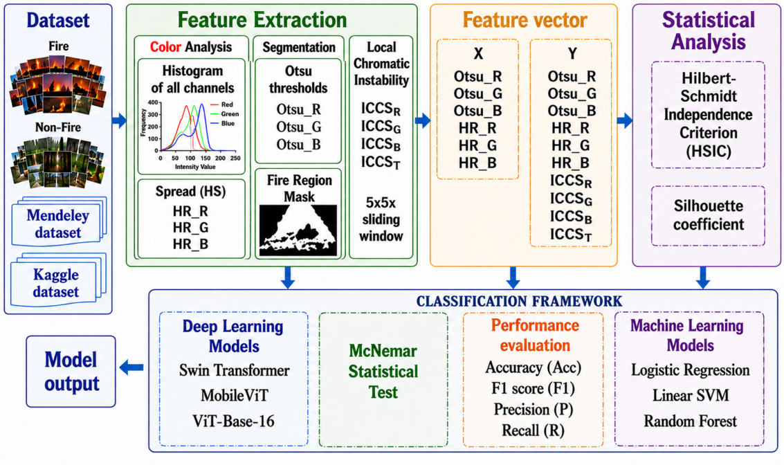
Then, how well these features separate fire and non-fire classes was studied using the Hilbert–Schmidt Independence Criterion (HSIC) and the Silhouette coefficient. To further assess the performance of the proposed method, both global and local color features were used to train baseline models, including Logistic Regression, Linear SVM, and Random Forest. Also, three deep learning models—Swin Transformer, MobileViT, and ViT-Base-16—were used to cross-check the proposed approach’s utility. Any improvements to the deep learning model’s architecture are beyond the scope of the current research. The classification performance was evaluated using standard metrics such as overall accuracy, precision, recall, F1-score, and ROC curves. The performance metrics were separately computed for fire and non-fire data. These metrics assess how well classifiers perform in fire detection. Missing a positive instance is dangerous, and the cost of false negatives is high. The proposed framework is depicted in Figure 1.

2.1. Mathematical Approach

2.1.1. The Color Histogram

The color histogram describes the color content of an image and quantifies the number of occurrences of each color [17]. For a given RGB image, let L be the intensity levels in the range [0, 1, 2, …, L − 1][0, 1, 2, …, L − 1][0, 1, 2, …, L − 1]. The probability distribution is as follows:

$$p_i^c={\displaystyle \frac{h_i^c}{N}},\mathrm{ }{\displaystyle \sum _{i=0}^{L-1}}{p}_i^c=1$$

(1)

where i is a specific level of intensity in the range $\{0\le i\le L-1\}$ for the color component $C=\{R,G,B\}$, N is the total number of pixels in the image, and $h_i^c$ is the number of pixels for the intensity level i in the component C.

2.1.2. Otsu Thresholding

The Otsu method is a discriminant analysis between two groups of pixels based on a threshold t that maximizes the separation between the two classes [18]:

$${\sigma }_B^2(t)={{\omega }_0{\omega }_1\left({\mu }_0-{\mu }_1\right)}^2$$

(2)

where t is the selected threshold; ${\omega }_0, {\omega }_1$ are the class probabilities; and ${\mu }_0, {\mu }_1$ denote the class means. The optimal threshold is obtained by maximizing the between-class variance to ensure maximum separability between the background and foreground classes.

Otsu thresholding is applied independently to each RGB channel: [$T_R, T_G, T_B$] yielding three binary masks: $M_R=\left(R>T_R\right)$, $M_G=\left(G>T_G\right)$, and $M_B=\left(B>T_B\right)$. The final fire-region mask is obtained using logical intersection, $\mathsf{\Omega }=M_R\cap \overline{M_G}\cap \overline{M_B}$. $\overline{M_G}$ and $\overline{M_B}$ denote the complements of the green and blue masks, respectively. This operation was selected because fire pixels are typically characterized by a dominant response in the red channel and comparatively lower responses in the green and blue channels. Compared with union-based approaches, the proposed intersection rule employed a more conservative segmentation, reducing false positives caused by bright non-fire regions or isolated high-intensity responses in individual color channels.

2.1.3. Histogram Spread (HS)

The data displayed in color histograms can be analyzed using histogram equalization methods for each color channel (HS), defined as follows [19]:

$$HS={\displaystyle \frac{‖IQR‖}{‖R‖}}$$

(3)

where IQR is the distance between the 1st and the 3rd quartile, R is the range of monochromatic pixels, and $‖·‖$ denotes the L2 norm that is also known as the Euclidean norm or length.

2.1.4. Spatial Chromatic Instability Index (ICCS)

The local chromatic instability is computed by combining the local standard deviation of one channel with the absolute differences between channel-wise standard deviations. For each pixel (x, y) belonging to the segmented fire region:

$$ICCS={\displaystyle \frac{1}{\left|\mathsf{\Omega }\right|}}\sum _{\left(x,y\right)\in \mathsf{\Omega }}\left({\sigma }_R\left(x,y\right)+\left|{\sigma }_R-{\sigma }_G\right|+\left|{\sigma }_G-{\sigma }_B\right|\right)$$

(4)

where $\mathsf{\Omega }$ denotes the binary fire mask obtained via Otsu-based segmentation; ${\sigma }_R\left(x,y\right)$, ${\sigma }_G\left(x,y\right)$, and ${\sigma }_B\left(x,y\right)$ are computed within the same k×k neighborhood centered on pixel (x, y). All three channels were evaluated over an identical spatial support region. The ICCS combines color information with spatial dynamics to differentiate fires and fire-like objects.

No additional weighting coefficients were introduced because the objective of the ICCS is to preserve the natural contribution of each RGB channel and to emphasize chromatic instability arising from inter-channel variability. Preliminary experiments showed that introducing manually selected weights did not consistently improve discrimination performance and increased the number of tunable parameters. Consequently, an unweighted formulation was adopted to maintain simplicity, interpretability, and computational efficiency.

The descriptor is averaged over all pixels belonging to the segmented fire region:

$$ICCS={\displaystyle \frac{1}{\left|\mathsf{\Omega }\right|}}\sum _{\left(x,y\right)\in \mathsf{\Omega }}ICCS(x, y)$$

(5)

This averaging operation naturally normalizes the descriptor with respect to region size. Additional normalization by the number of channels was not applied because the descriptor is used comparatively across all images under the same formulation and scale.

Algorithm 1 summarizes the computation of the ICCS. Starting from an RGB image, Otsu thresholding is applied independently to each color channel to obtain a fire-region mask Ω. For every pixel belonging to Ω, local standard deviations are computed within a (5 × 5) sliding window. These local statistics are then combined according to Equation (4) to obtain pixel-wise chromatic instability values, which are finally averaged over the segmented region to produce the channel-specific descriptors ((ICCS_R), (ICCS_G), (ICCS_B)) and the overall instability measure (ICCS_T).

Algorithm 1: ICCS-Based Fire Detection and Classification Framework
Input: RGB fire and non-fire images Output: Fire/Non-fire classification
{Step 1} Load RGB images from the Mendeley and Kaggle datasets. {Step 2} Separate the RGB image into the R, G, and B channels. {Step 3} Extract global color features:      - Otsu_R, Otsu_G, Otsu_B      - HS_R, HS_G, HS_B {Step 4} Apply Otsu thresholding independently to the R, G, and B channels. {Step 5} Generate binary masks: MR, MG, MB {Step 6} Generate the fire-region mask: M = MR ∪ MG ∪ MB {Step 7} Apply a 5 × 5 sliding window (Ω) over pixels belonging to M. {Step 8} Compute local standard deviation: σR, σG, σB {Step 9} Compute local chromatic instability descriptors:      ICCSR = mean(σR)      ICCSG = mean(σG)      ICCSB = mean(σB) {Step 10} Compute total chromatic instability:      ICCST = ICCSR + ICCSG + ICCSB {Step 11} Construct feature vectors:      X = [Otsu_R, Otsu_G, Otsu_B,         HS_R, HS_G, HS_B,	Y = [Otsu_R, Otsu_G, Otsu_B,      HS_R, HS_G, HS_B,         ICCSR, ICCSG, ICCSB, ICCST] {Step 12} Analyze feature relevance and separability:      - Normalized HSIC      - Silhouette coefficient {Step 13} Train machine learning models:      - Logistic Regression      - Linear SVM      - Random Forest {Step 14} Train deep learning models:      - MobileViT      - Swin Transformer      - ViT-Base-16 {Step 15} Evaluate models using:      - Accuracy      - Precision      - Recall      - F1-score {Step 16} Compare classifiers using the McNemar statistical test. {Step 17} Select the best-performing model and report final results.

2.1.5. The Silhouette Index

The Silhouette index S(i) for object i belonging to a cluster is given as follows [20]:

$$S(i)={\displaystyle \frac{b\left(i\right)-a\left(i\right)}{max\left\{a\left(i\right),\mathrm{ }b\left(i\right)\right\}}}$$

(6)

where a(i) is the average dissimilarity of the i-object from the rest of the objects in the same cluster; b(i) is the minimum of the average dissimilarity of the i-object from the rest of the objects in the neighbor cluster. S(i) ranges from −1 to +1. An S(i) close to +1 indicates a quality clustering, whilst a value close to −1 indicates a worse clustering. S(i) = 0 indicates that the analyzed objects are dispensed to another neighbor cluster.

2.1.6. Hilbert–Schmidt Independence Criterion (HSIC)

The HSIC is a kernel method used to evaluate the statistical dependence between various random variables in nonlinear dependence measures [21]. Lower HSIC values (close to zero) indicate greater independence. For two vectors, ${\left\{x_i\right\}}_{i=1}^n$ and ${\left\{y_i\right\}}_{i=1}^m$, and associated kernels $k(x_i, x_j)$ and $l(y_i, y_j)$, the following kernel matrices are defined $K_{ij}=k(x_i, x_j)$ and $L_{ij}=(y_i, y_j)$. The HSIC kernel distance covariance is as follows:

$$HSIC \left(X, Y\right)={\displaystyle \frac{1}{n^2}}trace (KHLH)$$

(7)

where H denotes the centering matrix $H=\mathcal{I}-{\displaystyle \frac{1}{n}}\mathbb{I}{\mathbb{I}}^T$. $\mathcal{I}$ is the identity matrix, $\mathbb{I}$ is a vector of ones, and ${\mathbb{I}}^T$ denotes the transpose of $\mathbb{I}$. Then, $HSIC \left(X, Y\right)=0$ if and only if X and Y are independent, ($X\perp Y)$. The empirical HSIC is computed as follows:

$$HSIC \left(X, Y\right)={\displaystyle \frac{1}{{(n-1)}^2}}trace (K_{X}H{L}_{Y}H)$$

(8)

The most utilized kernels are presented in

Table 1. Kernel selection and attributes.

RBF (Gaussian) kernel/radial basis functions	$k\left(x_i, x_j\right)=exp\left(-{‖x_i-x_j‖}^2/2{\sigma }^2\right)$	σ is the Gaussian kernel bandwidth controlling local similarity
Median heuristic kernel	$D_X=\left\{‖x_i-x_j‖/i<j\right\}$ ${\sigma }_X=median \left(D_X\right)$	Automatic bandwidth estimation robust to nonlinear data distributions
Multi-scale kernels-variant 1	$k\left(x, x^{\prime }\right)={\sum }_{q=1}^{Q}exp\left(-{‖x-x\prime ‖}^2/2{{\sigma }_q}^2\right)$ ${\sigma }_q=[{\displaystyle \frac{\sigma }{2}}, \sigma , 2\sigma ]$	${\sigma }_q$ is the Gaussian bandwidth at scale q Q is the total number of kernel scales used in HSIC computation
Multi-scale kernels-variant 2	$k\left(x, x^{\prime }\right)={\sum }_{q=1}^Q{w}_q exp\left(-{‖x- x\prime ‖}^2/2{{\sigma }_q}^2\right)$ $w_q=softmax{\alpha }_q$ Softmax of HSIC contributions: ${\alpha }_q={\displaystyle \frac{1}{{(n-1)}^2}}trace (K_{X,q}H{L}_{Y}H)$ $softmax{\alpha }_q={\displaystyle \frac{e^{{\alpha }_q}}{{\displaystyle {\sum }_{j=1}^k}{e}^{{\alpha }_k}}}$	$w_q$ is adaptive softmax-based kernel weights ${\alpha }_q$ adaptive scale parameters—automatically determined based on median heuristic

.

The HSIC analysis was supplemented with a normalized HSIC measure. The nHSIC was computed by applying the standard HSIC function to the dataset’s variables and then normalizing by the respective individual HSIC values of each variable:

$$nHSIC(X,Y)=\frac{HSIC\left(X,Y\right)}{\sqrt{HSIC\left(X,X\right)·HSIC\left(Y,Y\right)}}$$

(9)

The normalized nHSIC values provide a scale-independent assessment of statistical dependence and allow for more meaningful comparisons between the Kaggle and Mendeley datasets.

2.1.7. Statistical Tests

McNemar’s test examines differences in the sensitivity and specificity between two paired classifiers. This comparison helps determine which classifier performs better within the same dataset.

$${\chi }^2=\frac{{\left(\left|n_{01}-n_{10}\right|-1\right)}^2}{n_{01}+n_{10}}$$

(10)

where n₀₁ is the number of samples correctly classified only by the model A and misclassified by the compared baseline model B; n₁₀ is the number of samples correctly classified only by the compared baseline B classifier and misclassified by A. McNemar’s test, which measures disagreement between classifiers’ predictions, was used on the Mendeley and Kaggle datasets. The classifiers use both global color descriptors and an ICCS-enhanced feature representation.

2.1.8. Comparative Analysis with Baseline Models

To rigorously validate the robustness of the proposed approach, detailed benchmarking against established feature representations for global and local chromatic instability was conducted. This involves using Random Forest, Logistic Regression, and Linear SVM classifiers as baseline models. Logistic Regression offers a linear approach for the binary classification of fire occurrences. It is both interpretable and computationally efficient. Random Forest, an ensemble of decision trees trained on bootstrapped samples, demonstrates high predictive performance due to random feature selection at each node, which captures complex, nonlinear interactions and reduces overfitting. Linear SVM is highly efficient for high-dimensional, linearly separable data. It performs very well when the number of features is large.

Then, we compared the performance of the machine learning algorithms against three representative deep learning models: Swin Transformer (swin_tiny_patch4_window7_224 variant), MobileViT (mobilevit_s is the small variant of MobileViT), and ViT-Base-16 (vit_base_patch16_224 variant). This comparison was purely to cross-check the proposed approach’s utility and not to refine the deep learning models. The main advantage is the computational cost, which favors our approach. Before training, all these models underwent a two-step preprocessing process. First, RGB images were converted to the HSV color space, using the Hue (H) and Saturation (S) components to highlight specific fire regions. Then, the Otsu adaptive threshold method automatically segmented these areas. Before ICCS extraction, all images underwent Contrast Limited Adaptive Histogram Equalization (CLAHE) in the LAB color space. The RGB image was first converted to the LAB space. The luminance information (L channel) was separated from chromatic information (A and B channels). CLAHE was applied only to the luminance channel, and the image was subsequently converted back to RGB before ICCS computation. The CLAHE preprocessing was applied uniformly to all images in both datasets rather than selectively to low-contrast images. This ensured a consistent processing pipeline and avoided introducing image-dependent preprocessing decisions.

To evaluate the performance of the proposed method, the following metrics were computed [22]:

$$Recall(R)={\displaystyle \frac{TP}{TP+FN}}$$

(11)

$$Accuracy(ACC)={\displaystyle \frac{TP+TN}{TP+TN+FP+FN}}$$

(12)

$$Precision(P)={\displaystyle \frac{TP}{TP+FP}}$$

(13)

$$F_{1 score}={\displaystyle \frac{2·Precision·Recall}{Precision+Recall}}$$

(14)

where TP is true positive, FP is false positive, TN is true negative, and FN is false negative.

To evaluate the discriminative ability across different feature representations, we utilized the Receiver Operating Characteristic (ROC) curve, which represents the trade-off between the True Positive Rate (sensitivity) and False Positive Rate (1-specificity).

2.2. Datasets

To test the proposed method, we conducted experiments on two publicly available datasets, Kaggle [23] and Mendeley [24,25], both of which contain fire and non-fire images. Detailed information on these datasets is provided in

Table 2. Details about images used to extract V1 and V2 feature vectors, providing the number of negative samples/non-fire and of positive samples containing flames, smoke, or both.

Dataset	Type	Fire	Non-Fire	Total	Notice
Kaggle dataset— FIRE Dataset [23]	Images	755	244	999	It comprises a diverse collection of images that depict fire and smoke scenarios. The non-fire images contain forest, tree, grass, river, people, foggy forest, lake, animal, road, and waterfall.
Mendeley dataset— Forest Fire Dataset (Classification) [24,25]	Images	1672	1275	2947	The collection is made up of two groups of photos: the fire group, which shows forest fires (flames, smoke, and burned vegetation), and the non-fire group, which shows trees that have not been damaged, showing what natural ecosystems are usually like.

.

A total of 3946 images were used to extract X and Y feature vectors and create a new classification dataset for three machine learning algorithms. The data were acquired under various environmental conditions, including sunlight, clouds, fog, and different illumination scenarios such as reflections and red-colored objects. The resulting feature dataset was divided into training and test subsets using an 80:20 ratio.

3. Results

We propose a new approach to distinguishing between fire and non-fire instances, using features such as RGB channel histograms, histogram spread (HS_R, HS_G, HS_B), Otsu thresholds for each channel (Otsu_R, Otsu_G, Otsu_B), the fire region mask, and local chromatic instability indicators computed on 5 × 5 sliding windows (ICCS_R, ICCS_G, ICCS_B, ICCS_T). Two feature sets were used: X = [Otsu_R, Otsu_G, Otsu_B, HS_R, HS_G, HS_B] and Y = [Otsu_R, Otsu_G, Otsu_B, HS_R, HS_G, HS_B, ICCS_R, ICCS_G, ICCS_B, ICCS_T]. Because we could not fairly compare our proposed approach with other studies, we experimented on two different publicly available datasets.

Tests were conducted on a personal computer equipped with an Intel Core i3-4030U processor (1.90 GHz), 8 GB of RAM, and integrated Intel HD Graphics. The model was implemented in Python version 3.12.13 (Python Software Foundation, Wilmington, DE, USA) and using the open-source computer vision library, OpenCV version 4.13.0 (OpenCV Team, San Francisco, CA, USA).

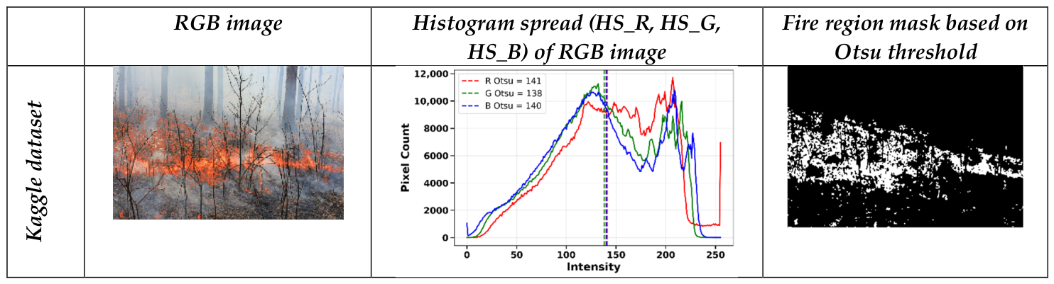
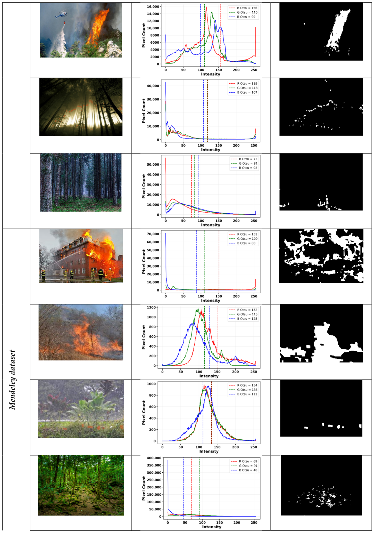
Figure 2 shows an example of global color analysis and segmentation. Fire images exhibit a dominant red channel distribution, moderately high green channel values, and moderately low blue channel values. Non-fire or fire-like objects have a more balanced, low-intensity distribution across channels. However, there is no rule for detection based on these criteria. The disadvantage of this approach is that luminance conditions vary across environments, making it difficult to extract color-based descriptors for different background environments.

The ICCS descriptor relies on local standard deviations computed within a sliding window. A window size of (5 × 5) pixels was selected as a compromise between noise sensitivity and spatial averaging. Smaller windows, such as (3 × 3), are highly sensitive to local noise and produce unstable estimates of channel standard deviation. Larger windows, such as (7 × 7), smooth fine flame structures, and reduce sensitivity to rapid chromatic variations caused by combustion turbulence. To justify the choice of ICCS neighborhood size, an ablation study was conducted using four window sizes (3 × 3, 5 × 5, 7 × 7, and 9 × 9) on the Kaggle dataset. Logistic Regression and Linear SVM classifiers were employed with ICCS features (

Table 3. Classification performance obtained for different ICCS neighborhood sizes (Ω = 3 × 3, 5 × 5, 7 × 7, and 9 × 9) on the Kaggle dataset. For each neighborhood size, the best-performing classifier is reported. Accuracy, F1-score for the fire class, and F1-score for the non-fire class are presented.

Window	Best Model	Accuracy	F1 (Fire)	F1 (Non-Fire)
3 × 3	Logistic Regression + ICCS	0.915	0.945	0.817
5 × 5	Logistic Regression + ICCS	0.935	0.958	0.853
7 × 7	Logistic Regression + ICCS	0.930	0.954	0.851
9 × 9	Linear SVM + ICCS	0.930	0.955	0.848

). The results demonstrated that the 5 × 5 neighborhood achieved the best overall classification performance, with 0.935 accuracy and F1-scores of 0.958 and 0.853 for the fire and non-fire classes, respectively. Smaller neighborhoods (3 × 3) were more sensitive to local noise and produced lower performance, while larger neighborhoods (7 × 7 and 9 × 9) slightly reduced discriminative power due to the excessive spatial smoothing of local chromatic variations.

The results indicate that the 5 × 5 neighborhood provides the best balance between local-detail preservation and statistical stability, with the best trade-off between local sensitivity and robustness. Consequently, all experiments reported in this study employed a 5 × 5 sliding window.

We analyzed the dependency between X and Y feature groups using the HSIC method. Three different kernel functions were selected to measure attributes in different spaces.

Table 4. HSIC (X, Y) results for regular RBF (Gaussian), median heuristic, and adaptive multi-scale kernels. If X and Y are strongly dependent (i.e., redundant features), HSIC (X, Y) takes a large value.

Dataset	Number of Features	RBF (Gaussian) Kernel	Median Heuristic Kernel	Multi-Scale Kernels
Kaggle	X (5994)	0.003142	0.003265	0.000915
	Y (8991)
Mendeley	X (17,682)	0.019876	0.026085	0.006909
	Y (26,523)

quantifies the statistical dependence between the two feature groups.

The two sets are statistically independent. This reduced reliance suggests that chromatic instability ICCS features complement global descriptors rather than being captured by them. Multi-scale kernels are often used to make the HSIC more robust to the choice of kernel bandwidth. Data-adaptive weight kernels decrease descriptor group redundancy and separate complementary information. Multi-scale kernels are most suitable for complex nonlinear feature interactions in forest fire detection and classification. To further explore the independence of chromatic instability descriptors, an additional weighted, channel-wise HSIC analysis was performed using adaptive softmax weighting (

Table 5. Channel-wise weighted HSIC results for ICCS features.

Dataset	Channel	HSIC Score	Adaptive Weights
Mendeley	ICCSR	0.012254	0.333409
	ICCSG	0.012114	0.333363
	ICCSB	0.011710	0.333228
Kaggle	ICCSR	0.001907	0.333103
	ICCSG	0.002362	0.333255
	ICCSB	0.003524	0.333642

).

Once more, the channel-wise HSIC with adaptive softmax weighting reveals that X and Y feature groups are very weakly related. The balanced adaptive weight shows the durability and stability of the multi-scale kernel architecture.

Furthermore, the normalized HSIC analysis revealed a moderate statistical dependency between ICCS and global color descriptors on the Mendeley dataset, with nHSIC values ranging from 0.432 to 0.603 (

Table 6. Channel-wise normalized nHSIC and adaptive weights for ICCS features.

Dataset	Channel	Normalized HSIC	Adaptive Weights
Mendeley	ICCSR	0.602667288	0.35630068
	ICCSG	0.565410651	0.343270356
	ICCSB	0.432103639	0.300428964
Kaggle	ICCSR	0.105658447	0.345343011
	ICCSG	0.062911995	0.33089189
	ICCSB	0.041138538	0.323765099

). In contrast, substantially lower NHSIC values were obtained for the Kaggle dataset (0.041–0.106), indicating that ICCS descriptors provide largely complementary information to Otsu and histogram-based features. Across both datasets, the red channel exhibited the highest dependency scores, confirming its dominant role in characterizing fire-related chromatic variations.

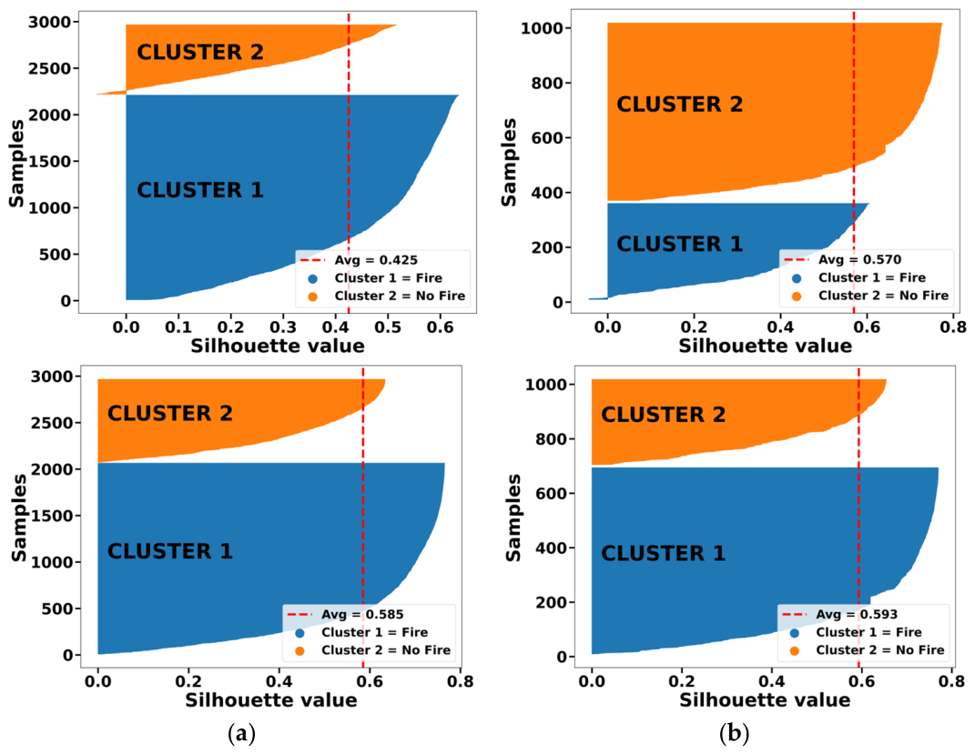
Figure 3 and Figure 4 present the results of the Silhouette analysis. This analysis evaluates the effectiveness of the chosen features in distinguishing data and, consequently, assesses their reliability in categorization. As illustrated in Figure 3, the Silhouette analysis indicates that ICCS features significantly improve class selectivity. The combined ICCS metric provides an average Silhouette index of 0.59 for the Kaggle dataset and of 0.60 for the Mendeley dataset, suggesting that the clusters are more compact and there is less overlap between the fire and non-fire samples. The samples are correctly separated into individual channels.

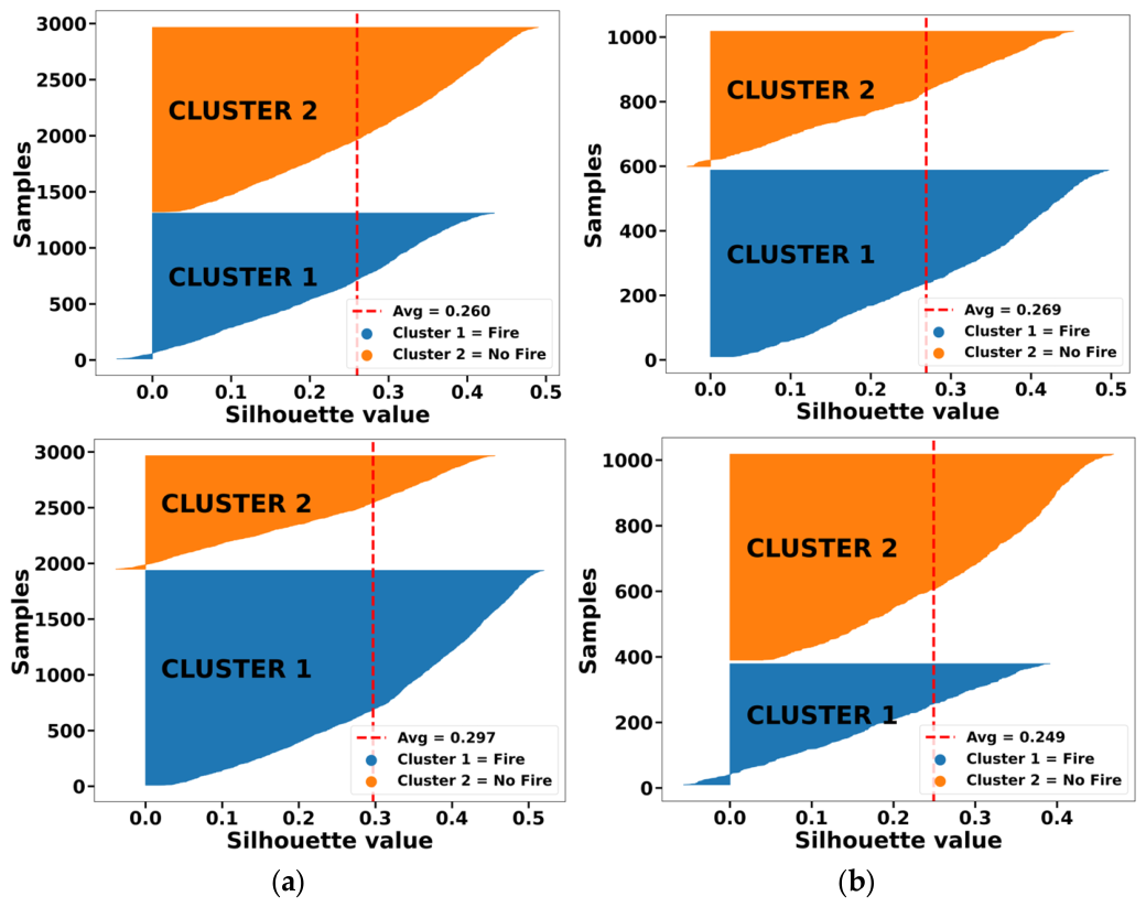
Figure 4 demonstrates that global color features (X) exhibit a lower ability to separate fire and non-fire samples. The average Silhouette scores for both datasets are around 0.26, indicating that the clusters are quite comparable. Combining global color and ICCS features yields only a slight improvement, with the average Silhouette index values remaining below 0.30. This suggests that a global color-based approach is not effective for class separation. The likelihood of errors in distinguishing non-fire instances that visually resemble those affected by flames is higher.

To verify the impact of ICCS features on model performance, we trained and tested various models using multiple color representations. The X and Y high-dimensional feature vectors provide a robust foundation for subsequent classification tasks (detailed in Figure 1). They form a new dataset for fire/non-fire classification. By using identical training and validation datasets, we ensured a fair comparison of each model’s classification performance.

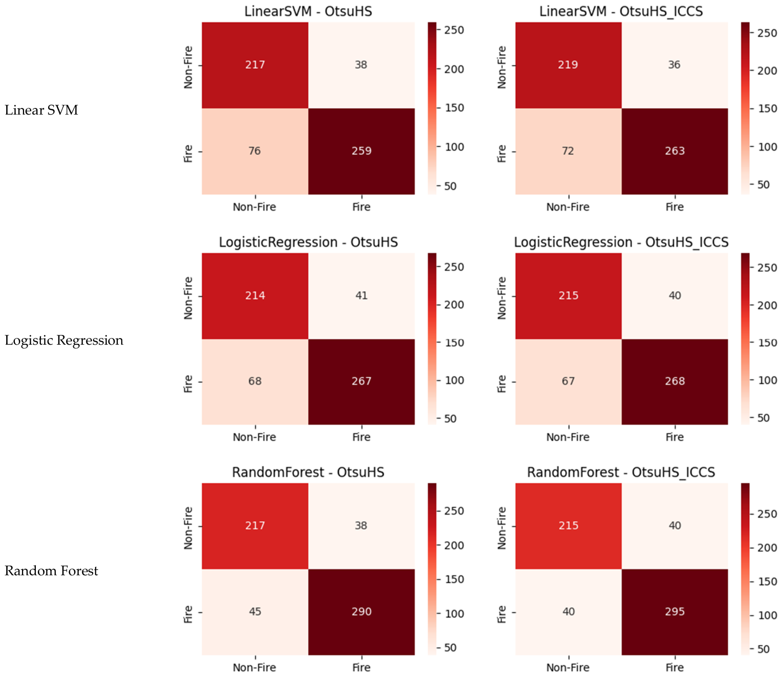
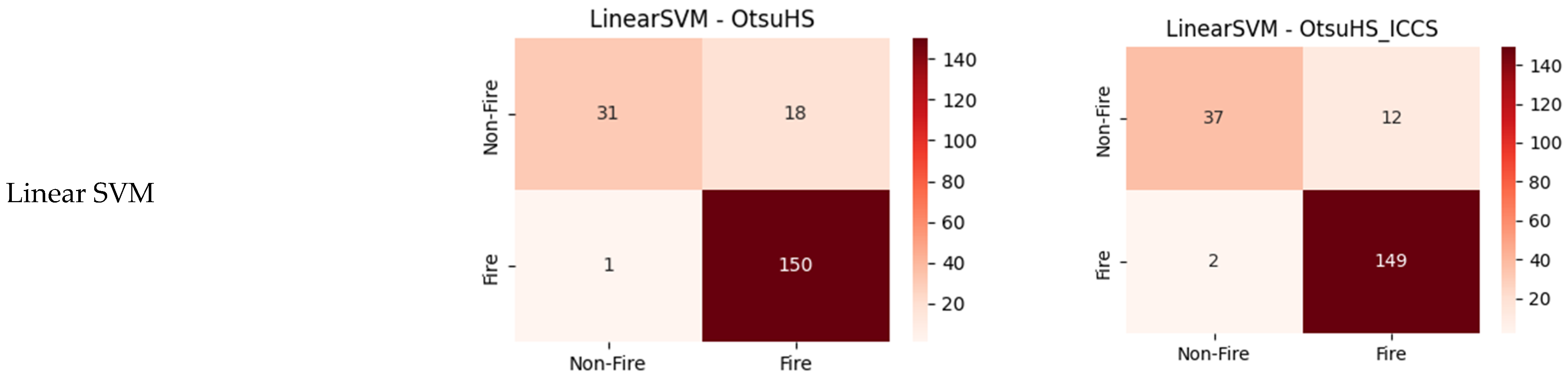
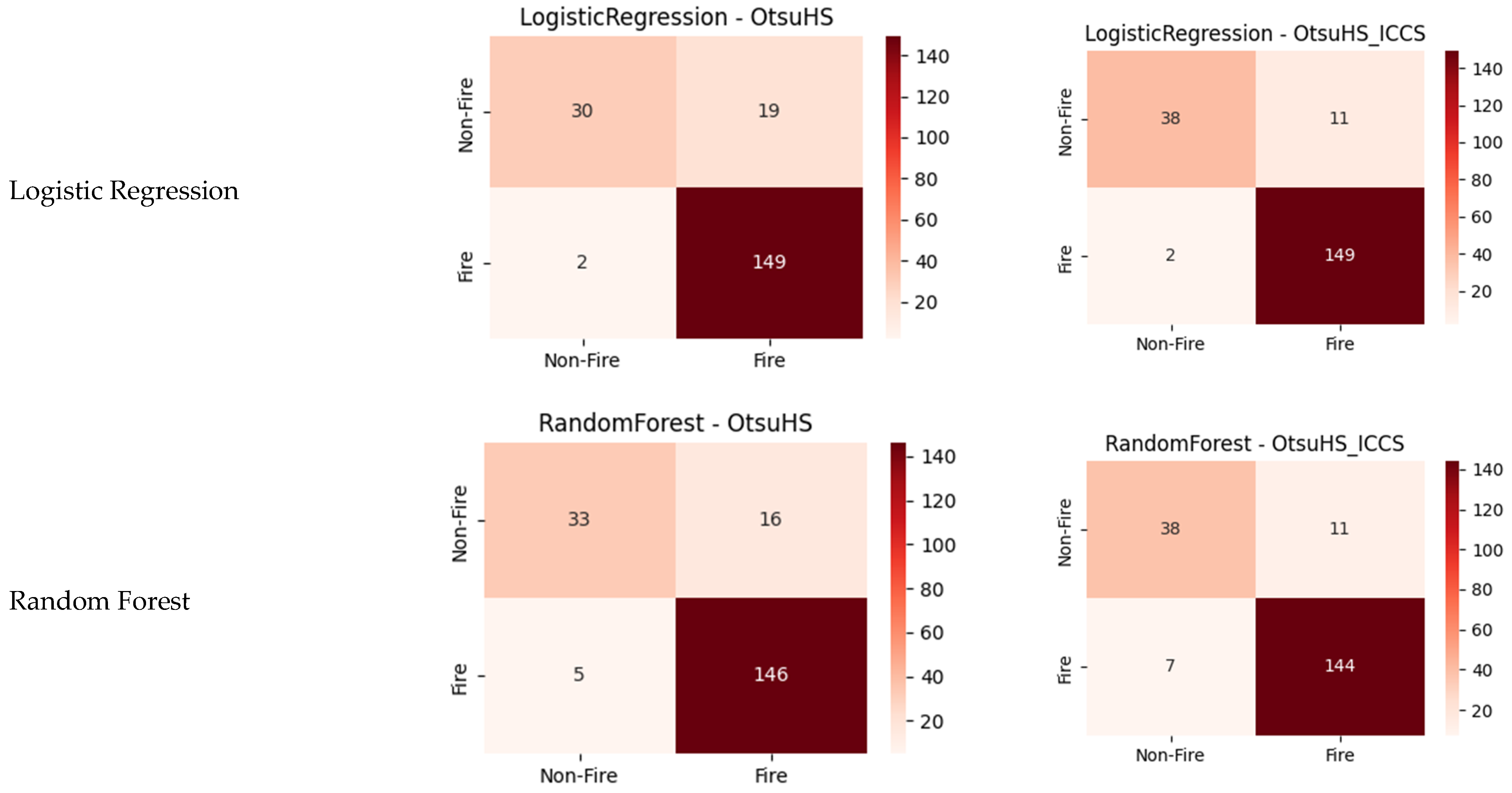
Figure 5 and Figure 6 display the confusion matrices for the test subset and for both datasets.

Table 7. The classification performance of Random Forest, Logistic Regression, and Linear SVM across the (X&Y) dataset derived from the Mendeley dataset. Evaluation metrics were computed for fire and non-fire classes. Accuracy is the average value.

Model	Precision Fire	Recall Fire	F1 Fire	Precision Non-Fire	Recall Non-Fire	F1 Non-Fire	Accuracy
Random Forest (Otsu + HS)	0.872	0.773	0.820	0.741	0.851	0.792	0.807
Random Forest (Otsu + HS + ICCS)	0.880	0.785	0.830	0.753	0.859	0.803	0.817
Logistic Regression (Otsu + HS)	0.867	0.797	0.831	0.759	0.839	0.797	0.815
Logistic Regression (Otsu + HS + ICCS)	0.870	0.800	0.833	0.762	0.843	0.801	0.817
Linear SVM (Otsu + HS)	0.884	0.866	0.875	0.828	0.851	0.839	0.860
Linear SVM (Otsu + HS + ICCS)	0.881	0.881	0.881	0.843	0.843	0.843	0.862

and

Table 8. The classification performance of Random Forest, Logistic Regression, and Linear SVM across the (X&Y) dataset derived from the Kaggle dataset. Evaluation metrics were computed for fire and non-fire classes. Accuracy is the average value.

Model	Precision Fire	Recall Fire	F1 Fire	Precision Non-Fire	Recall Non-Fire	F1 Non-Fire	Accuracy
Random Forest (Otsu + HS)	0.893	0.993	0.941	0.969	0.633	0.765	0.905
Random Forest (Otsu + HS + ICCS)	0.925	0.987	0.955	0.949	0.755	0.841	0.930
Logistic Regression (Otsu + HS)	0.887	0.987	0.934	0.938	0.612	0.742	0.895
Logistic Regression (Otsu + HS + ICCS)	0.931	0.987	0.958	0.950	0.776	0.853	0.935
Linear SVM (Otsu + HS)	0.901	0.967	0.933	0.868	0.673	0.758	0.895
Linear SVM (Otsu + HS + ICCS)	0.927	0.951	0.939	0.832	0.776	0.803	0.910

show the average performance metrics. To ensure the reliability of the classification performance comparison, five experimental runs were conducted. As illustrated in Table 7 and Table 8, the model’s classification performance on both datasets is at its lowest when no local ICCS features are included. However, combining color information with spatial dynamics significantly improves the classification performance. Table 7 summarizes the classification performance for the Mendeley dataset. The performance of the Linear SVM model with ICCS-embedded features was higher than that of competitive machine learning models. Logistic Regression and Random Forest showed slightly lower performance, maintaining precision and recall close to those of the Linear SVM model for both fire and non-fire classes. These models demonstrate the ability to reduce false alarms without compromising sensitivity to real fire events. Table 8 summarizes the classification performance for the Kaggle dataset. As in the previous case, the inclusion of ICCS features significantly enhances performance across all models. The highest performance is achieved by Logistic Regression with the ICCS, followed closely by Random Forest. Because the Kaggle dataset includes non-fire images of undamaged trees, the recall for the fire class was slightly lower, and the recall for the non-fire class was higher. This may indicate some difficulty in distinguishing between positive and negative samples, leading to a lower false positive rate, i.e., low recall but high precision, for the fire class. Overall, these results highlight the effectiveness of ICCS features in improving classification accuracy and robustness in more uniform datasets.

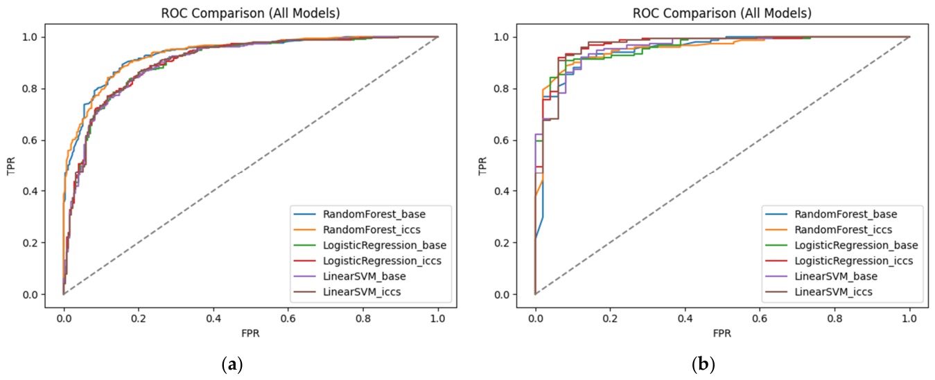
We further examined performance based on receiver operating characteristic (ROC) analyses. Figure 7 presents the ROC curves for all evaluated models. Figure 7a highlights that features provided by the Mendeley dataset are slightly less effective than those from the Kaggle dataset. Data provided by Kaggle consistently achieved areas under the ROC curve close to 1.0 across all classifiers and features, indicating strong discriminative ability (Figure 7b). These findings further support the value of ICCS embedding features and the potential of local chromatic instability to improve classification performance.

Table 9. McNemar statistical validation was conducted on baseline classifiers using two representations for each classifier: global color (X) and ICCS-enhanced features (Y). The models were trained on the same training data (X or Y) and tested on the same test set (X or Y). n00 is the number of samples correctly classified by the classifier for the X and Y datasets; n01 is the number of samples correctly classified for X and misclassified for Y; n10 is the number of samples correctly classified for Y and misclassified for X; n11 is the number of samples misclassified by the classifier for the X and Y datasets.

Dataset	Classifier	n00	n01	n10	n11	Statistic	p-Value
Mendeley dataset	Random Forest	496	12	12	70	0.041667	0.838256
	Logistic Regression	479	0	1	110	0	1
	Linear SVM	474	1	2	113	0	1
Kaggle dataset	Logistic Regression	178	2	9	11	3.272727	0.07044
	Linear SVM	176	4	9	11	1.230769	0.267257
	Random Forest	171	8	10	11	0.055556	0.813664

shows the McNemar statistical test results. This comparison examines the performance of a classifier across two scenarios: testing using the global color descriptor (X dataset) and testing using ICCS-enhanced feature representations (Y dataset). McNemar’s test measures the effect of classification mistakes of the same classifiers on paired data by determining whether there is a statistically significant difference between the proportions of errors made by the model.

For both datasets, even if the classifiers might not have produced identical predictions, there were no statistically significant prediction discrepancies (p > 0.05). The classifiers performed similarly on both test sets (X and Y), with a comparable error rate. Essentially, the classifier’s behavior remained unchanged. The Logistic regression classifier, for the Kaggle dataset, was closer to the cutoff, but there was still no statistically significant difference in performance when it was trained and tested on the X and Y feature datasets (p = 0.07044).

To validate our work, we used three well-known deep learning models as additional comparison tools to assess the performance of our proposed feature sets X and Y. We conducted a comparative analysis using Swin Transformer, MobileViT, and ViT-Base-16 models. The deep learning models were not retrained, fine-tuned, or heavily optimized to improve their results.

Table 10. The classification performance of deep learning models across the Mendeley dataset.

Model	Precision Fire	Recall Fire	F1 Fire	Precision Non-Fire	Recall Non-Fire	F1 Non-Fire	Accuracy
Swin Transformer (Otsu + HS)	0.927	0.982	0.954	0.974	0.898	0.935	0.940
Swin Transformer (Otsu + HS + ICCS)	0.94	0.985	0.962	0.979	0.918	0.947	0.960
MobileViT (Otsu + HS)	0.917	0.925	0.921	0.901	0.890	0.895	0.897
MobileViT (Otsu + HS + ICCS)	0.960	0.854	0.904	0.832	0.953	0.888	0.910
ViT-Base-16 (Otsu + HS)	0.889	0.907	0.898	0.875	0.851	0.863	0.830
ViT-Base-16 (Otsu + HS + ICCS)	0.893	0.818	0.854	0.784	0.871	0.825	0.848

and

Table 11. The classification performance of deep learning models across the Kaggle dataset.

Model	Precision Fire	Recall Fire	F1 Fire	Precision Non-Fire	Recall Non-Fire	F1 Non-Fire	Accuracy
Swin Transformer (Otsu + HS)	0.910	0.900	0.900	0.910	0.694	0.788	0.860
Swin Transformer (Otsu + HS + ICCS)	0.986	0.907	0.945	0.854	0.959	0.903	0.920
MobileViT (Otsu + HS)	0.968	0.801	0.877	0.60	0.918	0.726	0.830
MobileViT (Otsu + HS + ICCS)	0.983	0.748	0.850	0.553	0.959	0.701	0.880
ViT-Base-16 (Otsu + HS)	0.901	0.967	0.933	0.868	0.673	0.759	0.895
ViT-Base-16 (Otsu + HS + ICCS)	0.929	0.954	0.941	0.844	0.776	0.809	0.910

present the classification performance.

The classification performance of complex deep learning models is almost identical to that of the problem at hand.

For machine learning classifiers, the computation time for the Kaggle dataset ranged from 10 to 30 min, while the Mendeley dataset took 30 to 60 min. Logistic Regression was the fastest classifier, and the Linear SVM using ICCS features was the most computationally expensive. Meanwhile, deep learning algorithms needed more processing time. The Kaggle execution times varied from 25 to 70 min, depending on the feature representation. The Mendeley times ranged from 80 to 240 min. MobileViT was the least computationally expensive, at around 70 min. ViT-Base-16 with the ICCS was the most expensive, at 240 min. Swin Transformer had intermediate execution times ranging from 40 to 180 min.

4. Discussion

The forest fire images in our library included pictures of forest fires and regions that had not been burnt. The experimental results demonstrate that the proposed framework achieved significant improvements in the accuracy of fire/non-fire detection. The ICCS embedding features aimed to simultaneously guarantee high accuracy, recall, and precision for fire-image classification. The performance of the models with ICCS-embedded features was superior to that of their global color variable model counterparts.

In our first experiment, we used the HSIC and three kernels to evaluate the statistical dependence between various random variables in nonlinear dependence measures. The overall results indicated significant differences among X = [Otsu_R, Otsu_G, Otsu_B, HS_R, HS_G, HS_B] and Y = [Otsu_R, Otsu_G, Otsu_B, HS_R, HS_G, HS_B, ICCS_R, ICCS_G, ICCS_B] features. The results for the HSIC and nHSIC suggest that the ICCS captures local chromatic instability patterns that are not represented by conventional global color descriptors. This finding supports integrating the ICCS with Otsu and histogram statistics, as the combined feature set can capture both global color distributions and local fire dynamics.

In a second experiment, we used the Silhouette index to assess the separability among X and Y feature sets. When using global color features (X), both fire and non-fire samples in the feature space are difficult to distinguish (Figure 4). Addressing ICCS features (Y) improves class separation (Figure 3). For the Kaggle dataset, the Silhouette index increased from 0.26 to 0.57, while for the Mendeley dataset, it rose from 0.27 to 0.42. Models based on global color characteristics struggle to handle complex situations involving uncertainty about whether samples are fire or non-fire (or like flames). The ICCS reflects the subtle yet noticeable local variations observed in fire images, while the global characteristics simply illustrate the extensive color dispersion in the images.

The classification results indicate the same trend. The results from models trained solely on global features were typically less reliable, particularly for the more challenging Mendeley dataset. Following the incorporation of ICCS features, the overall classification performance improved across all evaluated metrics. The analysis of class-wise performance metrics reveals a trade-off between sensitivity and specificity across different classifiers. This trade-off signifies that improvements in true positive values often result in a decline in false positive values and vice versa. The proposed approach demonstrates high recall for fire class, particularly for the Kaggle dataset, indicating a strong ability to identify solutions for image-based fire detection systems. In practical fire mitigation, recall is more important than precision because any omission in fire detection could lead to a serious disaster. Occasionally, precision and recall values drop below 0.8 for the non-fire class, but this is not critical. For practical fire prevention, this suggests that reducing false negatives over false positives should be prioritized. The improvements in F1-score and recall, important for detecting genuine fire events, demonstrate the proposed approach’s suitability for maintaining high fire detection performance across various datasets. We used McNemar’s test to assess the disagreement between classifiers’ predictions when using the X and Y feature sets during training and testing. For both datasets, there were no statistically significant discrepancies in classifier predictions.

The experimental findings indicate that dataset quality is important. Fire data is typically collated based on the owner’s interests, such as fire locations, perimeters, or severity. This raises concerns about data inhomogeneity that could affect its use. Thus, the Kaggle dataset has more consistent image settings, resulting in a balanced distribution across fire, smoke, and normal categories. The Mendeley dataset is more challenging to use due to its variable lighting and background characteristics. Given the heterogeneity of the datasets considered in this study, we strengthen our analysis by providing a baseline comparison using machine learning models. This finding aligns with Zaman et al. [26]’s results. They stress the importance of choosing classifiers and preprocessing methods that suit the dataset’s characteristics. Different models are particularly effective for specific dataset features, especially in forest fire detection.

Finally, our goal was to show that our lightweight feature extraction approach was more practical in terms of computational cost. The proposed ICCS-based approach is computationally efficient, interpretable, and suitable for real-time applications, while maintaining competitive performance relative to substantially more complex deep learning solutions. In this framework, the lightweight feature extraction approach exhibits a combination of (i) low-dimensional feature representation, (ii) the absence of deep-network training and backpropagation, (iii) operation on standard CPU hardware without GPU requirements, and (iv) reduced computational time compared with transformer-based architectures. Deep learning models require significant computational resources, longer execution times, and more complex implementations. The proposed ICCS-based approach, as a lightweight and computationally efficient alternative, is well-suited for resource-constrained environments and real-time fire monitoring applications.

Classical classifiers such as Logistic Regression, Random Forest, and Linear SVM were quicker than deep learning systems. Machine learning methods analyzed the Kaggle dataset in 10 to 30 min, while the Mendeley dataset took 30 to 180 min, depending on the classifier and ICCS features. Logistic Regression was the fastest traditional classifier, whereas Linear SVM using ICCS features was the most computationally costly. In the meantime, deep learning algorithms required more time to process. The execution times on Kaggle were 25–70 min, while those on Mendeley were 80–240 min. MobileViT was the least computationally costly deep learning method, whereas ViT-Base-16 with the ICCS was the most expensive. Swin Transformer was intermediate, ranging from 40 to 180 min depending on feature representation. This comparison is purely for cross-checking the proposed approach’s utility and is not intended for refining deep learning models. Our approach offers a key advantage: it is faster than deep learning alternatives, while still providing comparable (if occasionally slightly lower) performance.

Direct comparisons with published state-of-the-art methods remain challenging because of differences in datasets and evaluation protocols. However, to situate the proposed ICCS framework within the existing fire-detection literature,

Table 12. Comparison with representative fire-detection studies. N/A indicates not available data.

Study	Method	Dataset	Recall	F1-Score	Accuracy
Liping et al. [5]	Gradient Features + SVM	Proprietary flame dataset	Reported as high detection performance	N/A	N/A
Liang et al. [6]	RF feature selection + BPNN	Video fire dataset	N/A	N/A	Improved over baseline methods
Joutsalainen et al. [14]	MobileNetV3 (Fireframe)	Wildfire smoke dataset	0.984	N/A	mAP50 = 1.00
Lv et al. [15]	CCi-YOLOv8n	Web-Fire, D-Fire	High recall in complex scenes	N/A	Reported improvement over YOLOv8n
Proposed method	Linear SVM + ICCS	Mendeley	0.881	0.881	0.862
Proposed method	Logistic Regression + ICCS	Kaggle	0.987	0.958	0.935

compares the best-performing ICCS-based model with representative studies reported in recent years. The results presented here should be interpreted as an indirect benchmark rather than a strict head-to-head evaluation. Nevertheless, the proposed ICCS descriptors achieve recall values up to 0.987 and F1-scores up to 0.958 on publicly available datasets, demonstrating that lightweight chromatic-instability features can provide performance comparable to considerably more complex learning architectures while incurring substantially lower computational cost. The literature demonstrates a clear trend toward increasingly complex deep learning architectures, including CNN-, YOLO-, and Transformer-based frameworks. These methods often achieve excellent detection performance but generally require substantially larger computational resources, extensive training data, and longer inference times. In contrast, the proposed ICCS representation is designed as a lightweight feature extraction method that can be integrated with conventional machine learning classifiers while maintaining competitive classification performance.

The provided comparison highlights a critical real-time application. While the global feature (X dataset) excels at detecting the fire class only for the Kaggle dataset, local chromatic instability features (Y dataset) offer the most robust detection capability for both fire and no-fire classes. This makes them the most viable candidates for creating automated systems that can rapidly and precisely detect fires in pictures. The approach is also ideal for real-time applications because it is both user-friendly and computationally efficient. It is computationally efficient because it employs lightweight feature extraction techniques (global color statistics and ICCS) with traditional machine learning models. Traditional machine learning models performed competitively within the proposed framework, thereby validating its robustness.

5. Conclusions

This study introduced a reliable, feature-driven fire detection system that combines global color descriptions with local chromatic instability indicators. Within the framework of the suggested technique, the Spatial Chromatic Instability Index (ICCS) measures local fluctuations in RGB values. The ICCS accurately describes the unpredictability and changeability of fire. The key difference between using global color features, such as histogram dispersion and Otsu segmentation, and ICCS features is that the former reliably fail to identify fire in visually complex images. Separating and classifying the fire and non-fire classes might be made more effective by merging global color features with local chromatic instability indicators.

The comprehensive evaluation across both global color descriptions and local chromatic instability indicators revealed critical insights into feature representation. The experimental results show improved Silhouette coefficients and classification performance metrics. The results consistently showed that the ICCS provides information that is largely independent of the global descriptors and improves class separability and classification performance when combined with them.

In the case of deep learning models, the performance gains come at a substantially higher computational cost, with longer execution times and greater implementation complexity. The proposed ICCS-based approach is not a replacement for state-of-the-art deep learning models. Instead, it is a computationally efficient, lightweight alternative suitable for resource-constrained environments and real-time fire monitoring applications. Due to this, it is appropriate for applications requiring real-time processing and early warning systems. The system demonstrated strong performance in distinguishing fire from non-fire conditions, particularly in minimizing false alarms without sacrificing real fire detection capability.

Nevertheless, this method still has some limitations. While effective for identifying the erratic color behavior of flames, the ICCS approach relies solely on the RGB space for analysis. It does not account for temporal analysis to detect fires. Also, yellow, orange, or red objects can create local chromatic instability similar to fire, leading to false alarms. Similarly, dark or bright scenes reduce the accuracy in differentiating between fire and background. In future work, we will build on this work and expand the investigations to various color spaces or combine color analysis with smoke detection or thermal imaging to improve reliability. Also, more diverse datasets will improve generalization. In addition, exploring vision transformers may further enhance the performance of fire detection systems.