Optimizing Fire Perimeter Geometry in Cellular Automata Wildfire Models Using Ant Colony Optimization

Abstract

Simulating wildfires in large areas is commonly achieved by methods based on cellular automata (CA), especially when the available computational resources are limited. However, the discrete nature of CA, in both the space and time domains, often leads to systematic distortions and artifacts in the generated fire perimeter geometry. This article presents a hybrid wildfire simulation framework that integrates a two-dimensional CA model with an ant colony optimization (ACO) algorithm to improve fire perimeter shape representation. The proposed approach employs ACO to iteratively adjust the coefficients integrated into the local CA transition rules, under varying environmental and forestry fuel conditions. This optimization step corrects geometric inconsistencies arising from the underlying nature of a CA model, while preserving their computational advantages. The hybrid implementation is evaluated through simulation experiments under varying environmental and fuel conditions, demonstrating improved agreement between simulated and reference fire perimeters, compared to a baseline CA model.

1. Introduction

For millions of years, wildfires have served as a natural mechanism to restructure and regenerate landscapes and ecosystems. In recent years, however, an alarming increase in wildfire ignitions, especially near inhabited areas, raises grave concerns about the dangers to human lives [1]. Moreover, their impact on the natural environment is enormous, resulting in millions of tons of emitted CO₂ [2], huge animal losses and the destruction of pristine forests. Critical communication and transportation infrastructure, agricultural lands, pastures and residential buildings are frequently among the most severely affected land uses [3].

To mitigate the life-threatening nature of wildfires, researchers have focused on studying the physical phenomena related to fire spread, in order to unfold their transition mechanics. Following advances in computational methods, numerical simulations of fire spread metrics [4,5,6] have started to be conducted by scientists, to assist firefighting personnel in suppression efforts, aid civil protection authorities to plan evacuation strategies in the vicinity of high-risk areas and inform land management agencies in the design and implementation of prescribed burning plans [7]. The tools most commonly employed by experts include fire danger indices and fire spread models, which vary in their conceptual frameworks, ranging from purely physics-based to purely empirical, depending on the specific application domain and accuracy requirements.

Among them, cellular automata (CA)-based modeling of wildfires is one of the most robust techniques proposed in the literature. They capture complex fire dynamics with simple semi-empirical local transition rules and are easy to implement, while maintaining a lightweight computational footprint. Their computational advantage is derived from their underlying raster-based architecture, which significantly accelerates geometric calculations. This characteristic makes the method viable for deployment even on devices with limited computational and power resources, such as portable devices.

However, their reliance on empirically tuned local transition rules introduces structural and statistical challenges that limit their applicability to general cases of wildfires. In particular, they rely on sub modules (such as estimators of wind impact, fuel moisture content and fuel flammability) involving an extensive set of parameters and coefficients, which require user tuning. Moreover, it is extremely difficult for a non-expert user—whether in forest science, wildfire dynamics, or meteorology—to fully comprehend the physical significance and impact of each parameter when conducting a simulation in a real-world case, or to distinguish which variables are correlated together. Parameterization and calibration are the Achilles’ heel of these models, making them prone to overfitting, yielding apparently accurate reconstructions of specific fire events, while providing limited predictive performance outside their calibration domain. In addition, because the effects of the individual parameters are aggregated into a single ignition probability, distinct parameter sets may produce similar macroscopic fire patterns, which may lead to ambiguous model interpretations by non-expert users.

One particular limitation of CA-based wildfire methods is their difficulty in reproducing accurate wildfire perimeters [8,9,10]. This limitation primarily arises from the bounded spatial resolution of the simulation grid and the inherently discrete nature of the modeling framework. In most CA models, it is assumed that all properties within a single simulation cell are spatially homogeneous. For example, fuel characteristics or meteorological conditions within a cell are represented by a single aggregated variable, regardless of their variability inside that cell. Furthermore, the use of discrete cell states typically restricts each cell to binary conditions (e.g., completely burned or unburned), thereby excluding intermediate states, such as partial combustion, re-ignition, or changes in burn status caused by evolving wind direction or fuel moisture. These simplifications can lead to geometric artifacts in the simulated fire perimeter, particularly in regions of high curvature, and are especially evident when coarse spatial resolutions are employed.

This behavior is not unknown to researchers and a wide range of improvements and optimization strategies have been proposed to address it. These approaches span multiple levels of model complexity, ranging from parameter optimization and fine-tuning of existing CA formulations [11,12], to structural enhancements that map physical processes (e.g., wind, slope, and fuel properties) into probabilistic transition rules [13] and modified cell shapes [14]. More extensive modifications include the introduction of variable simulation time steps [8,15,16,17], continuous or multi-valued cell states [17,18], and vector-based propagation schemes [16], all of which aim to reduce discretization artifacts and improve the realism of simulated fire perimeters. These advances in two-dimensional cellular automata for wildfire simulation are comprehensively reviewed in [19], where many techniques addressing these limitations are discussed.

Ant colony optimization (ACO) [20] is a robust metaheuristic optimization technique that has been successfully applied to a wide range of problems across numerous scientific and engineering disciplines [21,22]. Although ACO is primarily known for its effectiveness in discrete combinatorial optimization problems, several variants have been developed to address continuous optimization tasks. ACO implementations for continuous solution spaces extend the original framework by adapting the originally discrete, single-dimension pheromone representation to a continuous form. In addition, they introduce new solution construction mechanisms, thereby enabling their application to Continuous Optimization Problems (COPs). Among them, Socha and Dorigo proposed the ACO_R [23] algorithm, which is considered the most widely applicable, while maintaining the original formulation of the ACO framework. Previously proposed variants do exist, like the one proposed by Bilchev and Parmee [24] (CACO algorithm), the API algorithm by Monmarché et al. [25] and the hybrid implementation of the CIAC algorithm by Dréo and Siarry [26]. Later approaches include Liu et al.’s [27] ACO based on a position distribution model, DACO_R [28] and ARACO [29].

In this paper, we formulate a COP aimed at the calibration of a two-dimensional CA wildfire simulator under parameter uncertainty. The COP’s objective is to identify an optimal set of CA model parameters and coefficients, which will minimize the discrepancy between the burn perimeter produced by the CA simulation and that generated by a simplified theoretical fire spread model based on the elliptical model [30,31,32]. Uncertainty in the model parameters is explicitly addressed by formulating the calibration task over continuous, high-dimensional search spaces. This process is inherently computationally demanding, due to the size and complexity of the parameter space, which renders exhaustive or gradient-based search strategies impractical. Consequently, the use of metaheuristic optimization methods capable of efficiently handling continuous variables becomes essential, as they provide a viable means to explore the search space and identify near-optimal solutions, within reasonable computational budgets.

To satisfy near-real-time simulation requirements, external inputs such as meteorological conditions and fuel composition mapping are expected to reach the core simulation module at irregular intervals, via streamed data sources or, potentially, through crowdsourced in-field observations. The proposed calibration scheme is designed to support the incremental assimilation of dynamically acquired data, enabling continuous parameter updates during runtime. This progressive integration enhances both the accuracy of the simulation and the reliability of real-time fire spread estimation.

The remainder of this paper is organized as follows. Section 2.1 presents the outline of a typical CA wildfire simulation model, Section 2.2 describes an extension of the same CA model coupled with weather data, while Section 2.3 modifies the model even further by introducing a dynamic neighborhood configuration. Section 2.4 describes a methodology of estimating a wildfire’s perimeter via the simple ellipse model, while Section 2.5 provides the framework of an ACO algorithm for COPs. In Section 2.6, we estimate the computational complexity of the proposed tuning mechanism while Section 2.7 examines the study area located in Glyfada, Greece, and the environmental conditions during the reference event. Section 3 presents the results obtained from the application of the ACO_R-based parameter tuning method. Finally, Section 4 provides a discussion of the methodology and the key observations arising from its application, while Section 5 concludes the paper.

2. Materials and Methods

2.1. A Two-Dimensional CA-Based Wildfire Simulator

Before evaluating the proposed tuning mechanism, it is necessary to formally define the CA-based wildfire spread simulator employed in this study. We build upon a two-dimensional CA wildfire spread formulation introduced by Alexandridis [33], which has been extensively described and extended by him and other researchers [34,35]; it has also been evaluated in real-world fire events. This framework is particularly suitable for our purposes due to its comprehensive representation of the main drivers of fire spread, including fuel characteristics, terrain properties, and meteorological conditions. Although the original framework also incorporates the suppressing effects of firefighting tactics, this component is excluded in the present work, since accurate and reliable data on aerial firefighting operations are difficult to obtain, and their inclusion would mislead the interpretation of potential simulation and fine-tuning findings. In addition, the modeling of spotting behavior is also omitted, as it relies on probabilistic formulations with more tunable parameters—many of which are difficult to estimate without access to in-field observations—that could obscure our benchmarking and hinder a clear assessment of the proposed tuning scheme.

In a typical CA-based simulator, the landscape is represented as a two-dimensional grid composed of a finite set of cells, each corresponding to a spatial unit of terrain. The spatial resolution of the grid is defined as $l_{cell}\times l_{cell}$ where $l_{cell}$ is the cell side. A crucial assumption is that each cell represents a homogeneous area in terms of fuel properties, topography, and environmental conditions. Accordingly, each cell in the grid is associated with a discrete state, describing its current fire-related condition. During grid initialization, we rely on external data sources like the Corine Land Cover (CLC) or specific fuel maps, if available, to assign the corresponding starting states. In the context of this work, state definitions include only four states: no fuel, unburned, burning, and burned. More detailed formulations may introduce additional intermediate states to account for varying combustion phases, such as ignition and active flaming, or implement states with continuous ranges. The state of a cell at a given time step is determined by its previous state and by the states of neighboring cells, reflecting the localized nature of wildfire propagation. The number of neighboring cells defines the neighborhood structure, with the Moore neighborhood (eight adjacent cells) being the most common.

The temporal evolution of the fire is captured in fixed, discrete simulation steps of duration $dt$ and is governed by a set of transition rules that are applied synchronously to all cells at each step. Transition rules are typically probabilistic formulas that incorporate environmental and physical factors including but not limited to fuel type, fuel moisture content, wind speed and direction and slope. The fine-tuning of the transition probabilities based on the above parameters allows the CA model to approximate complex fire behavior, while maintaining computational efficiency.

The transition rules used by the model [33] are defined as follows:

• A cell containing no fuel cannot change state.
• A burned cell cannot change state.
• A burning cell transitions to the burned state at the next time step.
• An unburned cell may transition to the burning state at the next time step with probability $P_{burn}$ if at least one cell in its neighborhood is in the burning state.

Transition rules 2 and 3 reveal that the model prevents any cell from reigniting. While reignition does occur in real-world conditions, the model assumes that all fuel within a cell is fully consumed during the duration of a single simulation time step. Consequently, the simulation time step cannot be fixed to a specific duration, as doing so would violate the temporal characteristics of real fire behavior. While dynamic time step implementations have been proposed in the literature [15,16], we retain the original formulation to preserve model simplicity and enable consistent benchmarking of our fine-tuning mechanism.

The calculation of the $P_{burn}$ probability (Equation (1)) is conducted as follows:

$$P_{burn} = P_0(1+P_{veg})(1+P_{den})P_w{P}_s,$$

(1)

where $P_0$ denotes a base probability due to an adjacent burning cell, assuming zero wind and no elevation difference. We must note that $P_0$ is not a direct physical analogue of ignition probability, but a model parameter whose effective use requires knowledge of additional fire behavior-induced factors, fine-tuning, and is inherently subject to uncertainty. Alexandridis [34] states that $P_0$ can be computed as a function of the user-specified length of the cell side $l_{cell}$, the Rate of Spread (ROS) and the duration of the simulation time step. $P_{veg}$ and $P_{den}$ are coefficients related to the density and type of fuel within a modeled cell. These parameters are commonly derived from lookup tables that map predefined fuel classes to corresponding $P_{veg}$ and $P_{den}$ values [33,34], typically constructed using information obtained from remote sensing-based fuel characterization techniques.

The term $P_w$ is related to the impact of the wind speed and direction on the propagation of the fire (Equation (2)) while $P_s$ models the influence of terrain slope (Equation (3)) on fire spread, accounting for the enhanced preheating of unburned fuels caused by flame tilt when fire propagates upslope. In general, wind influences both the direction and the rate of fire spread, while terrain slope contributes to additional acceleration and can markedly affect fire behavior and propagation patterns. These terms are calculated as follows:

$$P_w= e^{\left[V\right(c_1+c_2(\cos \left(\theta \right)-1)\left)\right]},$$

(2)

$$P_s=e^{a_s{\theta }_s} ,\hspace{1em} {\theta }_s={tan}^{-1}\left({\displaystyle \frac{E_1-E_2}{d(E_1,E_2)}}\right),$$

(3)

where $c_1,c_2$ are tunable parameters that model the impact of wind speed and direction to the ignition probability, $V$ is the wind speed (m/s) and $\theta$ is the angle formed between the wind direction and the examined direction of local fire spread (°). Term $a_s$ is another user-tunable parameter linking the terrain influence, $E_1$, $E_2$ is the elevation of the cells under examination (m) and $d(E_1,E_2)$ is the Euclidian distance of cells $E_1$, $E_2$ (m). Equation (3) models the effect of slope (derived from the difference in elevation of the centroids of the cells) on fire spread, capturing the well-documented behavior that fire propagates more rapidly when moving upslope and slows down when moving downslope. This occurs because, on an upslope, flames are tilted closer to the unburned fuel, enhancing heat transfer through radiation and convection and promoting faster preheating and ignition [36].

2.2. A Weather-Coupled CA Model

An extension of the typical CA model presented in Section 2.1, incorporating the impact of the fuel moisture content (FMC) on fire spread, has been proposed in [34]. Equation (1) for the $P_{burn}$ probability is modified to incorporate an additional term, $P_m$, accounting for the effect of the FMC in the ROS (Equation (4)).

$$P_{burn}=P_0(1+P_{veg})(1+P_{den})P_w{P}_s{P}_m,$$

(4)

The term $P_m$ can be expressed as a function of the FMC (Equation (5)), where $\alpha ,b$ are user-specified parameters [34,37]. This function is derived by non-linear interpolation obtained from sample fires and models the negative exponential relationship between the ROS and FMC.

$$P_m=\alpha e^{-b·FMC},$$

(5)

The FMC is rarely measured directly in practice, as it requires considerable time and a large number of sampling points across the study area, which is unrealistic during a wildfire event. Direct measurements are typically conducted only to validate FMC model estimates in real-world scenarios. In the context of wildfire simulation, the FMC is usually obtained indirectly from weather and environmental data. In our implementation, we compute the equilibrium moisture content (EMC), a widely used and practical technique for estimating fuel moisture. In Equation (6), we adopt the EMC formulation presented by Simard in [38] used in NFDRS [39], which uses $H$ (relative humidity in %) and $T$ (temperature in °F) as input variables. Alternatively, the EMC can be obtained using the Nelson model [40]; however, this approach is not adopted, as it introduces additional tunable parameters that may complicate the interpretation of the results of tuning the CA parameters. Nevertheless, both methods do not account for rainfall, which is known to influence the fuel moisture content [41]. Due to limited availability of precipitation data, this factor could not be incorporated into our study.

$$EMC=\left\{\begin{array}{l}0.03229+0.281073·H-0.000578·T·H H<10\%\\ 2.22749+0.160107\cdot H-0.014784\cdot T 10\%\le H<50\%\\ 21.0606+0.005565·H^2-0.0003505·H·T-0.483199·H H\ge 50\%\end{array}\right.,$$

(6)

According to the equilibrium moisture time-lag theory [42,43], fuels dry following a negative exponential curve under constant temperature and relative humidity conditions. Therefore, the FMC should, in principle, be updated accordingly for each fuel class. However, to avoid this complication, we decided to use weather data upscaled to 5 min intervals (Section 2.7). Given that the original data have a temporal resolution of one hour, this refinement is not expected to introduce significant additional uncertainty compared to the inherent noise in the input data [44]. Consequently, it is omitted in our implementation.

2.3. A Dynamic Neighborhood CA Model

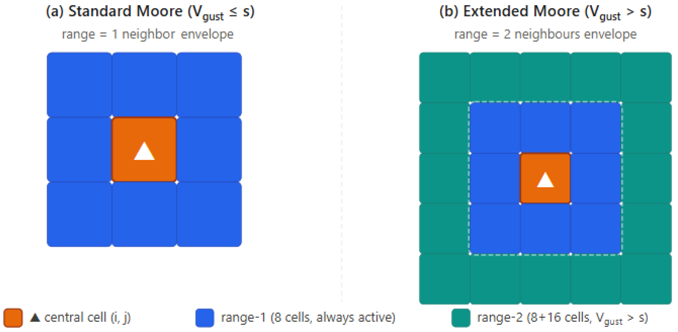
We can also extend the CA model presented in Section 2.1 by introducing dynamic neighborhood size configuration, inspired by Freire [35]. While a typical Moore neighborhood configuration adequately captures local spread dynamics under moderate wind conditions, it fails to represent the long-range spotting and accelerated propagation observed empirically when wind gusts exceed critical thresholds. To address this limitation, we introduce a dynamic neighborhood switching mechanism controlled by a wind gust threshold parameter $s$ (in km/h).

At each simulation time step, the wind gust speed $V_{gust}\left(\mathrm{t}\right)$ is read from the available meteorological data. When $V_{gust}\left(\mathrm{t}\right)\le \mathrm{s}$, the standard Moore neighborhood is retained, comprising 8 neighboring cells at distances of $l_{cell}$ and ${\sqrt{2}l}_{cell}$ from the central cell. When $V_{gust}\left(\mathrm{t}\right)> s$, the neighborhood is expanded to an extended Moore configuration, consisting of a 5 × 5 window of 24 surrounding cells (Figure 1). In any case, the slope coefficient $P_s$ (Equation (3)) is computed using the Euclidean distance and the corresponding elevation differences.

The parameter $s$ can be treated as a calibration variable within the ACO_R optimization framework alongside the remaining tuning parameters, allowing its value to be inferred from the expected fire perimeter data (using the technique described in Section 2.4) rather than assumed a priori.

2.4. Estimating the Perimeter of a Wildfire Based on the Simple Ellipse Model

At a macroscopic level, extracting the perimeter of a wildfire in a pre-fire event is effectively equivalent to simulating its spatial spread. In this context, the predicted fire perimeter is represented by the geometric evolution of the fire front at specific time points. Comprehensive two- or three-dimensional fire behavior models simulate additional physical properties of the fire, such as the ROS, fireline intensity, flame length, and fire-induced interactions with the atmosphere. Perimeter estimation can be regarded as a simplified, yet computationally efficient means of assessing the potential spatial extent of wildfire impact, rather than a full characterization of fire behavior or damage severity.

Perimeter estimation is most commonly approached through methods based on Huygens’ wavelet principle, whereby each point along an existing fire front is treated as the origin of a secondary wavelet, and the envelope of these wavelets defines the subsequent fire perimeter [45]. While the vector-based application of Huygens’ principle effectively represents the curvature of the fire perimeter, the Minimum Travel Time (MTT) algorithm [46] offers a computationally efficient alternative by modeling fire spread as a network optimization problem over a spatial grid. The MTT discretizes the solution space into a grid of nodes (similar to CA) and calculates the fastest travel path (employing a cost function that examines fuel, terrain, etc.) from the ignition to source. This method preserves the physical analogy of Huygens’ principle, while maintaining a reasonable computational footprint, making it ideal for large-scale estimations.

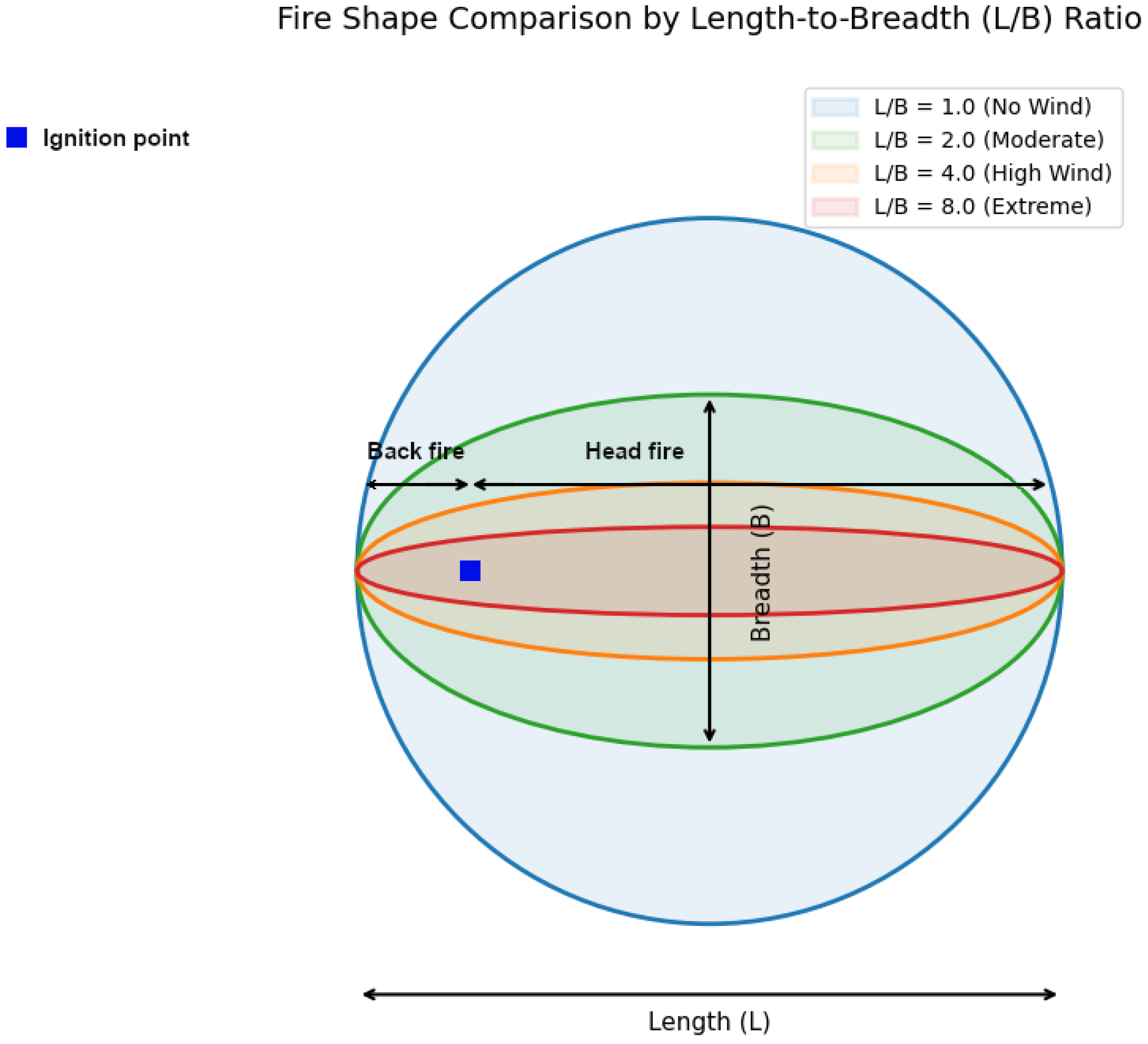
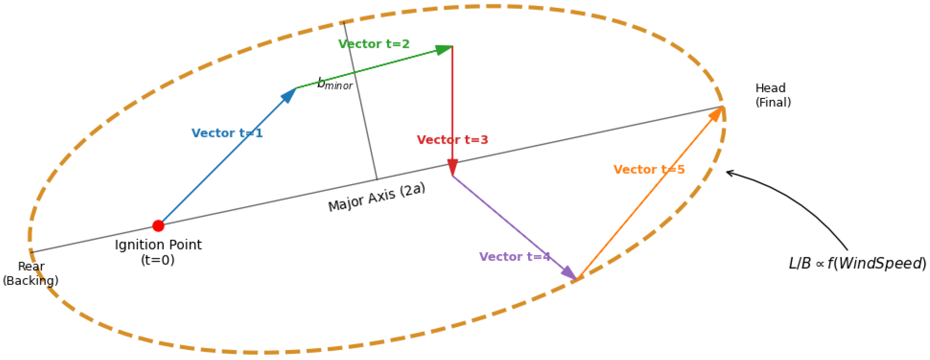
In this paper, we employ a simplified approach based purely on the elliptical growth model [30]. This efficiency is critical because the model serves as the objective function for the ACO_R algorithm; therefore, it requires extremely fast evaluation times. In the proposed approach, fire propagation is represented by generating spread vectors at discrete time intervals. Rather than tracking a complex perimeter, the aggregate expansion is encapsulated within a single bounding ellipse. The geometry of this ellipse is governed by the length to breadth (L/B) ratio, which is expressed as a function of wind speed and direction [31,47], as illustrated in Figure 2.

The proposed method approximates fire growth by constructing a single elliptical envelope around a piecewise vector path. The process begins by calculating a sequence of spread vectors at discrete time steps (at a lower frequency than in the CA), where the magnitude and direction of each segment are determined by the weather conditions and fuel combustibility (e.g., using Rothermel’s fire spread model), creating a ‘zig-zag’ trajectory of the theoretically expected spread. Instead of retaining an arbitrary polygon from this complex polyline, the method derives a simplified enclosing ellipse that is mathematically fitted to this vector chain. The geometry of this envelope is defined by a major axis extending from the final vector coordinate (the fire head), backward through the ignition point to a calculated rear boundary, ensuring the ignition source remains collinear with the primary axis of propagation. This construction forces the ignition point to lie along the major axis in the rear focus point, while the shape’s eccentricity is controlled by the L/B ratio derived from empirical models like those presented in [31,47,48]. As an example, Figure 3 depicts a simulated elliptical perimeter, derived from the aggregation of five consecutive spread vectors.

Although the formulation for estimating the length to breadth ratio (L/B) proposed by Simard [49] accounts for the influence of the standard deviation of wind direction, its application requires detailed and accurate in-field wind observations. In the absence of such data, this approach would introduce an additional source of uncertainty. Therefore, in our implementation, the L/B ratio is derived using Alexander’s expression [47] (Equation (7)). An alternative would have been to adopt Anderson’s [31] formulation; however, its reliance on a double ellipse representation would substantially increase model complexity and was thus not pursued.

$${\displaystyle \frac{L}{B}}=1.0+0.00120·W^{2.154}$$

(7)

In this formula, $W$ is the 10 m open wind speed in km/h and it is applicable for wind speeds up to 50 km/h.

The outline of the method is given in Algorithm 1 below:

Algorithm 1. Theoretical Ellipse Envelope Construction
1.	Input: weather vector weather, ignition point ignition
2.	point ← ignition
3.	vectors ← {point}
4.	for each sampling interval i do
5.	find dominant vegetation and calculate ROS during time i
6.	vi ← ROS * dt with direction from point towards weather[i].direction
7.	point ← vi
8.	vectors ← { vectors ∪ vi }
9.	end for
10.	LB ← CalculateLB(weather.speed, vectors)
11.	envelope ← CalculateEllipse(ignition,vectors,LB)
12.	return envelope, area(envelope)

2.5. An ACO Algorithm for Continuous Optimization Applied to CA Parameter Calibration

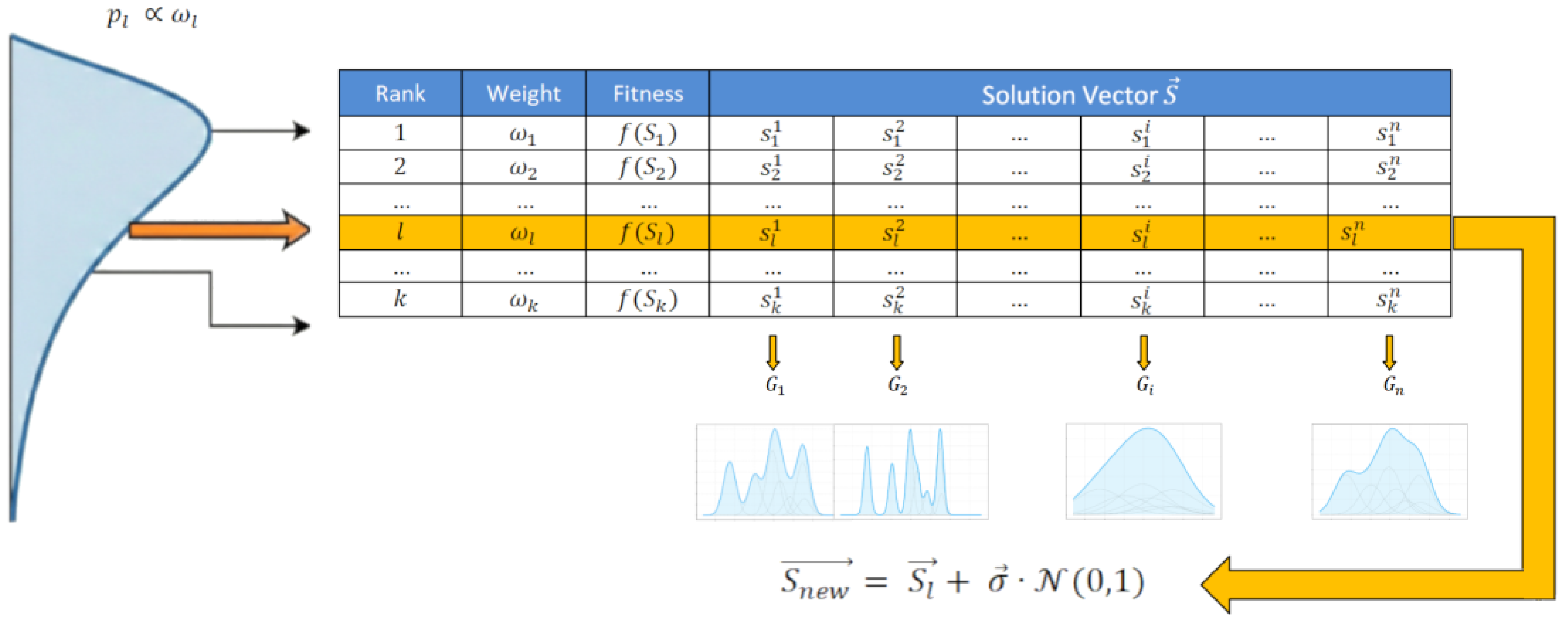
In the context of this paper, we employ the ACO_R [23] algorithm, since it is a clear metaphor for the original ACO framework [20]. The main novelty lies in replacing the incremental probabilistic construction of solutions used in ACO with a solution archive. Specifically, the ACO_R framework maintains a finite archive $T$ containing $k$ solutions, ranked according to their objective function values. Each solution in the archive is associated with a weight $w_i$ that reflects its quality (according to the objective function) and determines its influence on the sampling process. New candidate solutions are generated by each artificial ant in $n$ (dimension of solution space) incremental steps by (indirectly) sampling a set of Gaussian kernel $G_i$ Probability Density Functions (PDFs), where each solution stored in $T$ serves as the mean of a Gaussian kernel (Equation (8)):

$$T =\{S_1,S_2,\dots ,S_k\}$$

(8)

The objective function $f:S\to \mathbb{R}$ is being optimized (usually minimized) where $S\subseteq {\mathbb{R}}^n$ is the search space and $n$ is the problem’s dimensionality. A candidate solution $S=\{x_1,x_2,\dots ,x_n\}$ must also be feasible and therefore must not violate the constraints of the problem, denoted by the constraint set $\Omega$.

The construction of solution archive $T$ is illustrated in Figure 4. The $k$ best-so-far known solutions are stored according to their fitness, and the weight factor for the ith solution ${\omega }_i$ is calculated as follows (Equation (9)).

$${\omega }_i={\displaystyle \frac{1}{qk\sqrt{2\pi }}}{e}^{(-{\displaystyle \frac{{(i-1)}^2}{{2q}^2{k}^2}})},$$

(9)

where $i$ is the rank of the solution in $T$, and $q$ is a user-specified parameter (analogous to the exploitation–exploration parameters in discrete ACO) that influences the behavior of the artificial ants. When $q$ is selected close to zero, the algorithm heavily biases the search towards the best-ranked solution. Conversely, higher values of $q$ promote a wider exploration of the search space, typically at the cost of a significantly slower convergence speed. An artificial ant selects the $S_l$ solution from archive $K$ with probability $p_l$ as follows (Equation (10)):

$$p_l = {\displaystyle \frac{{\omega }_l}{{\sum }_{r=1}^k{\omega }_r}},$$

(10)

Then, it constructs a new candidate solution $S_{new}$ by sampling a Gaussian PDF around the “neighborhood” of the selected solution: $S_{new}^i= S_l^i+ {\sigma }_l^i·\mathcal{N}\left(\mathrm{0,1}\right)$ (where $l$ is the selected solution from $T$ and $i$ the ith dimension of the problem). Each standard deviation is calculated as follows (Equation (11)):

$${\sigma }_l^i = \xi {\displaystyle \sum _{e=1}^k}{\displaystyle \frac{|s_e^i-s_l^i|}{k-1}},$$

(11)

where $\xi >0$ is a user-specified parameter that regulates the balance between exploration and exploitation, analogous to the pheromone evaporation rate in a discrete ACO framework. Higher values of $\xi$ increase the distance between newly generated solutions and the best-known ones, enhancing exploration at the expense of convergence speed.

Finally, the effect of the pheromone update is accomplished by examining the newly generated solutions and, if they exhibit better fitness than those stored in $K$, inserting them with the simultaneous removal of the worst-performing solutions, to keep the archive size constant.

To apply the ACO_R algorithm for fine-tuning the CA model parameters presented in Section 2.1, we formulate the problem as the following constrained optimization problem:

$\mathrm{m}\mathrm{i}\mathrm{n}\mathrm{i}\mathrm{m}\mathrm{i}\mathrm{z}\mathrm{e}$	$f\left(X\right)=|Estimate{d}_{Area\left(X\right)}-Simulate{d}_{Area\left(X\right)}|$
$X$	$X=\{P_0,c_1,c_2,{\alpha }_s\}$
$subject to$	$0\le P_o\le 1$
	$0\le c_1\le 1$
	$0\le c_2\le 1$
	$0\le {\alpha }_s\le 1$

Due to the absence of well-established physical constraints in the literature for the parameters within a CA framework, the slope and wind influence coefficients were treated as dimensionless sensitivity factors. Consequently, in our tuning experiments, they were set to vary within the bounded range [0, 0.5] to explore the model’s response under both enhancing and inhibiting conditions. For the CA variants described in Section 2.2 and Section 2.3, the same formulation applies, with the vector $X$ becoming $X=\{P_0,c_1,c_2,{\alpha }_s,a,b,s\}$; the parameter bounds employed by each of these CA variants are presented in Section 3.

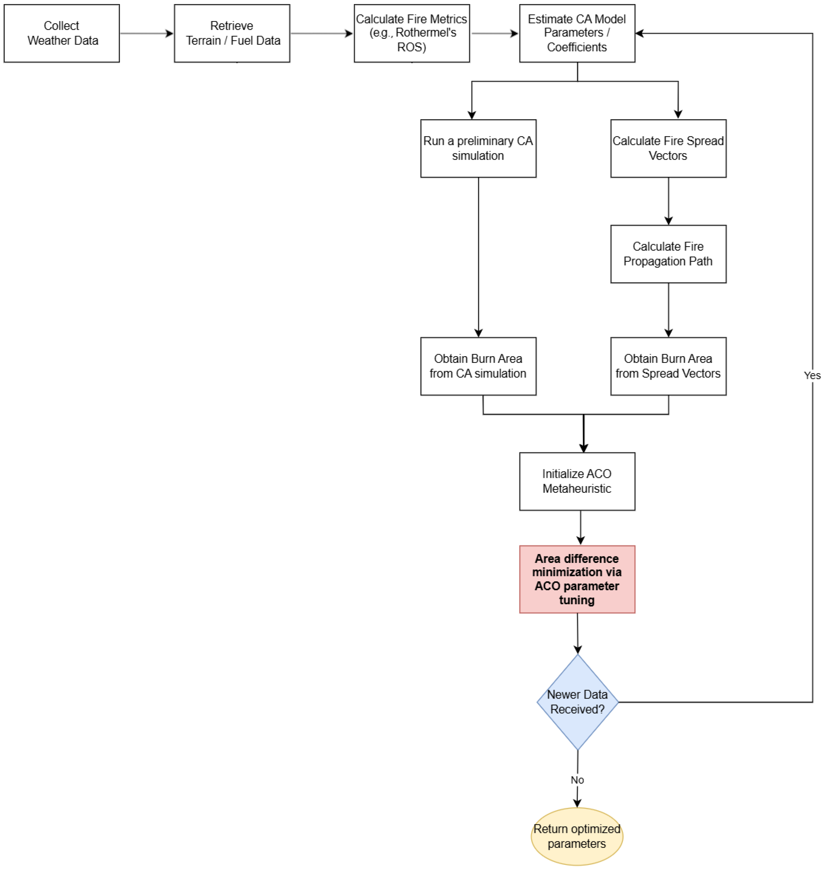
The parameter calibration process employing the ACO_R metaheuristic is presented in the pseudocode that follows (Algorithm 2), while the flowchart of the method (focused on the case where streamed data from crowdsourcing inputs are received from in-field users, in order to improve the wildfire spread simulation) is given in Figure 5. Firstly, a preliminary CA simulation (for a limited duration of time) is conducted with default values $X=\{P_0,c_1,c_2,{\alpha }_s\}$ for the parameters that will be optimized. For the same duration, a theoretical elliptical envelope of the same fire is constructed according to Algorithm 1 (using fewer sampling points). The objective function is formulated as the area difference between the area of the CA simulation and the area of the envelope. Then, after i iterations of the ACO_R metaheuristic, new values for $X$ are obtained that can be used to re-run the CA simulation for a greater duration.

This parameter calibration process is repeated whenever new crowdsourced data become available from in-field users or when the CA simulation yields poor performance. The evaluation of the objective function (during each iteration of ACO_R) with updated $X$ values unavoidably leads to a new execution of a CA simulation. Consequently, these preliminary simulations are conducted over a shorter duration than the full simulation with the optimized values.

Algorithm 2. CA parameter tuning by the ACOR metaheuristic
1.	Input: weather vector weather, ignition point ignition, time duration
2.	set initial values for parameters $\mathit{X}=\{P_0,c_1,c_2,{\alpha }_s\}$
3.	simulated_grid ← runCA_Simulation(weather,ignition,X,duration)
4.	simulated_area ← area(simulated_grid.burned_cells)
5.	while new data are available
6.	envelope ← Algorithm 1(weather,ignition)
7.	objectiveFunction() ← |area(envelope)-area(simulated_area)|
8.	T,ω ← intializeSolutionArchive(InitialRandomSolution,q)
9.	for each iteration i do
10.	for each ant k do
11.	select solution l from T with probability pl according to ωl
12.	sk ← xl
13.	σk ← calculate_σ(ξ,l)
14.	${\mathit{s}}_{\mathit{k}}^{\mathit{new}} \leftarrow {\mathit{s}}_{\mathit{k}}+{\mathit{\sigma }}_{\mathit{k}}·\mathcal{N}\left(\mathbf{0,1}\right)$
15.	end for
16.	update T with new ant solutions according to objectiveFunction()
17.	end for
18.	${\mathit{X}}_{\mathit{new}} \leftarrow$T[0]//best solution in T
19.	end while
20.	simulated_grid ← runCA_Simulation(weather,ignition,Xnew,durationnew)

2.6. Estimation of the Tuning Scheme’s Complexity

To estimate the method’s computational complexity, it is necessary to identify the key components of the tuning process: the ACO_R layer executed for I_ACOR iterations, and the subsequent evaluation of the objective function, which involves a CA simulation over I_CA iterations, for each of the candidate solutions generated by ACO_R. Note that I_CA refers to the iterations required for the CA simulation during the tuning process (preliminary run), not the full duration of the simulated event for which the CA is eventually executed.

The ACO_R layer complexity is derived from the mechanism artificial ants use to explore the search space, and how the solution archive is maintained at each iteration. For each I_ACOR iteration, $m$ artificial ants generate an equal number of candidate solutions through sampling $n$ Gaussian kernels (number of decision variables). Then, the solution archive of size $k$ must be merged with the $m$ newly generated solutions. The size of archive $T$ remains $k$; therefore, the $m$ worst solutions will be evicted from $T$ for the next iteration of ACO_R. Hence, the complexity of the optimization process by ACO_R is $C_{ACOR}= O\left(I_{ACOR}·(m·n+(m+k)log (m+k\left)\right)\right)$, where the left side of the complexity corresponds to the generation of the candidate solutions and the right side with reforming $T$ in order to contain the $k$ most promising solutions out of the k existing and m candidate solutions; since the k existing solutions are already sorted, faster implementations are possible, but, as we will see, other costs dominate. Specifically, to identify the fitness of the m candidate solutions, we need to evaluate the objective function for them, by running a preliminary CA simulation.

The complexity of the CA simulations is not directly related to the grid size, but to the number of cells transitioning from burning state to burned. In a CA run, we do not process every cell at every step; instead, we only examine the neighbors of currently burning cells. Therefore, the complexity of CA is $C_{CA}= O(I_{CA}·B_{avg}·N·{Estimate}_{Pburn})$ where $B_{avg}$ is the average number of burning cells per step and $N$ the neighborhood configuration (e.g., for a Moore neighborhood, N = 8). ${Estimate}_{Pburn}$ also introduces computational overhead, since cell burn probabilities must be updated at each iteration (only for neighboring cells) due to changing conditions (e.g., wind direction). Nevertheless, accessing these environmental conditions from external sources may introduce additional I/O overheads that are beyond the scope of this analysis.

The computational complexity of the proposed tuning mechanism is thus dominated by the objective function evaluations. While the ACO_R framework introduces an overhead, the primary cost is the iterative execution of the CA simulator for each candidate solution. In the worst (unrealistic) case, where the fire covers the entire grid, the complexity is $C_{total}=O(I_{ACOR}·m·G·{Estimate}_{Pburn})$, where $G$ is the number of cells in the grid, but then, the simulation exits before all $I_{CA}$ iterations have completed.

Hence, we can express the complexity of the method solely via the complexity of the CA as follows (Equation (12)):

$$C_{total}\approx O[I_{ACOR}·(m·C_{CA}\left)\right]$$

(12)

2.7. Study Area

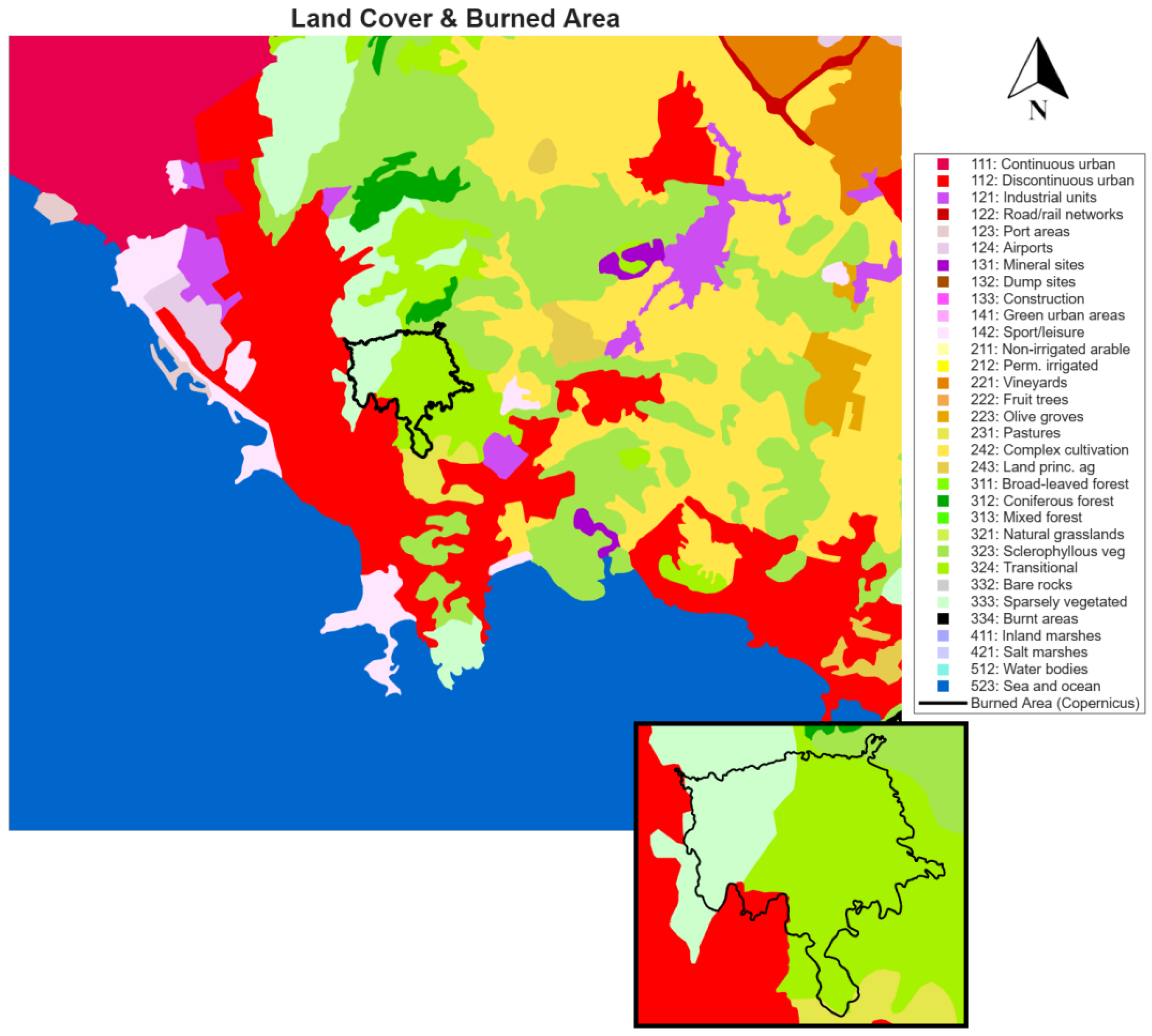
To evaluate the improvement in the predicted burned area achieved by the CA wildfire simulator, we selected a wildfire that occurred on Mount Hymettus near the suburb of Glyfada, Greece (Figure 6). The event took place on 4 June 2022, at 12:50 pm local time. Although the affected area was relatively small (about 432 ha according to the EMSR576 Copernicus Activation Report), the fire spread rapidly, and the incident was considered highly serious due to its proximity to residential areas.

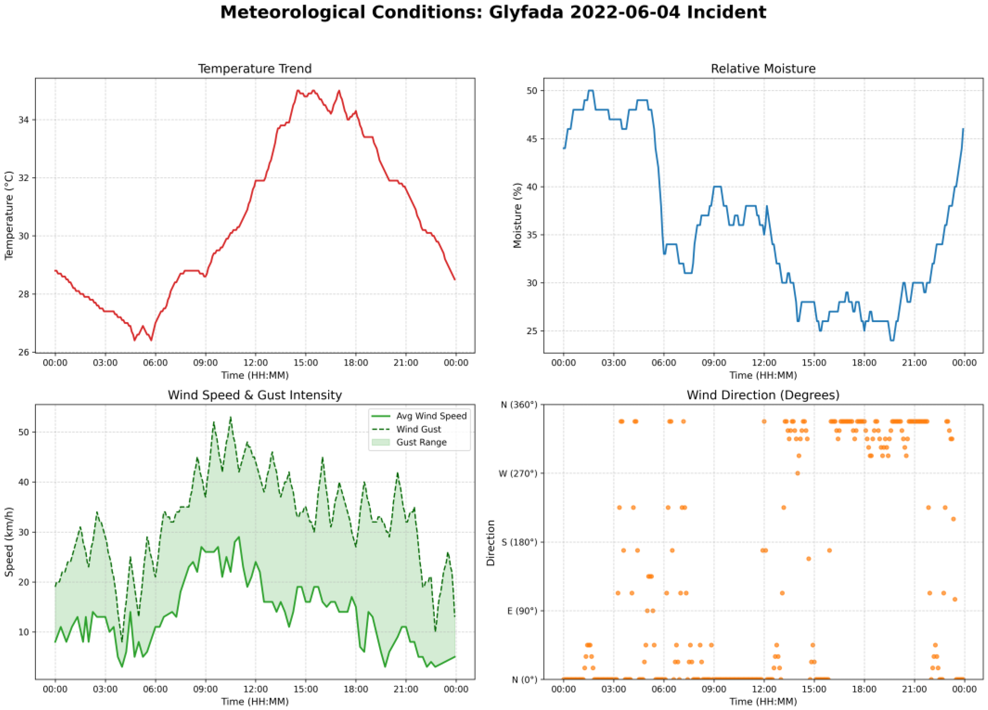
Meteorological conditions were obtained from a nearby weather station, which was part of the network of automatic stations of the National Observatory of Athens (Figure 7). To ensure high temporal granularity for the simulated reconstruction of the incident, the datasets were processed at a 5 min resolution. It should be noted that while the visualization presents continuous 5 min data points, these values were derived via linear interpolation from the original, lower-frequency sampling rate of the weather station. This upsampling method provides a smoother trend analysis, though the primary peaks and troughs remain anchored to the original observation points. Special caution should be exercised when interpreting wind direction trends. Because the data were upsampled from a lower-frequency source, the directional values between the original observations are subject to interpolation bias. Consequently, large-scale shifts in wind direction are captured effectively, whereas high-frequency directional fluctuations should be interpreted as indicative rather than as absolute.

For each CLC class in the study area, we map it to the P_den and P_veg coefficients employed by the CA model, based on experimental analysis and similar test cases reported in the literature [33,34].

Table 1. CLC land cover classes identified near the study area and their corresponding P_den and P_veg coefficients used in the CA wildfire simulation.

CLC Code	Type	Pden	Pveg
111	Continuous urban fabric	−1.0	−1.0
112	Discontinuous urban fabric	−0.7	−0.8
121	Industrial or commercial units	−0.7	−0.8
123	Port areas	−1.0	−1.0
124	Airports	−1.0	−1.0
131	Mineral extraction sites	−0.9	−0.9
142	Sport and leisure facilities	−0.5	−0.5
223	Olive groves	0.6	0.45
231	Pastures	0.45	0.4
242	Complex cultivation patterns	0.5	0.5
243	Land principally occupied by agriculture, with significant areas of natural vegetation	0.55	0.5
312	Coniferous forest	0.75	0.7
323	Sclerophyllous vegetation	0.65	0.6
324	Transitional woodland/shrub	0.35	0.4
333	Sparsely vegetated areas	0.0	−0.15
523	Sea and the ocean	−1.0	−1.0

presents the CLC classes identified in the study area along with their corresponding coefficient values.

3. Results

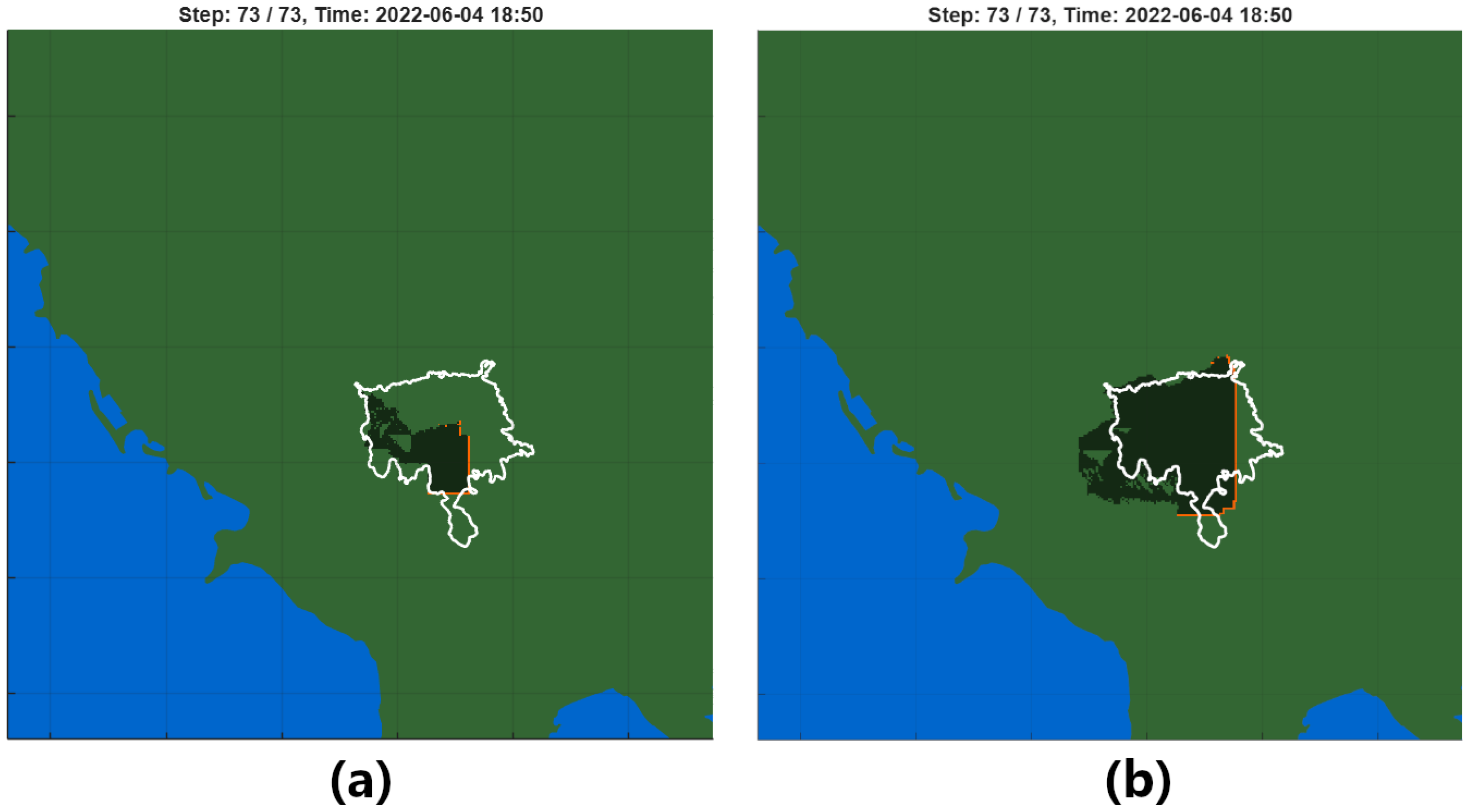
To evaluate the efficacy of the proposed parameter tuning mechanism, an initial wildfire spread simulation was conducted over a 6 h horizon using the typical CA-based simulator of Section 2.1, configured with the parameters listed in

Table 2. Parameters used in the initial CA simulation.

Parameter	Value	Parameter	Value
$P_0$	0.450 *	$a_s$	0.078
$c_1$	0.045	$l_{cell}$	30.6 m
$c_2$	0.131	$dt$	5 min

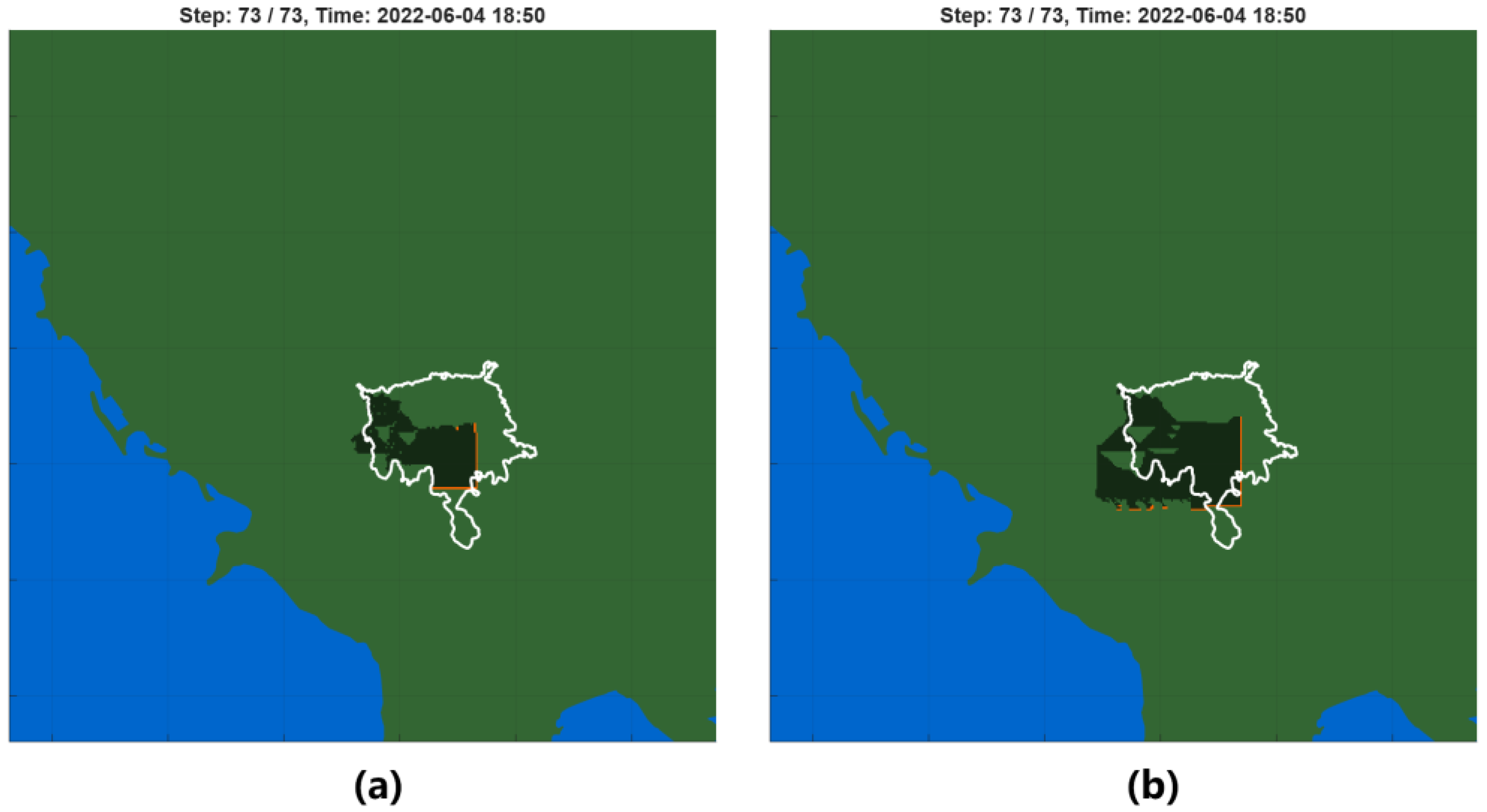
* $P_0$ value selected based on the literature [33,34] and proportional to the calculated no-wind, no-slope ROS of about 2.4 m/s, based on calculations conducted in the Behave Plus 6 software [50].

. This simulation yielded a simulated burned area of 149.3 ha, which underestimates the observed burned area by −65.45% (see Figure 8a); this will serve as a baseline for the final simulation, along with the estimated burned area reported by the EMSR576 report.

The final simulation output was obtained through a multi-stage calibration procedure that was conducted in the following stages:

• Preliminary Simulation and Envelope Construction: A truncated 150 min (2.5 h) preliminary CA simulation was executed using the same parameters as in the baseline simulation. For the same duration, a theoretical elliptical envelope was constructed following the methodology in Section 2.4. This involved generating spread vectors and fitting an encapsulating ellipse, where the semi-major axis was aligned with the vector extending from the ignition point to the final spread frontier. The calculated envelope was projected onto grid cells to enable a direct comparison between methods.
• Objective Function Definition: The objective function for minimization was defined as the absolute difference in the number of burned cells (of the same size) between the preliminary CA simulation output and the theoretical elliptical model output. It should be noted that each objective function evaluation requires both the CA method and the elliptical envelope model to be executed, using the parameters determined during the optimization stage.
• ACO_R Metaheuristic Optimization Stage: The Ant Colony Optimization for Continuous Domains (ACO_R) algorithm was deployed using the configuration parameters specified in

  Table 3. Parameters used for the ACO_R algorithm.

  Parameter	Value	Parameter	Value
  Number of ants	5	$q$	0.05
  Solution archive size	30	$\xi$	0.10
  Number of iterations	35 *

  * Due to the small number of decision variables to be tuned, the extended size of solution archive T and the narrow bounds identified, experimentation showed that ACO_R required only a limited number of iterations to converge to the optimum.

  . During each objective function evaluation, ACO_R initiated a new CA simulation instance, iteratively adjusting the input parameters based on the candidate solutions generated.
• Convergence and Validation: After 35 iterations, the ACO_R metaheuristic converged on an optimal parameter set listed in

  Table 4. Optimal parameter set for the CA model obtained through ACO_R optimization.

  Parameter	Value	Parameter	Value
  $P_0$	0.085240	$a_s$	0.036826
  $c_1$	0.352091	burned cells in 6 h	5753 burned cells
  $c_2$	0.248356

  , which yielded a fitness value of 11 cells for the optimization function. These optimized parameters were subsequently applied to the final 6 h CA simulation. The calibrated run resulted in a burned area of 538.5 ha, representing a significant adjustment from the initial (non-optimized) simulation and demonstrating improved alignment with the observed wildfire burned area (see Figure 8b).

The number of ants primarily controls the sampling density of the search space, where larger values improve exploration and solution robustness but increase computational cost, while smaller values reduce computational effort at the risk of insufficient search coverage. Based on the sensitivity analysis, five artificial ants (Table 3) were selected as a compromise between sufficient exploration of the solution space since the number of decision variables in the baseline case is relatively small. Similarly, the archive size affects solution diversity and stability. In contrast, the parameters $q$ and $\xi$ significantly influence convergence behavior. Lower $q$ values accelerate convergence speed but may lead to premature convergence, whereas higher values improve exploration. Likewise, smaller $\xi$ values promote local exploitation, while larger values enhance global search at the expense of convergence speed. The selected parameter values provide a balanced trade-off between exploration and exploitation, taking into account that the decision variables are bounded within relatively small intervals, which reduces the need for extensive global exploration.

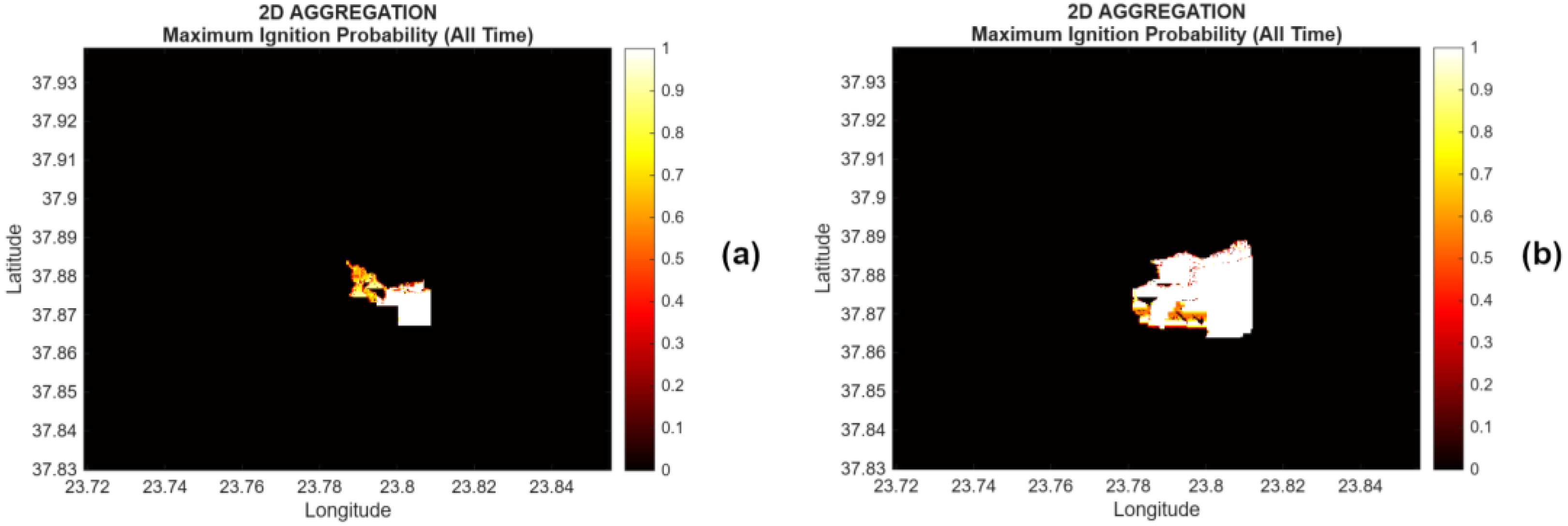
Figure 9 shows an aggregate probability map of the simulated grid area before (a) and after (b) parameter tuning, at the same simulation time steps. The effect on cell ignition probabilities is indicated by the color scale in the legend. To eliminate the temporal dimension imposed by the discrete time-stepping of the CA method, the ignition probabilities ($P_{burn}$) were aggregated over the entire simulation horizon and projected onto a square spatial grid. Each cell value therefore represents the cumulative likelihood that the corresponding cell will ignite during the simulation. This time-integrated probability field provides a spatially explicit representation of fire susceptibility, allowing direct comparison of the overall spread tendency and intensity patterns between methods. The resulting maps reveal differences in spatial propagation, highlighting areas of increased or reduced ignition propensity that are not immediately apparent from the stepwise temporal evolution alone. At each time step, the CA does not evaluate ignition across the entire grid; instead, only cells in the neighborhood of already ignited cells are considered candidates for ignition. This reflects the local propagation mechanism of the model, where fire spread is governed by neighborhood interactions rather than global evaluation of all grid cells.

Subsequently, the same procedure was applied to tune the CA variant incorporating weather coupling (Section 2.2), which introduces two additional decision variables, $a$ and $b$, representing the fuel moisture content.

Table 5. Parameters used in the initial CA variant with weather coupling simulation.

Parameter	Value	Parameter	Value
$P_0$	0.450	$a$	2.015
$c_1$	0.045	$b$	0.091
$c_2$	0.131	$l_{cell}$	30.6 m
$a_s$	0.078	$dt$	5 min

presents the parameter values used in the initial (non-optimized) simulation, serving as a baseline for comparison with the optimized results.

Due to the increase in the number of decision variables relative to the previous application, the ACO_R algorithm was appropriately reconfigured to accommodate the expanded search space.

Table 6. Parameters used for the ACO_R algorithm to fine-tune the weather-coupled CA model.

Parameter	Value	Parameter	Value
Number of ants	10	$q$	0.05
Solution archive size	40	$\xi$	0.20
Number of iterations	50

presents the specific configuration used for the ACO_R algorithm. Moreover, given that the term $P_m$ is derived from a non-linear regression analysis conducted by Fernandes [37], the decision variable $a$ was constrained to the range $[2, 3.5]$ and variable $b$ was constrained to the range $[0.05, 0.15]$.

The optimal parameter assignment after the optimization runs using the ACO_R metaheuristic are listed in

Table 7. Optimal parameter set for the CA weather-coupled model obtained through ACO_R optimization.

Parameter	Value	Parameter	Value
$P_0$	0.5159	$a$	3.3634
$c_1$	0.2200	$b$	0.1462
$c_2$	0.3500
$a_s$	0.6170	burned cells in 6 h	3727 burned cells

, while Figure 10 depicts the burned area as simulated by the CA model with weather coupling (a) before optimization and (b) after ACO_R optimization.

Lastly, we performed the same systematic fine-tuning using the ACO_R for the third CA variant introduced in Section 2.3. This formulation incorporates an equivalent number of decision variables to those of the weather-coupled model, with the addition of the parameter $s$, which defines the critical threshold governing the transition from the standard neighborhood configuration to the extended Moore neighborhood scheme. Specifically, when the wind-governing conditions exceed this threshold, the model adaptively expands its interaction domain to non-adjacent cells and subsequently fire spread is accelerated. In

Table 8. Parameters used in the initial CA variant with dynamic neighborhood configuration.

Parameter	Value	Parameter	Value
$P_0$	0.450	$b$	0.091
$c_1$	0.045	s	50 km/h
$c_2$	0.131	$l_{cell}$	30.6 m
$a_s$	0.078	$dt$	5 min
$a$	2.015

, we present the set of parameters employed in the initial CA simulation, prior to the application of any fine-tuning procedures, which are identical to those used in the previous CA variant.

For the optimization of this variant, we adopted the same ACO_R configuration as employed in the previous experiments, ensuring methodological consistency and comparability across these similar models. The bounds for the decision variable $s$ (wind gust in km/h) were defined within the interval [20, 70], based on widely accepted empirical assumptions regarding the behavior of wind-driven wildfires. This range was selected to capture plausible transition thresholds while maintaining sufficient flexibility for the optimization process to explore the parameter space effectively. The optimal assignment of values to the decision variables, as obtained through ACO_R, is presented in

Table 9. Optimal parameter set for the CA variant with dynamic neighborhood configuration obtained through ACO_R optimization.

Parameter	Value	Parameter	Value
$P_0$	0.3907	$b$	0.1412
$c_1$	0.0367	s	36.6141 km/h
$c_2$	0.2285	$l_{cell}$	30.6 m
$a_s$	0.6231	$dt$	5 min
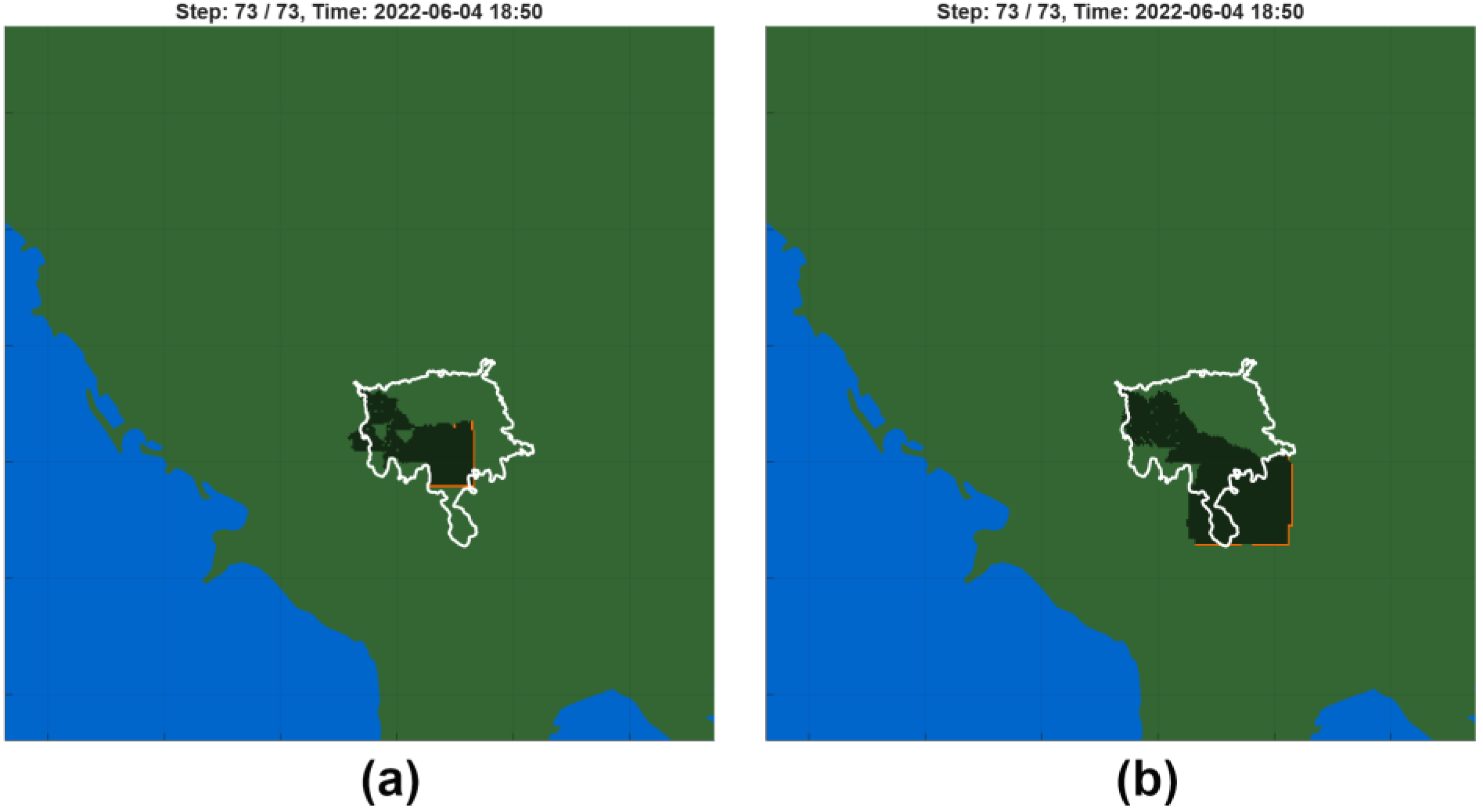
$a$	2.5758	burned cells in 6 h	4275 burned cells

. Furthermore, two comparative simulation runs (a) conducted without fine-tuning, and (b), incorporating ACO_R fine-tuning, are illustrated in Figure 11, thereby highlighting the impact of the optimization procedure on model performance.

Table 10. Comparison of burned areas for each examined test scenario.

Experiment	Burned Area	% of Reported Burned Area	Overlap with Reported Area (%)
EMSR576 report estimation * (Figure 6)	432.2 ha	100%	100%
6 h baseline initial CA simulation (Figure 8a)	149.3 ha	−65.45%	32.78%
6 h CA simulation after ACOR optimization (Figure 8b)	538.5 ha	+24.59%	80.72%
6 h initial CA with weather coupling (Figure 10a)	182.6 ha	−57.75%	38.24%
6 h CA with weather coupling after ACOR optimization (Figure 10b)	348.9 ha	−19.27%	50.58%
6 h initial CA with dynamic neighborhood (Figure 11a)	182.6 ha	−57.75%	38.24%
6 h CA with dynamic neighborhood after ACOR optimization (Figure 11b)	400.2 ha	−7.40%	46.53%

* The actual duration of the wildfire could not be verified. The original burned area can be further adjusted to 447 ha by closing holes in the polygons resulting from remote sensing estimation. Percentage calculations applied to the officially reported burned area.

presents a summary of the experimental results (before and after the fine-tuning procedure), along with their deviation from the reported burned area in terms of the size of the areas and the overlap between the actual and simulated areas.

All algorithms implemented in this study were developed using the MATLAB 2023a software on a typical personal computer. Weather data were stored in JSON files to facilitate easy access and integration with the simulation models. For elevation data, we utilized SRTM (Shuttle Radar Topography Mission) datasets, which provide digital elevation information. Land cover information was obtained from the Corine Land Cover (CLC) database and used in raster format to represent spatial variations in vegetation and land use. This combination of datasets allowed for a comprehensive representation of environmental conditions in the simulation models.

4. Discussion

In this paper, we propose a novel methodology for fine-tuning cellular automata (CA) models for wildfire spread simulation based on the ACO_R metaheuristic. Several points are worth highlighting for the reader.

Firstly, the objective of our work was not to achieve a perfect reconstruction of the presented test case, as the absolute environmental and operational conditions of the real event are difficult to obtain, with many conditions not recorded at all (e.g., mid-flame wind speed, aerial drop locations).

Secondly, the optimization stage was performed using only a few tunable parameters. Although the ACO_R framework is capable of handling hundreds of decision variables, we deliberately adopted a simplified CA formulation [33] to maintain model interpretability and reduce computational complexity.

Thirdly, the probability parameter $P_0$ was also optimized, in contrast to most related studies, where it is assumed to be a constant, representing the probability that a cell ignites under no-wind and no-slope conditions. As the calibration was performed against an elliptical envelope model that incorporates the ROS obtained from Rothermel’s formulation [36] when calculating the spread vectors, the underlying physical behavior associated with $P_0$ is preserved throughout the optimization process and is implicitly captured through its interaction with the remaining tunable parameters.

Fourthly, the probability coefficients $(P_0, a_s,c_1,c_2,a,b,s)$ are treated by the ACO_R algorithm in an agnostic manner with respect to their physical properties and underlying meaning. During the optimization process, the algorithm handles all probability parameters as dimensionless variables to be adjusted, so as to optimize the objective function. Ignition probabilities are calculated as the product of multiple contributing factors (e.g., wind, slope, and fuel flammability), and regardless of what values are assigned to them, the resulting value remains a dimensionless probability. Consequently, there is no unique or direct mapping between probabilities across different simulation outputs.

Fifthly, the choice of objective function imposes a limitation on the performance of the proposed ACO_R-based parameter tuning scheme. In the current implementation, the objective function evaluates only the difference in area between the expected and simulated burned regions, which is a relatively coarse and dimensionless measure. While this approach provides a simple and computationally efficient baseline, a more rigorous evaluation could be achieved using metrics that capture geometric similarity, such as the Hausdorff distance [51], shape similarity indices [52], or a multi-objective function that simultaneously accounts for both area and spatial correspondence between the predicted and theoretical burned shapes. Such enhancements could improve the sensitivity and robustness of the tuning process and will be examined in future work by us.

Sixthly, ACO_R optimizes the parameters to adapt to the prevailing conditions; however, this adaptation is performed in an agnostic manner, which may affect the behavior of the CA. Despite that, the substantial reduction in $P_0$ from 0.45 to 0.085240 in the baseline case markedly lowers the baseline ignition probability under no-wind and no-slope conditions, which directly contributes to reducing the systematic overestimation of the burned area. At the same time, the increase in $c_1$ and $c_2$ amplifies the model’s sensitivity to wind speed and direction, leading to a more responsive and directional spread pattern that better reflects the dynamics of wind-driven wildfires. However, the third CA variant (dynamic neighborhood configuration) resulted in a significant overestimation of the burned area (Figure 11b) outside the reported boundaries. This variant is particularly sensitive to wind compared to the other CA models, making it more prone to amplifying wind-driven spread. The discrepancy likely arises because the model overestimates fire propagation due to wind and/or spotting effects, which typically occur over much shorter time intervals often as brief, intermittent bursts. Interpreting the optimization results in light of the underlying CA transition rules not only clarifies the role of each parameter but also enhances the physical plausibility and practical relevance of the calibrated model.

Finally, the efficiency of the optimization process is constrained by the model used to estimate the theoretical wildfire spread. The suitability of a simple elliptical model for representing complex wildfire behavior—particularly in an urban–wildland interface zone with extensive fire suppression activities, as in the present test case—remains uncertain. In this context, the selection of the elliptical model serves primarily as a baseline for assessing the potential of the optimization technique, rather than as an accurate representation of real-world fire dynamics. This choice was motivated by the fact that elliptical spread models form the foundation of most wildfire simulation software and are still commonly regarded as a standard approach for wildfire perimeter estimation [48].

A key aspect of the proposed methodology is its potential generalizability beyond the specific case study of the Glyfada wildfire. Unlike many other CA models in the literature, which rely on fixed parameterizations calibrated to particular experimental conditions, the present approach introduces a dynamic, data-driven calibration framework based on ant colony optimization. This allows the model parameters to be iteratively updated as new observations become available, making the method inherently adaptable to different wildfire scenarios, fuel types, and environmental conditions. In this sense, the framework is not tied to a specific dataset, but instead provides a mechanism for continuous recalibration, thereby enhancing its applicability across diverse settings. The proposed method can be integrated as a component within a crowdsourced wildfire simulation framework [53], where environmental and fire behavior data are dynamically updated in near-real time using in-field observations from firefighters and other stakeholders. In this context, as landscape and environmental conditions evolve, the method can be deployed on mobile devices to continuously recalibrate any CA model implemented within the simulation software, enabling adaptive and progressively improved simulations.

However, the generalizability of the approach is partly constrained by the formulation of the theoretical fire spread envelope used during the optimization process. In the current implementation, the envelope is constructed using the elliptical model, which assumes relatively homogeneous terrain and steady wind conditions. While a progressive, time-updated construction of the envelope has been introduced to mitigate these limitations, the underlying assumptions may still affect performance in highly heterogeneous environments. To assess the robustness of the method under non-ideal conditions, it was deliberately tested in the Glyfada wildfire scenario characterized by heterogeneous vegetation, significant elevation variation, and variable wind conditions. Despite the mismatch between the simplifying assumptions of the envelope model and the actual conditions, the method managed to generate new calibrated parameters under which the different CA variants achieved satisfactory simulation accuracy, indicating that the proposed tuning framework retains practical effectiveness even outside its nominal assumptions. Overall, these results suggest that while the envelope formulation may impose some limitations, the adaptive nature of the optimization scheme enables the method to generalize reasonably well across a range of realistic wildfire scenarios. Further improvements in envelope modeling are expected to enhance its applicability in even more complex environments.

Future work could focus on relaxing the simplifying assumptions of the current elliptical formulation in order to better capture complex fire dynamics. One promising direction is the adoption of wavefront-based approaches inspired by Huygens’ principle [45,54], whereby the fire perimeter is represented as the evolving envelope of multiple local spread sources. Such an approach would allow the generation of more irregular and physically realistic fire shapes, particularly under heterogeneous fuel conditions, complex topography, and variable wind. In addition, future developments should explicitly account for fire suppression activities, such as aerial water drops, which are commonly applied in fires near inhabited areas (such as in the Glyfada area fire) and can significantly alter fire spread patterns. Incorporating these effects would require extending the objective function of the ACO_R to accommodate dynamic, complex geometries and localized reductions in spread probability. These future enhancements are expected to improve both the realism and the general applicability of the proposed framework.

5. Conclusions

We presented and evaluated a novel approach for fine-tuning the parameters of a typical cellular automata (CA)-based wildfire spread model, by employing an optimization framework relying on the Ant Colony Optimization for Continuous Domains (ACO_R) metaheuristic. The proposed method integrates a spread vector tracking mechanism that represents fire propagation through an elliptical approximation, serving as a reference for the objective function. Although the number of decision variables in this study was small, the literature demonstrates that ACO_R can address substantially more complex optimization problems, involving hundreds of decision variables. More advanced CA-based wildfire models typically require calibration of a larger set of parameters, particularly when sufficient and high-quality data are available (e.g., tree height for estimating potential spotting behavior). Future research should investigate the performance and robustness of the proposed tuning framework when applied to more complex CA formulations and to larger, more heterogeneous study areas.

It should be acknowledged that the selected study area is not ideal for testing a novel parameter fine-tuning methodology. The area is characterized by steep terrain and, at the time of the wildfire event, typical—yet extreme—Greek summer conditions, including very low fuel moisture and strong winds. Additionally, the final fire perimeter was also significantly influenced by firefighting suppression activities. These factors introduce additional complexity and uncertainty to fire spread dynamics. Nevertheless, from a realism-driven perspective, we deliberately chose a study area associated with a high risk to human lives. Applying the proposed method under such challenging conditions allows us to identify its limitations and areas for improvement, with the ultimate goal of enhancing its robustness prior to potential operational use.