


Abstract
Fire accidents in road tunnels can cause a significant number of fatalities and severe damage to tunnel structures. The tunnel European directive applies to the trans-European road network and requires the use of active smoke control systems in most tunnels longer than 1000 m. Research has investigated whether shorter tunnels without active smoke control systems are safe. If smoke contaminates the lower layer where people evacuate, it can impair visibility. This disturbs egress and may cause intoxication and, eventually, death. The FireFoam computer code was applied to the Memorial Tunnel fire ventilation tests for validation. This work investigates the effect of varying the heat release rate (HRR), ranging from 6 to 100 MW, under a wind velocity of 0.77 m/s and in the absence of wind. Results show that high HRR moves the start of lower layer smoke contamination closer to the fire source, reducing the distance from 390 m at 14 MW to as close as 210 m at 100 MW. An analytical model was developed to predict the distance from the fire source where smoke can contaminate the lower layer and was subsequently improved to account for HRR variation.
1. Introduction
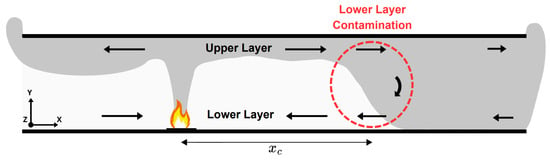
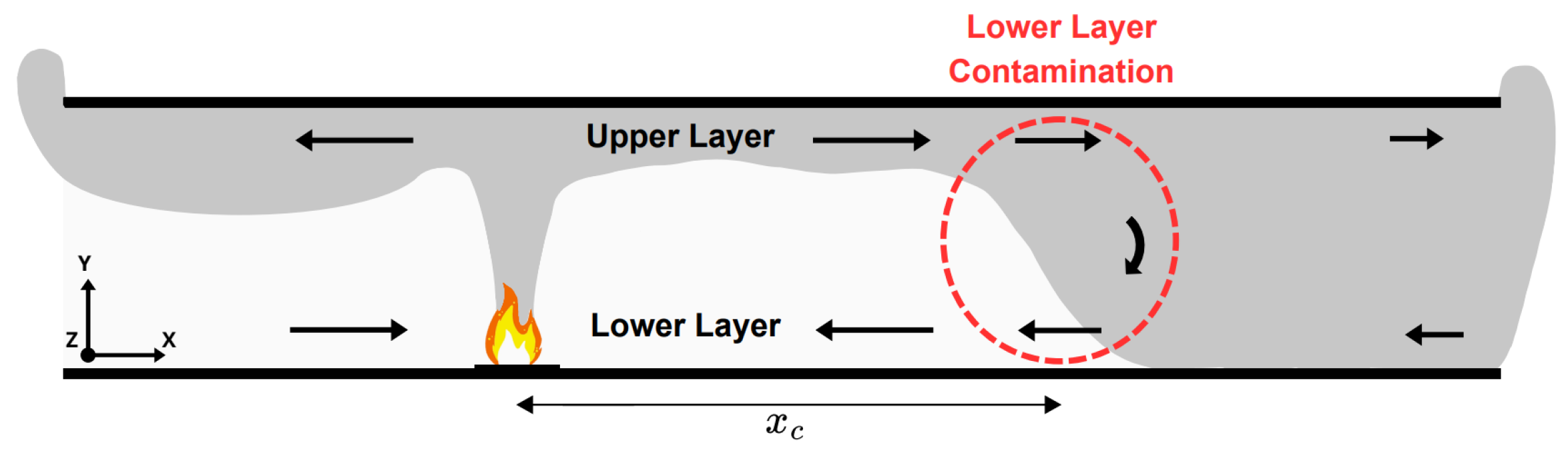
During a tunnel fire, two distinct layers form. The hot layer carries smoke from the fire source toward the tunnel portals, and a cold layer transports fresh air from outside and feeds the fire plume. These layers interact, and it is known that, at a certain distance from the fire, the cold layer becomes heavily contaminated with smoke. Once contaminated, the cold layer carries the smoke back toward the fire, eliminating any smoke-free zone. Figure 1 shows this process. Predicting this phenomenon is crucial for tunnel safety, as the main risks to human life are intoxication from toxic combustion products and loss of visibility due to soot.
Figure 1.
Flow of smoke in a tunnel.
Smoke control techniques, such as mechanical ventilation, are employed to maintain environmental conditions that ensure the safety of passengers during evacuation and firefighters during fire suppression, while minimising infrastructure damage.
However, not all tunnels require smoke control systems. Directive 2004/54/EC [1] states: “mechanical ventilation systems shall be installed in all tunnels longer than 1000 m with a traffic volume higher than 2000 vehicles per lane”. As a result, many tunnels may rely solely on natural ventilation to control smoke flow.
Hinkley [2] proposed a preliminary theory to explain the movement of hot gases within an enclosed shopping mall by applying Benjamin’s [3] theoretical investigation on the flow of gravity currents in inviscid fluids to hot, smoky gases. A set of equations was derived to calculate the depth and rate at which a layer of smoke and hot gases spreads beneath a mall’s ceiling. Although developed for malls, this theory also applies to tunnel fires. The theory comprises several sections that describe how the flow evolves under these circumstances, one of which addresses the mixing between the hot and cold layers.
One of the main factors contributing to contamination of the lower layer is buoyancy-driven flow and entrainment. Built on this, Ellison and Turner [4] developed the theory of turbulent entrainment in stratified flows, conducting a series of experiments using fresh and salt water. Later, Ingason [5] defined contamination as occurring when the Richardson number decreases below 0.8. However, more recent studies [6,7] have demonstrated that this definition alone is insufficient.
Several tests [8,9,10] have recently been carried out to improve our understanding of temperature distribution beneath the ceiling, entrainment coefficient characteristics and critical velocity variation for different HRR values. Nevertheless, the range of fire HRR investigated has been relatively low, rarely exceeding 1 MW, because full-scale tunnel fire experiments are prohibitively expensive and logistically challenging.
Advances in computational capabilities have led researchers to adopt different modelling approaches. Computational Fluid Dynamics (CFD) is the most powerful and accurate method for replacing experiments and predicting flow behaviour in tunnels. While mechanical ventilation systems have been extensively studied, natural ventilation systems have received less attention.
To address the lack of computational research in road pavements in tunnels, Caliendo et al. [11] performed numerical analyses to evaluate the effectiveness of flame-retardant (FR) asphalt mixtures in mitigating risks to occupant safety and firefighter operability during severe tunnel fires. The study modeled a 900 m long tunnel, operating under longitudinal mechanical and natural ventilation, to simulate a 100 MW fire scenario. The results demonstrated that the implementation of FR asphalt mixtures significantly improved safety conditions, resulting in a reduction in CO and concentration levels at human breathing height along the escape route and for firefighters entering the tunnel downstream of the fire under natural conditions. Nevertheless, a small number of tunnel occupants are at risk of being unable to self-evacuate.
Galhardo et al. [12] investigated a 13.5 MW fire influenced by wind, concluding that the lower layer may become contaminated with smoke as close as 138 m from the fire source. Ortega et al. [13] extended the investigation to inclined tunnels with the same firepower and found that the slope increases the likelihood of lower layer contamination compared to horizontal tunnels. However, beyond a certain slope, the stack effect causes air to enter through the lower part of the tunnel. This alters the fire and flow dynamics, affecting flame behaviour, temperature, velocity, and smoke layer thickness.
Zhang [14] conducted simulations in a 500 m tunnel with three source-ceiling heights, three tunnel widths, nine slopes, and two heat release rates, 5 MW and 7.5 MW. One of the major findings was that the smoke back-layering length decreases as the tunnel slope increases. Additionally, the study observed that the fire source heat release rate and tunnel width have no significant effect on the smoke back-layering length, but it decreases with a decrease in source-ceiling height. Yu [15] examined the combination effect of tunnel slope and longitudinal fire location on the asymmetric flow fields in a naturally ventilated tunnel. To achieve this, a total of 141 simulation cases were conducted, varying four parameters: total tunnel lengths, longitudinal fire locations, tunnel slopes, and HRRs. The study ultimately concluded that, for tunnels going uphill from left (upstream) to right (downstream) portals, the two effects are positively additive when the fire is located at the upstream tunnel, while the two effects are counteracted when the fire is located at the downstream tunnel.
The aforementioned studies, however, never considered a wide range of firepower. For reference, NFPA 502 [16] provides typical heat release rate values for different vehicle types: 5–10 MW for a passenger car; 10–20 MW for multiple passenger cars; 25–34 MW for a bus; and 70–130 MW for a heavy goods vehicle carrying burning cargo. Caliendo et al. [17] simulated fire HRR ranging from 8 to 100 MW in an 850 m long naturally ventilated horizontal tunnel and concluded that passengers would have sufficient time to evacuate safely. Later, Caliendo et al. [18] investigated the combined effects of longitudinal slope, pressure difference between the portals, and peak hourly volume on user safety in the event of a fire within a unidirectional road tunnel. The study concluded that certain combinations of these variables create an unacceptable risk level.
To ensure passenger safety, the available evacuation time must allow occupants to reach the nearest emergency exit before smoke contaminates the lower layer through which they evacuate. Specifically, if the nearest emergency exit is between the fire source and the contamination point, the safe evacuation time must be less than the sum of the time it takes for smoke to reach the contamination point and for the lower layer to carry it back to the nearest exit. This study aims to improve the understanding of the physical processes that cause lower layer contamination in naturally ventilated tunnel fires, as this is a crucial step in ensuring safety.
CFD was used to simulate tunnel fires with heat release rates ranging from 6 to 100 MW in a horizontal tunnel, both with and without wind influence. This range covers a wide variety of scenarios, from single passenger cars (HRR of about 6 MW) to heavy goods vehicles carrying burning cargo (HRR of about 100 MW), as well as combinations of different vehicle types. The results revealed that the variation in HRR needed a new method for determining the beginning of contamination, distinct from the approach previously presented by Ortega et al. [13].
However, such analyses are limited by the computational requirements of the simulations. The multitude of fire and ventilation scenarios that need to be explored adds further complexity. Furthermore, the computational cost increases with tunnel length. This cost is often impractical for engineering purposes, even for tunnels less than 500 m long.
A less expensive alternative is the use of one-dimensional (1D) models [19]. While less accurate, they provide valuable insight into the overall behaviour of the main quantities under study. Further efforts are now being directed towards hybrid approaches [20], in which CFD is applied in regions close to the fire, characterised by strong transverse and longitudinal temperature and velocity gradients, while 1D models are used in regions far from the fire where transverse gradients are negligible.
Consequently, a previously developed one-dimensional model was improved to rapidly estimate where lower layer smoke contamination begins (Galhardo et al. [12], Ortega et al. [13]). This was achieved by adopting an entrainment coefficient adjusted for varying HRR levels and implementing a new method for calculating the upper layer temperature, offering a computationally efficient alternative for engineering applications.
2. Methods
2.1. CFD Model
Several simulations were performed using the FireFOAM software package (version 1912) [21] during the course of this work. This solver was chosen due to its flexibility and physical model choices. Much of the research on CFD simulations of tunnel fires has utilized the Fire Dynamics Simulator (FDS), a commercial CFD code that uses Large Eddy Simulation (LES). Consequently, the same turbulence model was used, and results were validated using the same software.
FireFOAM is a solver within the OpenFOAM framework that is based on Favre-filtered formulations. The code uses the finite-volume method with second-order spatial accuracy and implicit time integration. The PISO algorithm was used to numerically solve the three-dimensional, Favre-filtered Navier–Stokes equations. Turbulence was modelled using LES along with the subgrid-scale Smagorinsky model. Combustion was modelled using an eddy dissipation model that assumes a global, mixing-controlled, irreversible reaction. To model radiation, heat transfer was computed under the assumption of a grey medium with negligible scattering using the finite-volume/discrete ordinates method (fvDOM). Galhardo et al. [12] provide additional details on the mathematical and physical formulation of these models.
2.2. CFD Implementation
To ensure a direct comparison with the results obtained by Galhardo et al. [12] and Ortega et al. [13], the same CFD framework was employed. This work adopted the same 1200 m tunnel geometry. However, in this case, the tunnel was considered horizontal, and the fire HRR was treated as a variable. Simulations were performed with and without the influence of wind. In addition, two 15 m extensions were added outside the portals to model the interaction between the tunnel flow and the external environment more accurately.
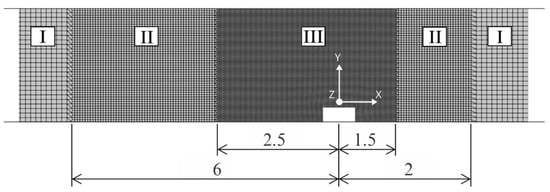
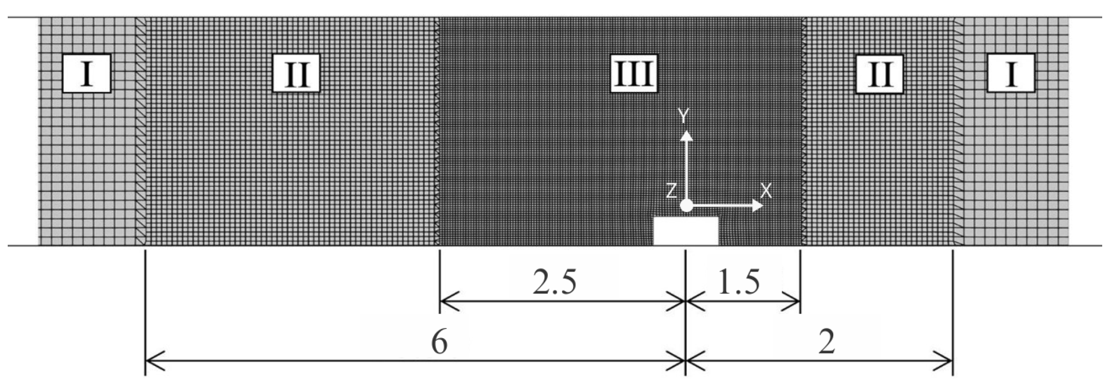
The mesh configuration consisted of three refinement regions, labelled Regions I, II, and III, whose dimensions are shown in Figure 2, along with the orientation of the axes. The grid size is = 0.08 m in the region of the thermal plume in order to obtain a Plume Resolution Index (PRI), defined as the ratio of the characteristic plume diameter to the mesh size, sufficiently high to accurately resolve the plume for all HRR and = 0.32 m in the region away from the fire, where the vertical and transverse velocities are much smaller than the longitudinal velocity. Region II serves as a transition between Regions I and III. Since the tunnel is horizontal, the extents of Regions II and III were determined under the assumption that the plume remains upright, but were elongated in one direction to account for wind effects.
Figure 2.
Mesh refinement near the fire source in simulations with wind action (dimensions in m).
To minimise computational cost, only one quarter of the tunnel was simulated in the cases without wind ( and ). In the wind cases, half of the tunnel was simulated ( was assumed as a symmetry plane). At the symmetry planes, the gradient of all variables was set to zero.
The fire source was modelled as a rectangular surface and treated as a dodecane source, with the vertical velocity calculated to match the desired heat release rate (HRR). The ambient temperature was set at 489 K, corresponding to the fuel’s boiling point. At the tunnel walls, a no-slip condition with wall functions was applied to the velocity, and a zero gradient condition was imposed on the mass fractions of the chemical species. Furthermore, heat transfer across the tunnel walls was taken into account using an overall heat transfer coefficient of . Ambient values of temperature and species mass fractions were prescribed at the open boundaries for inflow, while a zero-gradient condition was applied for outflow. The pressure deviation from the hydrostatic field, , was treated differently for inflow and outflow, as defined by the following equation:
where is the outward-pointing surface normal. The reference pressure is imposed as the static pressure in the case of outflow, and as the total pressure in the case of inflow. In the validation case, a value of was applied at both portals.
Table 1 summarises the details of all simulations performed. Here, L is the tunnel length, P is the percentage of time during which the wind velocity adopted in the simulation is exceeded, V is the wind velocity, is the pressure difference generated by the wind between the portals, and v is the average velocity of the flow inside the tunnel induced by the wind. For each heat release rate, steady state was achieved at different times after ignition. The time t refers to the instant at which the simulation was analysed.
Table 1.
Simulation parameters.
2.3. CFD Validation
Galhardo et al. [12] already validated the CFD model against the Memorial Tunnel Fire Ventilation Test Programme (MTFVTP) using a HRR of 13.5 MW and a heat source area of 9 . Since in this work different heat release rates were studied, the model was also validated by simulating Test 502 of the MTFVTP, which corresponds to an HRR of 50 MW. Details of the tunnel geometry and test conditions can be found in Bechtel and Brinckerhoff [22]. Both tests were conducted in a naturally ventilated tunnel, with the fire source represented by a pool fire of fuel oil no. 2 (modelled as dodecane).
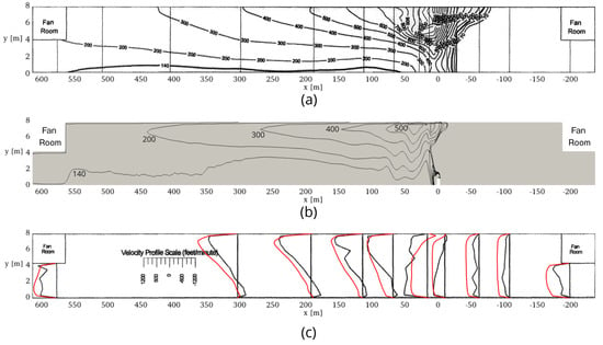
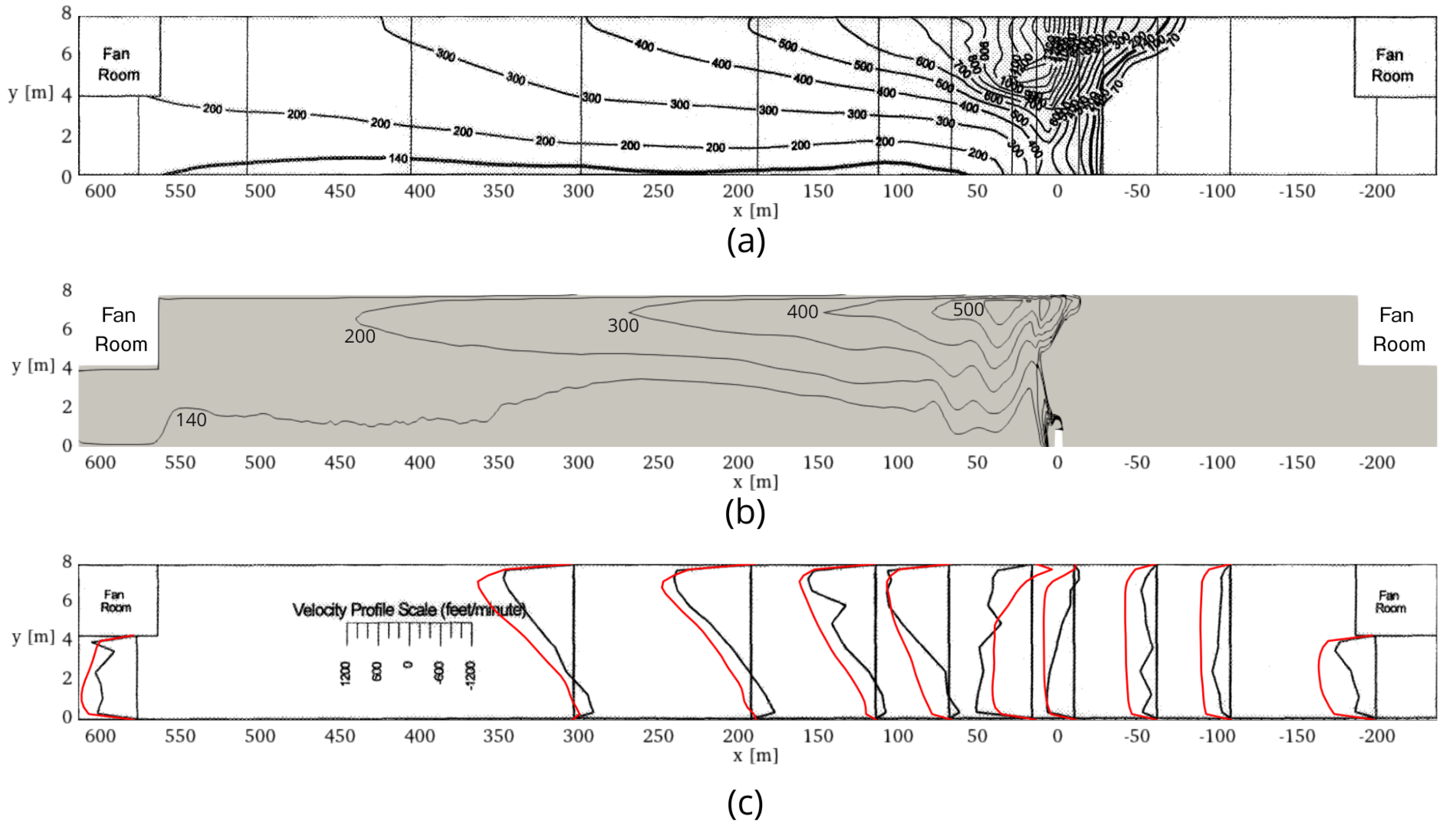
Figure 3 compares the predicted temperature field and vertical profiles of the x-velocity component with the experimental measurements from the MTFVTP test 502, taken 14 min after full pan engulfment. The tunnel’s horizontal and vertical dimensions use different axis scales for clarity. All results are presented in British units to match the experimental data in Ref. [22].
Figure 3.
Comparison of the temperature and velocity measurements obtained for the MTFVTP test 502 14 min after full pan engulfment with the CFD predictions. (a) Measured temperature contours from MTFVTP; (b) CFD predicted temperature contours; (c) Predicted (red lines) and measured in the MTFVTP (black lines) x-velocity vertical profiles.
Some discrepancies were observed between the experimental and numerical results, particularly with regard to the temperatures measured farther from the heat source. These discrepancies can be attributed to the simplifications made when implementing the physical models and the approximation of parameters such as heat transfer across the tunnel walls, as well as the use of dodecane with fixed soot yields. Additionally, the limited experimental data, which were only measured along the vertical lines shown in the figure, required interpolation to describe the temperature distribution throughout the tunnel, introducing uncertainties in the experimental results. Furthermore, comparing the experimental and numerical velocity profiles shows that the CFD model can produce reasonable predictions of the longitudinal velocity field. Overall, the CFD model has proven effective in simulating the large-scale behaviour of the ceiling jet in this tunnel fire scenario.
3. Simulation Results
The main objective of this work is to improve our understanding of how smoke from the upper layer contaminates the lower layer, specifically by determining the distance from the fire source to the point at which contamination begins. To achieve this purpose, several simulations were conducted in a horizontal tunnel with heat release rates ranging from 6 MW to 100 MW, both with and without external wind action.
All simulations were run until a steady state was reached. To further investigate lower layer contamination, several quantities were evaluated. The interface separating the two layers was defined as the surface where the flow velocity is zero (), with the cold layer moving from the tunnel portals towards the fire source and the hot layer moving from the fire source towards the portals. The average temperature, velocity, and mass flow rate were calculated at tunnel cross-sections spaced every 10 m. The average mass flow rate was obtained by integrating the mass flux over each cross-section.
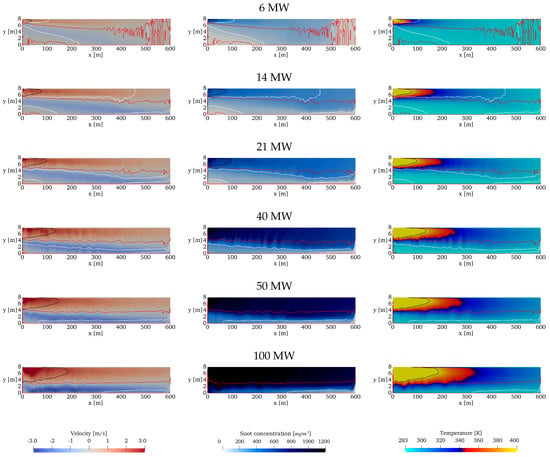
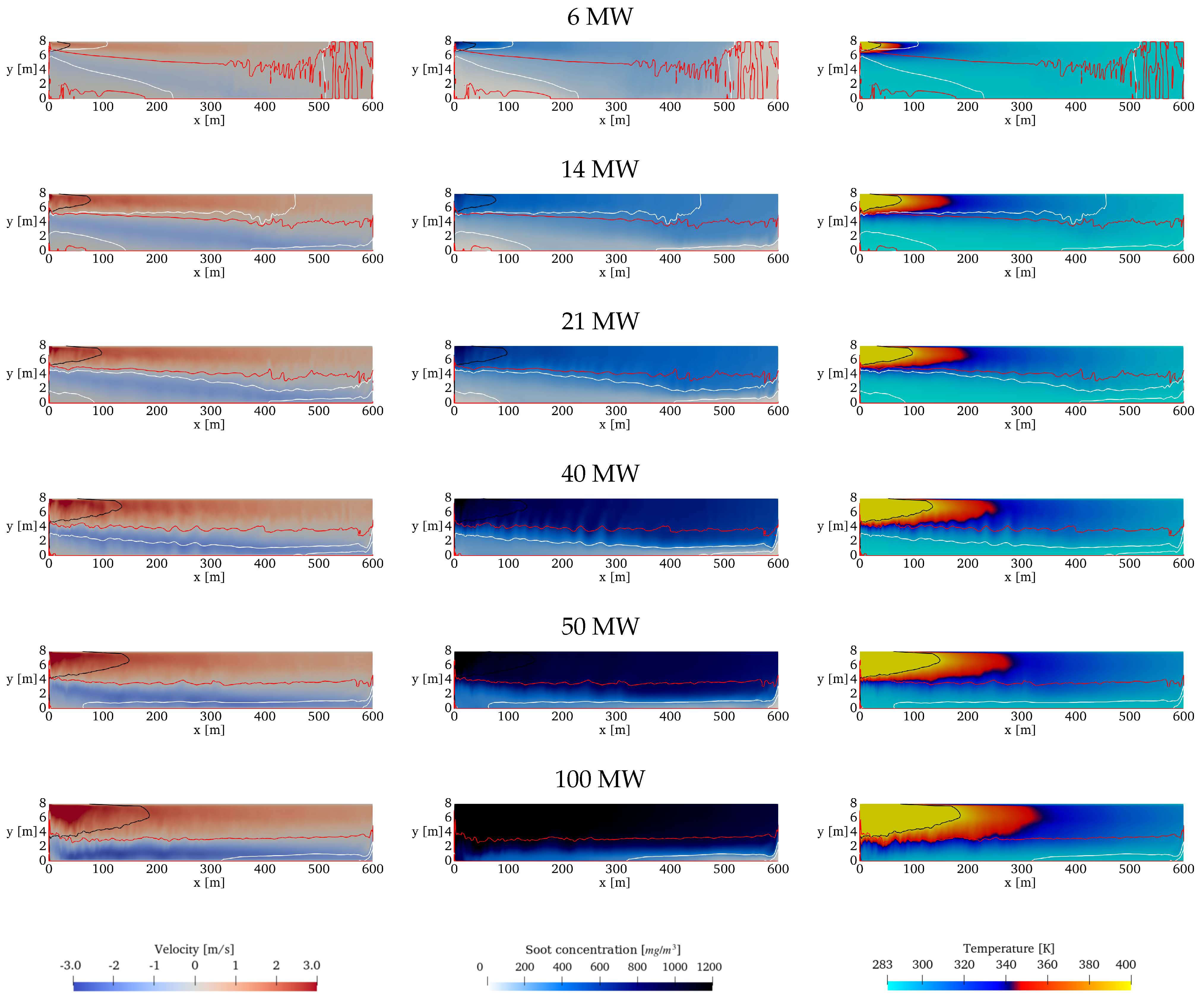
Figure 4 presents the predicted velocity magnitude, soot concentration, and temperature for all fire HRRs at steady state and without wind. The red line corresponds to zero velocity, representing the boundary between upper and lower layers. The white lines indicate soot concentrations of 80 mg/m3 and 300 mg/m3, which correspond to visibility distances of 5.0 m and 1.3 m for reflecting signs, respectively. The black lines correspond to a temperature of 127 °C.
Figure 4.
Steady-state fields of velocity magnitude, soot concentration, and temperature for different HRR simulations.
Figure 4 shows that increasing HRR leads to higher temperatures and velocities, as expected. For all HRR levels, the line separating the two layers (red line) appears to stabilise at a height slightly below 4 m as the distance from the fire source increases. This provides a similar cross-sectional area for both layers and is consistent with a horizontal tunnel without wind. In this scenario, both layers carry the same mass flow rate, and the temperatures of the two layers also become closer to each other far from the fire source. In contrast, the white lines progressively shift downwards. The velocity difference at the interface between the upper and lower layers increases, intensifying shear forces. This leads to greater mixing and increased smoke transport to the lower layer. As a result, smoke concentration rises and visibility is significantly reduced. In the 100 MW case, the minimum clear-layer height is approximately 1 m.
For the 6 MW case, the line separating the two layers behaves differently than at other HRR levels. In this case, the HRR is so low and the velocities so weak that the hot layer remains confined within the tunnel. Beyond 500 m, the line is no longer continuous, indicating an absence of a well-defined interface between the two layers. Therefore, this case is treated separately in the following sections.
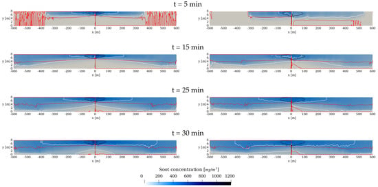
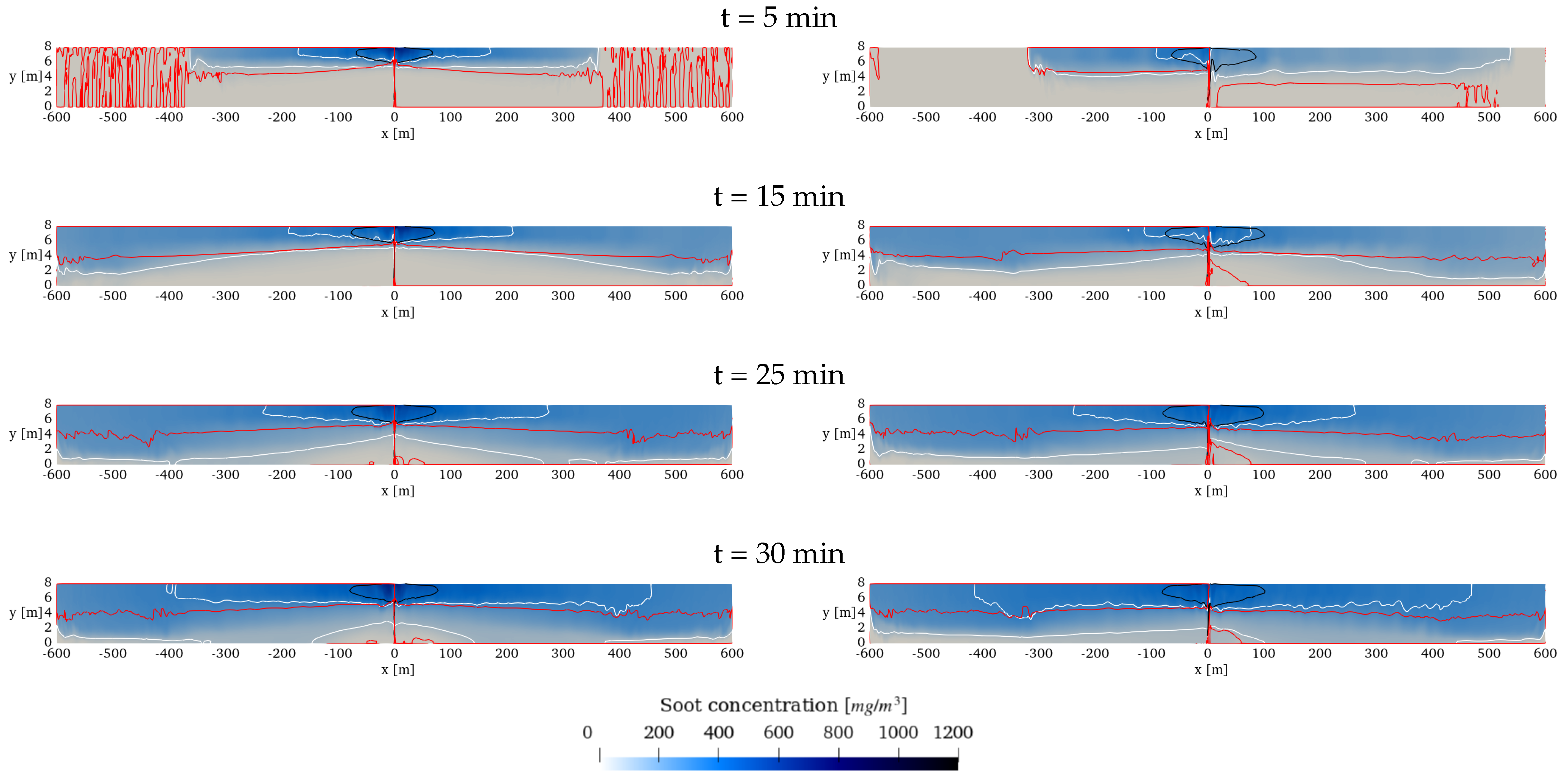
Figure 5 shows how wind affects lower layer contamination for the 14 MW case. At 5 min, the wind breaks the symmetry by pushing smoke toward the left portal and promotes its exit through the right portal. At later times, such as 30 min, the influence of the wind is reflected in higher smoke concentrations on the left side. This is shown by the downward shift of the 300 mg/m3 white line compared to the windless case.
Figure 5.
Comparison of the evolution of soot concentration for a 14 MW fire without wind (left) and with a wind velocity of 0.77 m/s (right).
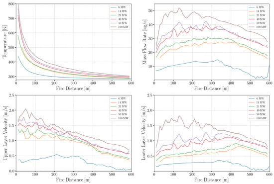
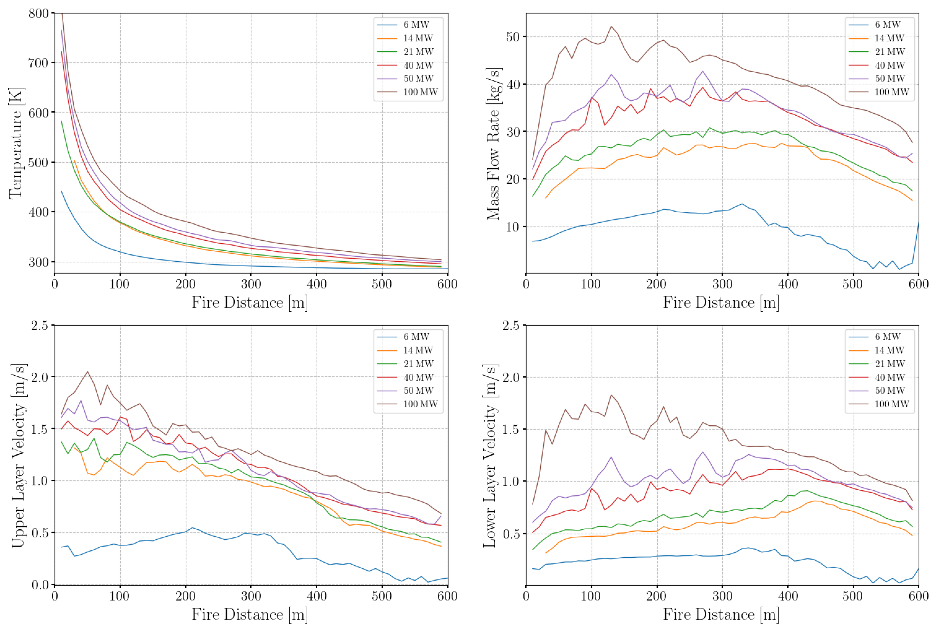
Figure 6 provides better insight into how the variables evolve quantitatively as the distance from the heat source increases. As can be seen, the higher the HRR, the greater the values of all the variables. Excluding the 6 MW case, the variables exhibit similar trends as the distance from the fire source increases: the temperature and velocity of the upper layer decrease continuously, while the mass flow rate and velocity of the lower layer initially increase before decreasing.
Figure 6.
Quantities, obtained by CFD simulations, related to the lower layer contamination with smoke during tunnel fires without the wind effect.
The continuous decrease in the mass flow rate of the upper layer beyond a certain distance from the heat source indicates contamination of the lower layer. As HRR increases, the contamination of the lower layer occurs closer to the heat source. It is also observed that, as the distance from the heat source increases beyond the start of contamination, the velocities of both layers follow the same trend. However, even though both layers transport approximately the same mass flow rate and their temperatures become more similar farther from the fire source, the lower layer velocity remains slightly higher. This occurs because the interface between the layers lies slightly below 4 m, resulting in a smaller cross-sectional area for the lower layer, which leads to a higher velocity.
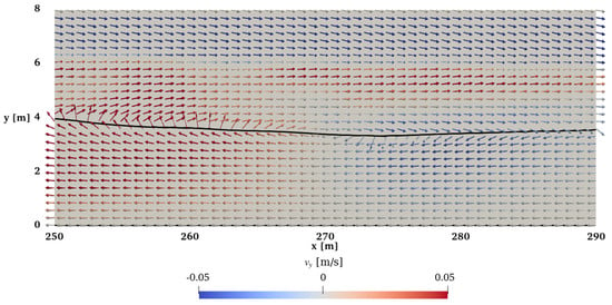
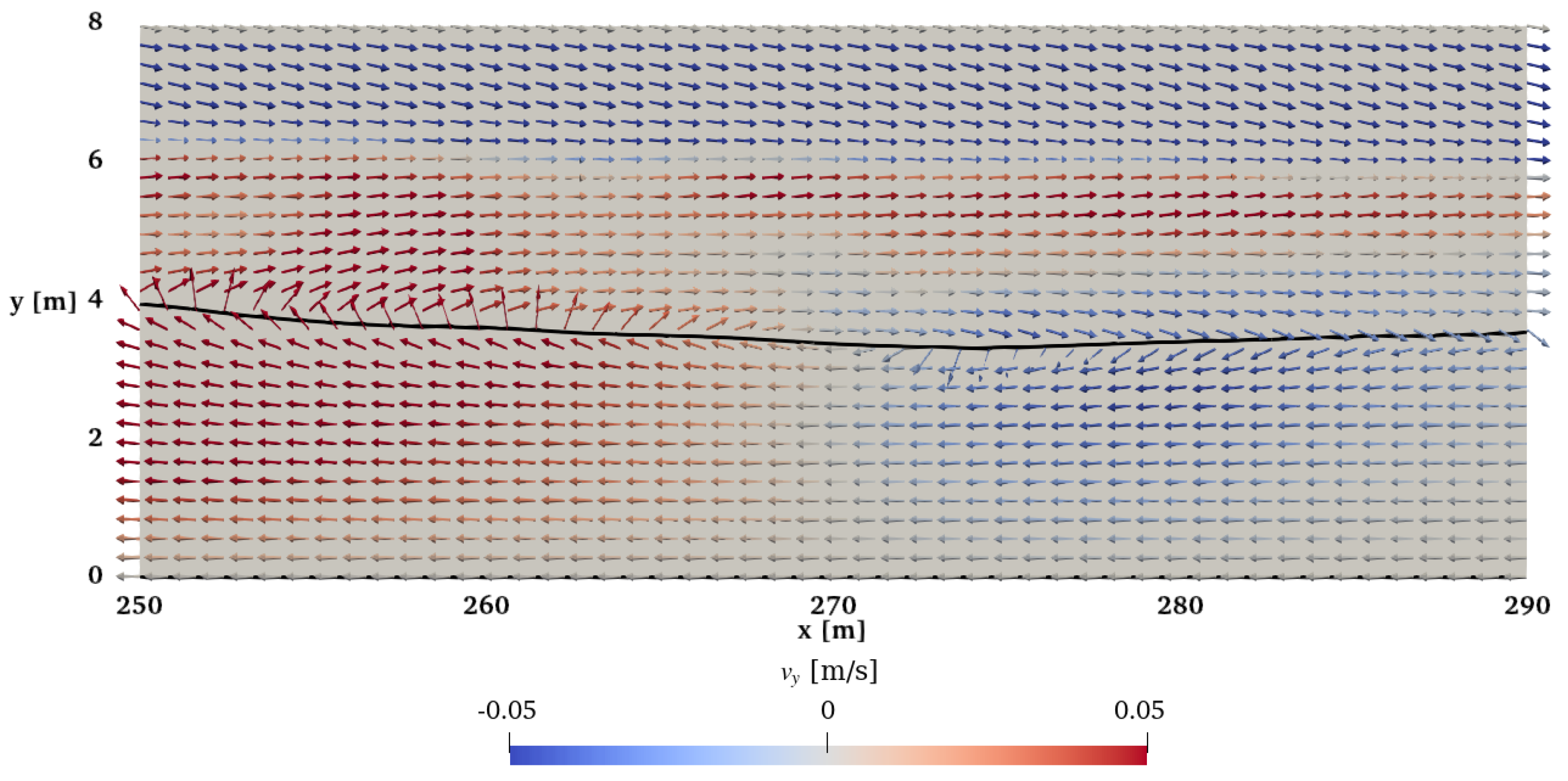
As the HRR increases, vortices have a stronger effect, as seen in more pronounced curve fluctuations. Figure 7 shows the velocity vector field near the peak mass flow rate for the 50 MW case. The direction of the vectors shows the mean velocity, while their colour represents the magnitude of the mean velocity y-component. A vortex is clearly visible in this image and is responsible for the mass transfer between the layers. On the left, transfer occurs from the lower to the upper layer, shown by vectors pointing upward at the interface. The opposite occurs on the right side.
Figure 7.
Mean velocity vector field in the region of the peak mass flow rate for the 50 MW case.
4. Discussion
4.1. General
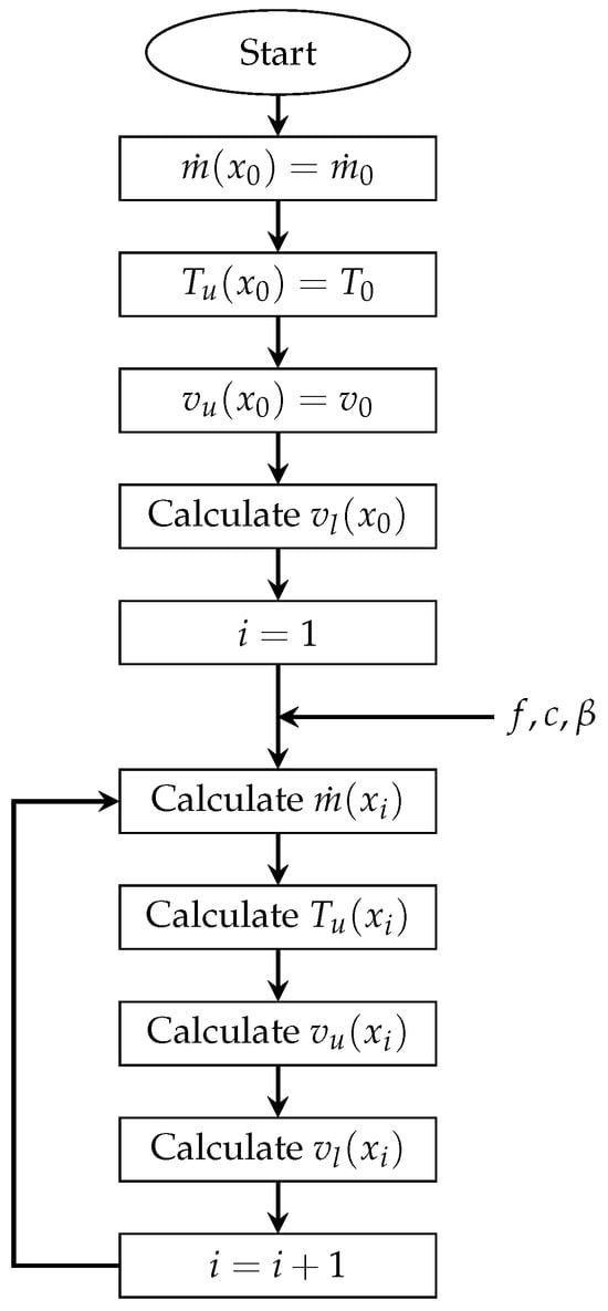
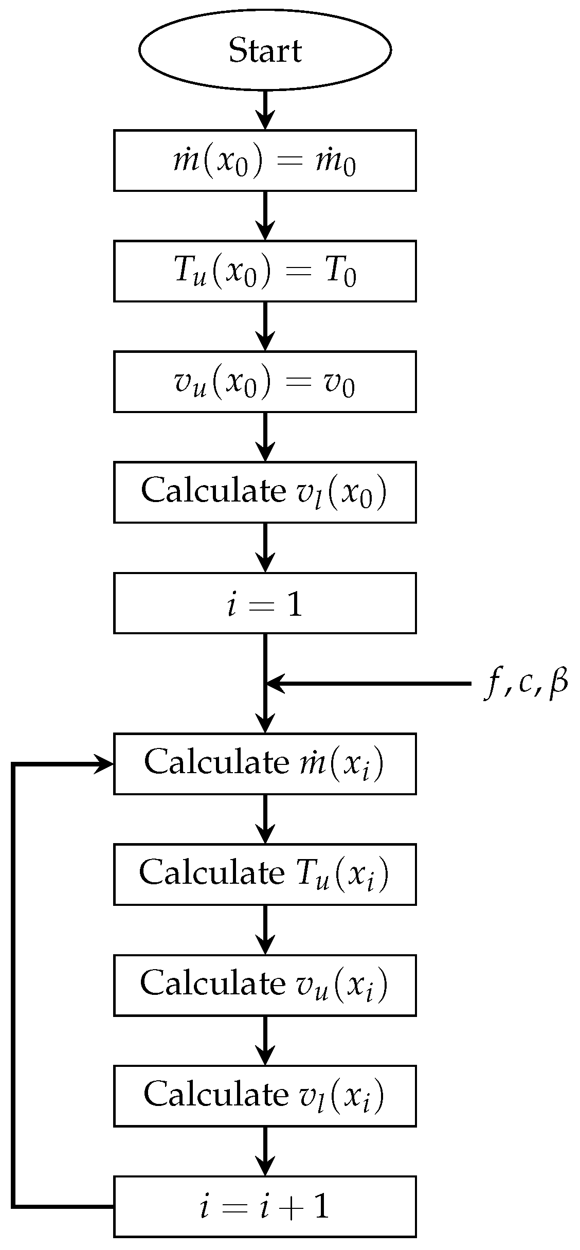
Following the approach reported by Galhardo et al. [12] and Ortega et al. [13], a one-dimensional semi-analytical model was developed. This model assumes strictly one-dimensional flow in the x-direction. Necessary input data, such as the initial mass flow rate and upper layer temperature, were obtained directly from the CFD simulation, while the initial upper layer velocity and the coefficients , and were estimated via the least squares method applied to simulation results. Figure 8 illustrates the algorithm used to implement the 1D model.
Figure 8.
One-dimensional model algorithm.
Unlike Hinkley’s theory [2], which assumed that mixing would not become significant until the hot gas layer had cooled enough for density differences to be negligible except for buoyancy effects, the present model explicitly accounts for temperature differences. It predicts the contamination point based on a physical limit.
The upper layer mass flow rate is calculated without considering the confinement effect. Only the entrainment of fluid from the cold layer into the hot layer is considered. As a result, the predicted upper layer mass flow rate increases continuously with distance from the fire source. However, buoyancy effects create a physical limit that prevents the upper layer velocity from increasing beyond a certain limit, and the upper layer mass flow rate from growing indefinitely. When this limit is surpassed, contamination of the lower layer begins.
The model currently only evaluates steady state cases and is not yet fully predictive. Instead, it is a preliminary step toward an algebraic formulation that can predict where lower layer smoke contamination starts.
Galhardo et al. [12] studied a horizontal tunnel exposed to wind. Ortega et al. [13] investigated the impact of tunnel slope on the same tunnel design and heat release rate. This study re-evaluates the previously developed 1D model. It uses the same horizontal tunnel while testing different fire heat release rates, combined with wind. The set of balance equations for the model is shown below [5,23]:
where and are the temperatures of the external air and the tunnel walls, respectively, is the mass flow rate of the upper layer, is the specific heat in , is the density of the external air, is the entrainment velocity, the wet perimeter, and W is the width of the interface between the upper and lower layer. In Equation (3), is the area of the cross-section of the upper layer, is the slope of the tunnel, g is the acceleration of gravity, and is the upper layer hydraulic diameter.
The next sections compare CFD results and 1D model estimates to clarify the influence of key variables on smoke motion and contamination in tunnel fires.
4.2. Upper Layer Mass Flow Rate
The upper layer mass flow rate () can be derived by integrating the continuity Equation (2) between two cross-sections:
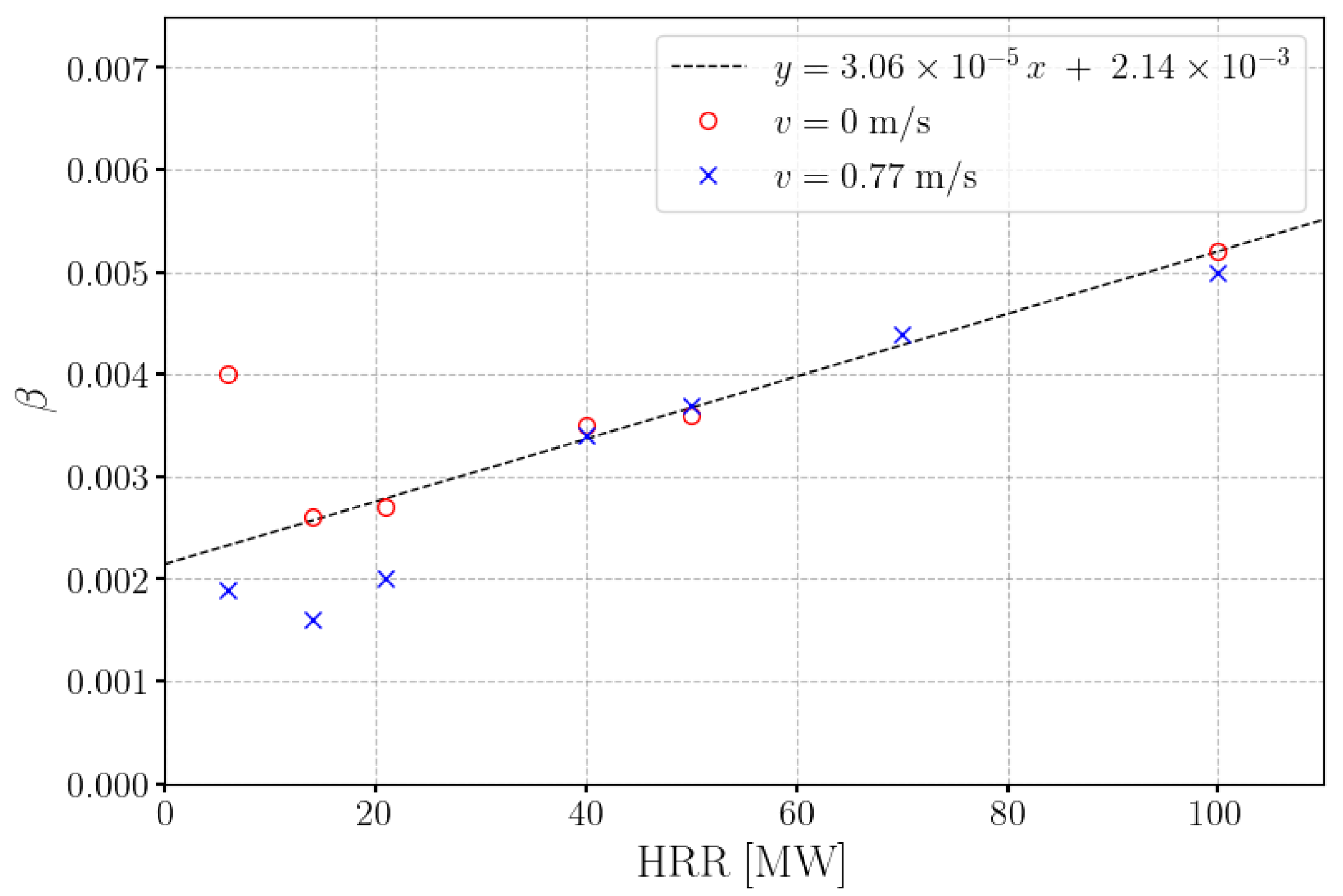
where is the initial mass flow rate, which was directly obtained from the simulation, and represent the mean velocities of the upper and lower layers, respectively, and is the entrainment coefficient. Although Jiang [10] derived an equation with a varying entrainment coefficient along the tunnel, the results were limited, indicating the need for further research. Thus, was assumed constant throughout the tunnel and was calculated using the least squares method.
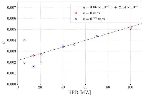
Figure 9 shows that varies linearly with increasing HRR, a trend previously reported [9]. As HRR increases, the velocity difference between the two layers also rises, enhancing shear force at the interface and intensifying air entrainment. When the wind effect was included, decreased at lower HRR levels compared to the case without wind.
Figure 9.
Best fit obtained using the least squares method, with and without wind, and the linear regression that best describes the evolution of the entrainment coefficient.
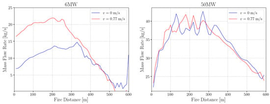
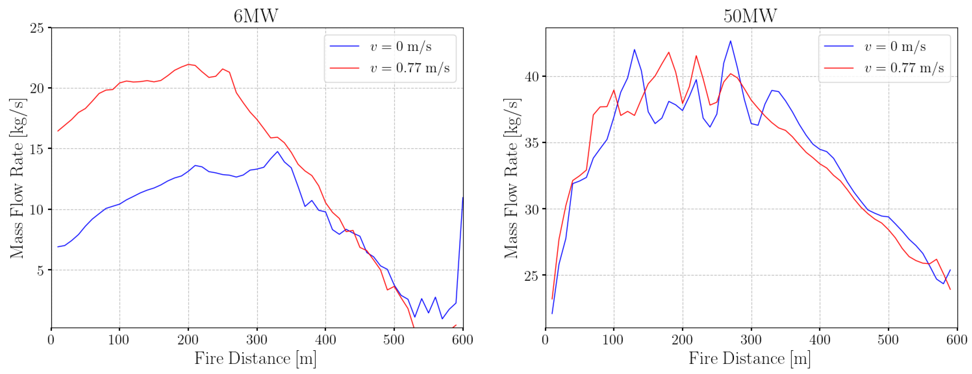
Figure 10 illustrates the difference between the upper mass flow rates with and without wind. For lower HRR the growth of the hot layer is more intense without wind, resulting in a lower value of in the wind case. For higher HRR, the effect of the wind on the evolution of the mass flow rate is less significant.
Figure 10.
Comparison between the upper layer mass flow rates obtained from the CFD simulations without wind and with a wind velocity of 0.77 m/s.
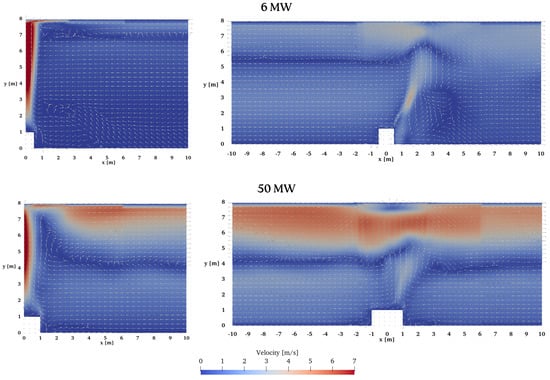
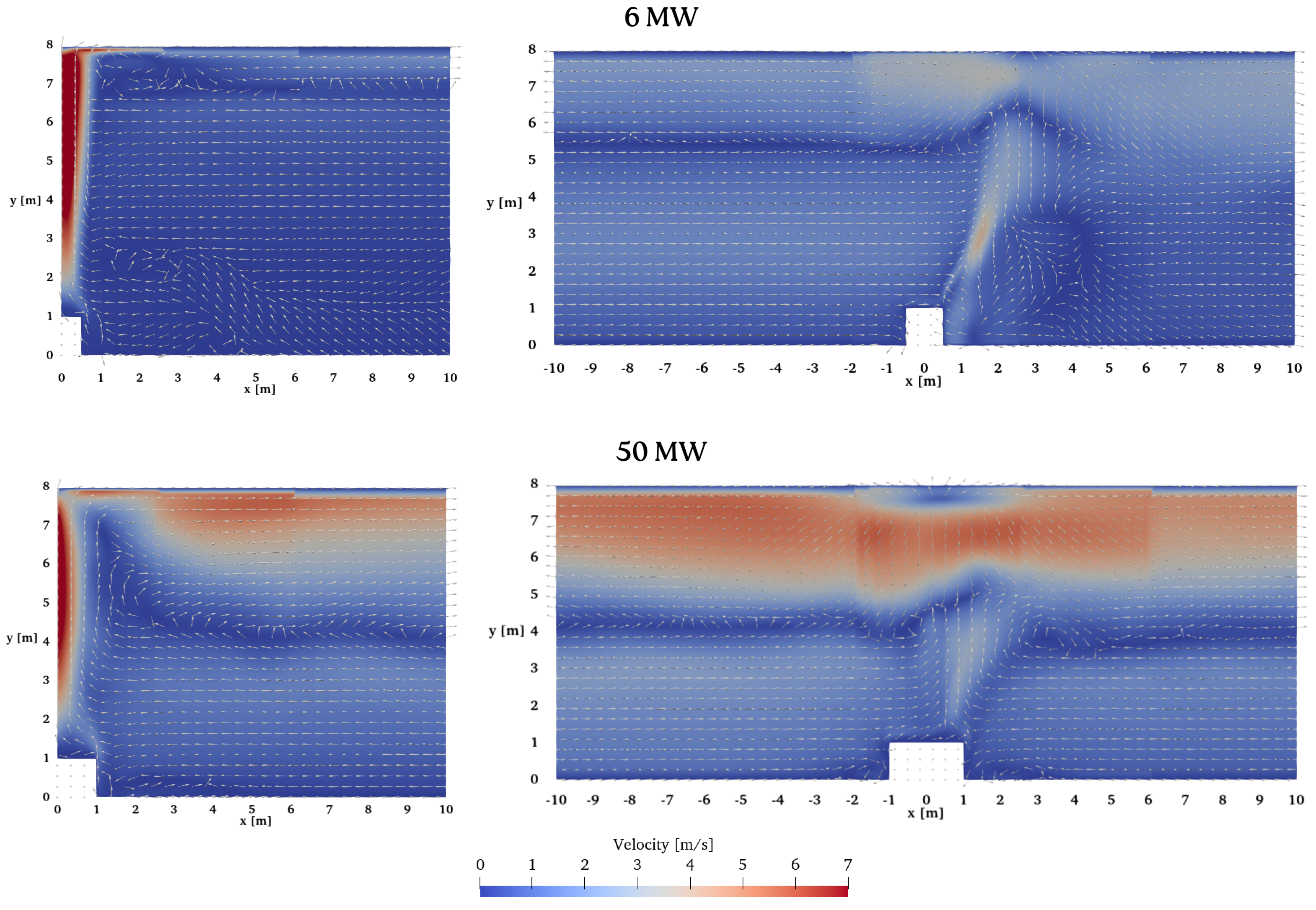
Wind has the most noticeable impact on the initial value of the mass flow rate, . With wind, the mass flow rate increases due to the immediate interaction between the thermal plume and the external flow, causing earlier entrainment into the hot layer. Figure 11 illustrates this phenomenon, showing that the thermal plume has lower velocities when wind is present.
Figure 11.
Comparison of the velocity field near the heat source without wind (left) and with a wind velocity of 0.77 m/s (right).
Additionally, plume entrainment is more significant at lower HRR, where smaller pressure differences create lower velocities. This makes the plume and the region near the fire source more affected by wind, increasing fluid entrainment into the upper layer. Higher HRR creates larger pressure differences and reduces wind influence.
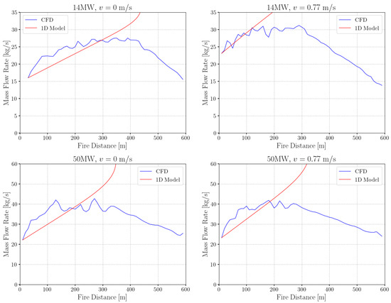
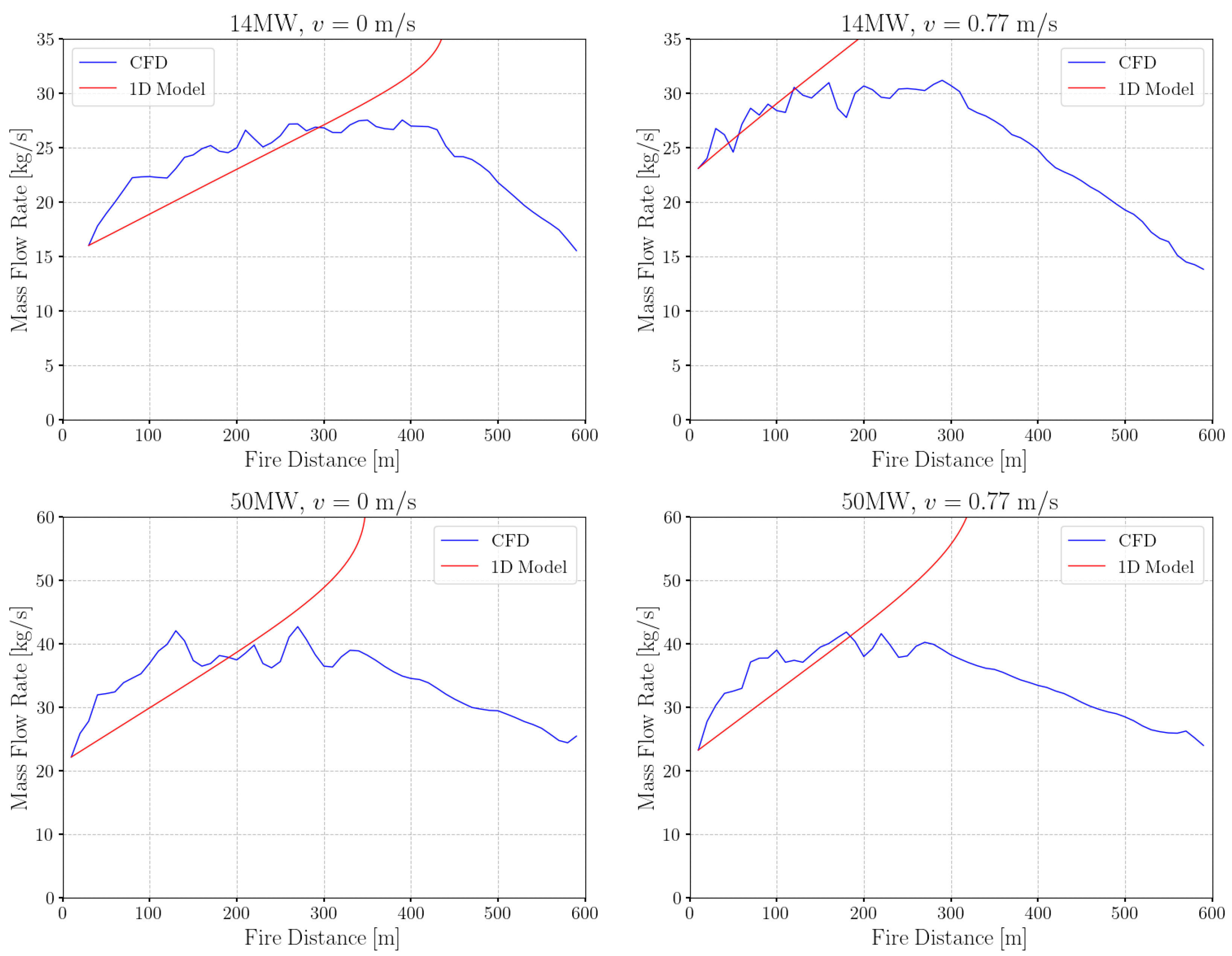
Figure 12 shows that the upper layer mass flow rate determined from the 1D model fails to capture the plateau that characterizes the upper layer mass flow rate in the region where the contamination point is approached. This is because the entrainment coefficient is considered constant along the tunnel, which restricts the rate at which the upper layer increases. Additionally, the assumption that mass transfer always occurs from the cold layer to the hot layer makes it impossible to accurately estimate the upper layer mass flow rate beyond the contamination point. However, it will later be shown that this simple model is still able to predict the distance from the heat source at which the strong contamination of the lower layer with smoke begins.
Figure 12.
Comparison between the mass flow rates at the upper layer determined from the 1D model and the CFD simulations for 14 MW and for 50 MW, either with or without wind.
4.3. Upper Layer Temperature
The upper layer temperature, , averaged over a cross-section of the tunnel, can be predicted using the following equation derived from the energy balance in Equation (4):
The variable is the convective heat transfer coefficient, which may be estimated from the following correlation [23]:
where is the Prandtl number and f is the friction factor of the tunnel wall. The friction factor, initially calculated using the least squares method, ranged from 0.0188 for 100 MW to 0.0297 for 50 MW. Ortega et al. [13] reported a similar range, 0.020 to 0.035. Since this factor is specific to the tunnel and not the HRR, it is reasonable to treat it as constant for all HRR values. The mean value obtained, , was used in the model, producing good results. This is consistent with the value reported for tunnels with concrete walls [23].
The first term on the right-hand side of the Equation (6) represents the energy losses due to mass exchange in the shear layer between the upper and lower layers. The second and third terms correspond to energy losses due to convection with the tunnel walls and radiation, respectively. It was assumed that the wall temperature was equal to the external air temperature. This assumption does not compromise accuracy because, in the region of the contamination point, far from the heat source, temperatures remain low during the initial minutes of the simulation.
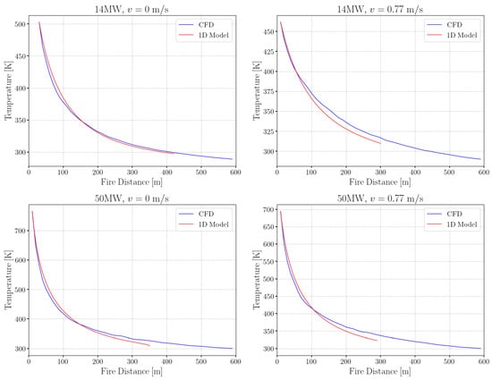
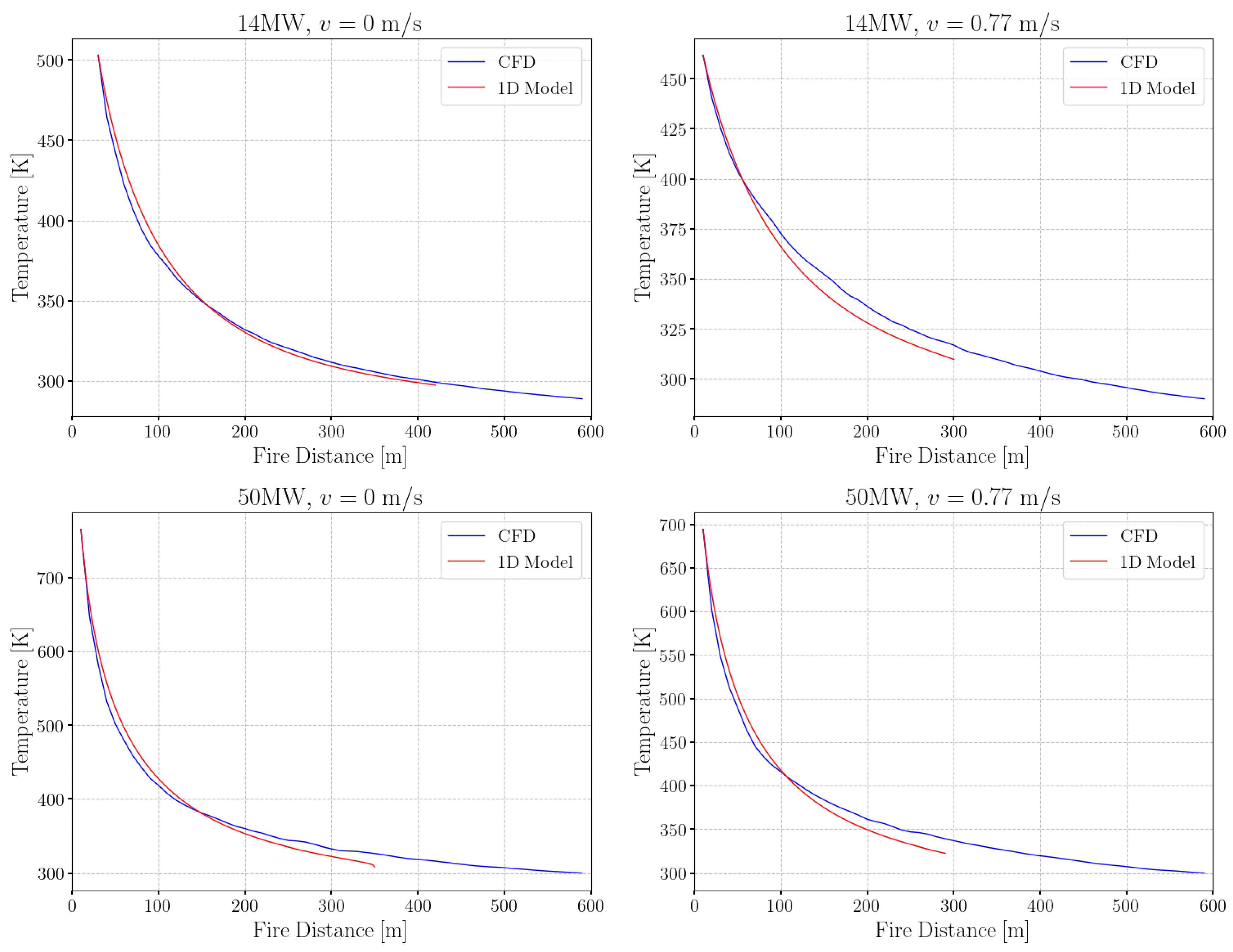
The evolution of the upper layer average temperature along the tunnel follows a hyperbolic pattern, as shown in Figure 13. The 1D model correctly predicts the temperature evolution near the heat source but consistently underestimates simulated values near the contamination point. This effect grows with increasing HRR. The reason is the flow rate calculation method. As the contamination point is approached, the 1D model predicts higher mass flow rates than the CFD simulations, and this discrepancy is more pronounced at higher HRR levels. Consequently, the energy losses due to mass exchange between the upper and lower layers are overestimated, leading the 1D model to predict lower temperatures than the CFD simulations.
Figure 13.
Comparison between the upper layer average temperature calculated from the 1D model and CFD simulations for 14 MW and 50 MW, either with or without wind.
4.4. Upper Layer Velocity
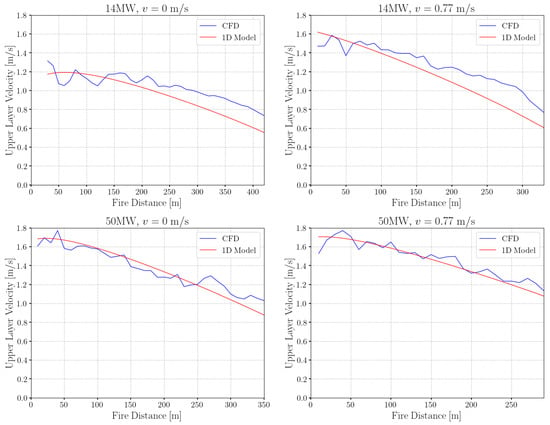
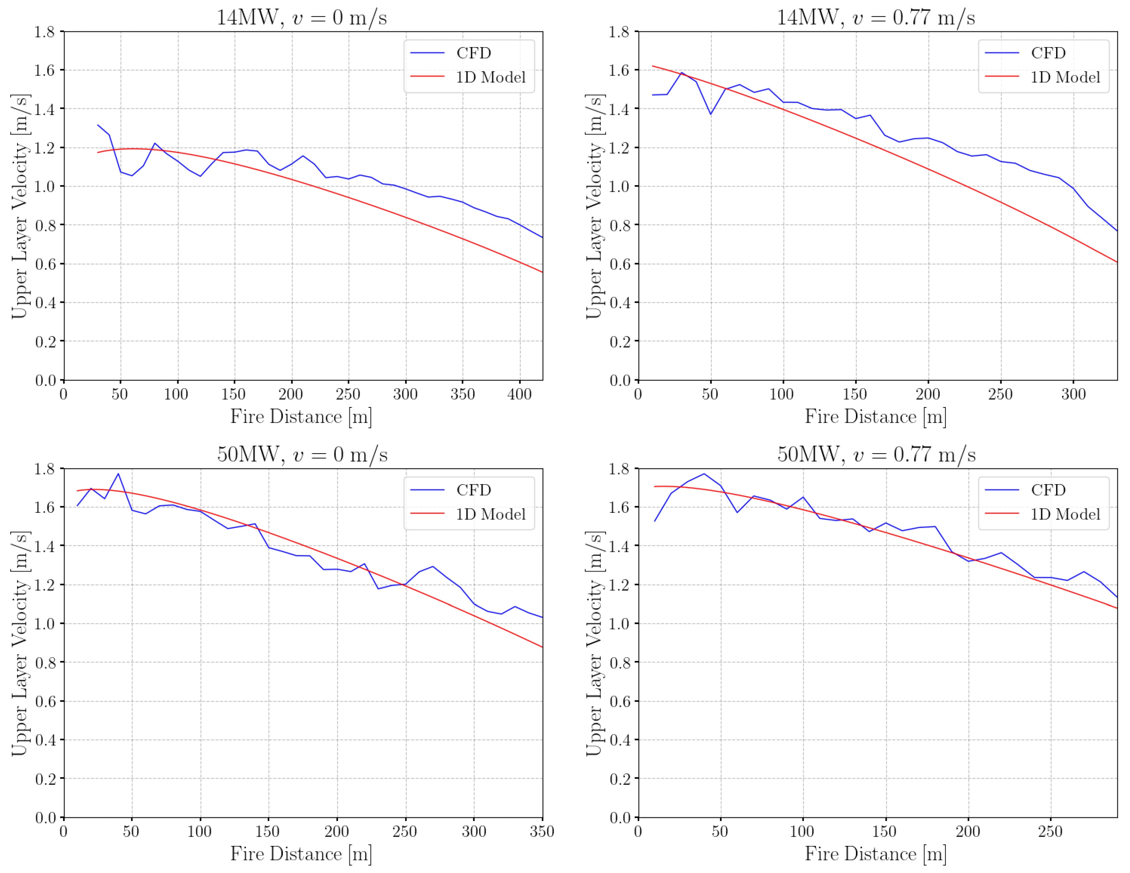
The upper layer average velocity, , is estimated using the following equation derived from the momentum balance, Equation (3) [13]:
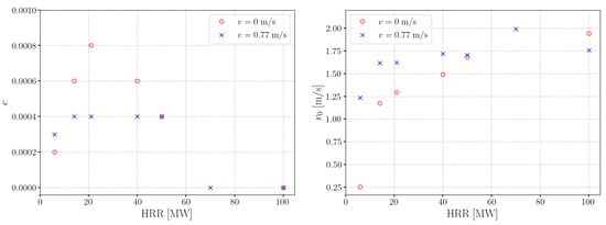
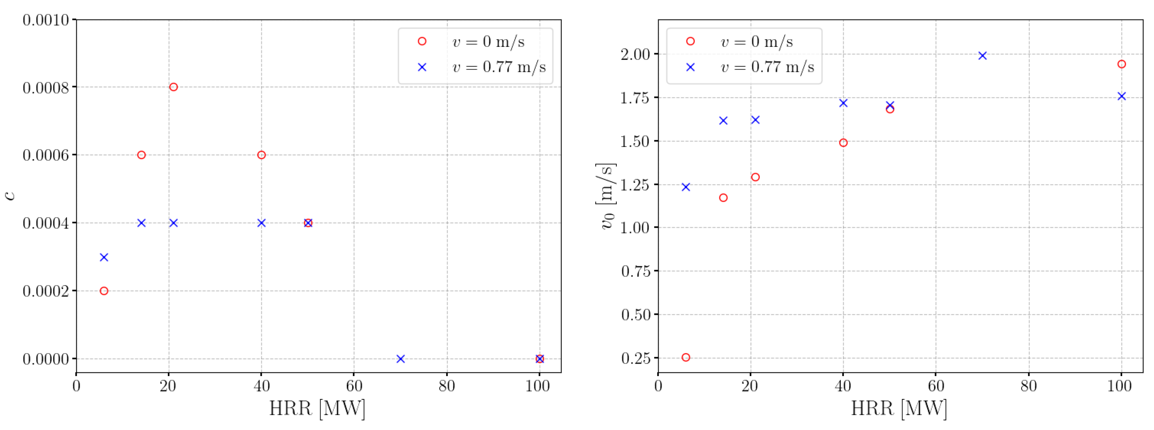
The first term on the right-hand side of the Equation (8) is the momentum source due to buoyancy. A proportionality constant related to the momentum source due to buoyancy, c, has been introduced to enable this term to be weighted when determining the best fit to the simulation results. The second term is related to the friction losses in the tunnel walls, ceiling, and shear layer (between the upper and lower layers). The initial velocity, (x = 10 m), and the coefficient c, are obtained using the least squares method. Figure 14 shows the results of the best fit obtained using this method, and Figure 15 compares the upper layer average velocity determined from the 1D model and the CFD simulations for 14 MW and for 50 MW, either with or without wind.
Figure 14.
Best fits of constant c and upper layer average velocity at x = 10 m obtained by the least squares method.
Figure 15.
Comparison between the upper layer average velocities determined from the 1D model and the CFD simulations for 14 MW and for 50 MW, either with or without wind.
The parameter c lies in the range of 0 to 0.0008. This is about two orders of magnitude smaller than values obtained by Ortega et al. [13] for sloped tunnels. In the present case, the tunnel is horizontal. Therefore, the buoyancy effect is weaker, as it relates only to the thickness of the hot upper layer and not to the difference between the heights of the tunnel portals. The results of the least squares method indicate that the initial velocity increases with higher HRR levels, due to stronger buoyancy forces. On the other hand, the wind has a significant impact only in the region close to the fire source for low HRR, leading to an increase in the initial velocity, .
4.5. Lower Layer Velocity
The lower layer average velocity was calculated using the following equation:
where is the lower layer mass flow rate, A is the total cross-sectional area of the tunnel, and v is the wind velocity. This equation shows two contributions to the average velocity of the lower layer. The first term under the square root corresponds to the lower layer velocity without wind, obtained from the mass balance in the upper and lower layers. The second term represents the flow induced by the wind in the absence of fire.
4.6. Origin of the Lower Layer Contamination
The average velocities of the upper and lower layers can be used to determine at which point it becomes physically unrealistic to consider the flows as distinct without significant mixing. Both flows are driven by buoyancy. The maximum velocity difference between the layers results from buoyancy effects. This difference can be predicted using the following equation [13], where the height of the upper layer, , was approximated by the ratio of the upper layer area to tunnel width.
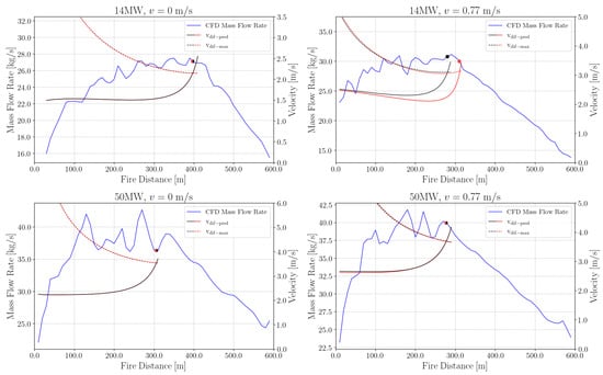
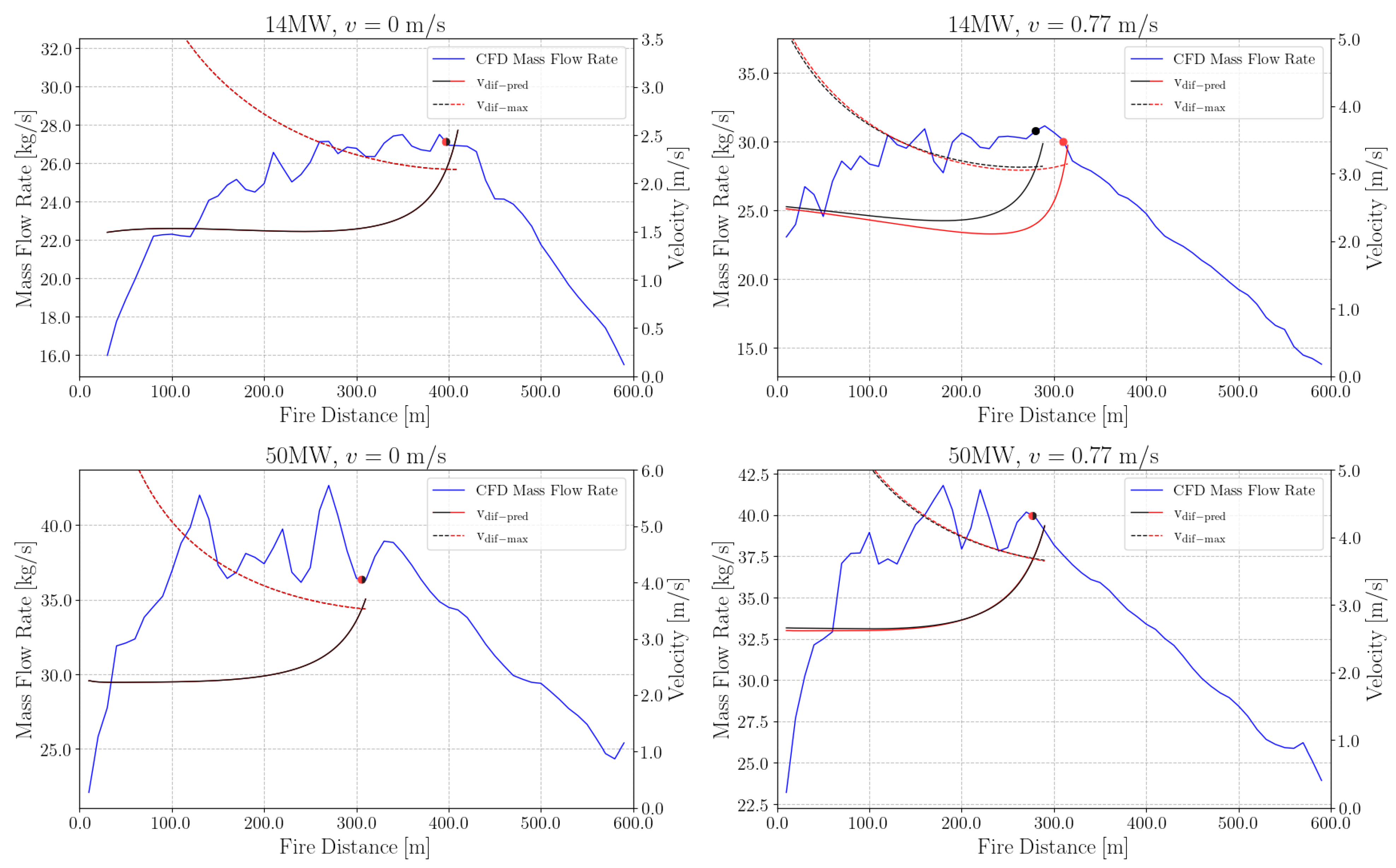
Therefore, the distance from the fire source where contamination of the lower layer begins, , corresponds to the location at which , where and . The velocity is calculated from integration of Equation (8), while and are obtained from Equations (9) and (10), respectively. At that distance from the fire source, namely beyond , it is not possible to increase the upper layer mass flow rate further because the buoyancy is insufficient. Therefore, the only physical solution is transferring mass from the upper layer to the lower layer.
According to Equation (5), the upper layer mass flow rate depends on the entrainment coefficient. Figure 16 compares the point where contamination of the lower layer begins, obtained by two different methods. The first method is marked by a black dot and uses the entrainment coefficient, , obtained from the regression line in Figure 9. The second uses the values calculated from the least squares method, marked by a red dot.
Figure 16.
Comparison of the point where contamination of the lower layer begins, obtained using the parameter determined through linear regression (black lines), and derived from the least-squares method with the friction coefficient, f, fixed (red lines).
The upper layer mass flow rate predicted by the 1D model agrees more closely with the CFD results when is calculated directly using the least squares method. However, contamination of the lower layer, marked by a decrease in the upper layer mass flow rate, is predicted more accurately when is obtained from linear regression. Therefore, this latter approach was adopted in this work.
Ortega et al. [13] assumed that the contamination point corresponds to the location where the upper layer mass flow rate reaches its maximum. However, this is not accurate at higher heat release rates. Larger vortices at high HRR levels increase fluctuations in the upper layer mass flow rate, affecting the plateau near the contamination point. Thus, the location of maximum mass flow in the upper layer may deviate significantly and unpredictably from the start of the contamination zone. Therefore, an alternative method was needed.
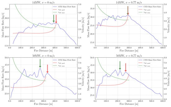
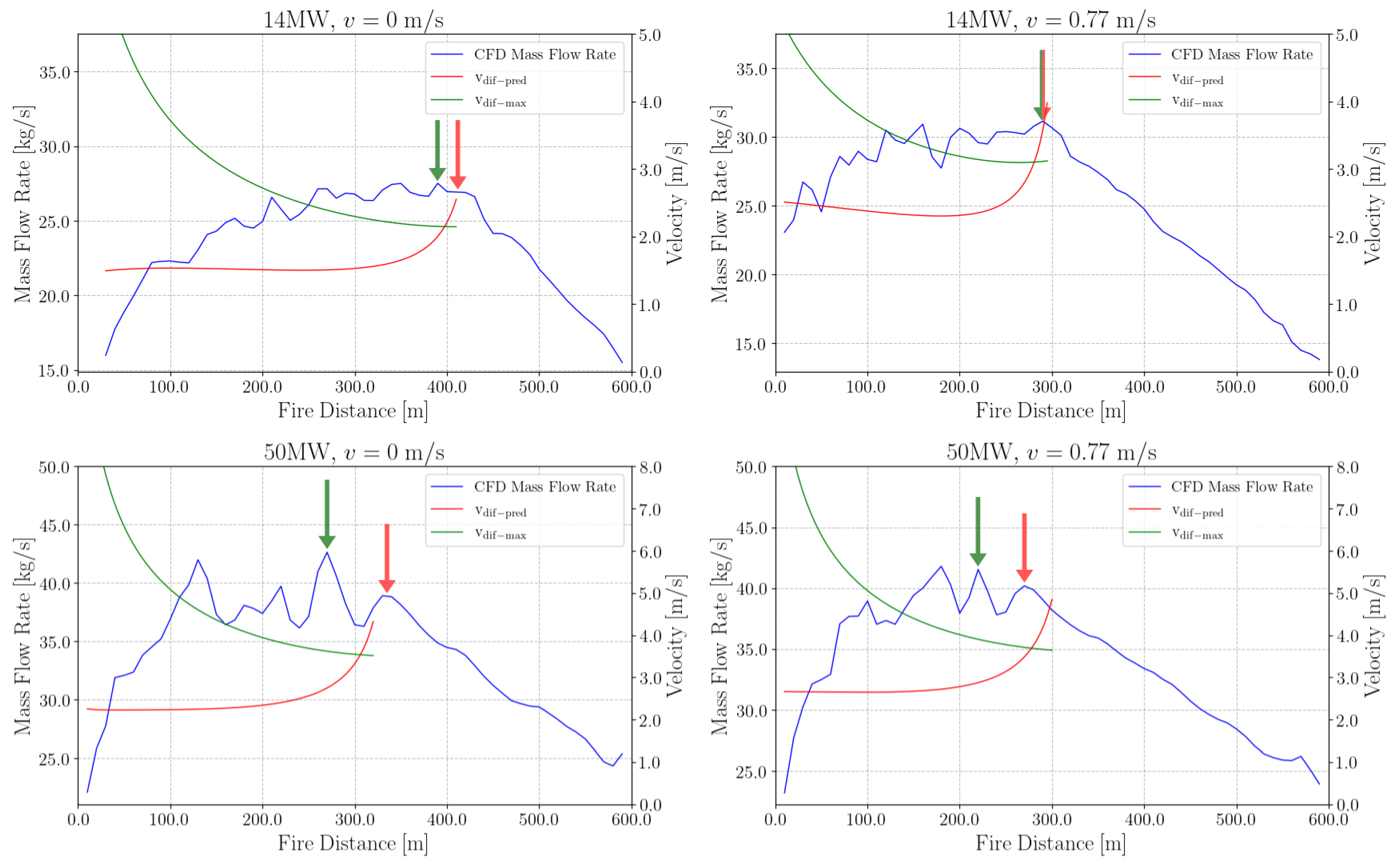
Figure 17 compares two new approaches for determining the distance from CFD simulation, using 1D model values. The first approach (red arrow) defines the contamination point as the location where the decrease in the upper layer mass flow rate first approaches an approximately constant slope. The second approach (green arrow) defines the contamination point as the first peak before the slope becomes constant.
Figure 17.
Illustration of the two different methods to define the beginning of the contamination of the lower layer.
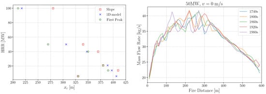
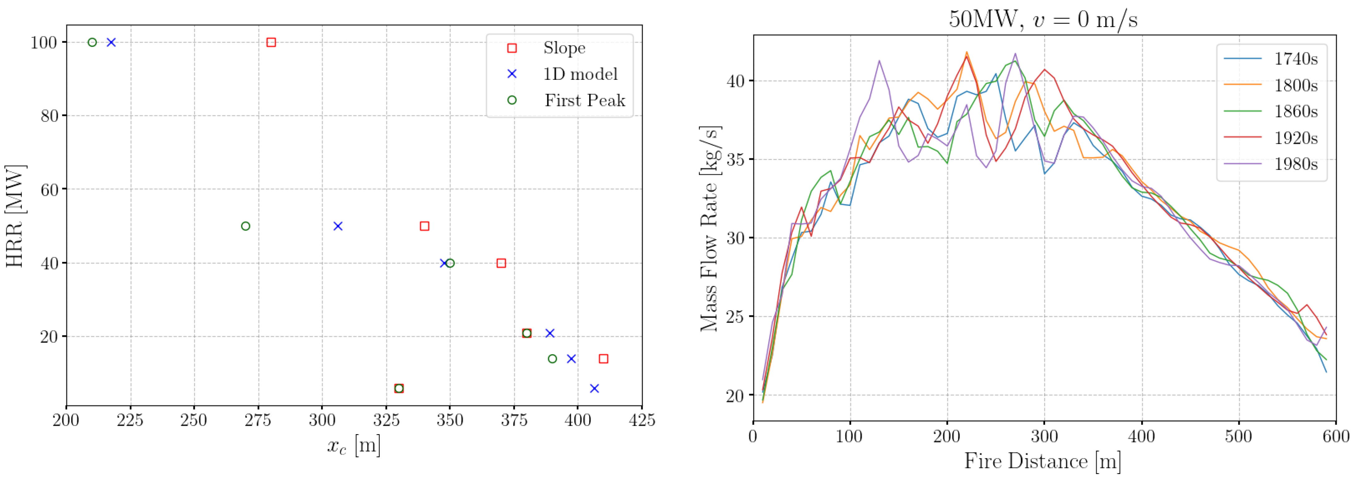
Figure 18 shows the results from both methods without wind. For low HRR, the difference between methods is minimal. At higher HRR, assuming the contamination point occurs at the first peak yields results more consistent with the 1D model, as it accounts for the large vortices in the transition plateau region. In this approach, the first peak is considered an extension of the continuous decrease in the upper layer mass flow rate, which is influenced by vortices. For the 50 MW case, the time selected from CFD simulations to determine the upper layer mass flow rate strongly influences where contamination begins. In this study, the selected time was 1980s. However, when considering the trend across different times, it can be concluded that the contamination point is around 300 m, close to the 306 m predicted by the 1D model.
Figure 18.
The figure on the left shows the results obtained by the two different methods to define the beginning of the contamination of the lower layer, whereas the figure on the right shows the upper layer mass flow rate along the tunnel at different times for 50 MW and, .
For 6 MW, the contamination point from both methods does not match the 1D model prediction. Unlike the other cases, the power is so low that the hot upper layer remains confined within the tunnel, and the model does not account for this particularity.
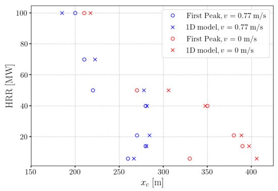
Figure 19 presents a comparison of the results obtained when predicting the contamination point at different HRR levels, with and without wind. Without wind, increasing HRR moves the contamination point closer to the heat source. With wind, this relationship breaks down. The contamination point first moves farther away, then shifts back closer to the heat source at higher HRR. The 70 MW simulation was included to bridge the gap between the 50 MW and 100 MW cases. As HRR increases, wind influences decrease. This occurs because higher HRR levels generate greater velocities inside the tunnel as the local pressure difference induced by the heat source increases. Consequently, the effect of the external pressure difference is reduced at higher HRR, resulting in a behavior that resembles that seen without wind.
Figure 19.
Results obtained for the prediction of the contamination point at different HRR levels, with and without wind.
5. Conclusions
This paper expands upon the work of Galhardo et al. [12] and Ortega et al. [13], primarily by investigating the impact of altering the heat release rate (HRR) on lower layer contamination. A 1200 m horizontal tunnel, with a cross-sectional area of 60 , was simulated using CFD at fire HRRs from 6 MW to 100 MW, both with and without wind. At steady state, increasing HRR did not significantly affect the interface height between layers. However, the 300 soot contour (corresponding to 1.3 m visibility) shifted downward, reaching a minimum height of 1 m in the 100 MW case. It was also noted that, at 6 MW, the velocities generated were so low that the smoke-laden upper layer remained confined within the tunnel. This created a substantially different flow regime than in the other studied cases.
Additionally, a one-dimensional model was developed to predict where lower layer contamination begins. The prediction is based on calculations of upper and lower layer velocities, upper layer temperature, and mass flow rate. In this model, a constant entrainment coefficient is assumed. The results indicated that this coefficient increased with HRR. Furthermore, at lower HRR values, wind tended to reduce the coefficient. Subsequently, it was found that predicting contamination of the lower layer is more accurate when increases with HRR and is obtained from linear regression.
While it is difficult to define exactly where lower layer contamination begins in CFD simulations at high HRR, the 1D model produced consistent results. The main conclusion is that increasing the HRR shifts the contamination point closer to the fire source. Additionally, wind shifts the contamination point upstream, with this effect being more pronounced at lower HRR values.
All information obtained from numerical simulations has been necessary to support the 1D model development. Future work will focus on analyzing smoke contamination in the lower layer across different tunnel cross-sections. In addition, numerical results will be averaged over longer intervals to mitigate the effects of vortices. Once the 1D analytical model is complete, a wide range of numerical simulations will be performed to validate it.
Author Contributions
Conceptualization, J.C.V.; methodology, J.C.V. and P.J.C.; investigation, M.M., U.F. and J.C.V.; writing—original draft preparation, M.M.; writing—review and editing, M.M., U.F., J.C.V. and P.J.C.; supervision, J.C.V. and P.J.C. All authors have read and agreed to the published version of the manuscript.
Funding
This research was funded by Fundação para a Ciência e a Tecnologia (FCT), through IDMEC, under LAETA, project https://doi.org/10.54499/UID/50022/2025.
Data Availability Statement
Dataset available on request from the authors.
Conflicts of Interest
The authors declare no conflict of interest.
Nomenclature
| Latin symbols | |
| A | Cross-section area [m2] |
| c | Proportionality constant [-] |
| Specific heat capacity at constant pressure [J/kg/K] | |
| Hydraulic diameter [m] | |
| f | Friction factor [-] |
| g | Acceleration of gravity [m/s2] |
| Convective heat transfer coefficient [W/m2/K] | |
| Height of the upper layer [m] | |
| Mass flow rate [kg/s] | |
| Prandtl number [-] | |
| Wet perimeter [m] | |
| T | Temperature [K] |
| v | Velocity [m/s] |
| W | Width of the interface between layers [m] |
| x | Longitudinal coordinate [m] |
| Distance from fire to first contamination [m] | |
| Greek symbols | |
| Entrainment coefficient [-] | |
| Slope [%] | |
| Emissivity [-] | |
| Density [kg/m3] | |
| Stefan–Boltzmann constant [W/m2K4] | |
| Maximum difference between layer average velocities [m/s] | |
| Subscripts | |
| e | Entrainment |
| l | Lower layer |
| u | Upper layer |
| w | Wall |
| ∞ | Ambient |
References
- The European Parliament; The Council of the European Union. Directive 2004/54/EC of the European Parliament and of the Council of 29 April 2004 on Minimum Safety Requirements for Tunnels in the Trans-European Road Network. OJ L 2004, 167, 39–91. Available online: https://eur-lex.europa.eu/legal-content/EN/TXT/?uri=CELEX:32004L0054 (accessed on 4 December 2025).
- Hinkley, P. The Flow of Hot Gases Along an Enclosed Shopping Mall: A Tentative Theory; Fire Research Note 807; Fire Research Station: Borehamwood, UK, 1970. [Google Scholar]
- Benjamin, T.B. Gravity currents and related phenomena. J. Fluid Mech. 1968, 31, 209–248. [Google Scholar] [CrossRef] [Scilit]
- Ellison, T.H.; Turner, J.S. Turbulent entrainment in stratified flows. J. Fluid Mech. 1959, 6, 423–448. [Google Scholar] [CrossRef] [Scilit]
- Ingason, H.; Li, Y.Z.; Lönnermark, A. Tunnel Fire Dynamics; Springer: New York, NY, USA, 2015; pp. 1–504. [Google Scholar] [CrossRef] [Scilit]
- Xu, T.; Tang, F.; Xu, X.; He, Q. Impacts of ambient pressure on the stability of smoke layers and maximum smoke temperature under ceiling in ventilated tunnels. Indoor Built Environ. 2023, 32, 85–97. [Google Scholar] [CrossRef] [Scilit]
- Yang, D.; Hu, L.; Huo, R.; Jiang, Y.; Liu, S.; Tang, F. Experimental study on buoyant flow stratification induced by a fire in a horizontal channel. Appl. Therm. Eng. 2010, 30, 872–878. [Google Scholar] [CrossRef] [Scilit]
- Kunsch, J. Critical velocity and range of a fire-gas plume in a ventilated tunnel. Atmos. Environ. 1998, 33, 13–24. [Google Scholar] [CrossRef] [Scilit]
- Tang, F.; He, Q.; Mei, F.; Shi, Q.; Chen, L.; Lu, K. Fire-induced temperature distribution beneath ceiling and air entrainment coefficient characteristics in a tunnel with point extraction system. Int. J. Therm. Sci. 2018, 134, 363–369. [Google Scholar] [CrossRef] [Scilit]
- Jiang, X.; Liu, M.; Wang, J.; Li, K. Study on air entrainment coefficient of one-dimensional horizontal movement stage of tunnel fire smoke in top central exhaust. Tunn. Undergr. Space Technol. 2016, 60, 1–9. [Google Scholar] [CrossRef] [Scilit]
- Caliendo, C.; Russo, I.; Genovese, G. CFD Modeling to Evaluate User Safety by Using Flame Retardants in Asphalt Road Pavements during Large Tunnel Fires. CMES-Comput. Model. Eng. Sci. 2025, 144, 693–715. [Google Scholar] [CrossRef] [Scilit]
- Galhardo, A.; Viegas, J.; Coelho, P.J. The influence of wind on smoke propagation to the lower layer in naturally ventilated tunnels. Tunn. Undergr. Space Technol. 2022, 128, 104632. [Google Scholar] [CrossRef] [Scilit]
- Ortega, E.; Viegas, J.C.; Coelho, P.J. The Contamination of the Lower Layer in Sloped Tunnel Fires. Fire 2023, 6, 245. [Google Scholar] [CrossRef] [Scilit]
- Zhang, X.; Lin, Y.; Shi, C.; Zhang, J. Numerical simulation on the maximum temperature and smoke back-layering length in a tilted tunnel under natural ventilation. Tunn. Undergr. Space Technol. 2021, 107, 103661. [Google Scholar] [CrossRef] [Scilit]
- Yu, L.; Lei, X.; Huang, P.; Liu, C.; Zhang, H.; Yang, F. Study on the combination effect of tunnel slope and longitudinal fire location on the asymmetric flow fields in a naturally ventilated tunnel. Tunn. Undergr. Space Technol. 2024, 146, 105623. [Google Scholar] [CrossRef] [Scilit]
- NFPA 502; Standard for Road Tunnels, Bridges, and Other Limited Access Highways. National Fire Protection Association: Quincy, MA, USA, 2026.
- Caliendo, C.; Genovese, G.; Russo, I. Risk Analysis of Road Tunnels: A Computational Fluid Dynamic Model for Assessing the Effects of Natural Ventilation. Appl. Sci. 2021, 11, 32. [Google Scholar] [CrossRef] [Scilit]
- Caliendo, C.; Genovese, G.; Russo, I. A 3D CFD modeling for assessing the effects of both longitudinal slope and traffic volume on user safety within a naturally ventilated road tunnel in the event of a fire accident. IATSS Res. 2022, 46, 547–558. [Google Scholar] [CrossRef] [Scilit]
- Riess, I. On Smoke Stratification in a 1-D Tunnel Ventilation Model. In Proceedings of the 11th International Conference on Tunnel Safety and Ventilation, Graz, Austria, 9–11 May 2022; pp. 39–46. [Google Scholar] [CrossRef]
- Colella, F.; Rein, G.; Verda, V.; Borchiellini, R. Multiscale modeling of transient flows from fire and ventilation in long tunnels. Comput. Fluids 2011, 51, 16–29. [Google Scholar] [CrossRef] [Scilit]
- OpenCFD Ltd. OpenFOAM (Version 1912). 2019. Available online: https://www.openfoam.com (accessed on 4 December 2025).
- Bechtel; Brinckerhoff, P. Memorial Tunnel Fire Ventilation Test Program. Test Report; Technical Report; Massachusetts Highway Department: Boston, MA, USA, 1995. [Google Scholar]
- Centre d’Études des Tunnels. Dossier Pilote des Tunnels Équipements; Centre d’Études des Tunnels: Bron, France, 2003. [Google Scholar]

Disclaimer/Publisher’s Note: The statements, opinions and data contained in all publications are solely those of the individual author(s) and contributor(s) and not of MDPI and/or the editor(s). MDPI and/or the editor(s) disclaim responsibility for any injury to people or property resulting from any ideas, methods, instructions or products referred to in the content. |
© 2026 by the authors. Licensee MDPI, Basel, Switzerland. This article is an open access article distributed under the terms and conditions of the Creative Commons Attribution (CC BY) license.