Visualization of Hazardous Substance Emission Zones During a Fire at an Industrial Enterprise Using Cellular Automaton Method

Abstract

This article discusses and compares approaches to the visualization of the danger zone formed as a result of spreading toxic substances during a fire at an industrial enterprise, to create predictive models and scenarios for evacuation and environmental protection measures. The purpose of this study is to analyze the features and conditions for the application of algorithms for predicting the spread of a danger zone, based on the Gauss equation and the probabilistic algorithm of a cellular automaton. The research is also aimed at the analysis of the consequences of a fire at an industrial enterprise, taking into account natural and climatic conditions, the development of the area, and the scale of the fire. The subject of this study is the development of software and algorithmic support for the visualization of the danger zone and analysis of the consequences of a fire, which can be confirmed by comparing a computational experiment and actual measurements of toxic substance concentrations. The main research methods include a Gaussian model and probabilistic, frontal, and empirical cellular automation. The results of the study represent the development of algorithms for a cellular automation model for the visual forecasting of a dangerous zone. They are characterized by taking into consideration the rules for filling the dispersion ellipse, as well as determining the effects of interaction with obstacles, which allows for a more accurate mathematical description of the spread of a cloud of toxic combustion products in densely built-up areas. Since the main problems of the cellular automation approach to modeling the dispersion of pollutants are the problems of speed and numerical diffusion, in this article the frontal cellular automation algorithm with a 16-point neighborhood pattern is used, which takes into account the features of the calculation scheme for finding the shortest path. Software and algorithmic support for an integrated system for the visualization and analysis of fire consequences at an industrial enterprise has been developed; the efficiency of the system has been confirmed by computational analysis and actual measurement. It has been shown that the future development of the visualization of dangerous zones during fires is associated with the integration of the Bayesian approach and stochastic forecasting algorithms based on Markov chains into the simulation model of a dangerous zone for the efficient assessment of uncertainties associated with complex atmospheric processes.

1. Introduction

Modern industrial enterprises are characterized by high fire and explosion hazard, with a possible release of toxic substances. Often, a flammable substance is simultaneously a source of toxic hazard; also, when burning, non-toxic materials (complex organic substances, such as petroleum products, fertilizers, plastics, and substances containing heavy metals) emit volatile substances hazardous to humans. These substances are the main components or target products of synthesis, accompanying reagents or intermediate compounds, as well as by-products of various substances’ production [1]. Therefore, the lives of residents of nearby settlements depend on the accurate definition and visualization of hazardous zones for the spread of a cloud of harmful substances during fires at industrial enterprises. The visualization of hazardous zones is necessary not only for planning effective evacuation measures but also for designing industrial enterprises with pre-determined minimum damage to the environment [2], as well as designing residential buildings in industrial clusters.

Also, complex multi-stage technological processes taking place at high temperatures and pressures, as well as with high energy costs, are carried out at chemical industry enterprises. Preconditions are created for the destruction of equipment and the release of large quantities of hazardous substances. Chemical, petrochemical, and other industries process significant volumes of hazardous and explosive substances [3]. Therefore, many chemical enterprises operate in a continuous mode and, consequently, carry an increased potential hazard of environmental impact in the event of the accidental releases of chemical substances [4]. The safety of such enterprises requires the development of effective control systems and means, and the adoption of measures to detect and prevent any deviations in process parameters from the normal operating mode. Such enterprises today are characterized by a high density of technological equipment placement, which contributes to the rapid spread of hazardous substances in the event of a fire or explosion—the occurrence of the so-called “domino effect”—which significantly complicates the localization and elimination of accident consequences [5].

Key issues of the visualization of hazardous zones during fires at industrial enterprises, considered in the works of a number of authors [6,7,8], include the following:

-

Low detection accuracy, which is caused by frequent false alarms of sensors during the field monitoring of the spread of a cloud of toxic gases and the accumulation of a significant number of incorrect data, distorting the results of future modeling;

-

Difficulties in 3D modeling due to significant complication of the system of parameters of hazardous zones when taking into account elevation marks, which complicates navigation for rescuers and leads to errors in assessing smoke zones of different heights;

-

The un-intuitiveness of the interfaces of many software solutions, which makes it difficult for users who are not familiar with the nuances of the physics of the spread of a cloud of combustion products (rescuers, doctors, evacuation organizers, enterprise employees) to make decisions;

-

Difficulties in obtaining operational information from a large number of sensors due to the threat of damage or destruction of modern systems such as LIDAR, drones with gas analyzers, etc. As a result, a fragmented picture of the situation is formed, reducing the accuracy of the visualization of the danger zone.

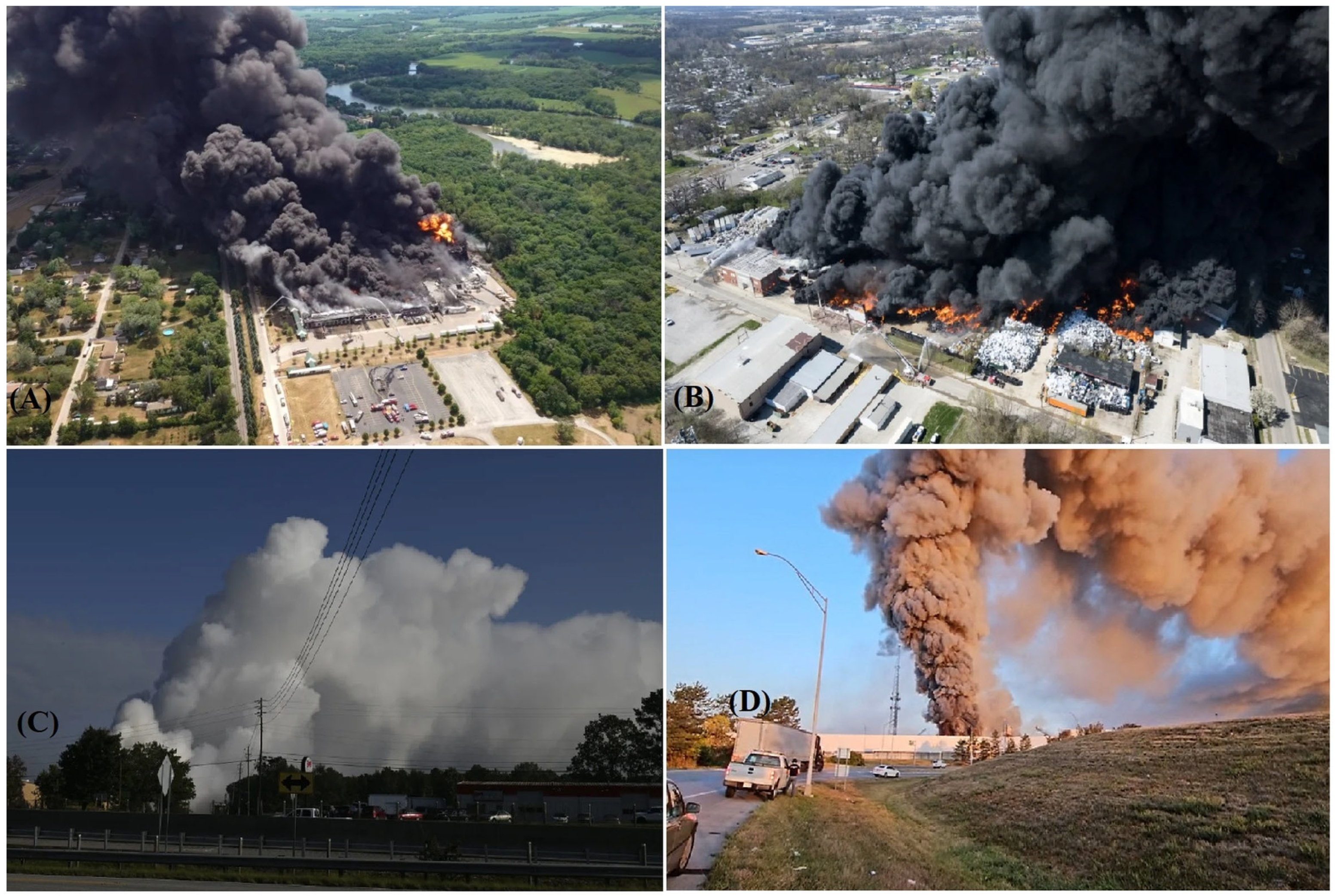
The problem with visualizing the danger zone is the presence of variables that cannot be accurately predicted—the intensity of combustion and emissions of hazardous substances, wind speed, humidity, and atmospheric pressure—while the composition of combustion products and the contours of buildings and structures in the zone of their spread are constant. Therefore, for an accurate visualization of the spread of the danger zone during a fire at an industrial enterprise, simulation modeling using computing power is necessary, since a full-scale fire cannot be experimentally organized or repeated. Computer visualization of the danger zone plays a special role when the enterprise is located near residential areas (Figure 1), which requires special accuracy of simulation modeling.

The purpose of the visualization of the danger zone as the final stage of its simulation modeling is to create a visual mapping of evacuation, rescue, and nature protection measures, the formation of tasks for rescue teams, as well as express damage assessment. Unlike classical mathematical models, the results of the modeling of which reflect the stable behavior of the system over time, the visual representation of the simulation model is subject to experimental errors; therefore, it should be based on the results of appropriate statistical tests. Additionally, the use of a software product that integrates the calculations of the parameters of the danger zone and modules for updating them in real time makes it possible to convey scientifically based visualization results to key participants in the liquidation of the consequences of the accident such as rescuers, firefighters, and persons responsible for evacuation.

The background of the research of pollutant dispersion in the atmosphere begins with the works of G.I. Taylor, who studied heat redistribution in a current over a cold sea at the beginning of the 20th century and conducted the first direct measurements of horizontal turbulent velocity [13]. Later works by F. Pasquill were devoted to atmospheric diffusion [14]. In the second half of the 20th century, the following scientific papers were presented: collections of atmospheric dispersion estimates by D.B. Turner [15] and S.R. Hanna [16]; methods for estimating turbulent diffusion in the environment by G.T. Csanady [17]; in the 21st century, air quality forecasting by P. Zannetti [18].

The basic principles and industry specifics of the simulation modeling of zones of spread of substances hazardous to humans and nature during various accidents at industrial enterprises were developed by T. Drozdova et al. [19], F. Di Giuseppe et al. [20], Huseinov R. [21], and H. Wen et al. [22]. Simulation modeling of hazardous zones during the combustion of substances used in industry was developed by A. Bykov et al. [23], E. Chuvieco et al. [24], A. Tsvirkun et al. [25], C. Sirca et al. [26], etc., including with the help of PC—S. Yemelyanenko et al. [27], Z. Xu et al. [28], etc. The study of the problem of ensuring the safety of workers at industrial enterprises and residents of urbanized areas during fires was conducted by S. Ahmed et al. [29], J. Beringer [30], T.M. Ferreira [31], etc.

Existing studies note the variability of factors influencing the contours of hazardous zones during fires at enterprises, which requires their modeling to include a detailed analysis of the behavior of complex systems, making simulation modeling preferable to “classical” mathematical modeling. Therefore, the visualization of hazardous zones requires significant time expenditures to optimize the parameters of combustion processes and the spread of its harmful products. Therefore, it should be taken into account that despite the impossibility of obtaining a complete picture of the spread of a hazardous zone when visualizing it [32], the results of this process are quite sufficient for the proactive planning of measures to evacuate people and take environmental protection actions.

According to the experts [33], many methods and algorithms for automated calculation of the consequences of a hazardous substance release are intended for qualified users and have limitations associated with the idealized nature of the description of the diffusion and transfer processes of chemical substances. Such features and limitations can negatively affect the adequacy and efficiency of the response, especially in the case of a deficit or uncertainty of the initial information. Extreme decision-making conditions arising as a result of an emergency dictate requirements for the mobility, autonomy, and speed of the forecasting and visualization system, which will allow, based on monitoring data, for the calculation and displaying of the contamination zone on a map of the area. One of the promising areas for developing algorithms for such a system is a cellular automation approach to modeling gas dynamics, which allows for taking into account the effects of the dispersion of a pollutant cloud during a local scale of an accident.

2. Materials and Methods

The process of emergency development at an industrial enterprise is usually considered in the form of three interconnected phases, each of which is characterized by specific features and scales of negative consequences [34].

The first phase of an emergency (phase A) is limited to the process unit or workshop. At this stage, local breaches of equipment tightness or minor fires in the equipment may occur. There is no threat of the accident spreading beyond the isolated section of the enterprise, and the personnel respond according to the instructions.

The second phase, characterized by a high risk of fire spreading through the workshop or process unit (phase B), creates conditions for chain fire development with the probability of involving the entire enterprise in the emergency process. Therefore, the forces and means of response of the enterprise itself are involved in localizing the consequences of the fire. However, at this stage, the occurrence of a full-scale pollution spot is characterized by a low probability.

The critical phase of fire development (phase C) is the most dangerous stage of emergency situation development, characterized by chain spread of fire beyond individual workshops or warehouses, and the ignition of most of the sources of hazardous substances. All available forces and means of response of the enterprise, as well as local fire services, are involved in eliminating the consequences of a fire of such scale. For such a scenario, the predictive and actual visualization of the zone of spread of hazardous substances is of particular importance, with the definition of the boundaries of emissions and spread of hazardous substances, taking into account obstacles to the movement of polluted air masses in the form of tall buildings and structures and forest plantations. The success of evacuation measures, including the declaration of an emergency regime, depends on the completeness of the definition of points forming the boundary lines of the hazardous zone, taking into account all the variable parameters of emissions of hazardous combustion products. In turn, the accuracy of visualization depends on the applied simulation methods.

The most critical cases are non-design basis accidents, for which a prompt response requires estimated information on the boundaries of hazardous substance emissions, the size of the hazardous pollution zone, and the facts of its exit beyond the sanitary protection zone of the enterprise, since the adequacy of the decisions made depends on its analysis. Such information can be obtained on the basis of processing chemical reconnaissance data in the system for predicting the consequences of emergency emissions, which allows for displaying zones of possible chemical pollution on a terrain map.

Existing studies of fire hazard area identification use Bayesian inference to estimate the probability distribution of emission parameters based on field observations [35]. Sampling methods such as Markov Chain Monte Carlo or Sequential Monte Carlo [36] are used to find the posterior distribution. The computation time in this case can increase significantly, which is one of the disadvantages of probabilistic methods. Geostatistical methods allow for predicting the values of variables at unknown points based on measured data at known points [37]. Deterministic spatial interpolation methods include nearest neighbor, linear interpolation, Delaunay triangulation [38], Voronoi Diagrams [39], and inverse distance due to their simplicity and computational efficiency. To estimate the chemical contamination zone, the kriging method can be applied [40], which is used to predict the values of a random field based on observations at other locations. The clearing results are presented as a variogram, which displays the variation between pairs of measurements depending on the distance between them.

The Bayesian approach to estimating uncertainties associated with the description of complex atmospheric processes operates with both a priori data and field observations. This approach updates a priori assumptions about the parameters of the pollution distribution taking into account the observed data. The likelihood function is used to assess the agreement between the measured and predicted observations. Information about the parameters and their uncertainty is extracted from the posterior statistics, which are characterized by the mean and standard deviation of the values.

To solve the problem of the “curse of dimensionality”, various sampling algorithms are used, such as Markov Chain Monte Carlo (MCMC), which evolves to the posterior distribution [41]. Many algorithms have been proposed to generate new states of the Markov Chain and determine their acceptability; for example, the Metropolis–Hastings algorithm [42].

A common problem in the statistical analysis of fire hazard zone boundary data at an enterprise is the problem of data shortage, which affects the reliability and validity of visualization. Reducing the volume of measurements increases the sensitivity of the algorithm to random noise and data outliers, which can lead to incorrect conclusions and errors in parameter estimation [43]. At the same time, Bayesian methods have an advantage in displaying source estimates with appropriate levels of reliability, but require increased computational resources, which is especially important when using complex algorithms of computer hydroaerodynamics.

The main advantage of the neural network approach is the ability to approximate complex nonlinear functions in the problem of inverse modeling of the distribution zone of hazardous substances, which contains many variables and potentially nonlinear interactions [44]. However, there are a number of problems that limit the possibilities of practical application of neural network algorithms—existing “gaps” in the theoretical justification of network algorithms, as well as problems of network training on available data. With a small training sample, the network algorithm can “overtrain” and incorrectly generalize new data. In inverse modeling problems, such an algorithm is effective only for the accident variants on the actual data of which it was trained. Unlike other algorithms, such as “decision trees”, neural network algorithms are actually “black boxes”. The lack of interpretability of such algorithms can negatively affect the situational analysis of an accident. The use of neural networks and other machine learning algorithms requires large amounts of data for training and validation of models, which is problematic under conditions of limited or no actual data for the operational construction of a fire hazard zone model and its visualization. Under these conditions, it is advisable to use synthetic data from forecast models.

The existing cellular automation approach [45,46] is one of the most effective approaches to the development of such algorithms. In this approach, the entire spatiotemporal emission region is presented as an array of cells of the computational grid, and each cell of such a region can be in one of several states. Cellular automation algorithms are based on the concept of locality [47]. A cell is updated based on the states of nearby cells in accordance with a set of decision rules. These rules are simple and constant in time, but can vary in space. When a cellular automation functions, a synergistic effect is manifested, which is not typical for the behavior of an individual particle. Such algorithms can be used to predict various processes during ignition, fire spread, and clouds of hazardous combustion products, including physical, chemical, and biological ones, which makes this approach convenient for visualizing the danger zone. At the same time, the cellular automation does not take into account complex chemical reactions or meteorological effects without additional modification or supplementation with other models [48].

The first step in visualizing a dangerous zone during a fire at an industrial enterprise is a mathematical description of the formation and spread of toxic combustion products in the atmosphere—a real system—using the characteristics of the main events. The model of the formation of a dangerous zone of combustion product spread is adopted in the form of a mathematical and geometric model, as well as an algorithm for processing information adopted in a specific statistical method. The main factors in the process of the formation and spread of a dangerous zone are the mass of combustion products, as well as the speed of spread of a cloud of harmful substances in the atmosphere, taking into account the wind direction [49].

2.1. Development of a Method for Modeling the Release of Hazardous Substances During a Fire at an Industrial Enterprise

The scheme for selecting forecasting algorithms developed by the authors is presented in Figure 2. The input data for the selection are reference measurements of the concentration of hazardous substances in the atmosphere and the requirements for the forecast.

The choice of a specific algorithm depends on the scale of the consequences of the emergency release, the requirements for the speed of calculation and the informativeness of the forecast, as well as the possibility of taking into account specific dispersion factors:

-

The algorithm based on the Gauss equation is used to forecast the operational situation at the meso-scale level of the accident;

-

The empirical cellular automata algorithm is used for express assessment of the operational situation at the local scale of the fire;

-

The probabilistic cellular automata algorithm is selected to obtain more informative and stable forecasts at the local scale of the fire;

-

The frontal cellular automata algorithm is used to form an intermediate version of the forecast at the local scale of the fire.

2.2. Using the STE Method

Source term estimation (STE) methods provide the calculation of hazard zone parameters based on monitoring data. The inverse modeling procedure used in STE algorithms [50] is associated with the processing of noisy and sparse input data (due to unstable atmospheric conditions and sensor “noise”). Some STE algorithms are based on the adjoint source–receptor relationship approach [51], where sensors are represented as emission sources and the wind direction is inverted. It should be recognized that STE algorithms provide high performance in scenarios with little or no noise, simple flat environments, a large number of sensors and a single source; however, in real scenarios, these conditions are not met. In particular, built-up areas lead to a recirculation zone of the polluted airflow field and splitting of the combustion plume around buildings and structures.

The problem of dispersion in the accumulation medium has been addressed previously using computational fluid dynamics (CFD), which is only accurate enough over a certain distance [52].

For such phenomena, the most accurate solution is computational fluid dynamics (CFD)-based forecasting.

In particular, A. Keats et al. demonstrated the performance of a CFD-based “STE solver” in an urban setting [53] using the Joint Urban 2003 experiment data set [54]. P. Kumar et al. [55] successfully used STE algorithms to predict emissions in an urban setting based on the Mock Urban Setting Test [56]. However, such solutions are computationally expensive [57].

According to the works of B. Widrow and S.D. Stearns, the problem of adapting a complex system, to which a system with an “STE solver” can be attributed, is reduced to the problem of finding the extreme value of some objective function under conditions of insufficient a priori information [58]. It is also noted that such systems for estimating unknown emissions in the atmosphere consist of three components [59]:

• The first component is a network of receptors (sensors) for detecting hazardous substances, measuring their concentrations at different points.
• The second component is an atmospheric dispersion model for predicting concentrations of hazardous substances in space and time.
• The third component is integration algorithms for combining measured concentrations with atmospheric dispersion models to determine the parameters of unknown emissions.

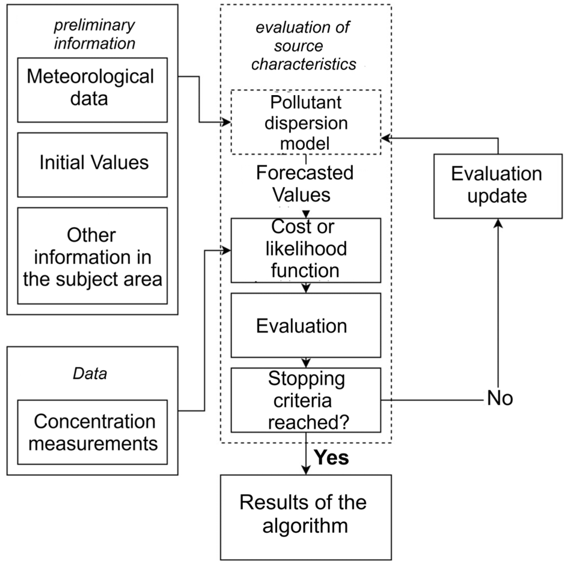
These components allow for estimating the characteristics of the source of hazardous substance emissions into the atmosphere during a fire based on a limited set of concentration measurements. In the system with the “STE solver” predictive estimates of the location coordinates, intensity of hazardous substance emissions and other parameters of modeling the hazardous zone during a fire are formed. The information-processing scheme in the STE approach (Figure 3) contains internal and external information-processing loops [50].

A number of studies have been devoted to the issues of collecting and processing information in the external loop of the system. Thus, when selecting algorithms for the internal loop, classical models of impurity dispersion are usually used. In the works of T.O. Spicer and J. A. Havens, a comparison of Gaussian models and heavy gas models is given [60]. Approaches to the formation of the objective function in the validation of impurity dispersion models are reflected in the works of S.R. Hanna and J. Chang [61]. The issues of convolution of the multi-objective function are also described in detail in the studies of D. Thevenin at al. [62].

The sliding window method [63] allows one to generalize field observation data and form a reference sample for constructing a dynamic forecast model. The window size corresponds to a predetermined time interval for information processing. When selecting the size of the sliding window, the possibility of processing data in real time is taken into account. A large window size leads to forecast errors for rapidly changing conditions. There are gaps in values and outliers in the array of accumulated information. In such cases, analytical algorithms for data recovery are used in practice with subsequent assessment of the reliability of the results.

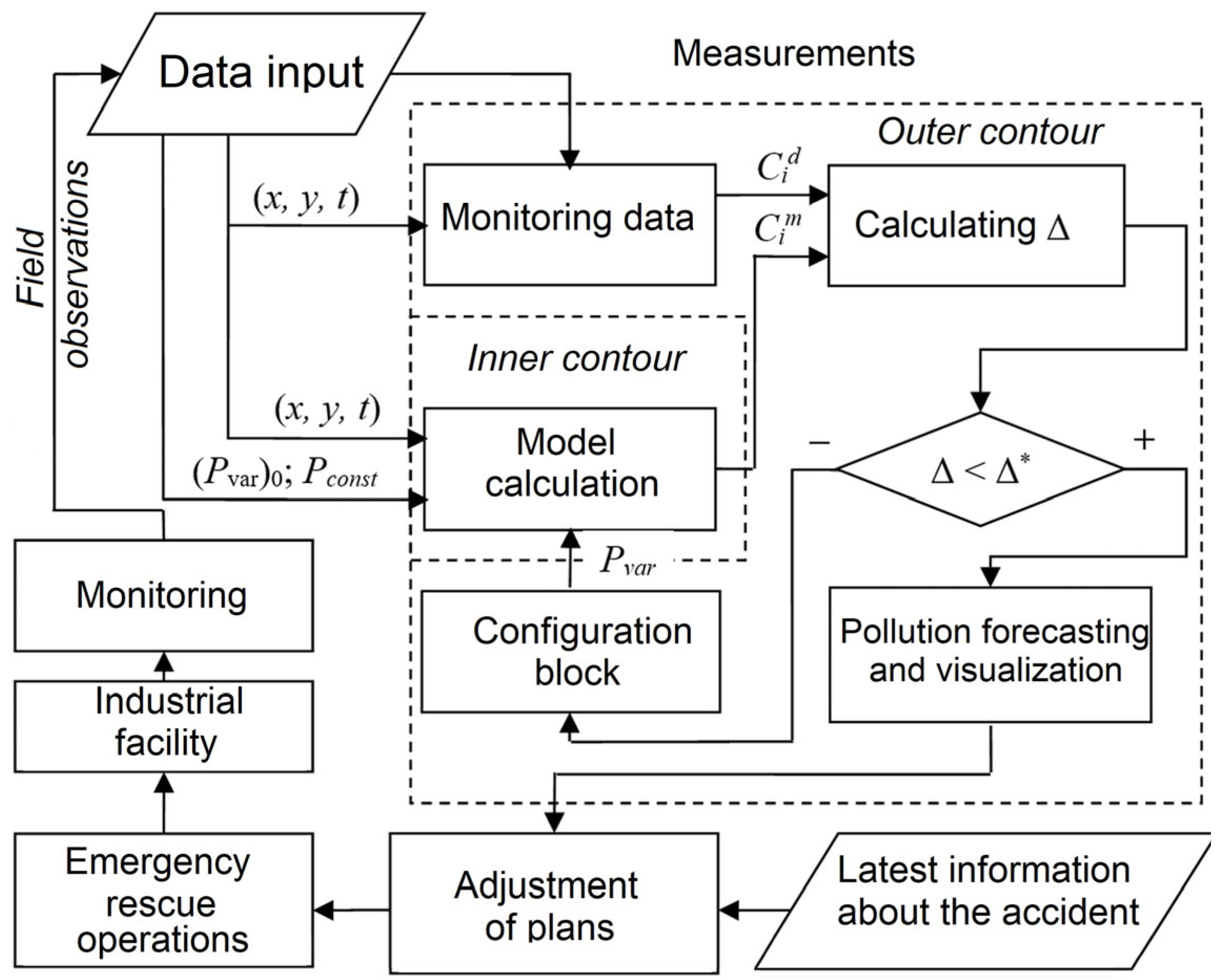
The presented STE approach is chosen as a basis for developing the method, as well as the algorithms for forecasting and visualizing the hazardous pollution zone, combined into a single scheme (Figure 4) of two-loop information processing. In the inner loop of such a scheme, the forecast result is formed; in the outer loop, the parameters of the forecast model are calculated based on the chemical reconnaissance data of the area. The problem of finding the forecast parameters is presented as follows: based on the monitoring data C_i^d(x,y,z,t) and the a priori specified parameters P_const of the assessment of the operational situation, the values of the variable parameters P_var of the forecast C_i^m(x,y,z,t) are determined, which provide a minimum of the objective Function (1) under the constraints (P_var)_lower ≤ P_var ≤ (P_var)_upper:

∆ = F(C_i^m(x,y,z,t), C_i^d(x,y,z,t)) → min,

(1)

where F(*,*) is the criterial assessment of the forecast, is the number of the observation–forecast pair, $i=\overline{1,M}$ is the number of pairs, and the indices “lower” and “upper” denote the lower and upper limits of the parameter changes. The definition of min ∆ is the basis for visualizing and analyzing the hazardous pollution in the area (∆* is the measured value).

The basis [32] for implementing this method is the generalized emergency situation processing scheme, which is shown in Figure 4.

The processing scheme covers the procedures for monitoring the state of the object and predictive modeling. At the monitoring stage, after the topological binding of the observation sensors, a set of measures is carried out related to the calculation of the sensor polling period and the resolution of issues related to the organization of the software and hardware interface between the sensors and the visualization system platform. If such an interface is absent, then the concentrations of hazardous substances at the observation sites and the coordinates of the sensor location (x, y, z) are entered into the system manually. At the modeling stage, a priori data on the accident are used to calculate the forecast parameters, which serve as the basis for constructing concentration fields and calculating the area of hazardous contamination. The search for the best parameters is based on solving the problem of minimizing the deviation ∆ from the tolerance ∆f on a set of possible forecast parameters P_var.

The research area is limited by variants of turbulent, passive emissions into the atmosphere at micro- and meso-level scales of accidents. Examples of long-term emissions of hazardous chemical substances are considered for the case of a stationary location of the pollution source. In the report [64], three scales of representation of the atmospheric flow are analyzed: the micro-scale (<1 km) describes a complex flow depending on the characteristics of the surface; at the meso-scale (1–1000 km), the flow takes into account hydrodynamic effects and heterogeneities of the energy balance; at the macro-scale (>1000 km), the flow is associated with synoptic phenomena and the distribution of baric systems.

Under the conditions of a rapid response to an emergency situation, it is often not possible to justify the exact layout of the sensors. However, as shown in [32], the most significant are observations and measurements performed directly on the emission axis. The possibilities of rapid response to emissions of hazardous substances determined the requirements for the maximum visualization radius, the value of which was 10 km (micro- and meso-scale levels). With such a radius, there are opportunities for collecting, processing, and transmitting monitoring data, including via wireless communication channels. New LPWAN (Low-Power Wide Area Network) technologies cover areas at a distance of up to 10 km with minimal energy consumption and are capable of ensuring the functioning of monitoring systems with remote sensors [65].

In the study presented below, a turbulent gas flow regime was reproduced. Turbulence is the most common type of continuous media motion and is present in many phenomena [66]. With increasing distance from the emission source, the influence of effects caused by gravitational dispersion gradually weakens. Atmospheric turbulence, caused by wind currents, convection, and surface roughness, becomes the dominant force in the process of pollutant propagation. At large distances from the source, the emission is diluted, and its density approaches that of air.

When predicting the consequences of an accident in an operational environment, it is often necessary to simplify calculations [67]. The implementation of complex dispersion algorithms that take into account the reactivity of a substance leads to significant time costs for calculating the consequences of a release and reduces the effectiveness of emergency response measures. If the released substance does not affect the atmospheric flow [68], then it is considered “passive” and is dispersed by the surrounding flow. Therefore, calculations of the atmospheric flow and dispersion of pollutants can be separated, which allows for using different types of algorithms for each of these processes. Thus, to calculate a pollution map, data from a meteorological model are required, as well as the results of the impurity dispersion forecast.

When developing the integrated system, the features of choosing a forecasting algorithm depending on the properties of the pollutant were taken into account. For example, in the ALOHA 5.4.7 (Areal Locations of Hazardous Atmospheres) software, the DEGADIS 2.1 (Dense Gas Dispersion) algorithm for dense (heavy) gas dispersion [69] is usually selected to reproduce the effects of chlorine emission. It is used to assess the short-term concentration of hazardous substances in the environment and analyze the expected area of pollution when the threshold values of such concentration are exceeded. It is relevant in cases of the emission of dense gaseous pollutants (heavier than air), when the measurement data exceed dangerous concentration levels. During transfer and dispersion, the content of the impurity in the emission cloud gradually decreases and the emission becomes “less dense”. Therefore, upon reaching a certain emission density, the transition to the Gaussian algorithm is implemented in this system.

To predict the consequences of an emission at a meso-scale accident in the internal circuit of the system, the work proposes to use the Gauss algorithm, and at a local scale of an accident (microscale up to 1 km), cellular automation algorithms.

Among the internal circuit algorithms, stationary model algorithms are widespread, in which only the spatial distribution of the impurity is calculated [50]. The low complexity of such algorithms significantly simplifies the modeling procedure, increases the speed of calculations, and reduces the requirements for the implementation of algorithmic support.

2.3. Using Gaussian Models

Stationary Gaussian models have the advantages of being well studied, taking into account factors that influence the process of spreading hazardous substances (e.g., wind speed and atmospheric stability) and do not require significant computational resources. At pollution scales over 1 km, the effects of obstacles do not affect the extent to which the contamination pattern changes at a local scale of an accident [64].

The above features determine the possibilities of choosing algorithms of the Gauss model for forecasting the consequences of an accident, but they are developed for ideal emission conditions—stationary and uniform flows of hazardous substances, normal distribution of the concentration field, which does not always correspond to the real situation. The Gauss approach is also characterized by other limitations, such as low efficiency in weak and variable winds and insufficient accuracy under difficult conditions of impurity dispersion.

At a local scale of an accident, specific dispersion factors prevail [64], which include the configuration of field flows and obstacles. In this case, it is advisable to use numerical model algorithms to predict and visualize the processes of occurrence and development of emergency situations. There are a large number of such models that can be assessed by resource costs, speed, and accuracy of predictions, and these criteria are closely related to each other. As noted earlier, at a local scale of an accident under the conditions of development of the area, high-speed cellular automation algorithms were used in the work to predict emissions of hazardous substances.

The best-known Gauss equation [70] can be used to calculate the area in the contours of the spread of a cloud of hazardous substances. With a continuous point emission of combustion products and a constant wind speed, it can be represented in the following Formula (2):

$$\begin{array}{l}C(x,y,z,p,\mathrm{z}0)={\displaystyle \frac{Q^{*}}{2\pi {\sigma }_y(x,p,z0){\sigma }_z(x,z0)U}}\cdot \exp \left[-{\displaystyle \frac{{\left(y-y_0\right)}^2}{2{\sigma }_y^2(x,p,z0)}}\right]\\ \left[\exp \left(-{\displaystyle \frac{{(z-h)}^2}{2{\sigma }_z^2(x,z0)}}\right)+\exp \left(-{\displaystyle \frac{{(z+h)}^2}{2{\sigma }_z^2(x,z0)}}\right)\right]\end{array}$$

(2)

where C(x,y,z,p,z0)—concentration of hazardous substances in the atmosphere, g/m³;

Q—emission intensity, g/s;

y₀—emission source coordinate, x, y, z—concentration measurement coordinates;

U—average wind speed, m/s;

h—height of hazardous substance source in the atmosphere, m;

p—atmosphere stability category;

z0—roughness coefficient;

σ_z and σ_y—vertical and horizontal dispersion parameters; the value Q* = Qf_Ff_W takes into account cloud depletion corrections; f_F and f_W—dry and wet impurity deposition coefficients.

From Equation (1) it follows that the concentration of the impurity C(x,y,z,p,z0) depends significantly on the parameters of the vertical σ_z and horizontal σ_y dispersion, the methods of estimating which take into account the classification of weather conditions and the characteristics of the underlying surface.

To calculate the parameters of the vertical σ_z and horizontal σ_y dispersion of the impurity stream, the Smith–Hosker dispersion curves and Briggs formulas [71], which are common in engineering practice, were used in the work.

The Smith–Hosker dispersion curves are defined by Formulas (3)–(5):

$${\sigma }_z(x)=\left\{\begin{array}{c}F(z0,x)\cdot g(x) \mathrm{if} F(z0,x)<{\sigma }_z^{\max }(x)\\ {\sigma }_z^{\max }(x) \mathrm{if} F(z0,x)\ge {\sigma }_z^{\max }(x)\end{array}\right.$$

(3)

$$F(z0,x)=\left\{\begin{array}{c}\ln [c_1\cdot x^{d_1}\cdot (1+{(c_2\cdot x^{d_2})}^{-1})], \mathrm{at} z0>0.1 \mathrm{m}\\ \ln [c_1\cdot x^{d_1}\cdot {(1+c_2\cdot x^{d_2})}^{-1}], \mathrm{at} z0\le 0.1 \mathrm{m}\end{array}\right.$$

(4)

$$g(x)={\displaystyle \frac{a_1\cdot x^{b_1}}{1+a_2\cdot x^{b_2}}}$$

(5)

In Equations (2)–(4) the following are specified in a tabular manner: the dependencies of the parameters a1, a₁, a₂, b₁, and b₂ on the atmospheric stability category p; the dependencies of the parameters c₁, d₁, c₂, and d₂ on the roughness coefficient z0; the values of the upper limit σ_z^max(x) for different atmospheric stability categories. The piecewise quadratic interpolation method of tabular data can be used to determine the specified parameters. Briggs’ formulas are represented by Equations (6)–(9):

$${\sigma }_y(x)={\displaystyle \frac{c_3(p,z0)\cdot x}{\sqrt{1+c_4(z0)\cdot {10}^{-4}\cdot x}}}$$

(6)

$$c_3={10}^{a(p)+3.8\cdot {10}^{-2}{(\lg z_0+2.816)}^2}$$

(7)

$$c_4={(10\cdot z0)}^{0.21+0.13\cdot \lg (10\cdot z0)}$$

(8)

$$a\left(p\right)=7.536\cdot {10}^{-3}\cdot p^2-0.1757\cdot p-0.7$$

(9)

where p is the parameter of atmospheric stability.

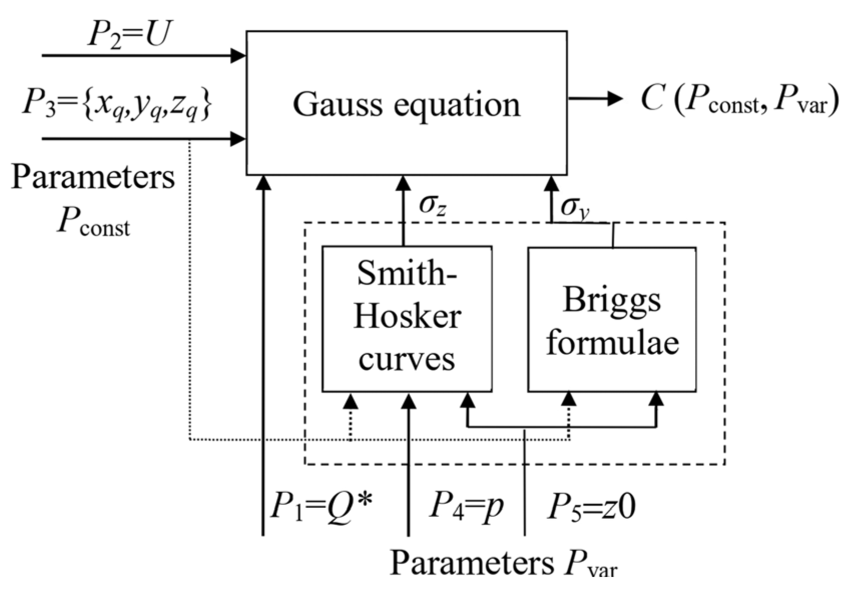
The variable parameters of the forecast based on the Gauss Equation (1) include the emission value Q*, the roughness coefficient z₀, and the atmospheric stability parameter p. Figure 5 shows the developed scheme for calculating the concentration of hazardous substances with constant and variable forecast parameters.

The forecast parameters P_const include the following: P₂ = U—average wind speed along the emission axis, m/s; P₃ = {x_q,y_q,z_q}—coordinates of the emission source q, as well as the variable parameters P_var; P1 = Q*—amount of hazardous chemical emissions, g/s; P₄ = p—atmospheric stability; P₅ = z₀—surface roughness coefficient.

Along with the advantages of such methods of modeling the concentration of hazardous substances in the atmosphere as STE and integral models, one cannot fail to note the insufficient accuracy of their prediction of the contours of the cloud of combustion products.

2.4. Using Cellular Automation Approach

The cellular automation approach [45] to modeling gas dynamics, based on empirical assumptions, simple algorithms, and decision rules, is capable of not only qualitatively describing the spatiotemporal form of the emission but also quantitatively assessing its statistical characteristics. In particular, Toffoli models of asynchronous naive diffusion and block-synchronous diffusion with Margolus vicinity [46] are important for us.

In addition, the algorithm of the cellular diffusion model with von Neumann neighborhood is effective under the following assumptions [72]:

• A flat case of representing the emission region as an array of cells of a regular two-dimensional grid, the horizontal dimensions of which correspond to the scale of data display on the map. The concentration of the impurity in the neighborhood of the cell has a value averaged with respect to the height z, which can be used to estimate the concentration isopleths.
• An integrated approach to the problem of modeling the processes accompanying the emission (emission processes, wind mass transfer, diffusion and sedimentation) and requiring consideration of many factors associated with the meteorological state of the atmosphere, the conditions of emission, and the dispersion of the impurity in the adjacent area.
• The probabilistic nature of the cellular automation model, due to the uniqueness and specificity of the conditions of the emission of toxic substances. The distribution functions of the parameters are random, with probabilistic properties unknown in advance. Under the hypothesis of the normality of the distribution law of functions, it is possible to calculate concentration isopleths based on measurement data, as well as an interval estimate of the area of the contamination zone with a confidence probability specified by the “three sigma rule” [73].

Assumptions adopted:

(A)

The emission area is presented as an array of cells of a two-dimensional grid.

(B)

An integrated approach is used, taking into account the complex conditions of emission and dispersion of the impurity in the adjacent area.

(C)

Based on the probabilistic properties of the emission parameter distribution.

(D)

The impurity cloud is modeled as an ensemble of test particles settling in the surface cells, taking into account the rules for avoiding obstacles.

The scheme for calculating the concentration of a pollutant based on the probabilistic cellular automation is shown in Figure 6. The main parameters of the cellular automation model: P = {m*, σ*, B, K, Q*, U*, x₀, y₀}, where m* is the mathematical expectation of the wind direction; σ* is the standard deviation of the polar angle; B is the array of obstacles; K is the coefficient of building density; Q* is the emission intensity; U* is the wind speed (m/s); x₀, y₀ are the source coordinates; Y is the pollutant concentration field. The entire emission area is represented as a set Ω of square-shaped surface cells of equal area, the structure of which is divided into the following components: Ω1 is the internal cells of the environment; Ω2 is the boundary cells; Ω3 is the source cells; Ω4 is the obstacle cells; Ω5 is the cells of the presence of an impurity, Ω6 is the cells of the measurements taken.

The algorithm of probabilistic cellular automation with von Neumann neighborhood is developed on the basis of statistical testing method (Monte Carlo), in which the cloud of impurity is modeled as an ensemble of test particles settling in surface cells taking into account the rules of obstacle avoidance. The algorithm with imitation of particle flight contains procedures of initialization, generation and transfer of particle, formation of concentration map (Figure 6).

The asynchronous mode of operation of the cellular automation is based on the transition rule in the cycle “particle generation—area filling”, sequentially applied to the source cell x ∈ Ω₃. After the particle generation, the transition rules in the template T(x) are specified by the probabilistic contextual substitution Θ_k(x), and the conditions for filling the area are formed by the spatial contextual substitution Θ_q(x). Thus, the transition function Ψ₁: P × V → V is represented by the system of substitutions Ψ₁(x) = Φ(Θ_k(x), Θ_q(x)) and has the following Formulas (10)–(12):

$${\psi }_1:\left\{v_0\left(i,j\right),v_1\left(i,j+1\right),v_2\left(i+1,j\right),v_3\left(i,j-1\right),v_4\left(i-1,j\right)\right\}· \left\{\left(v_k,x\right),\left(\left(v,x_q\right)\right)\right\}\to \left\{v_k\left(i_q.j_q\right)\right\}$$

(10)

$${\Theta }_k:\left(v_0,x\right)\to \left(v_k,x\right), k=\left\{\begin{array}{c}1, if 0<{rand}_{nd}\le 0.25\\ 2, if 0.25<{rand}_{nd}\le 0.5\\ {\displaystyle \genfrac{}{}{0pt}{}{ 3, if 0.5<{rand}_{nd}\le 0.75}{4, if 0.75<{rand}_{nd}\le 1}}\end{array}\right.$$

(11)

$${\Theta }_q:\left(v_k,x\right)\to \left(v,x_q\right), v=\left\{\begin{array}{c}0,\left(i_q,j_q\right)\in M_1\\ 1,\left(i_q,j_q\right)\in M_2\end{array}\right.$$

(12)

where rand_nd(m*, σ*) is a random number of the normal distribution law, defining the angular direction of the particle’s flight with the estimated mathematical expectation m* = m/360° + 0.125 and the standard deviation σ* = σ/360°.

An accurate visualization of the danger zone requires calculating the particle’s trajectory taking into account obstacles. The order relation in the ordered set L_path is defined by the rules of the particle’s flight with the address x ∈ L_path in the T_x neighborhood of neighboring cells:

-

There is a path L_path consisting of cell addresses X, which represent a sequence of “steps” of the particle.

-

The order relation on the elements of the path L_path is based on the order of the “steps” of the particle. The next step is determined as follows: Each subsequent element (L_path)_i+1 of path L is formed based on the rules of the particle’s flight in the T_x neighborhood of cells corresponding to the current element (L_path)_i.

-

The order of elements in the path L_path can be established based on the increasing order of the “steps” of the particle.

Within the framework of the cellular automation approach, the basic rules for the movement of a particle with the formation of contours of a dangerous zone for the spread of combustion products during a fire at an industrial enterprise include the following:

• The neighboring cell is free and belongs to the set of internal cells of the environment x ∈ Ω₁. The procedure for forming the path L_path is completed by filling the final cell.
• The neighboring cell belongs to the set of cells of the presence of impurity x ∈ Ω₅. The procedure for forming the path L_path is resumed.
• The neighboring cell belongs to the obstacle region x ∈ Ω₄, forbidden for the cell to pass. The new direction of the path L_path is corrected.
• The neighboring cell belongs to the boundaries of x ∈ Ω₄, restricting the movement of particles. The particle completes its path and is destroyed.
• The particle was previously in a neighboring cell. Corrections are introduced into the new direction of the path L_path.

The given rules are caused by the effects of interaction with obstacles, problems of particles “hanging” in voids, as well as significant time costs when the directions of flight are scattered or particles move against the wind. It should be noted that some of these problems could be resolved by using meteorological model data.

The following are introduced into the particle trajectory calculation scheme: an array of particle names L_pn and an integer array L_pv, which records the number of visits of a wandering particle to the current cell. A record of the particle’s path is formed, which is necessary for monitoring repeated visits to a neighboring cell.

If an obstacle appears on the particle’s path (or the cell has the maximum number of passes among other neighbors), then it drops out of the candidates. If the cells within the template T have the same number of passes, then the priority is set in accordance with the minimum deviation ∆L between the random variable θ_xn, and the direction to the center of the candidate cell (13):

$${∆}_L=\mathrm{m}\mathrm{i}\mathrm{n}\left(\left|t_k-0.5\right|,\left|t_k-4.5\right|,\left|t_k+3.5\right|\right)$$

(13)

where t_k = Θ_xn – k; the value k corresponds to the contextual substitution Θ_k(x).

When selecting the next step of the path L_path, the priority is given to the number of particle entries into neighboring cells. Thus, the rules for moving a particle are the basis for calculating the path of a “settled” particle.

The configuration of the contamination spot during the frontal expansion of the emission area characterizes only the fact of the presence or absence of an impurity in the emission area under study; therefore, to obtain the concentration, information about the number of the “settled” particle is used, which is accumulated in the statistics array R.

One of the approaches to modeling phenomena with a large number of unknowns is the Monte Carlo method. Carrying out a series of experiments and averaging the results R allows for increasing the stability of the results of probabilistic modeling.

Based on the results of a series of experiments, the averaged distance field S_x (14) is calculated:

$$S_x={\displaystyle \frac{\sum _{i_{exp}=1}^{N_{exp}}{R}_{{x,i}_{exp}}}{N_{exp}}}$$

(14)

where i_exp is the experiment number; N_exp is the dimension of the series of experiments

2.5. Obtaining a Concentration Map

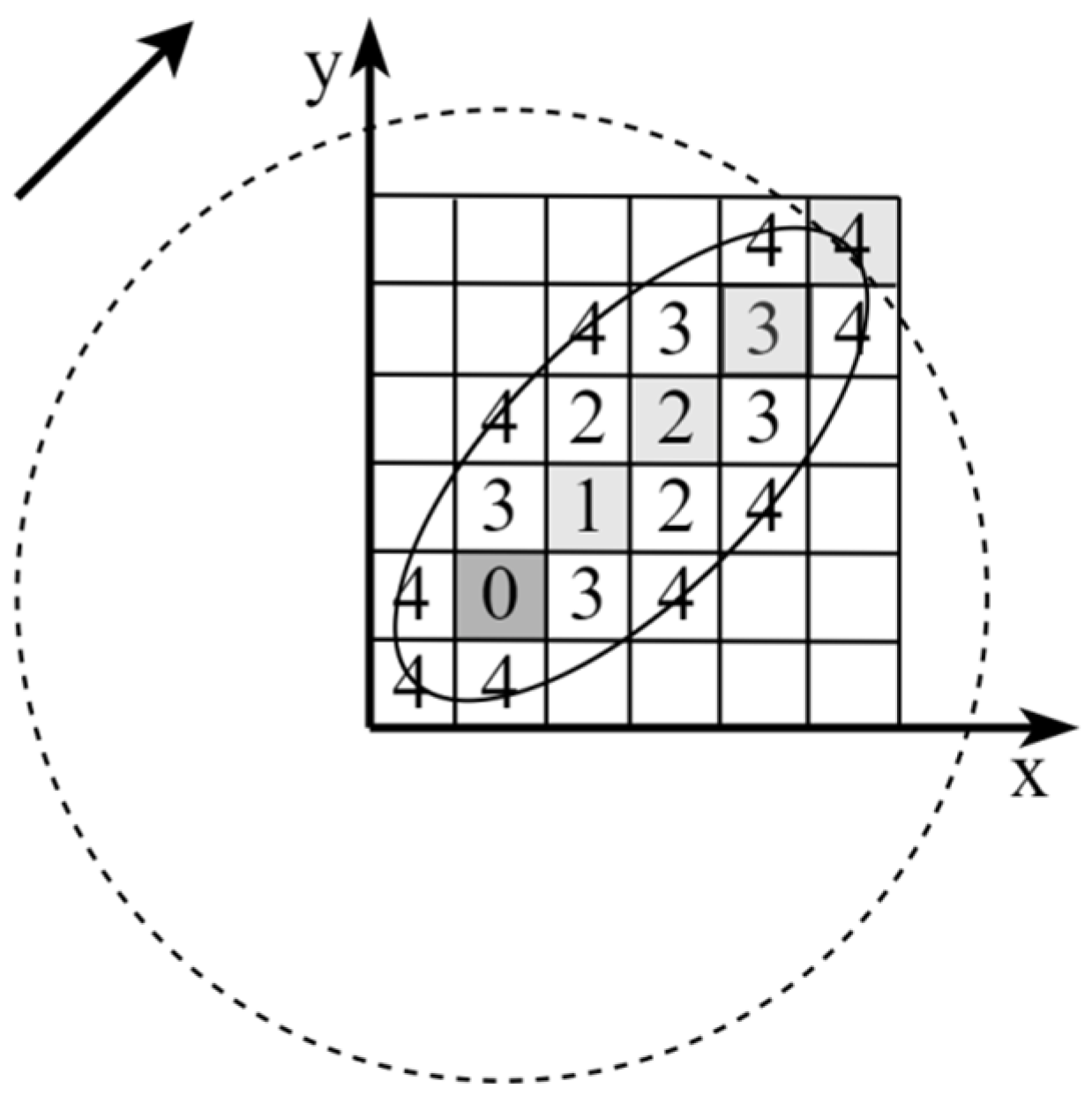
The distance field is illustrated in Figure 7, where the concentration isoline in the form of a circle is calculated using a simplified formula, and the isoline in the form of an ellipse is calculated based on the processing of experimental data. The concentrations on the emission axis are the same in both cases.

D. Martin [74] compares three models used to predict the concentration of a pollutant in an urban environment. The empirical model SUDC (The Simple Urban Dispersion Correlation), formed on the basis of experimental data and confirmed by aerodynamic tests, turned out to be the most suitable for describing the upper limit of concentration and was then chosen as the main model for calculating the concentration map.

The other two models (BUDM and ASUDM), based on Gaussian models, also show acceptable results, but they underestimate the pollutant concentration under wind channel conditions.

The transformation function Ψ₂: V × Y → Y is given by the SUDC Formula (15):

$$Y_x={\displaystyle \frac{QK{(S_x·c_{size})}^{-2}}{U}}$$

(15)

where Y_x is the pollutant concentration in the cell at ground level, kg/m³; S_x is the resulting distance from the emission source, m; Q is the intensity of the emission source, kg/s; U is the average wind speed, m/s; c_size is the cell size, m; K is the development factor (K = 3 in accordance with [75]).

The results of the simulation experiments showed that the main problems of the cellular automation approach to modeling the dispersion of pollutants are the problems of speed and numerical diffusion. To resolve the problems of speed, a frontal cellular automation algorithm with a hexagonal neighborhood pattern [76] was developed, in which the concentration front of the pollutant during the emission reaches and covers the barriers based on the probabilistic rules of frontal expansion. The frontal approach made it possible to accelerate the model calculations and reduce the processor time costs when calculating the contamination zone in the case of a complex configuration of barriers. However, in algorithms with peer-to-peer neighborhood patterns, the number of directions of angular transition is limited, which leads to the effect of numerical diffusion at different wind directions. It was determined that the procedures for generating random numbers significantly reduce the speed of calculations and lead to the appearance of “noise” in the modeling results. Therefore, in the developed empirical cellular automation algorithm [77], the Monte Carlo approach is not used, and to resolve the problems of numerical diffusion, a 16-point neighborhood pattern is used, which takes into account the features of the calculation scheme for finding the shortest path.

2.6. Selection of Forecast Algorithms and Visualization Examples

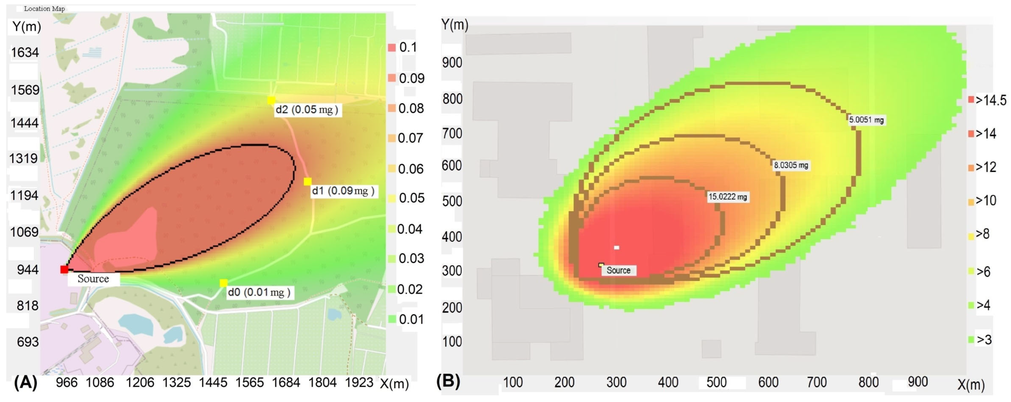
Figure 8 shows demonstration examples of the visualization of the area of contamination using the forecast algorithm based on the Gauss equation (A) and the probabilistic cellular automaton algorithm (B).

The analysis of the examples presented in Figure 8 showed that the forecasting algorithm based on the Gauss equation allows one to take into account the main dispersion factors for meso-scale accidents and ensures high speed of information processing when searching for the best solution. However, such an algorithm is not capable of accurately taking into account the complex dispersion conditions that arise for a local scale accident, including the effects of terrain development. The example (Figure 8B) demonstrates the possibilities of using a probabilistic cellular automaton algorithm that allows for taking into account the effects of terrain development in the visualization problem at distances less than 1 km, in comparison with solutions of the Gauss equation. However, in this case, problems of response time and numerical diffusion associated with the imitation of particle flight also arise. The problem of response time is caused by the need to generate and move an ensemble of test particles filling the surface cells taking into account the effect of interaction with obstacles. The discrete nature of the cellular automaton method, in contrast to Lagrangian models, does not allow for moving a particle in an arbitrary direction in one cycle, except for the directions leading to neighboring cells. The problem of numerical diffusion arises, which is most pronounced with a small standard deviation and different directions of particle flight that do not lead to neighboring cells of the neighborhood. These conditions lead to a distortion of the shape of the pollution cloud.

With distance from the emission axis, a “gradual approach of the Gaussian distribution curve to zero concentration” is observed, which complicates the averaged assessment of the plume boundaries. As a measure of the plume spread, it is advisable to use the deviation σ*, which characterizes the degree of dispersion of the emission relative to the plume center with the maximum concentration of contamination. The emission contours are formed on the basis of standard intervals of the deviation σ* [78].

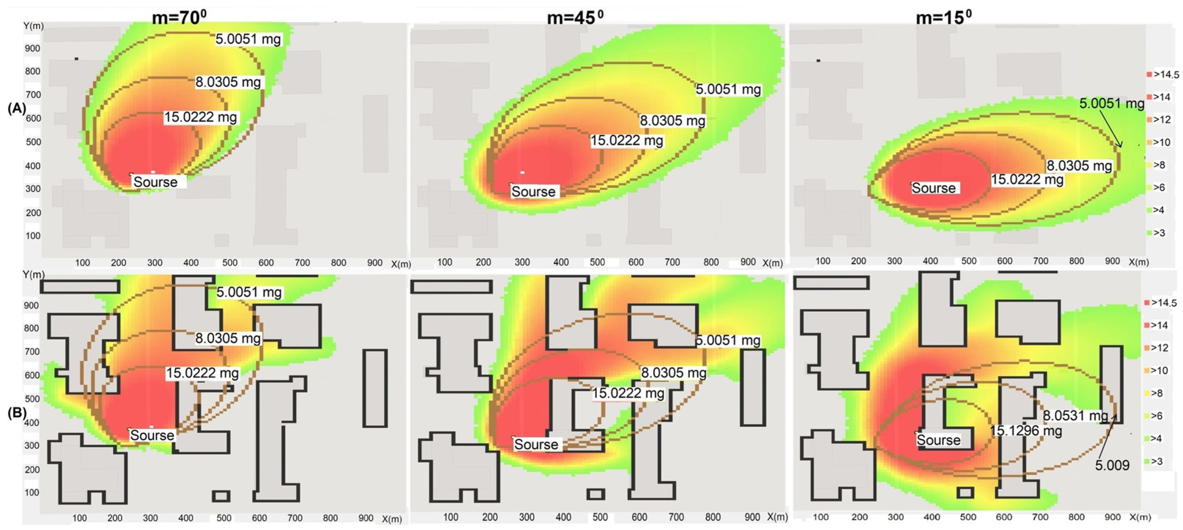
Figure 9 shows the dependences of the dispersion ellipse on the polar angle of the wind: A—without taking into account the development of the area; B—taking into account the effects of interaction with buildings. Simulation of the particle’s flight consumes a significant portion of the processor time, especially when the relief configuration becomes more complex.

The results of the simulation experiments showed that the procedures for generating random numbers significantly cause additional time expenditures in the processes of estimating the model parameters and lead to the appearance of “noise” in the modeling results. The problem arises of searching for modifications of the probabilistic algorithm of the cellular automaton for modeling diffusion taking into account the features and advantages of the empirical–statistical approach for visualizing the consequences of emergency emissions, which is described in detail in the authors’ publication [79].

2.7. Methodology for Visualizing Emissions of Hazardous Substances During a Fire at an Industrial Enterprise

The methodology for visualization and analysis of emergency emissions, developed on the basis of a generalized scheme of rapid response, is presented by the following stages of collecting and processing information:

• Formation of initial data for the forecasting and visualization of emergency pollution of the area. The initial data are data of the geographic information system with a digital map of the emergency zone; data of chemical reconnaissance of the area with coordinates of the location of measurements of hazardous substances concentration, as well as coordinates of the location of chemical pollution source; meteorological forecast data. If necessary, additional information is entered to determine the passivity of the emission.
• Selecting a forecasting algorithm. After entering the initial data into the system, a forecasting algorithm is selected depending on the scale of the accident, requirements for forecasting speed and accuracy, and the possibility of taking into account specific dispersion factors. The situation at the meso-scale level of an accident is assessed based on the Gauss equation. In this case, the effects of built-up area and the influence of wind fields are not taken into account. For an express assessment of the operational situation at the local scale of an accident, an empirical cellular automation algorithm is used, which ensures high computation speed under conditions of built-up area and the possibility of taking into account the wind field. If it is necessary to obtain more informative forecasts, then a cellular automation algorithm with imitation of a particle flight is used. An intermediate option is the frontal algorithm, which takes into account both the speed of operation and the effectiveness of forecasts.
• Calculation of the initial approximation. In the external circuit of the system, the parameters of the initial approximation necessary for the implementation of the solution search strategy are calculated. Based on the data of the geo-information system, a digital model of the obstacles required for calculating the forecast estimates under the conditions of built-up area is formed. Preliminary simulation experiments are carried out. The SUDC model is used to estimate the emission power Q* at a local scale of the accident.
• Application of the forecast parameter search strategy. Based on the criterial assessment of concentration deviations in observation–forecast pairs, the best forecast parameters are determined in a series of computational experiments. The process of determining the parameters is iterative and involves multiple calculations of the forecast with different parameters, which determines the time costs of searching for the reference solution. The forecast efficiency is assessed based on the geometric dispersion index VG. In the case of a forecast without taking into account wind fields, the performance of the probabilistic and frontal cellular automation algorithm is assessed using the FAC2 index. To search for forecast parameters based on the Gauss equation, the Simulated Annealing algorithm is used, the advantage of which is that it “ignores” the neighborhoods of local minima when searching for the best solution. To determine the forecast parameters based on the cellular automation approach, the Nelder–Mead and direct enumeration algorithms are used.
• Output of forecast results. The output information is a forecast assessment of the size and configuration of the area of contamination with a visual display of the boundaries of this area and profiles of the concentration of hazardous substances on a digital map of the area.

The results of forecasting and visualization can be used to analyze the chemical situation, adjust plans for localization and liquidation of the accident (and assess the effectiveness of emergency rescue operations based on current information about the accident, which ensures flexibility and adaptability of response to a changing situation.

2.8. Limitations and Difficulties of Using the Simulation Model and Ways to Overcome Them

The limitations of the application of the proposed simulation model of dangerous zone spread and the visualization of its boundaries are, first of all, the need to take into account a large number of factors (climatic, construction, the dynamics of the spread of fire) for the prompt construction of the contours of the dangerous zone. This complicates the creation of typical contours for the highly accurate forecasting of the spread of a toxic gas cloud for the early development of evacuation scenarios. It is also quite difficult to take into account the degree of toxicity of the emissions of combustion products into the atmosphere other than through their maximum permissible concentration.

We associate overcoming these limitations with the creation of a database with a large number of templates of dangerous zone contours for various scenarios of fire development at various industrial enterprises, with the ignition and explosion of chemicals of varying toxicity. To speed up the procedures of searching for a specific visualization of a dangerous zone for the closest conditions, it is advisable to use parallel computing algorithms. In this case, the problem of dividing the calculation field into separate flows is resolved. Full access to the shared environment is not provided to individual flows in the empirical cellular automation algorithm; each flow makes changes only to independent cells of the calculation grid based on data from neighboring cells.

3. Results

3.1. Software Visualization of Hazardous Substance Emissions During a Fire at an Industrial Enterprise

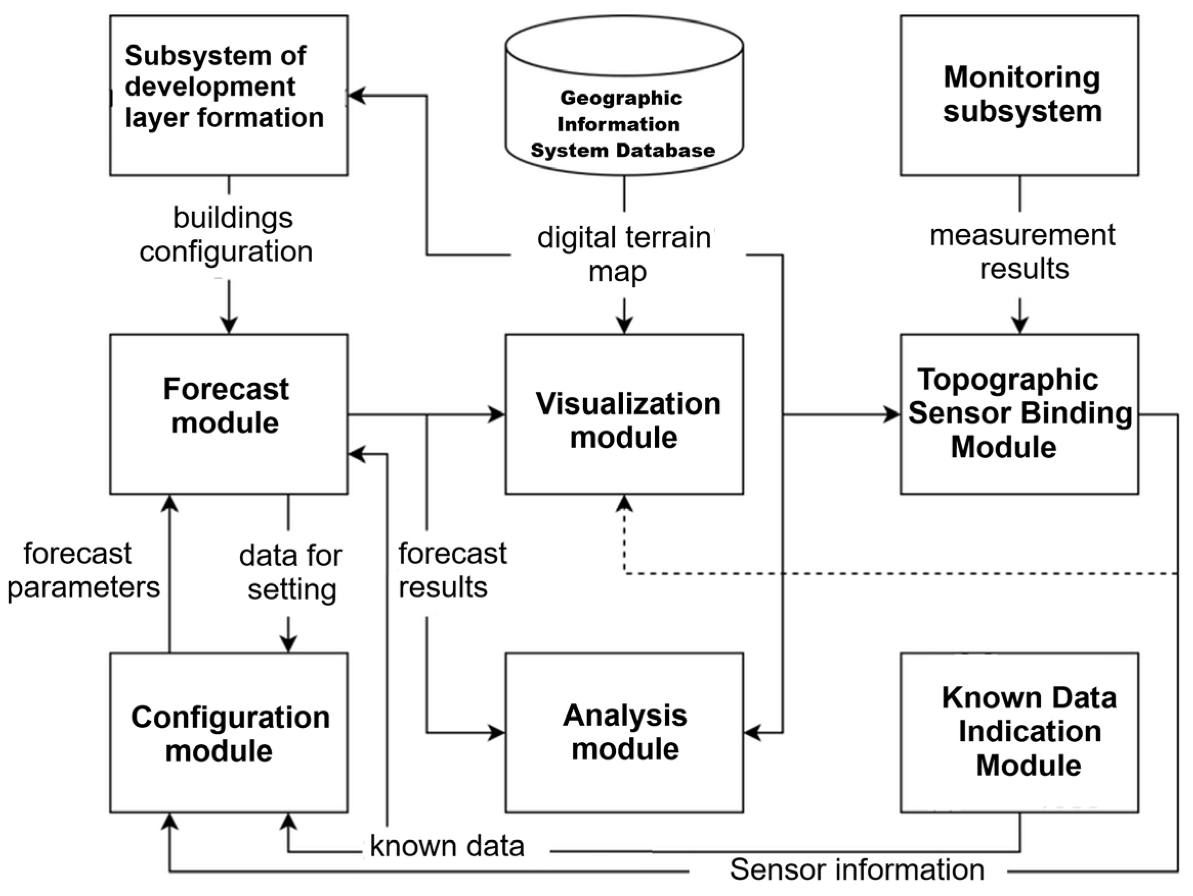
The structural diagram of the emission visualization is shown in Figure 10. The forecast module implements the modeling algorithm specified by the user and forms the resulting data of the hazardous chemical substances concentration fields C_i^m(x,y,z,t) at the fire site. It processes the information received from the a priori information input unit, including actual meteorological data and emission parameters (their possible expert scene). The module also requires information from the development configuration module, which converts the geographic information system data into a contour model of the terrain.

The data from the monitoring subsystem, containing information on the coordinates of the observation sensors and the results of measuring the concentration of hazardous substances at the observation sites C_i^m(x,y,z,t), are sent to the modules for calculating the parameters and topographic referencing of the sensors.

In the setup module, which implements the algorithms for global search and setting up the forecast parameters, the parameters P_var are selected based on the data from the monitoring system and the forecast module to ensure the minimum criterion assessment ∆₀. The results of the simulation experiment (with the best parameters) are transferred to the visualization module.

In the visualization module, the resulting model data (danger zone boundaries) are displayed on a digital map of the area, taking into account the topographic reference of the monitoring sensors. In the analysis module, a summary modeling result is generated.

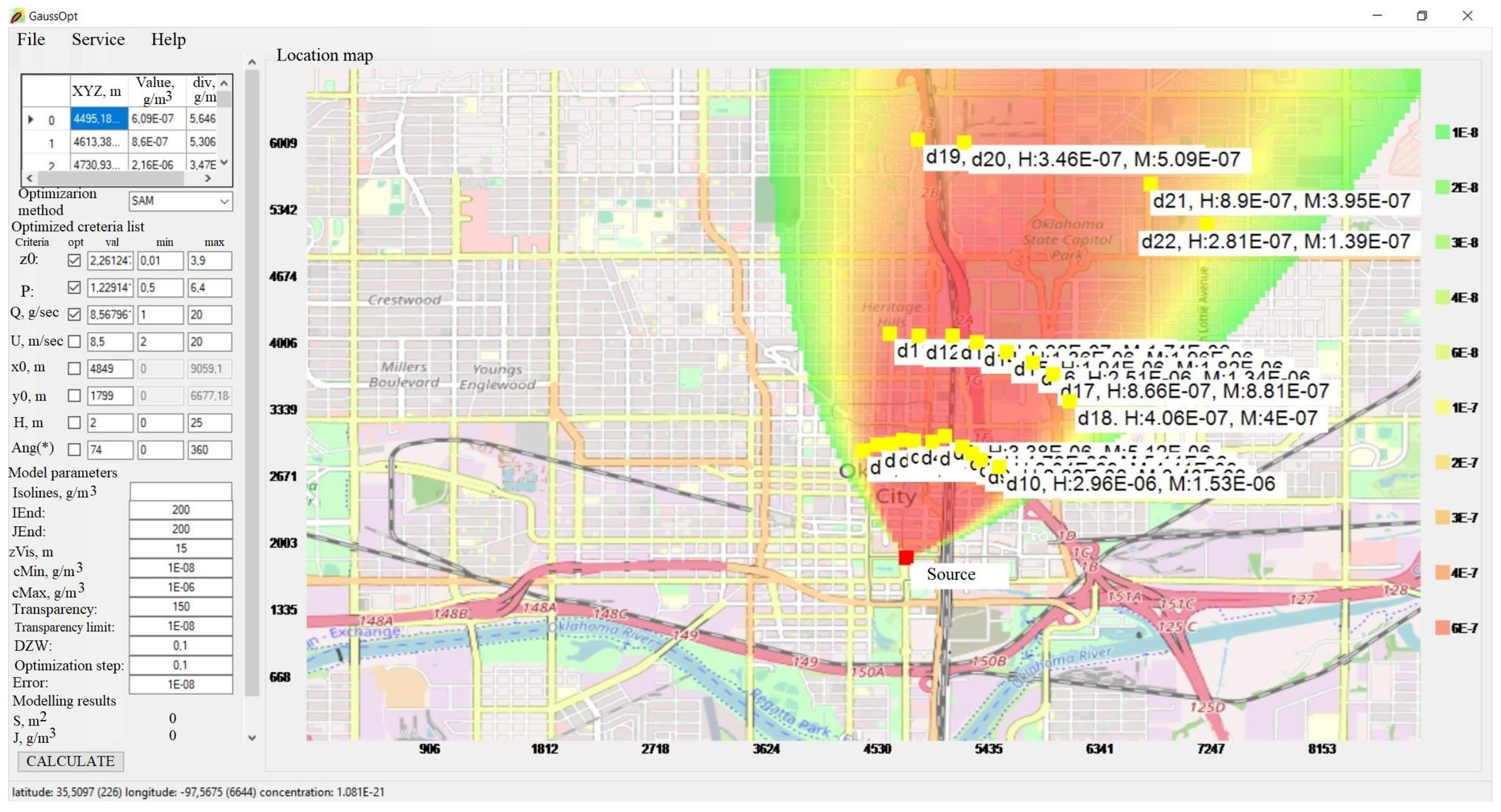
The prototype screen layout with the visualization of the concentration field with a forecast based on the Gauss equation at the meso-scale level of an accident is shown in Figure 11. In this picture, Ang* is the measured wind direction value.

This version of the program has the ability to autonomously load a map with its geographic coordinates. The program’s input/output functions are implemented based on the Windows Forms 9.0.6 application programming interface. The program window layout contains an algorithm setup area and an emission visualization area with the display of concentration fields of hazardous substances in the atmosphere.

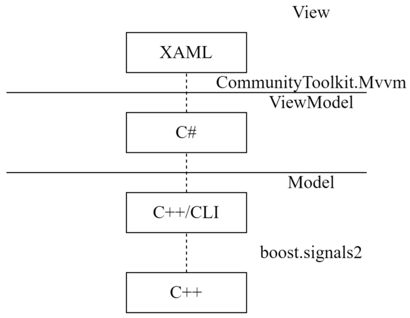
The program interface was developed using a forecast based on the cellular automation approach. The XAML markup language was selected for developing the program interface. The separation of application logic, user interface (UI), and data is based on the MVVM pattern.22. XAML is a declarative markup language used in WPF (Windows Presentation Foundation) applications, as well as in UWP (Universal Windows Platform) and Xamarin. Forms technologies. It allows for implementing a visual interface in the form of markup similar to XML. The MVVM pattern is the framework of the application. The model represents the business logic and data. The view is responsible for displaying the visual interface, and the ViewModel serves as a link between the model and the view. The mathematical core of the prototype is implemented based on the C++ programming language, which ensures high performance and efficiency of code execution. This choice also gave rise to additional development difficulties. Possible errors in memory management or incorrect optimization can lead to memory leaks and program instability. C++ does not have native support for events. The developed scheme of the interaction between the computing core and the user interface of the prototype is shown in Figure 12.

The events are implemented using a set of Boost libraries, which provide multithreading and efficient event processing. In particular, the Signals2 library is used, which is designed to implement signals and slots in the C++ language.

To work with the core written in C++, the C++/CLI or Managed C++ language was used, which provides tools for writing a bridge between the C++ code and the C# code. The CLI/C++ language implements a convenient way to integrate existing C++ code with .NET projects, especially in projects with unmanaged code or an API interface.

In the event of a fire, the generation of a detailed relief map when moving to the scene of the accident must be carried out with minimal time costs. At the stage of preparatory work, it is necessary to form a preliminary geospatial database of the emergency, containing terrain maps, a development scheme of the territory, information on roads and obstacles, etc. The main sources of information for such a database include geographic information systems (geographic information management tools) that allow for creating, editing, and analyzing spatial data. To build a model of barriers, it is necessary to use ready-made solutions that provide the user with graphic information about the configuration of buildings and structures in the pollution zone, such as Qlik GeoAnalytics v5.20.0, Bentley OpenCities Map 2023, QGIS 3.16, OpenStreetMap Online, ArcGIS Pro 2.8, MapInfo Pro 2011, etc.

3.2. Results of Visualization of Hazardous Substances Emission During Fire

In the project of forecasting the dispersion of accidental emissions based on the Gauss algorithm, the target function of the adjustment is formed based on a limited number of reference measurements. Therefore, no significant requirements were put forward for the development of the project. After installing the 32-bit version of the project on a laptop with an Intel Core i5-6200U processor, about 2 s of processor time were required to implement the “Annealing Method” procedure with four reference measurements. With an increase in the number of reference measurements, the processor time costs increase to 5–10 s. The amount of RAM required for the project is 43 MB.

The prototype of the hazardous substance emission visualization system based on the probabilistic cellular automation is currently limited by the framework of a two-dimensional computational grid. With a grid resolution of 150 × 150 cells, the program consumes about 40 MB of RAM. The prototype operates under Windows 7–11 with pre-installed .NET framework 4.0. The total program size is 1.83 MB. Reducing the procedures simulating the particle flight led to a decrease in the time spent on finding a reference solution. The results were processed on a mobile Intel(R) Core i5-6200U CPU @ 2.30 GHz (two cores, four logical processors).

The experimental study of the developed algorithms was carried out using the data from field tests of the Joint Urban 2003 (JU03) pollution indicator (Pacific Northwest National Laboratory, Richland, Washington, DC, USA) [80], which are the basis for numerous scientific studies on environmental monitoring. The field measurement information used below is provided as “public domain” and refers to creative materials that are not protected by intellectual property laws such copyright, trademark, or patent laws.

When selecting the initial data, the emission scale limitations were taken into account. For testing the dispersion forecast subsystem based on the Gauss equation, concentration measurements located at a distance of at least 1 km from the emission source were used; for testing the forecast subsystem based on the cellular automation approach, a distance of no more than 1 km from the emission source was used.

When analyzing the field test data of the Joint Urban 2003 (JU03) pollution indicator, the following rule for selecting reference measurements was applied: Measurements with a concentration level of c^d_x ≤ 45 pptv were considered uncertain.

The following data sets were used to visualize the hazardous area:

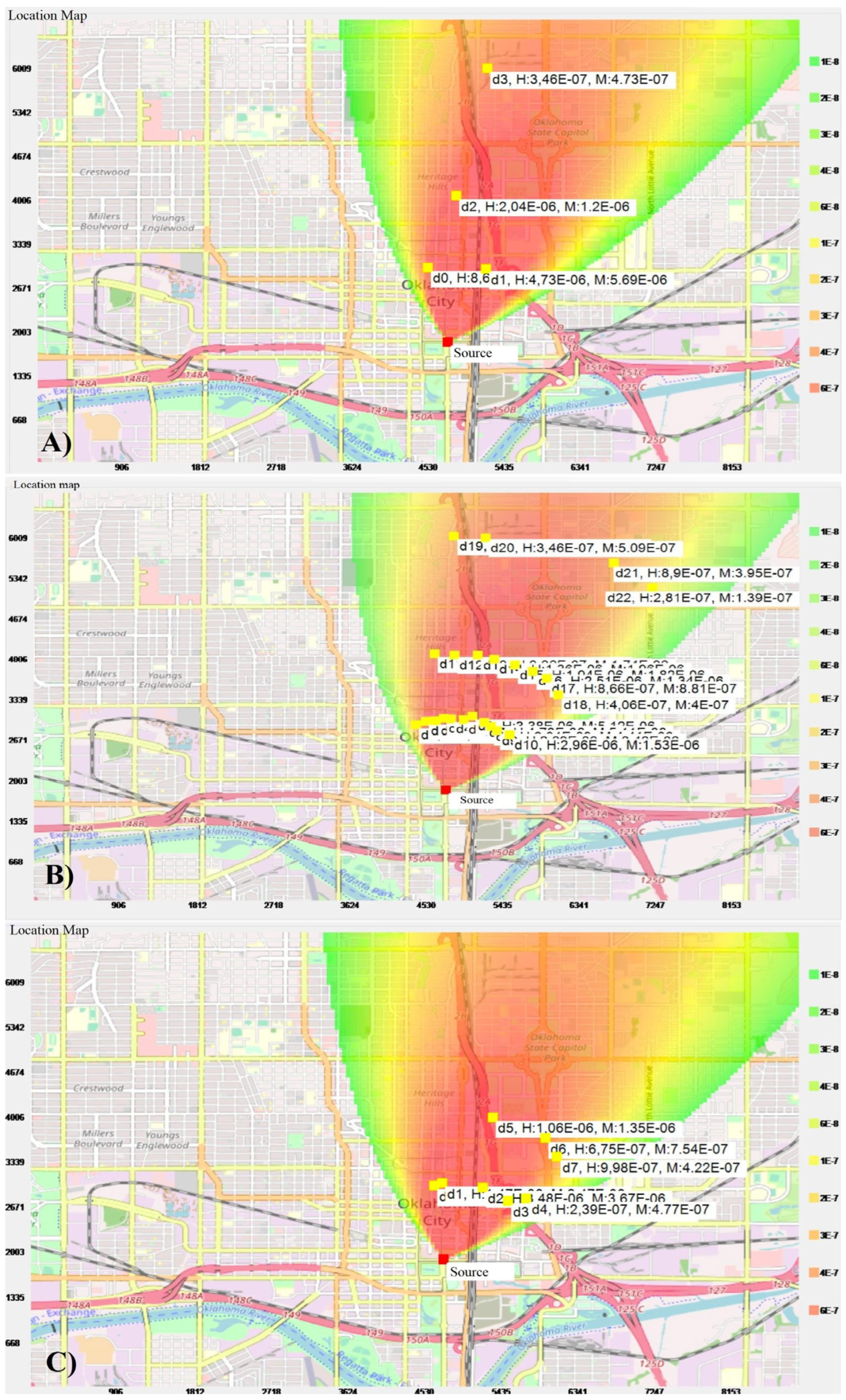
(A)

Data Set 1: fire area—600 sq. m; duration of intense burning—3 h; average wind speed at the fire location—4 m/s; emission power of evaporated harmful combustible materials—320 kg (toluene, styrene, dioxins—up to 90% by weight in the air); Q = 1.27 × 10⁻⁷ kg/s; fire height—2 m.

(B)

Data Set 2: fire area—750 sq. m; duration of intense burning—3.5 h; average wind speed at the fire location—3 m/s; emission power of evaporated harmful combustible materials—320 kg (toluene, styrene, dioxins); Q = 1.27 × 10⁻⁷ kg/s; height of fire source—2.5 m.

(C)

Data Set 3: fire area—650 sq. m; duration of intense burning—3 h; average wind speed at the fire site—5 m/s; emission power of evaporated harmful combustible materials—320 kg (toluene, styrene, dioxins); Q = 1.27 × 10⁻⁷ kg/s; height of fire source—3 m.

The visualization results of hazardous substance emissions during a fire, plotted on a conventional terrain map, are shown in the following figures:

-

To visualize the forecast for the spread of a hazardous area based on the Gauss equation for Data Sets 1, 2, and 3—Figure 13 and Figure 14. The units of measurement on the terrain map are feet.

-

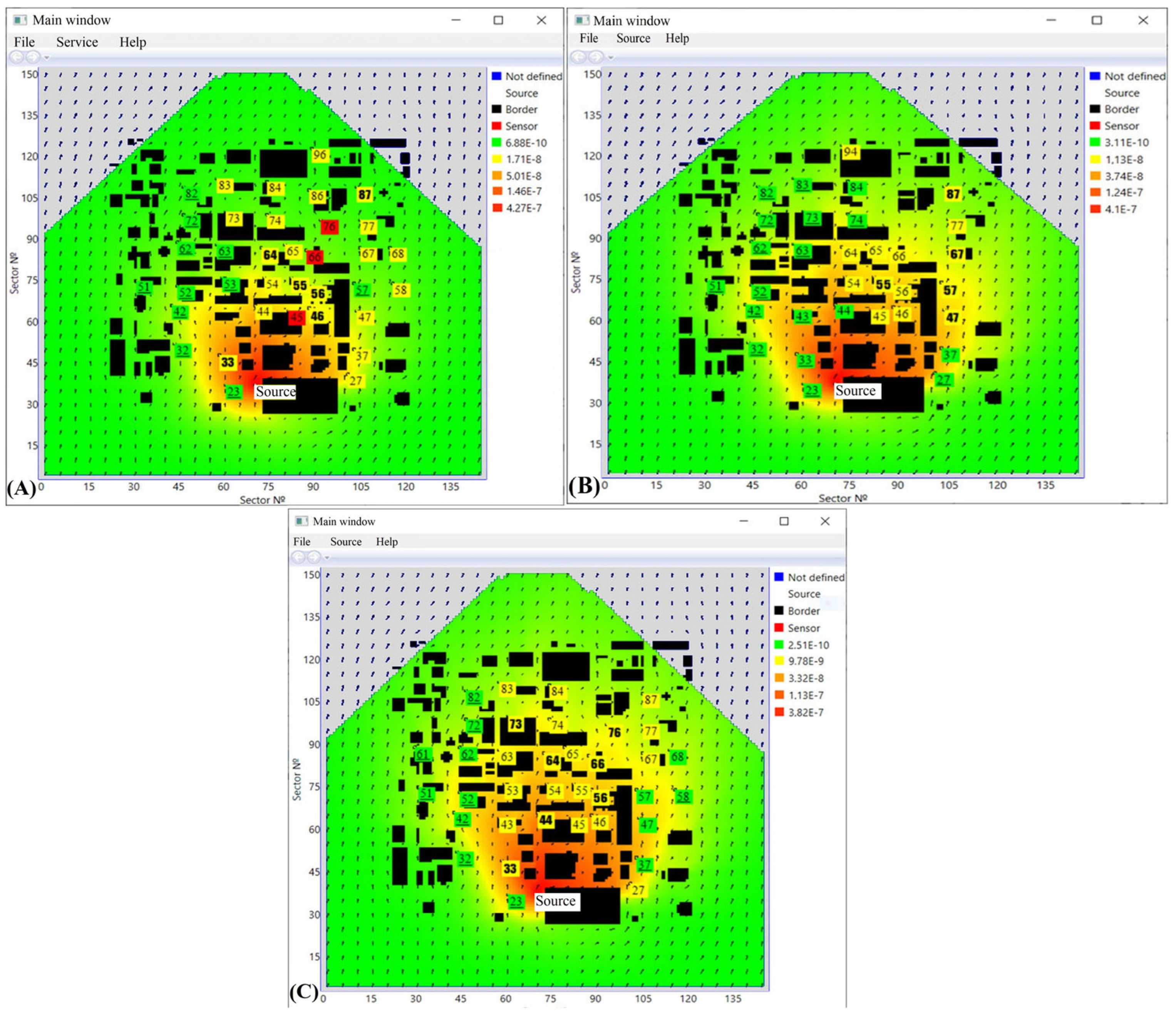
To visualize the forecast for the spread of a hazardous area based on the probabilistic cellular automation approach—Figure 15 and Figure 16. The units of measurement on the terrain map are meters. The average height of buildings is 22 m, the tracer emission power is Q = 1.27 × 10⁻⁷ kg/s.

Figure 13 shows the visualization of the emission area and the spread of the hazardous area based on the Gauss equation using the three data sets.

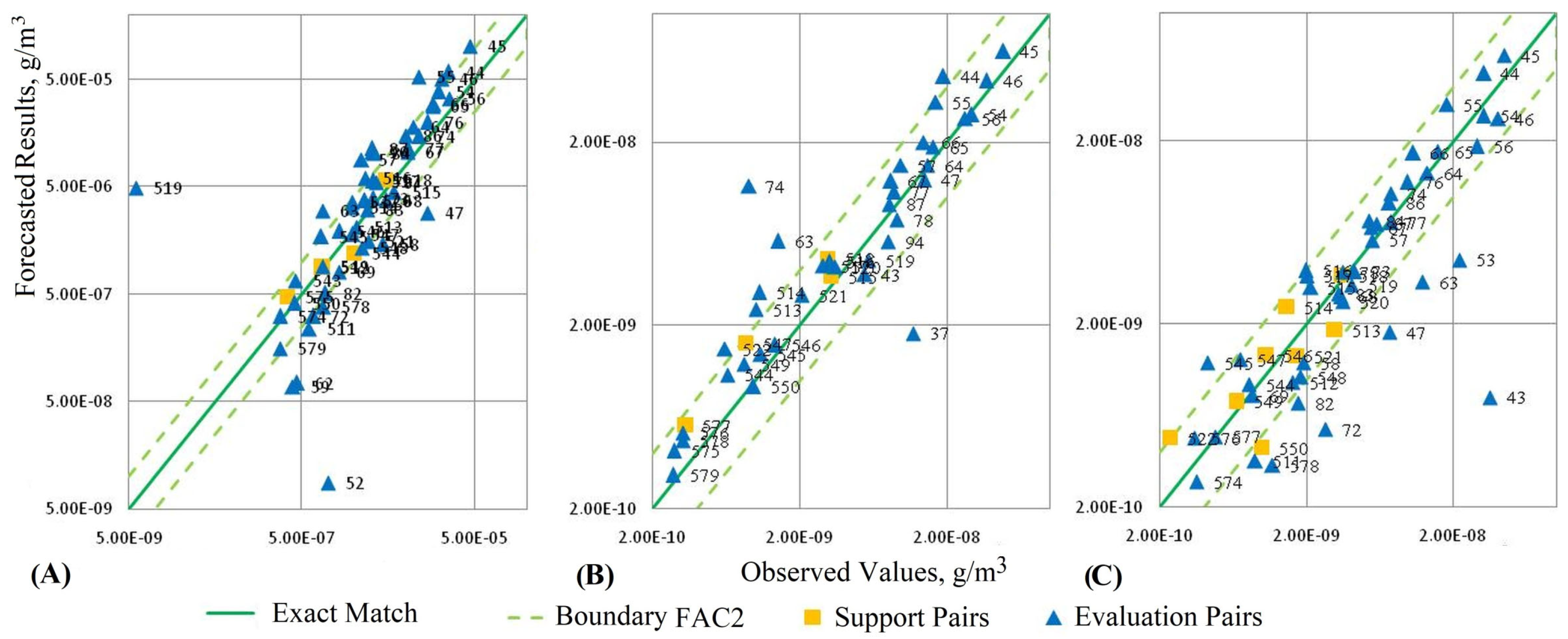
Figure 14 shows the resulting diagram of the pairs “observation–forecast” of the concentration level of hazardous substances based on the Gauss equation using the three data sets.

In Figure 14, square markers denote the reference pairs used for parametric tuning of the forecast models, and triangular markers denote the pairs used to evaluate the performance of the forecast algorithms. The solid line “Exact match” in the resulting diagrams corresponds to the ideal forecast variant, in which the predicted values coincide with the concentration measurements. Two dotted lines denote the boundaries of the range within which the pairs are considered satisfactory according to the FAC2 criterion (the proportion of pairs falling within the range boundaries out of the total number of such pairs).

Figure 15 shows the visualization of the hazardous area based on the cellular automation approach for three data sets.

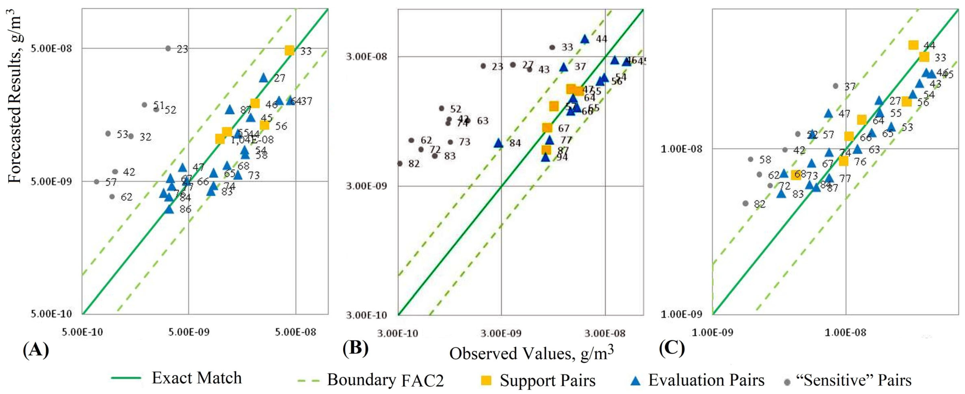
Figure 16 shows the resulting diagram of the pairs “observation–forecast” of the concentration level of hazardous substances based on the cellular automation approach for three data sets.

Square, round markers, solid and dotted lines in Figure 16 mean the same as in Figure 14. In addition, round markers denote “sensitive” pairs, which were also taken into account when calculating the forecast performance indicators. Using such “sensitive” variants as reference pairs leads to forecast errors and distortions of the visualization results.

According to S.D. Sabatino, R. Buccolieri et al. [81], the following generally accepted intervals of criterion indicators are characteristic of the “modern” forecast model (Fractional Bias (FB), the Normalized Mean Square Error (NMSE), the fraction of predictions within a factor of two of observations (FAC2), the Geometric Mean (MG) bias and the geometric variance (VG)). The limits of these indicators are the following: –0.3 < FB < 0.3; NMSE < 4; FAC2 ≥ 0.5; 0.7 < MG < 1.3; VG < 1.5.

Table 1. Summary table of forecast efficiency.

Forecast Indicators	FB	MG	NMSE	VG	FAC2
Gaussian (over 1 km, excluding built-up effects), JU03, Data Sets 1, 2, 3
Average value (running time 5 s)	−0.24	0.94	1.12	3.52	0.72
Probabilistic cellular automation algorithm (up to 1 km taking into account the effects of built-up terrain), JU03, Data Sets 1, 2, 3
Average value (running time 158 s)	0.08	1.06	0.17	1.44	0.85
Empirical cellular automation algorithm (up to 1 km taking into account the effects of built-up areas), JU03, Data Sets 1, 2, 3
Average value (running time 11 s)	−0.20	0.55	0.87	7.11	0.52

presents the summary information obtained as a result of the control test of the system. When calculating the FB, MG, NMSE, VG criteria, the formed observation–forecast pairs corresponding to the selected measurements were taken into account. The table highlights the values of the indicators that satisfy the conditions of an effective forecast.

The analysis of the summary information presented in Table 1 showed that most of the values of the criterion indicators calculated as a result of testing the developed forecast and visualization algorithms generally correspond to the above requirements. The forecast subsystem based on the Gauss equation is operational under conditions of stable wind at the macro- and meso-level scale of accidents. The forecast subsystem based on the cellular automation demonstrates operability under conditions of built-up terrain and is capable of taking into account the influence of the wind field on the configuration of the emission area. For each cell of the modeling area, it is necessary to set the mathematical expectation and variance of the wind direction. The standard deviation remains a variable parameter, and for each cell a correction coefficient is introduced into correspondence, taking into account the relative wind speed.

It has been determined that the efficiency of forecasting using cellular automation algorithms is greatly affected by wind flow prediction errors. Such errors are associated with a simplified approach to wind flow modeling, in which the same boundary conditions are specified at the boundaries of the computational domain, which is a rough approximation of the actual conditions, which are characterized by heterogeneity and temporal variability.

The analysis of the results of the visualization of dangerous zones and the comparison of the actual concentration of harmful combustion products with the actual measurements, shown in Figure 12 and Figure 13, allowed us to draw the following conclusions.

The design of dangerous zones based on the Gauss equation is preferable under conditions of stable wind during large-scale fires outside dense buildings or other obstacles (e.g., forest plantations or complex terrain). In contrast, the visual forecast based on the cellular automation approach demonstrates operability under conditions of dense buildings or complex terrain and can take into account the influence of the wind field on the configuration of the emission area.

In general, the comparison of the results of the visualization of hazardous zones of harmful combustion product spreads, modeled on the basis of the Gauss equation and the empirical cellular automation approach, allows us to conclude that the latter is more accurate. This is achieved, first of all, by taking into account obstacles in the form of buildings and structures of known spatial location, as well as more accurate imitation of the flight of particles. Therefore, visualization based on the Gauss method is more suitable for forecasting and visualizing the hazardous pollution zone at the macro- and meso-level scale of fires, and based on the cellular automation approach for more localized incidents with highly toxic emissions.

4. Discussion

The study resulted in the development of recommendations for the application of Gaussian and cellular automation algorithms for the visualization of hazardous zones of harmful substances emitted into the atmosphere during fire at industrial enterprise, used in forecasting based on prototype software running under Windows OS with preinstalled .NET framework 4.0. The comparison with field measurements of hazardous substance concentrations in the cloud showed different applications for the used methods—Gaussian for forecasting the spread of harmful substance clouds during full-scale, large-scale fires outside densely built-up areas, and cellular automation approach for more localized fires in densely built-up areas or complex terrain. Compared with traditional approaches, which determine the percentage of direct correspondence of “forecast–observation” pairs, the cellular automation approach takes into account possible variations in parameters. If the results of the actual measurement of forecast parameters are within the established limits, then such forecasts are considered stable in the specified range of parameter variations.

The approach to solving this problem is the decomposition of the criterion evaluation function on a set of reference measurements. Based on the enumeration method, a response function is formed for each observation–measurement pair to evaluate all possible combinations of the variable parameters. The response is represented by the ratio of the concentration in the observation–forecast pairs. A measurement is declared sensitive if the number of parameter combinations leading to a more than 5-fold deviation of the values in the observation–measurement pair is more than 75% of the total number of combinations.

Compared to traditional approaches that determine the percentage of direct correspondence between forecast–observation pairs, this approach takes into account possible variations in the parameters. If the results of scanning the forecast parameters are within the established limits, then such forecasts are considered stable in the specified range of parameter variation.

The practical value lies in the attempt to combine the forecast system based on the Gauss equation, which is operational under conditions of stable wind at the meso-level scale of accidents, with the forecast system based on cellular automation, which demonstrates its operational capability under conditions of built-up terrain and is capable of taking into account the influence of the wind field on the configuration of the emission area. Algorithms of the cellular automation forecast model have been developed and implemented in software, which differ in taking into account the rules for filling the dispersion ellipse, as well as the effects of interaction with obstacles, which allows for a more accurate mathematical description of the spread of pollution under conditions of built-up terrain.

5. Conclusions

This article analyzes the capabilities and limitations of the well-known Gaussian approach, as well as the cellular automation approach for developing a method for predicting and visualizing the hazardous zone of toxic combustion product propagation during a fire at an industrial enterprise, with the ability to adjust the forecast parameters when weather conditions change. For this purpose, the features and conditions for applying the algorithms for predicting the propagation of the hazardous zone (based on the Gaussian equation, as well as probabilistic, frontal, and empirical cellular automation) were analyzed for implementation in the internal loop of the fire consequences visualization and analysis system. As a result, algorithms for the cellular automation model for the visual prediction of the hazardous zone were developed and software implemented. This differs in taking into account the rules for filling the dispersion ellipse, as well as the effects of interaction with obstacles, which allows for a more accurate mathematical description of the propagation of a cloud of toxic combustion products under the conditions of a built-up area.

An approach to the development of algorithmic capabilities of the integrated system is proposed, featuring the ability to visualize the emission area using wind flows based on the frontal and empirical modification of the cellular automation model algorithms, which significantly allows for speeding up model calculations under conditions of a complex relief configuration and high detail of the terrain map. An algorithm for generating a digital terrain model is implemented, which differs from the existing ones in the method of generating contours of objects distributed beyond the boundaries of the autonomous map. Software and algorithmic support for an integrated system for the visualization and analysis of the consequences of a fire at an industrial enterprise has been developed; the efficiency of the system has been confirmed by computational experiments and testing results.

It is concluded that the application of the Gauss equation for designing hazardous areas has advantages in large-scale fires outside densely built-up areas, preferably under conditions of stable wind. Under conditions of dense urban or industrial development, complex terrain and variable wind field, the visualization of the hazardous area during a fire at an industrial enterprise based on a cellular automation approach is more accurate.

The practical application of the developed algorithms will expand the capabilities of verified software tools, accelerate and simplify the analysis of an emergency situation under complex emission conditions at a local and meso-scale level of contamination of the area.