Abstract
In this study, we investigated the influence of pre-fire tree mortality on fire behavior. Although other studies have focused on the environmental factors affecting wildfire, the influence of pre-fire tree mortality has not been explored in detail. We used high-spatial-resolution (1.6 m) airborne multispectral orthoimages to detect and map pre-fire dead trees in a portion of the San Bernardino Mountains, where the ‘Old Fire’ burned in 2003, and assessed whether spatial patterns of fire intensity and burn severity coincide with patterns of tree mortality. Dead trees were mapped through a hybrid deep learning classification and manual editing approach and facilitated with Google Earth Pro historical images. Apparent thermal infrared (TIR) brightness temperature captured during the Old Fire was derived from maximum digital number values from FireMapper airborne thermal infrared imagery (7 m) as a measure of fire intensity. Burn severity was analyzed using normalized burn ratio maps derived from pre- and post-fire Landsat 5 satellite imagery (30 m). Pre-fire dead trees were prevalent with 192 dead trees and 108 live trees per ha, with most dead trees clustered near the northwestern part of the study area east of Lake Arrowhead. The degree of spatial correspondence among dead tree density, fire intensity, and burn severity was analyzed using graphical and statistical analyses. The results revealed a significant but weak spatial association of dead trees with fire intensity (R2 = 0.31) and burn severity (R2 = 0.14). The findings revealed that areas impacted by pre-fire tree mortality were subject to higher fire intensity, followed by severe burn effects, though other biophysical factors also influenced these fire behavior variables. These results contradict a previous study that found no effect of tree mortality on the behavior of the Old Fire.
1. Introduction
Pre-fire tree mortality refers to the dieback of trees prior to a fire primarily due to drought, insect infestation, thunderstorm, or disease [1,2]. The dry fuel loads from standing dead trees can contribute to large wildfires by increasing dead biomass in the forest [3]. Pre-existing dead trees also influence fire behavior and subsequent burn severity. Moreover, dead trees act as ladder fuels, which can be responsible for spreading the fire from the ground to the tree canopy [4]. Dead fuel loads can also influence fire spread by enhancing the ignition of spot fires [5]. Petropoulos and Islam (2017) noted that the volume of flammable material and the arrangement of fuel can increase fire spread and severity [6].
Wildland fires are common in southern California landscapes due to its seasonally dry, semi-arid climate; mountainous topography; and flammable vegetation [7]. Keeley (2009) stated that the wildfires in Southern California cause great damage to personal safety and assets [7]. The spread of human settlement near and within the fire-prone vegetation of the wildland urban interface and the excessively long duration of droughts are also responsible for the vulnerability of southern California residents to fire [8]. Most wildfires in the southern California region are ignited by human activity such as power line failure, arson, camping, etc. [9].
The San Bernardino National Forest suffered a widespread mortality event after prolonged drought in the early 2000s [10]. Subsequently, three major fires within southern California started on 25 October 2003, burning thousands of hectares of lands and homes in southern California: The Old Fire, the Cedar Fire, and the Grand Prix Fire [11]. Lake Arrowhead, Crestline, the city of San Bernardino, and Running Springs were threatened by the Old Fire (USFS, 2003). Some have speculated that the behavior of the Old Fire may have been influenced by the substantial presence of dead trees [11]. While Bond et al. (2009) assessed the relationship between tree mortality and burn severity derived from remotely sensed data, vegetation characteristics such as types, dominant tree, canopy cover, and topographic features like slope and aspect, they did not map tree mortality at the individual dead tree level and used crude estimates of dead tree density based on real-time visual estimates from spotters in helicopters [12]. In this paper, we use a hybrid automated–manual approach of dead tree mapping. Moreover, the Bond et al. (2009) study did not assess the influence of tree mortality of fire behavior, whereas we analyze influences on fire intensity. We also assess potential linkages of tree mortality to fire intensity based on remotely sensed data and post-fire burn severity analysis [12].
Investigating the role of dead tree cover on fire behavior and burn severity requires data collection before, during, and after a fire event, which can all be gathered with different methods of remote sensing. Remote sensing offers efficient means of collecting suitable data for pre-fire tree mortality assessments [13]. Specifically, high-spatial-resolution airborne imagery is an effective data source for detecting individual trees and the canopy of groups of trees to assess pre-fire dead tree cover [14]. The FireMapper thermal imaging radiometer of the USDA Forest Service captured high-resolution airborne imagery during the October 2003 fires in southern California. Extensive forest mortality due to bark beetle infestation and droughts were observed from the imagery from the Old and Cedar fires [11].
During the wildfire, aerial thermal infrared (ATIR) images provide relevant information about active wildfire that is useful to study the dynamics of wildfire behavior, such as fire intensity and rate of spread [15]. Fire intensity is known as the release of energy at the fire front, per unit time per unit length [7,16]. Burn severity is defined as a measurement of fire severity on the ground, particularly changes in the physical and ecological environment caused by fire activity [17]. Normalized burn ratio (NBR) and delta normalized burn ratio (dNBR) are useful spectral indices for mapping the extent of the burned area and estimating burn severity using pre- and post-fire imagery [7]. In particular, a combination of pre- and post-fire Landsat 5 TM+ and aerial multispectral orthoimages is commonly used to generate NBR and dNBR images that can be classified into different categories of burn severity using established methods [18]. High-spatial-resolution (1.6 m) aerial orthoimages including visible, near infrared (NIR), shortwave infrared (SWIR), and thermal infrared (TIR) were provided by collaborators in the USDA Forest Service. This dataset offers pre-, during, and post-fire images which were captured, processed, and made available for this study, providing a unique opportunity to study all phases of a wildfire.
In this study, we used high-spatial-resolution (1 m) airborne multispectral orthoimages to detect and map tree mortality for a portion of the San Bernardino Mountains, where the Old Fire burned in 2003, and analyzed the spatial association of dead trees with the intensity and burn severity of fire. We used brightness temperature values from ATIR images as a proxy for fire intensity. We mapped patterns of burn severity based on the satellite-derived NBR and dNBR index. To explore the role of dead tree cover on fire intensity and burn severity, we examined the spatial association of pre-fire dead tree density (number of trees per unit area) derived for 90 m × 90 m grid cells with ATIR-derived fire intensity (7 m spatial resolution) and Landsat-derived burn severity (30 m spatial resolution) using spatial analysis and statistical methods.
This study was built on the hypothesis that the presence and density of pre-fire dead trees increased the fire intensity and post-fire burn severity of the Old Fire, focused on a forested area east of Lake Arrowhead [11]. The research will enhance a better understanding of fire management practices in future wildfire scenarios.
Within the context of the 2003 Old Fire, this study aimed to address the following questions:
- How were pre-fire dead trees spatially distributed throughout the San Bernardino Mountain study area prior to the fire?
- Is fire intensity, as represented by ATIR apparent brightness temperatures, spatially associated with pre-fire dead tree density?
- Is burn severity, as represented by Landsat 5 TM dNBR imagery, spatially associated with patterns of pre-fire dead trees? How does the burn severity vary in areas with higher numbers of dead trees compared to areas with lower numbers of dead trees?
2. Methods
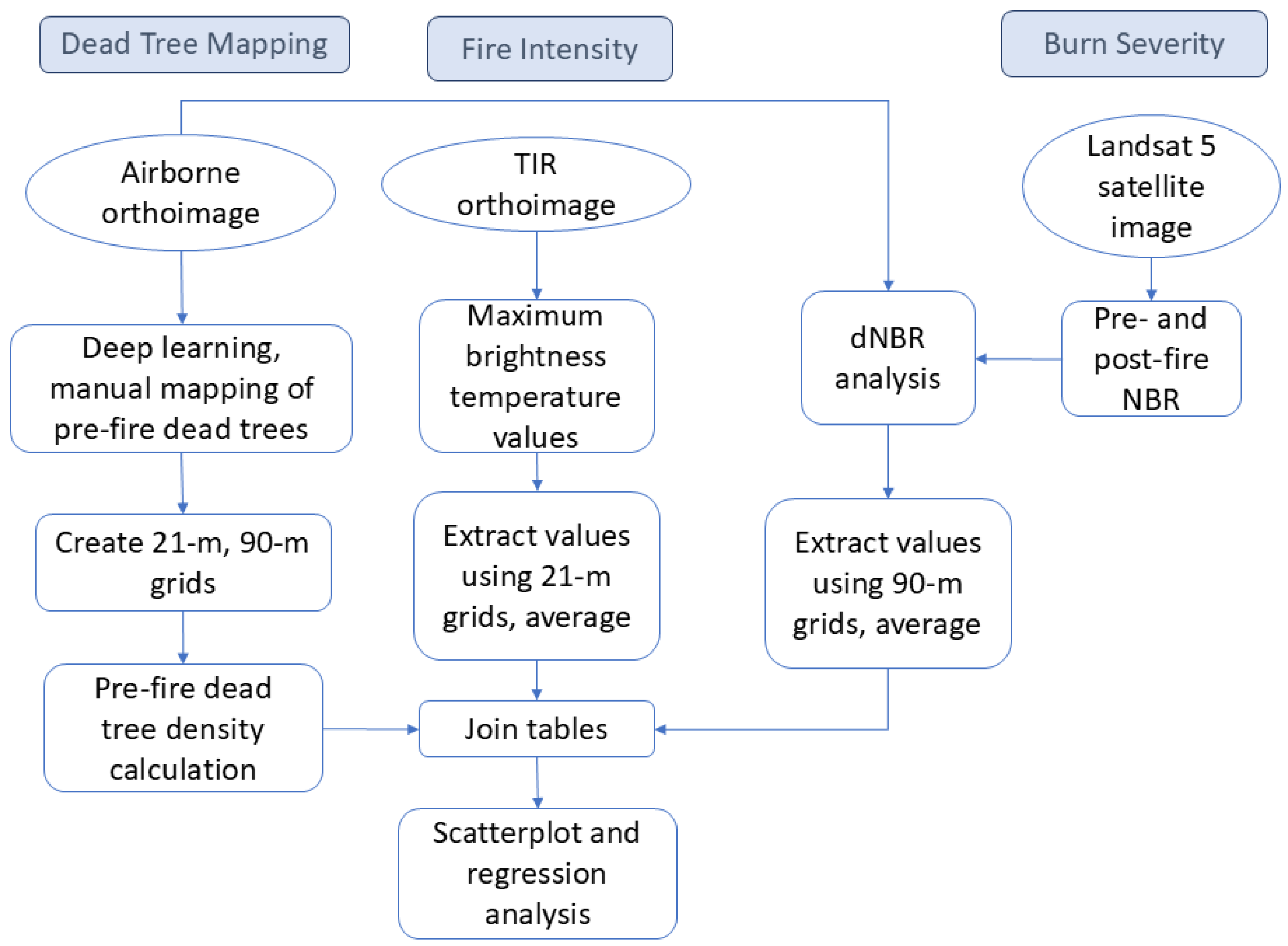
This study is primarily based on airborne imagery collected by the USDA Forest Service Pacific Southwest Research station before, during, and after the Old Fire in 2003 in the San Bernardino Mountains. To address the research questions, airborne multispectral imagery was used for mapping pre-fire dead trees, ATIR images for active fire intensity analysis, and post-fire Landsat data for determining post-fire burn severity. We analyzed the spatial distribution of fire intensity and burn severity with pre-fire dead trees with scatter plot and regression analysis. A flowchart for the general research approach and procedures is shown in Figure 1.
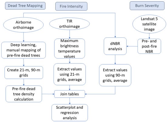
Figure 1.
Data and methods flowchart. TIR: thermal infrared, dNBR: delta normalized burn ratio.
2.1. Study Area
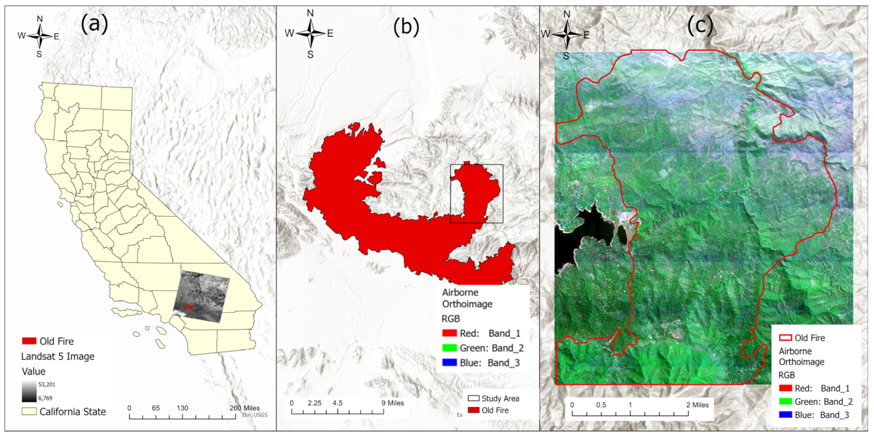
The study area for this research corresponds to parts of the lands which burned during the Old Fire, as shown in Figure 2. Beginning on 25 October 2003, the Old Fire burned about 23,000 ha in the San Bernardino Mountains until 5 November 2003 [19,20]. It burned during high wind and low relative humidity conditions of a Santa Ana weather event, which is common for fall fires in the southern California region [21,22]. The Old Fire burned a substantial amount of chaparral and woodland vegetation in low and high elevated areas, respectively [20]. The study area is mainly composed of coniferous forest, chaparral, black oak and canyon oak woodlands, and riparian vegetation. The study area has a Mediterranean climate which results in hot, dry summer and wet winter seasons [1].
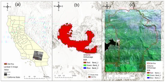
Figure 2.
Study area delineated by Old Fire 2003 in San Bernardino, CA, USA. (a) Pre-fire Landsat 5 image of the Old Fire overlayed on a county map of California. (b) The Old Fire burned area with bounding rectangle covering the specific study area. (c) Multispectral airborne orthoimage of the study area containing portions of Old Fire perimeter.
The San Bernardino National Forest contains a wide array of ecosystems and vegetation communities including montane mixed conifer forests, which are dominated by tree species such as Jeffrey pine, white fir, sugar pine, canyon live oak, and black oak [1,23]. It hosts diverse species of plants and animals, particularly deep-rooted chaparral shrubs along with mixed conifer forests in higher-elevation areas [12,19]. Conifer forests occur at elevations between 1400 and 2600 m and occupy a range of 57,000 ha in the San Bernardino Mountains [24]. Fire return interval (FRI) in the Old Fire burn area typically varies from 10 to 35 years. However, the area has experienced significant departure from the FRI historically, with approximately 55% of the forest burning either more or less frequently. The coniferous forests in the study area experiencing low-severity fires every 0–35 years are burning less frequently at present, which increases their vulnerability to severe fires [25].
2.2. Data Collection
High-spatial-resolution airborne imagery was collected prior to and following the Old Fire, processed, provided as orthoimage mosaics by USFS PSW Research Station, and used to detect and map dead trees for this study. The red NIR bands of the orthoimages have a spatial resolution of 1.6 m. These four waveband aerial frame images were taken from November 2002 to September 2003 (prior to the Old Fire), October 2003 (active fire), and November 2003 (after the Old Fire) in the visible red (0.62 to 0.69 μm), NIR (0.82 to 0.89 μm), SWIR (1.6 μm), a narrow TIR (11.4 to 12.4 μm), and a wide TIR (8.1 to 12.5 μm) bands. The images were processed using Agisoft Metashape software version 2.1.0 to create a digital surface model and orthoimages. Details of image data are provided in Table 1.

Table 1.
Details of data collection and image specifications.
TIR image data were collected during the Old Fire using the USDA Forest Service PSW FireMapper sensor covering an area east of Lake Arrowhead where active burning was taking place. The FireMapper includes two TIR sensors, IR3 and IR4. This Space Instruments-manufactured sensor provides image dimensions of 327 × 205 and an image radiometric encoding of 14 bits. The TIR image collection was conducted over a four-hour window during active fire. The image collection encompassed 21 flight passes that were further divided into four sets depending on their time of flight. The comprehensive set of active fire data includes all individual orthorectified frames and mosaics of the 21 passes. The USDA Forest Service also provided post-fire multispectral airborne orthoimages which served as an additional layer to facilitate the burn severity analysis conducted using Landsat data. Specifics of the TIR data collection and imagery characteristics are summarized in Table 1.
Landsat 5 Thematic Mapper data were acquired and used to derive spectral indices and maps of burn severity. They were selected for their widespread availability, extensive temporal duration, and large area coverage. Moderate-spatial-resolution (30 m) Landsat imagery was acquired as georeferenced surface reflectance data that were used to classify and map burn severity. Landsat 5 images from Landsat Level 2, Collection-2 were collected for this study from the United States Geographical Survey (USGS) website ‘Earth Explorer’ (https://earthexplorer.usgs.gov/, accessed on 15 April 2023). Pre-fire and post-fire images with cloud-cover < 20% were downloaded. The study area falls within the worldwide reference system (WRS) path 040 and row 036 (Figure 1).
2.3. Dead Tree Mapping
The process of visually identifying and digitizing dead tree locations was conducted using a hybrid automated–manual approach that yielded a detailed and accurate dead tree map. A deep learning model for detecting dead trees was developed with ArcGIS Pro version 3.1 using the airborne orthoimages as input data and individual dead trees as the training sample. The model was trained using SSD, with a batch size of 8 and 100 epochs. This deep learning routine uses a convolutional neural network (CNN) classifier trained on samples of dead trees. It identified locations of dead trees, delineated by bounding boxes. Another dataset of dead tree distribution was generated by the USFS using Object-Based Image Analysis (OBIA). The same multispectral airborne orthoimages were input to the CNN model, and the output layer was used as an additional resource for supporting our visual image interpretation.
To achieve precise detection and mapping of the locations of pre-fire dead trees, manual mapping and digitization techniques were implemented. ArcGIS Pro was utilized as the primary tool for this image analysis. Airborne multispectral images captured 18 September 2003 and processed to create orthoimagery were used as the base image. Four single-band images were layer-stacked to form a composite image including the red band, NIR, SWIR, and TIR bands and used as the primary basis for interpretations and mapping, exploiting the high separability between live and dead trees. The study area was divided into discrete square grid cells of 90 m × 90 m to support systematic mapping of dead and live tree density. A GIS layer of the grid cells and study area boundary was integrated with Google Earth Pro version 7.1.8 images captured before the fire in October 2003. These higher spatial resolutions (between 15 m to 15 cm) were used as another source to support interpretations from the USFS airborne orthoimagery to exploit its very high spatial resolution. High-spatial-resolution (1.6 m) digital elevation model and digital surface model (DSM) data provided by the USFS for the study area were utilized to create a normalized DSM (nDSM) of the study area which illustrated the heights of the tree canopy in the image. This layer provided another support for the manual mapping approach of the dead trees. Each grid cell was meticulously analyzed side by side with the true-color Google Earth, nDSM, and false-color composite USFS images to interpret and digitize the dead tree positions as a point shape file. Similar techniques were followed for sample plots from within the study area to map live trees using manual interpretation and digitization.
We mapped and calculated the number of live trees as a point shapefile with a manual mapping approach for a selection of sample grid cells. The live tree layer was also used in the statistical analysis as well as total trees for those samples.
2.4. Fire Intensity Mapping
To assess fire intensity during active burning, ATIR image data were collected, processed, and made available by our USFS collaborators. Twenty-one ATIR orthoimage mosaics stemming from four sets of image collection passes were generated. By combining each collection pass from four sets, composite mosaics were produced by the USFS. The FireMapper data were calibrated to upwelling radiance at the sensor in units of W m−2 μm−1 sr−1, which were linear on the instrument’s digital number (DN). The FireMapper sensor was stabilized with ambient (aircraft) temperatures during the data collection. Using the estimates from the calibration and the Planck’s function, the DN values associated with selected temperatures were calculated. However, the analysis of dead trees was performed based on the digital number values which represented the ground temperature during the active fire. The maximum apparent brightness temperature values were extracted from the four image layers, and the maximum values were recorded. The values ranged between 1 and 8577, and the hotter pixel values representing burning areas were ≥4200 (>63 °C).
2.5. Burn Severity Mapping
Satellite-derived burn severity mapping is an important tool in the monitoring and assessment of post-fire burn effects [17,26]. In particular, normalized burn ratio (NBR) and delta normalized burn ratio (dNBR) spectral indices are discussed in this overview and were employed in this study. NBR is a useful spectral index to map burned area extent and quantify burn severity, such that lower NBR values represent greater burn severity [17,26]. Another burn severity metric, dNBR, is calculated as the difference in NBR values between pre- and post-fire Landsat images [27]. Higher values of dNBR represent higher burn severity. The following equations of calculating of NBR and dNBR for Landsat Thematic Mapper data were developed from different studies and were used in this study [7,26,27].
where:
NBR = ((NIR − SWIR))/((NIR + SWIR))
dNBR = NBR(pre-fire) − NBR(post-fire)
NIR = near-infrared surface reflectance (band 4 of Landsat 5)
SWIR = short-wave infrared surface reflectance (band 7 of Landsat 5)
NBRpre-fire = normalized burn ratio of pre-fire satellite image
NBRpost-fire = normalized burn ratio of post-fire satellite image
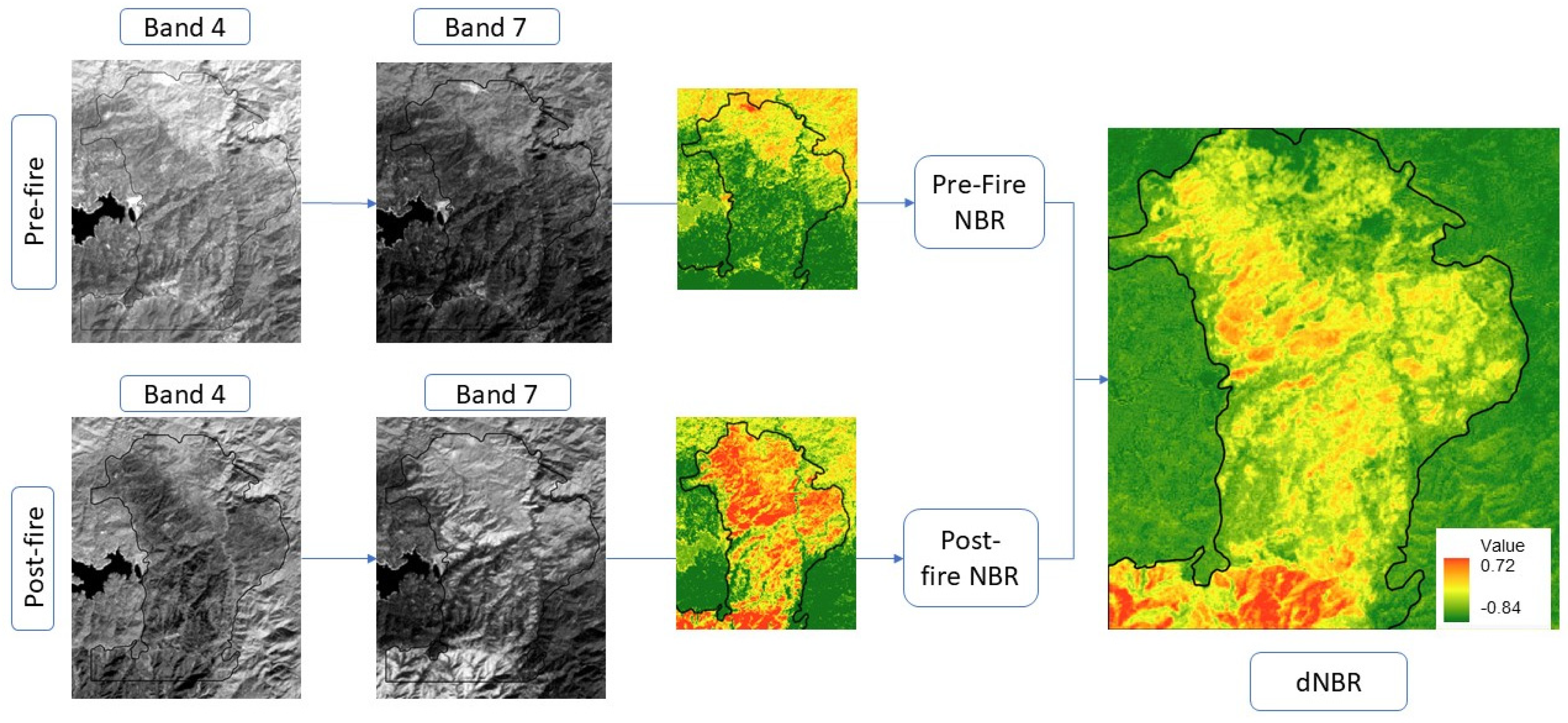
NBR was calculated based on Equation (1) for both pre-fire and post-fire images and was used to calculate dNBR (Equation (2)). dNBR values were classified into unburned, low severity, moderate severity, moderate-high severity, and high severity classes established by Key and Benson (2005) using a threshold-based classifier [18]. The process is shown in Figure 3.
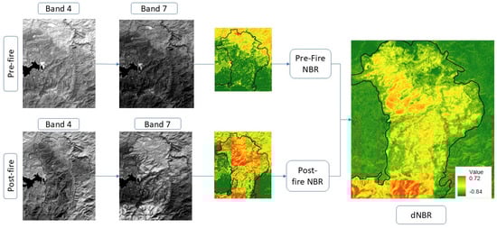
Figure 3.
Burn severity calculation from pre- and post-fire delta normalized burn ratio using NIR (band 4) and SWIR (band 7) bands from Landsat 5 satellite imagery.
2.6. Analytical Methods
The distribution of dead tree density in the study area was analyzed and compared with fire intensity and burn severity distributions. Spatial analyses were conducted based on 21 m × 21 m and 90 m × 90 m grid cells as analytical units, within the domain for which dead trees were mapped. The densities of dead trees within each grid cell were computed using the ‘summary within’ tool provided in ArcGIS toolbox. The zonal statistics tool within the ArcGIS toolbox was used to conduct the averaging and pixel value extraction of the fire intensity variable. We generated two tables of post-fire burn severity measurements including dNBR values and brightness temperature values for each grid size. The tables were joined with the tables consisting of the number of pre-fire dead trees within each grid for both sizes of grids, which resulted in a table consisting of all three elements, number of dead trees, burn severity, and fire intensity, for further comparison. The 21 m grids were used to assess the co-variability of fire intensity and dead trees, and 90 m grids were used for the comparison between burn severity and dead trees.
From the resultant grids with dead tree densities, 111 samples from 90 m grid cells and 113 samples from 21 m grid cells for each cell size were randomly selected for dead tree vs. burn severity and fire intensity analysis. To compile the sample data, we generated random points and extracted the grid values associated with the points in ArcGIS Pro. Sample selections were guided by a minimum distance from other sample cells to minimize the effects of spatial autocorrelation. The minimum distance was established by taking the mapped area and dividing it by the number of samples and then taking the square root to estimate an appropriate separation distance between the samples. For the dead tree vs. fire intensity analysis, a smaller sample size was necessary because the domain of analysis was limited to the zones of active flame front during the FireMapper imaging. The sample separation distance was necessarily smaller to enable a sufficient sample size to be selected for statistical analysis. A separation distance of 500 m was used for sampling the 90 m grid cells while 100 m was used for the sampling of 21 m grid cells. For the TIR pixel values, a threshold of ≥4200 (>63 °C) was selected, which eliminated the comparatively cooler pixels and kept the ones that were hotter and burning during the fire. We assessed the relationship between pre-fire tree mortality and fire intensity as well as burn severity using linear regression in RStudio version 2024.12.1+563 where fire intensity or burn severity were the response variables and tree mortality was the predictor. From this analysis, we generated scatterplots, least square line, regression coefficient, p-value, and f-statistics to determine whether the variables were significantly correlated and, if so, the strength of correlation.
3. Results
3.1. Dead and Live Tree Distributions
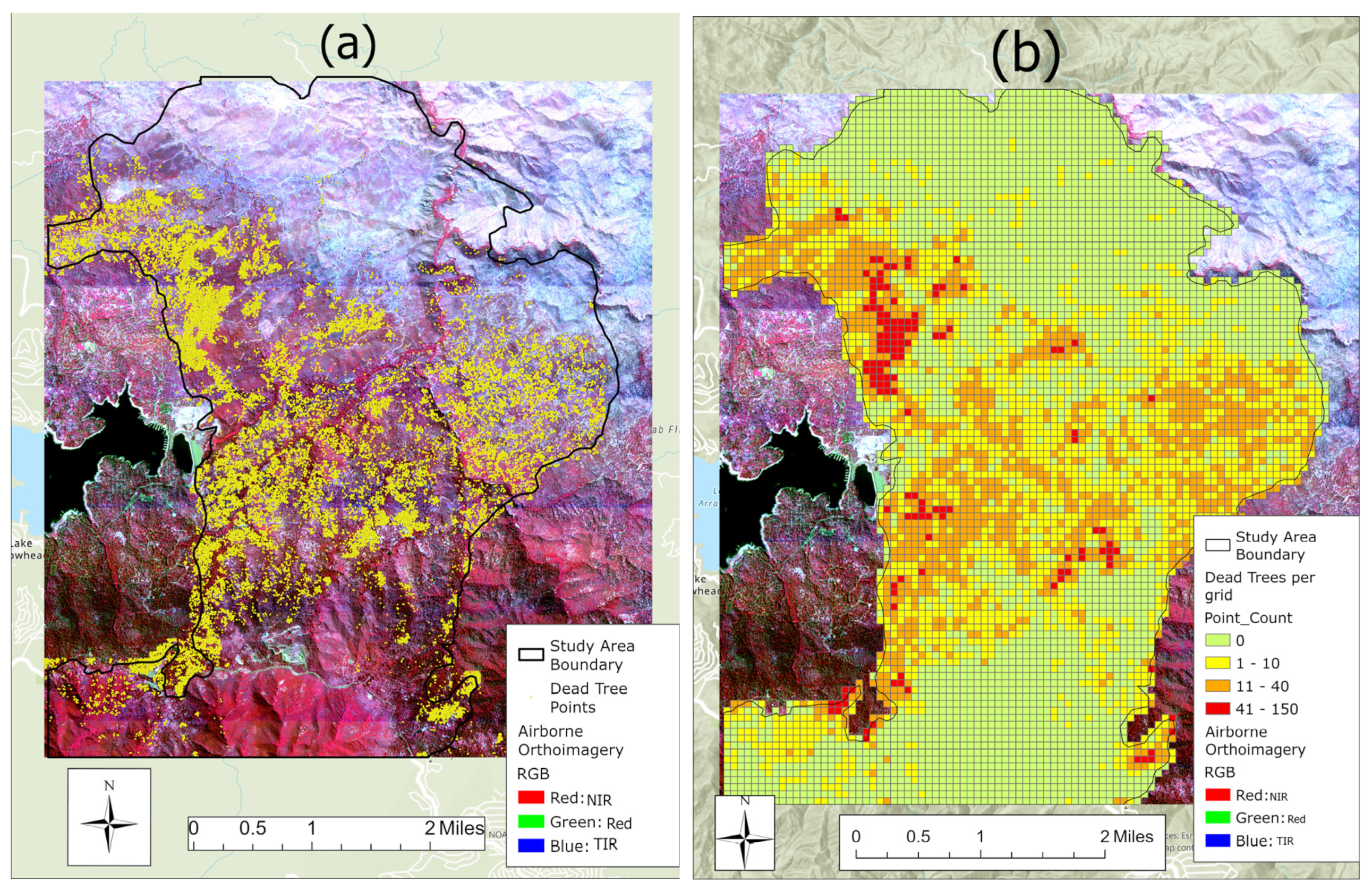
Dead trees were prevalent throughout the San Bernardino Mountains study area prior to the Old Fire, as shown in Figure 4a. The study domain covers an area of 4517 ha and was tessellated by 5795 90 m × 90 m grid cells to summarize tree densities. The dead tree density map shows a denser distribution toward the northwestern part of the study area. A total of 38,258 dead trees were mapped throughout the entire study area. The highest number of dead trees present in a 90 m × 90 m grid cell was 150, or 192 ha−1. Forty-three percent of the samples had no dead trees.

Figure 4.
Distribution of dead trees within the San Bernardino Mountains study area. (a) Presence of pre-fire standing dead trees in yellow portrayed as point shapefile and overlaid on a false-color CIR orthoimage. (b) Density map of pre-fire dead trees for 90 m square grid cells restricted from within the Old Fire burn perimeter.
The study area was also tessellated using a 21 × 21 m grid as the sampling unit incorporating nine (3 × 3) 7 m spatial resolution ATIR pixels. The study domain with eligible ATIR pixels (pixel value ≥ 4200) covered an area of 461 ha covered by 10,454 21 m × 21 m grid cells. The highest number of dead trees present in a 21 m × 21 m grid cell was 14.
A map of dead tree density shows the density distribution throughout the study area in 90 m grids in Figure 4b. The map depicts tree density in four naturally distributed groups with the highest (>40) number of dead trees located in the northwestern part (16–40 trees) and eastern parts of the study area. The non-vegetated northeastern part and vegetated southern part of the study site exhibit the lowest numbers of dead trees (0–1 trees per grid); both areas have relatively lower elevations.
Live trees were mapped for a random sample of grid cells, with 2915 live trees being recorded in the study area. The highest number of live trees recorded for a 90 m × 90 m grid cell was 84 or 108 ha−1 and for a 21 m × 21 m grid cell, the highest number was 8. Thirteen percent of the sample grids had no live trees.
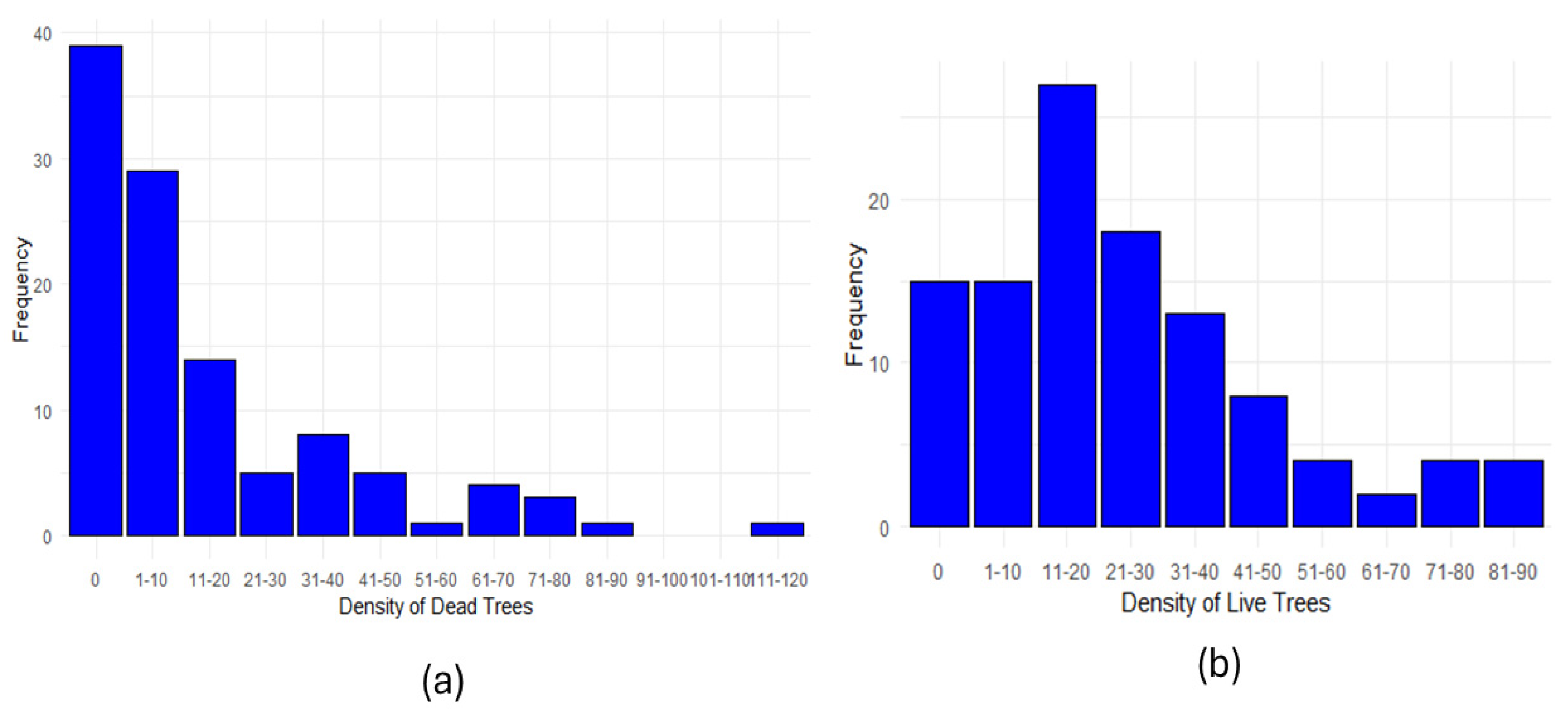
Histograms of the sampled dead and live trees are illustrated in Figure 5. The histogram for live trees was derived from a sample of the 90 m × 90 m grids, while the dead tree histogram is based on the entire study area. A majority of the samples had no or very few dead trees. Most of the sample grids contained 11–20 live trees. The left-skewed histogram curves illustrate a few numbers of live and dead trees for most grid cells.

Figure 5.
Histograms of the frequency distribution of different densities of (a) dead and (b) live trees for the 90 m square grids. The first histogram bin represents grids with no dead or live trees, with the other bins depicting increments of 10 trees per grid cell. Here, n = 111.
3.2. Fire Intensity and Tree Densities
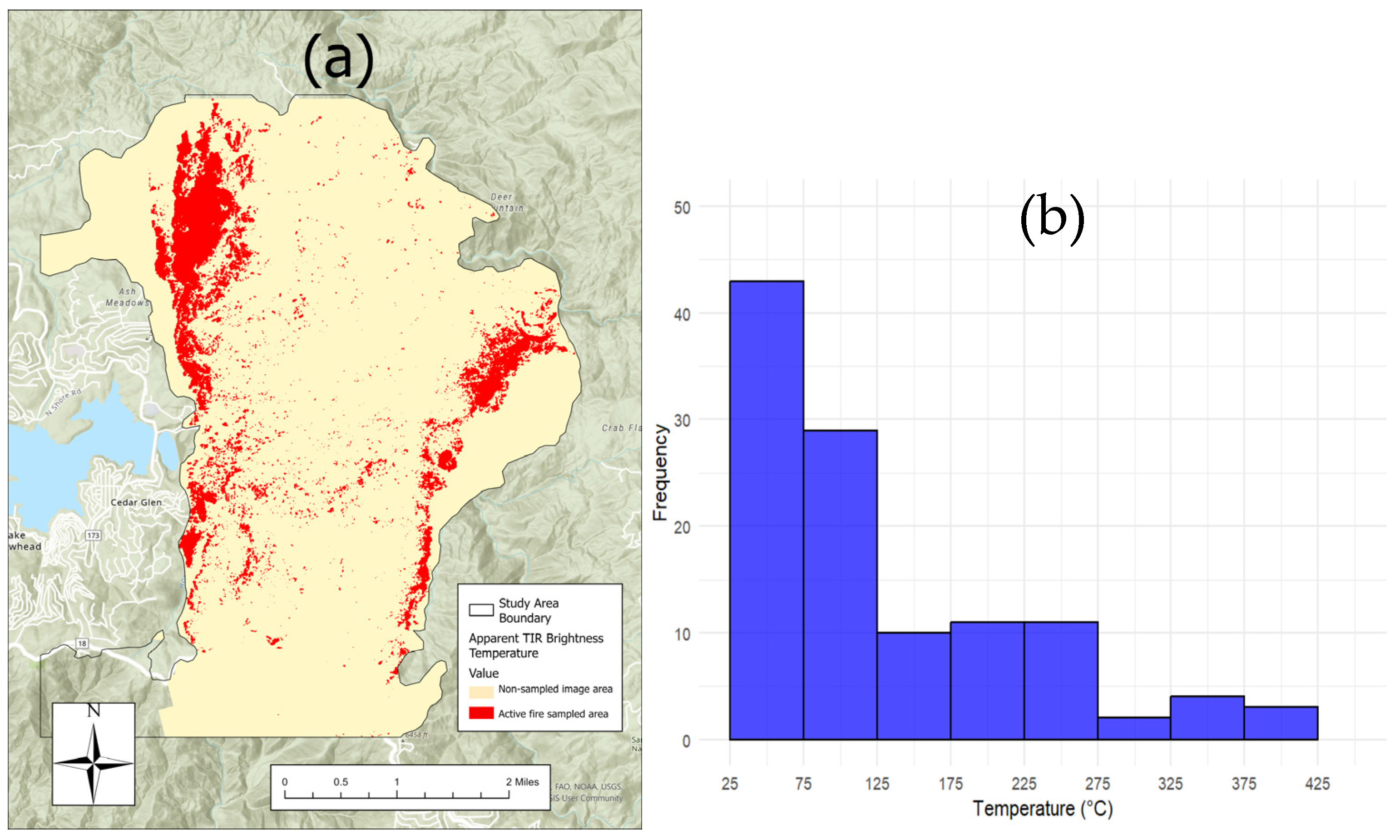
The map in Figure 6a illustrates areas that were actively burning during the FireMapper flights over the Old Fire. Apparent TIR brightness temperatures presented as digital number values ranging from 1 to 8577 were recorded throughout the overpass period. A limited portion of the study area that met the criterion of having a brightness temperature value ≥ 4200 (>63 °C), and therefore considered to have been actively burning at the time of the ATIR overpass, was utilized for the analysis of dead tree count vs. brightness temperature (i.e., fire intensity). Pixels with DN values ≥4200 (>63 °C) are symbolized by red color on the map, indicating potential sampling areas inside the Old Fire perimeter for assessing apparent brightness temperature vs. tree density relationships. Figure 6b shows a histogram of the distribution of apparent brightness temperatures across different intervals from the 113 samples of 21 m × 21 m grids. The sampled apparent TIR brightness temperature ranges from 4200 (~63 °C) up to 5600 (425 °C) digital number value, with a majority of the pixels in the 4200–4300 (63–113 °C) range.

Figure 6.
(a) Map of locations where TIR brightness temperatures were ≥ 4200 (>63 °C). (b) Histogram of temperature in degree C reveals that more than half (63) of the 113 random samples were selected from the lower end of TIR values. n = 113.
The left-skewed histogram in Figure 6b reveals that the majority of the apparent TIR brightness temperatures in the sampled grids fall in the lower end of the active fire temperature range.
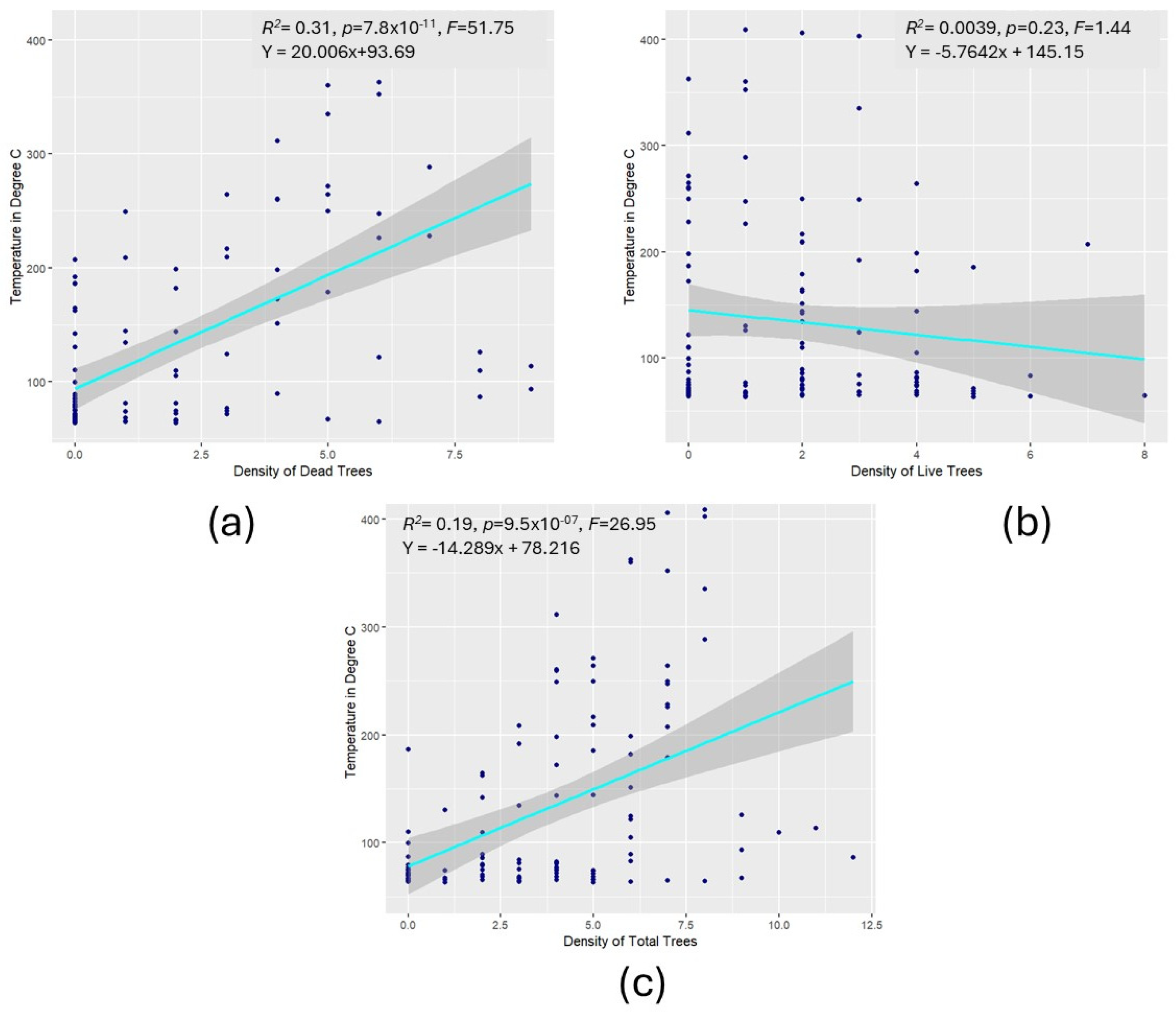
The relationships of apparent TIR brightness temperature with pre-fire dead, live, and total trees were tested. Linear regression results are depicted in Figure 7. Results show a significant relationship with moderate co-variability between apparent TIR brightness temperature and pre-fire dead tree density (R2 = 0.31, p < 0.01, n = 113). They also show a significant relationship but weaker co-variability with total trees (R2 = 0.19, p < 0.01, n = 113). However, apparent TIR brightness temperature’s relationship to live tree density is not significant. A p-value < 0.05 is considered significant and is highlighted in bold in the table. Figure 7 shows the scatterplots and linear regression with a best-fit regression line symbolized in cyan. Both the dead tree (Figure 7a) and total tree (Figure 7c) density scatterplots have a positive linear relationship with fire intensity, while the live tree (Figure 7b) scatterplot shows no apparent trend.
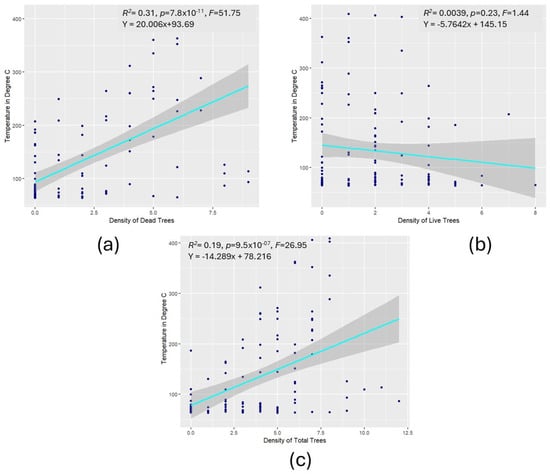
Figure 7.
Scatterplot and linear regression results for temperature in degree C (ATIR brightness temperature ≥ 4200 or >63 °C) vs. (a) dead tree, (b) live tree, and (c) total tree density. n = 113.
3.3. Burn Severity and Tree Densities
The burn severity map derived from Landsat 5 dNBR with a pre-fire dead trees map overlayed is shown in Figure 8a. dNBR values ranged from −0.15 to +0.66, with lower values representing less severe burn presented in green and higher values representing severe burn shown in red. Upon visual inspection, it appears that the areas with higher burn severity correspond spatially with the denser distribution of pre-fire dead trees. However, in contrast, on the southern portion of the study area, grids with higher dNBR values were observed to have no dead trees.
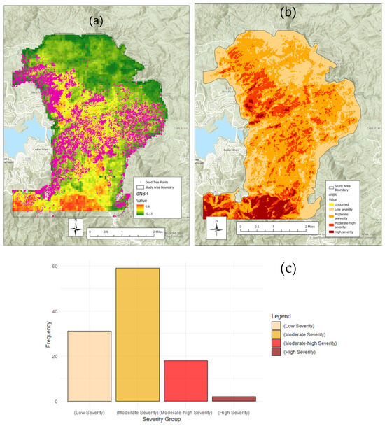
Figure 8.
(a) Pre-fire dead trees overlayed on a Landsat 5 dNBR map. (b) Burn severity map with five burn categories adapted from Key and Benson (2006). (c) Histogram shows the distribution of 111 random samples from the dNBR value ranges.
Figure 8b shows the burn severity map classified into five categories: unburned, low severity, moderate severity, moderate-high severity, and high severity following Key and Benson (2006). Areas having moderate-high severe and high severe burn commonly coincide with areas having higher densities of dead trees. A dNBR value histogram is presented in Figure 8c which shows the frequency of each burn category. The most common burn category was the moderate-severity burn category, while no unburned area was present within the study area.
The linear regression results (Figure 9) show a weak but significant relationship of dNBR with the distribution of pre-fire dead tree (R2 = 0.14, p < 0.01, n = 111) and total tree (R2 = 0.18, p < 0.01, n = 111) density and no significant relationship with live tree (p > 0.05) density. Like the TIR scatterplots, a p- value < 0.05 is considered significant and is highlighted in bold in the table.
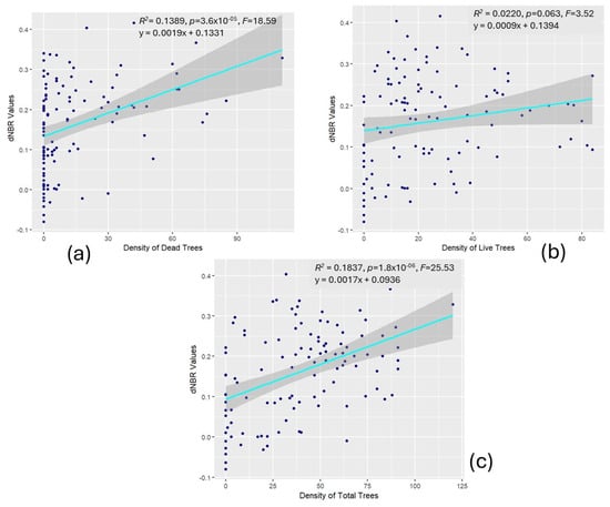
Figure 9.
Linear regression: burn severity vs. (a) dead trees, (b) live trees, and (c) total trees.
Figure 9 shows scatterplots and linear regression with a best-fit regression line symbolized in cyan. Figure 9a,c are relationships of burn severity with pre-fire dead and total trees which shows a positive trend line. The horizontal line in Figure 9b suggests that no significant relationship is present.
4. Discussion
A substantial number of pre-fire dead trees were mapped in the study area, and they were moderately and weakly co-related with fire intensity and burn severity, respectively. We addressed one of the research questions of this study that pertains to the distribution of pre-fire dead trees in the Old Fire perimeter in San Bernardino Mountains. We also addressed research questions pertaining to the relationship of pre-fire dead trees with apparent TIR brightness temperature and post-fire burn severity. Findings of the statistical analysis elucidate that there is a significant relationship of pre-fire dead trees with fire intensity and a weak but significant relationship with burn severity.
4.1. Distribution of Dead and Live Trees
Pre-fire dead trees mapped using very-high-spatial-resolution (1.6 m) airborne imagery were found to be distributed throughout much of the study area. Tree mortality is attributed to drought and bark beetle infestation in the forest, killing thousands of conifer trees as well as chaparral shrubs [11]. Bark beetles may attack suitable host trees in proximity of few hundred meters [28]. This supports the findings that clusters of higher-density dead trees were located within hundreds of meters from each other. A study by Freeman et al. (2017) reported tree mortality in montane mixed conifer forests in San Diego County due to drought and beetle infestation [29]. Freeman et al. (2017) reported tree mortality occurring in clusters, with peak mortality occurring between 2002 and 2005, which supports our findings that large numbers of dead trees existed in the San Bernardino Mountains during 2003. However, the number of dead trees per hectare estimated in the Freeman et al. (2017) study was much lower than our findings [29]. The highest number of dead trees found was 10.3 dead trees per ha in 2005 for Palomar Mountain, compared to a maximum of 192 dead trees per ha in our study. This could also be an outcome of the substantial effort to remove dead trees on Palomar Mountain from 2003–2005 [29].
The majority of the grid cells within our study area prior to the Old Fire had no dead trees. Dead trees were predominantly present in the northwestern part of the study area, located east of Lake Arrowhead. The cells with the highest number of dead trees recorded were also located in this portion of the study area. Five of the grid cells had over one hundred dead trees.
Bond et al. (2009) assessed the distribution of dead trees in the Old Fire and Grand Prix Fire perimeter in 2003 (a much larger areal extent than our study site), with 22 dead trees per ha reported as the maximum, which is substantially lower than our findings of 192 dead trees per ha [12]. Fifty percent of their study area was found to have no dead trees, which was slightly higher than 43% grid cells for our study.
Live tree density in our study was only estimated for a sample of grid cells in the study area for both 90 m and 21 m grids; the highest number of live trees found per hectare was 108. Freeman et al. (2017) also mapped and analyzed the distribution of live trees per hectare, which ranged from 99 to 273 live trees per ha. We found a weak but significant negative correlation between the numbers of dead and live trees for each grid cell, indicating that areas with higher numbers of dead trees tended to have lower numbers of live trees. This is similar to the findings of Freeman et al. (2017) for the Palomar and Volcan mountains.
The deep learning routine and multispectral imagery used in this study yielded poor estimates of dead tree density, primarily due to the mismatch in image resolution and the deep learning algorithm. Generally, deep learning models built with the ArcGIS Pro are reported to yield accurate tree mapping results for imagery having spatial resolutions of 10–25 cm; the airborne image used in our study has a spatial resolution of 1.6 m. Detected trees from the deep learning model had several false-positive and false-negative detections; despite that, 7501 out of the 38,258 dead trees were correctly detected by the model.
4.2. Influence of Dead Trees on Fire Intensity
The Old Fire started on 25th October, but the ATIR images utilized in this study were taken four days after the fire started. The fire spread was captured by four different imaging passes throughout the day; the active front was moving to the west and north, in a similar location to most of the recorded dead trees for the 21 m sample grids. Although the imaging repeat frequency was low, the four passes enabled the direction of fire spread to be discerned, which was moving in the direction of the Santa Ana winds, to the west. A significant correlation was found between apparent brightness temperature (as a metric for fire intensity) and dead trees with R2 = 0.31, which means that 31% of the variance in fire intensity can be explained by dead tree density. However, other factors such as topography and wind speed and direction likely influenced the fire intensity as well, which were not addressed in this study. A study in the Sierra Nevada Mountains by Stephens et al. (2022) concluded similarly that pre-fire dead and live tree densities influenced fire intensity [3]. The tree mortality noted by Stephens et al. (2022) also resulted from drought and beetle infestation effects. The study identified the combination of dead and live tree density as a key influence for increasing fire intensity [3]. Although we found no significant correlation between fire intensity (brightness temperature) and live trees, a moderate significant correlation (R2 = 0.19) was found between fire intensity and total trees, which is the sum of dead and live trees in a grid cell. Dead and dry fuel are highly flammable and contribute to the severity of fire [8]. The lack of water content in dead vegetation makes them highly combustible. The dead fuel combustion then contributes to faster drying out of living foliage as well, increasing fire intensity as a whole [30]. The age of the dead fuel can also influence the fire intensity, as older fuel can increase fire intensity [31]. However, much of the drought- and beetle-caused tree mortality occurred just prior to the fire of 2003. Specifically between 2001 and 2004, drought-weakened trees in southern California were susceptible to different species of bark beetle infestation. Mortality in early years contributes to catastrophic wildfires including crown fires.
The relatively high-spatial-resolution TIR imagery used in this research was a composite of four flight passes from different times of the same day. Visual observations on some of the samples containing a higher number of dead trees (8–9 dead trees per sample) showed lower apparent TIR brightness temperature values. This could be a result of the fire already passing through the sampled points when the images were acquired.
4.3. Influence of Dead Trees on Burn Severity
From the linear regression results, the spatial association of burn severity with the pre-fire dead and total trees is found to be moderately significant with R2 values of 0.14 and 0.18, respectively. The correlation is weak, likely because the pre-fire dead and total tree density are not the only factors influencing the burn severity of the fire, but other factors such as topography, fuel characteristics, wind direction, etc. were also present. Moreover, dNBR is an image-derived surrogate for actual burn severity.
Contrary to our findings, Bond et al. (2009) found no evidence of the drought- and pine beetle-caused tree mortality influencing the fire severity of the Old and Grand Prix fires [12]. They used Landsat TM RdNBR data for the burn severity analysis and studied the entire burned area within the perimeter of both wildfires and divided the burn severity into four categories. However, they found no correlation (p = 0.88) between the pre-fire dead trees and moderate-severe burned areas. The number of dead trees per ha noted in the Bond et al. (2009) study was much lower than what we observed [12]. However, their estimates were based on visual estimates from aircraft overflights conducted by the USDA Forest Service, whereas we directly mapped dead tree locations using high-resolution (1.6 m) airborne imagery. Our different study area extents (entire Old and Grand Prix fire perimeter) are another likely explanation for the contrasting results.
5. Conclusions
A major contribution of this study is the generation and analysis of detailed pre-fire dead tree maps, made possible from acquired airborne multispectral orthoimagery captured and processed by the USDA Forest Service Pacific Southwest Research Station. This enabled the spatial representation of densities of dead trees throughout the study area. A major finding of the study is that pre-fire dead trees significantly covary with the fire intensity (R2 = 0.31) and burn severity (R2 = 0.14).
This study provides insights in understanding the gap in the relationship between pre-fire dead trees and fire intensity and burn severity. The key contributing factors of this research are threefold: (1) generating an effective methodology for accurately mapping the spatial distribution of pre-fire dead trees using high-spatial-resolution (1.6 m) multispectral imagery and (2) conducting statistical analyses to reveal the underlying spatial association of pre-fire dead trees with ATIR-derived fire intensity and (3) Landsat 5-derived post-fire burn severity. Although previous studies have evaluated factors affecting fire behavior, this study focuses on the pre-existing dead and live trees. Statistical analysis supports the hypothesis that pre-fire dead trees had a significant influence on the fire intensity and post-fire burn severity for the Old Fire. This study is useful for understanding fire behavior and providing important information to policymakers and land managers for future fire prevention and management.
Author Contributions
Conceptualization, D.A.S. and P.R.; Methodology, N.N.; Software, N.N.; Formal analysis, N.N.; Resources, D.A.S., P.R. and D.S.; Data curation, N.N., R.T. and L.W.; Writing—original draft, N.N.; Writing—review & editing, D.A.S., P.R., D.S. and M.K.J.; Supervision, D.A.S., P.R. and D.S.; Funding acquisition, P.R. and D.S. All authors have read and agreed to the published version of the manuscript.
Funding
Funding to support this research was provided by the USDA Forest Service, Pacific Southwest Research Station grants: G00012222 (Effects of Drought Stress and Forest Management on Fire Behavior and Post-Fire Forest Structure in Western Coniferous Forest) and grant G000147000 (Remote Sensing of Forest Health and Fire Effects). Ms. Nawar received support from the SDSU McFarland Geography Scholarship and the SDSU Division of Research and Innovation through the Grants for Established RSCA program through “Graduate Student Support for NASA FireSense Implementation Team”. D.S. gratefully acknowledges funding from the NASA FireSense airborne science program (Grant # 80NSSC24K0145 and 80NSSC24K1320), the NASA FireSense Implementation Team (Grant # 80NSSC24K1320), the NASA EMIT Science and Applications Team (Grant # 80NSSC24K0861), the USDA NIFA Sustainable Agroecosystems program (Grant #2022-67019-36397), the USDA AFRI Rapid Response to Extreme Weather Events Across Food and Agricultural Systems program (Grant #2023-68016-40683), the NASA Land-Cover/Land Use Change program (Grant #NNH21ZDA001N-LCLUC), the NASA Remote Sensing of Water Quality program (Grant #80NSSC22K0907), the NASA Applications-Oriented Augmentations for Research and Analysis Program (Grant #80NSSC23K1460), the NASA Commercial Smallsat Data Analysis Program (Grant #80NSSC24K0052), the California Climate Action Seed Award Program, and the NSF Signals in the Soil program (Award #2226649).
Institutional Review Board Statement
Not applicable.
Informed Consent Statement
Not applicable.
Data Availability Statement
The original contributions presented in the study are included in the article, further inquiries can be directed to the corresponding author.
Conflicts of Interest
The authors declare no conflict of interest.
References
- Everett, R.G. Dendrochronology-based fire history of mixed-conifer forests in the San Jacinto Mountains, California. For. Ecol. Manag. 2008, 256, 1805–1814. [Google Scholar] [CrossRef]
- Reed, C.C.; Hood, S.M. Few generalizable patterns of tree-level mortality during extreme drought and concurrent bark beetle outbreaks. Sci. Total Environ. 2021, 750, 141306. [Google Scholar] [CrossRef] [PubMed]
- Stephens, S.L.; Bernal, A.A.; Collins, B.M.; Finney, M.A.; Lautenberger, C.; Saah, D. Mass fire behavior created by extensive tree mortality and high tree density not predicted by operational fire behavior models in the southern Sierra Nevada. For. Ecol. Manag. 2022, 518, 120258. [Google Scholar] [CrossRef]
- Stuart, J.D.; Agee, J.K.; Gara, R.I. Lodgepole pine regeneration in an old, self-perpetuating forest in south central Oregon. Can. J. For. Res. 1989, 19, 1096–1104. [Google Scholar] [CrossRef]
- Keeley, J.E.; Zedler, P.H. Large, high-intensity fire events in southern California shrublands: Debunking the fine-grain age patch model. Ecol. Appl. 2009, 19, 69–94. [Google Scholar] [CrossRef]
- Petropoulos, G.P.; Islam, T. (Eds.) Remote Sensing of Hydrometeorological Hazards, 1st ed.; CRC Press: Boca Raton, FL, USA, 2018; Taylor & Francis: Abingdon, UK, 2017; ISBN 978-1-315-15494-7. [Google Scholar]
- Keeley, J.E. Fire intensity, fire severity and burn severity: A brief review and suggested usage. Int. J. Wildland Fire 2009, 18, 116. [Google Scholar] [CrossRef]
- Keeley, J.E.; Syphard, A.D.; Fotheringham, C.J. The 2003 and 2007 Wildfires in Southern California. In Natural Disasters and Adaptation to Climate Change; Boulter, S., Palutikof, J., Karoly, D.J., Guitart, D., Eds.; Cambridge University Press: Cambridge, UK, 2013; pp. 42–52. ISBN 978-0-511-84571-0. [Google Scholar]
- Syphard, A.D.; Keeley, J.E. Location, timing and extent of wildfire vary by cause of ignition. Int. J. Wildland Fire 2015, 24, 37. [Google Scholar] [CrossRef]
- Fellows, A.W.; Goulden, M.L. Rapid vegetation redistribution in Southern California during the early 2000s drought. J. Geophys. Res. Biogeosci. 2012, 117, 1–11. [Google Scholar] [CrossRef]
- Riggan, P.J.; Tissell, R.G. Chapter 6 Airborne Remote Sensing of Wildland Fires. In Developments in Environmental Science; Elsevier: Amsterdam, The Netherlands, 2008; Volume 8, pp. 139–168. ISBN 978-0-08-055609-3. [Google Scholar]
- Bond, M.L.; Lee, D.E.; Bradley, C.M.; Hanson, C.T. Influence of Pre-Fire Tree Mortality on Fire Severity in Conifer Forests of the San Bernardino Mountains, California. Open For. Sci. J. 2009, 2, 41–47. [Google Scholar] [CrossRef]
- Chu, T.; Guo, X. Remote Sensing Techniques in Monitoring Post-Fire Effects and Patterns of Forest Recovery in Boreal Forest Regions: A Review. Remote Sens. 2014, 6, 470–520. [Google Scholar] [CrossRef]
- Hirschmugl, M.; Ofner, M.; Raggam, J.; Schardt, M. Single tree detection in very high resolution remote sensing data. Remote Sens. Environ. 2007, 110, 533–544. [Google Scholar] [CrossRef]
- Chen, Y.; Morton, D.C.; Randerson, J.T. Remote sensing for wildfire monitoring: Insights into burned area, emissions, and fire dynamics. One Earth 2024, 7, 1022–1028. [Google Scholar] [CrossRef]
- Johnston, J.M.; Wooster, M.J.; Paugam, R.; Wang, X.; Lynham, T.J.; Johnston, L.M. Direct estimation of Byram’s fire intensity from infrared remote sensing imagery. Int. J. Wildland Fire 2017, 26, 668. [Google Scholar] [CrossRef]
- Cocke, A.E.; Fulé, P.Z.; Crouse, J.E. Comparison of burn severity assessments using Differenced Normalized Burn Ratio and ground data. Int. J. Wildland Fire 2005, 14, 189. [Google Scholar] [CrossRef]
- Key, C.H.; Benson, N.C. Landscape Assessment (LA). In FIREMON: Fire Effects Monitoring and Inventory System. Gen. Tech. Rep. RMRS-GTR-164-CD; Lutes, D.C., Keane, R.E., Caratti, J.F., Key, C.H., Benson, N.C., Sutherland, S., Gangi, L.J., Eds.; Department of Agriculture, Forest Service, Rocky Mountain Research Station: Fort Collins, CO, USA, 2006; Volume 164, p. LA-1-55. [Google Scholar]
- Kinoshita, A.M.; Hogue, T.S. Spatial and temporal controls on post-fire hydrologic recovery in Southern California watersheds. Catena 2011, 87, 240–252. [Google Scholar] [CrossRef]
- Lewis, S.A.; Lentile, L.B.; Hudak, A.T.; Robichaud, P.R.; Morgan, P.; Bobbitt, M.J. Mapping Ground Cover Using Hyperspectral Remote Sensing after the 2003 Simi and Old Wildfires in Southern California. Fire Ecol. 2007, 3, 109–128. [Google Scholar] [CrossRef]
- Jin, Y.; Randerson, J.T.; Faivre, N.; Capps, S.; Hall, A.; Goulden, M.L. Contrasting controls on wildland fires in Southern California during periods with and without Santa Ana winds. J. Geophys. Res. Biogeosci. 2014, 119, 432–450. [Google Scholar] [CrossRef]
- Keeley, J.E.; Fotheringham, C.J.; Moritz, M.A. Lessons from the October 2003. Wildfires in Southern California. J. For. 2004, 102, 26–31. [Google Scholar] [CrossRef]
- Stephenson, J.R.; Calcarone, G.M. Southern California Mountains and Foothills Assessment: Habitat and Species Conservation Issues; U.S. Department of Agriculture, Forest Service, Pacific Southwest Research Station: Albany, CA, USA, 2016; p. PSW-GTR-172.
- Minnich, R.A.; Barbour, M.G.; Burk, J.H.; Fernau, R.F. Sixty Years of Change in Californian Conifer Forests of the San Bernardino Mountains. Conserv. Biol. 1995, 9, 902–914. [Google Scholar] [CrossRef]
- Roman, T. Land Management Plan Monitoring Report for the Angeles, Cleveland, and San Bernardino National Forests (2021–2022); United States Department of Agriculture: Washington, DC, USA, 2022.
- Eidenshink, J.; Schwind, B.; Brewer, K.; Zhu, Z.-L.; Quayle, B.; Howard, S. A Project for Monitoring Trends in Burn Severity. Fire Ecol. 2007, 3, 3–21. [Google Scholar] [CrossRef]
- Miller, J.D.; Thode, A.E. Quantifying burn severity in a heterogeneous landscape with a relative version of the delta Normalized Burn Ratio (dNBR). Remote Sens. Environ. 2007, 109, 66–80. [Google Scholar] [CrossRef]
- Kapil, R.; Marvasti-Zadeh, S.M.; Goodsman, D.; Ray, N.; Erbilgin, N. Classification of Bark Beetle-Induced Forest Tree Mortality using Deep Learning. arXiv 2022. [Google Scholar] [CrossRef]
- Freeman, M.P.; Stow, D.A.; An, L. Patterns of mortality in a montane mixed-conifer forest in San Diego County, California. Ecol. Appl. 2017, 27, 2194–2208. [Google Scholar] [CrossRef] [PubMed]
- Keeley, J.; Fotheringham, C. Impact of Past, Present, and Future Fire Regimes on North American Mediterranean Shrublands. In Ecological Studies; Springer: Berlin/Heidelberg, Germany, 2003; Volume 160, pp. 218–262. ISBN 978-0-387-95455-4. [Google Scholar]
- Riggan, P.; Wolden, L.; Tissell, B.; Weise, D.; Coen, J. Remote Sensing Fire and Fuels in Southern California. In Proceedings of the 3rd Fire Behavior and Fuel Conference, 25–29 October 2010, Spokane, WA, USA; Wade, D.D., Robinson, M.L., Eds.; International Association of Wildland Fire: Birmingham, AL, USA, 2011. 14p. [Google Scholar]


Disclaimer/Publisher’s Note: The statements, opinions and data contained in all publications are solely those of the individual author(s) and contributor(s) and not of MDPI and/or the editor(s). MDPI and/or the editor(s) disclaim responsibility for any injury to people or property resulting from any ideas, methods, instructions or products referred to in the content. |
© 2025 by the authors. Licensee MDPI, Basel, Switzerland. This article is an open access article distributed under the terms and conditions of the Creative Commons Attribution (CC BY) license (https://creativecommons.org/licenses/by/4.0/).