

Optimized Machine Learning Model for Fire Consequence Prediction

Abstract
1. Introduction
2. Methodology
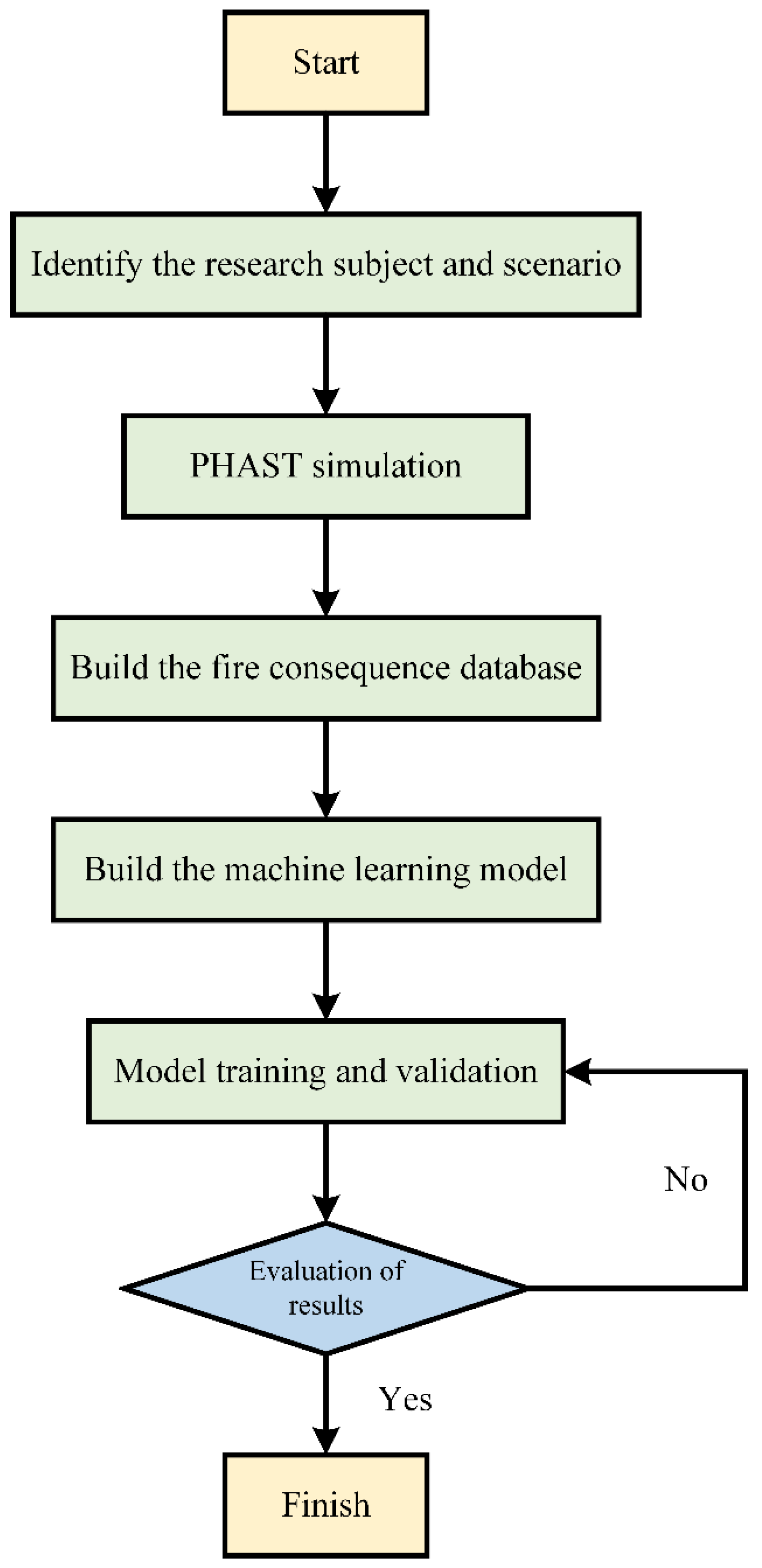
2.1. Workflow of the Model Design
- (1)
- Identify the research subject and scenarios; simulate the consequences of tank leaks and fires using PHAST.
- (2)
- Construct a database of fire consequences based on the simulation results from PHAST.
- (3)
- Develop a quantitative prediction model for the range of consequences based on the database; these include a BP neural network, random forest regression, and K-R regression prediction models.
- (4)
- Tune the prediction models to determine the optimal model.
- (5)
- Evaluate the model’s performance by calculating the mean squared error (MSE) and the R2 coefficient of determination [17].
- (6)
- Apply machine learning algorithms to predict the consequences of fire accidents caused by leaks from storage tanks and draw conclusions by comparing and analyzing actual cases with the predictive results.
2.2. PHAST Model
2.3. Machine Learning
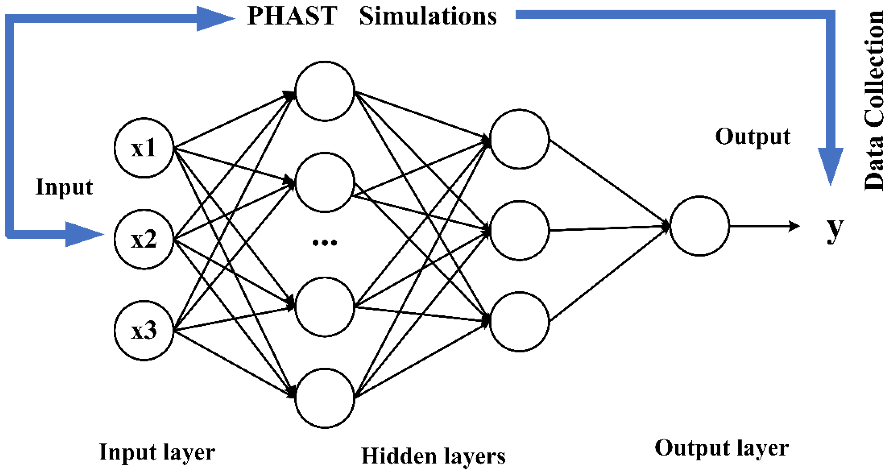
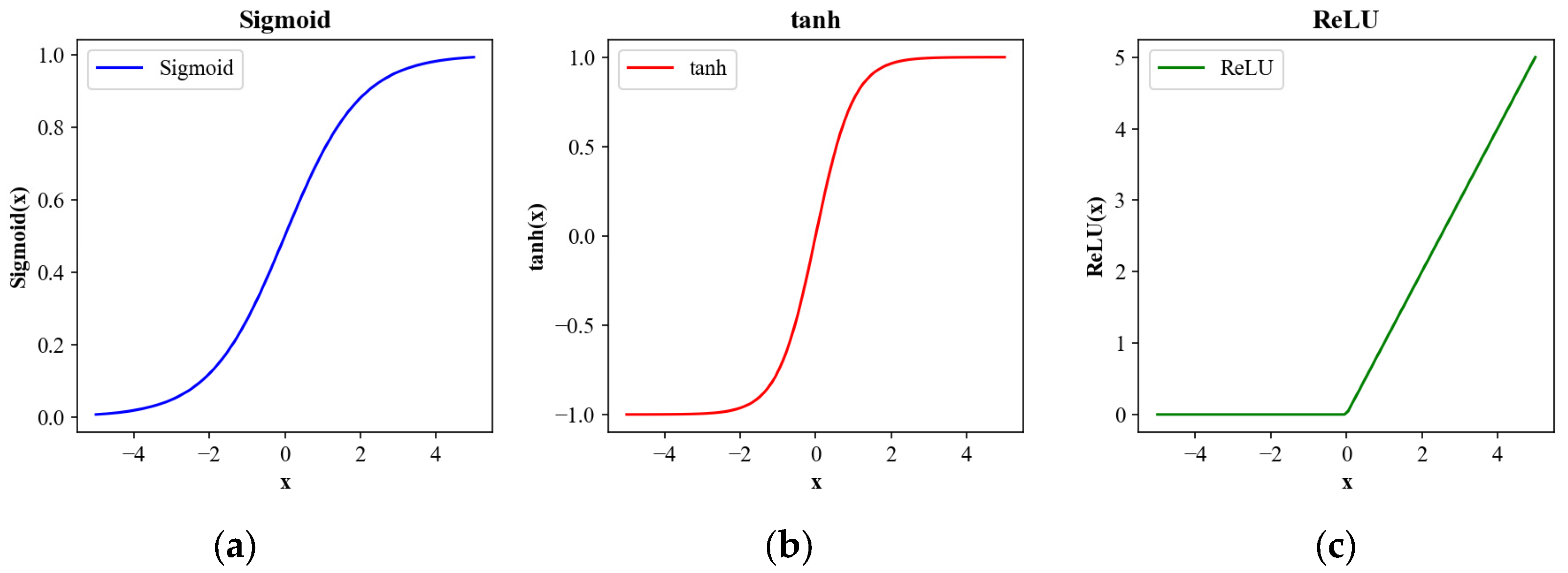
2.3.1. BP Neural Network
2.3.2. Random Forest
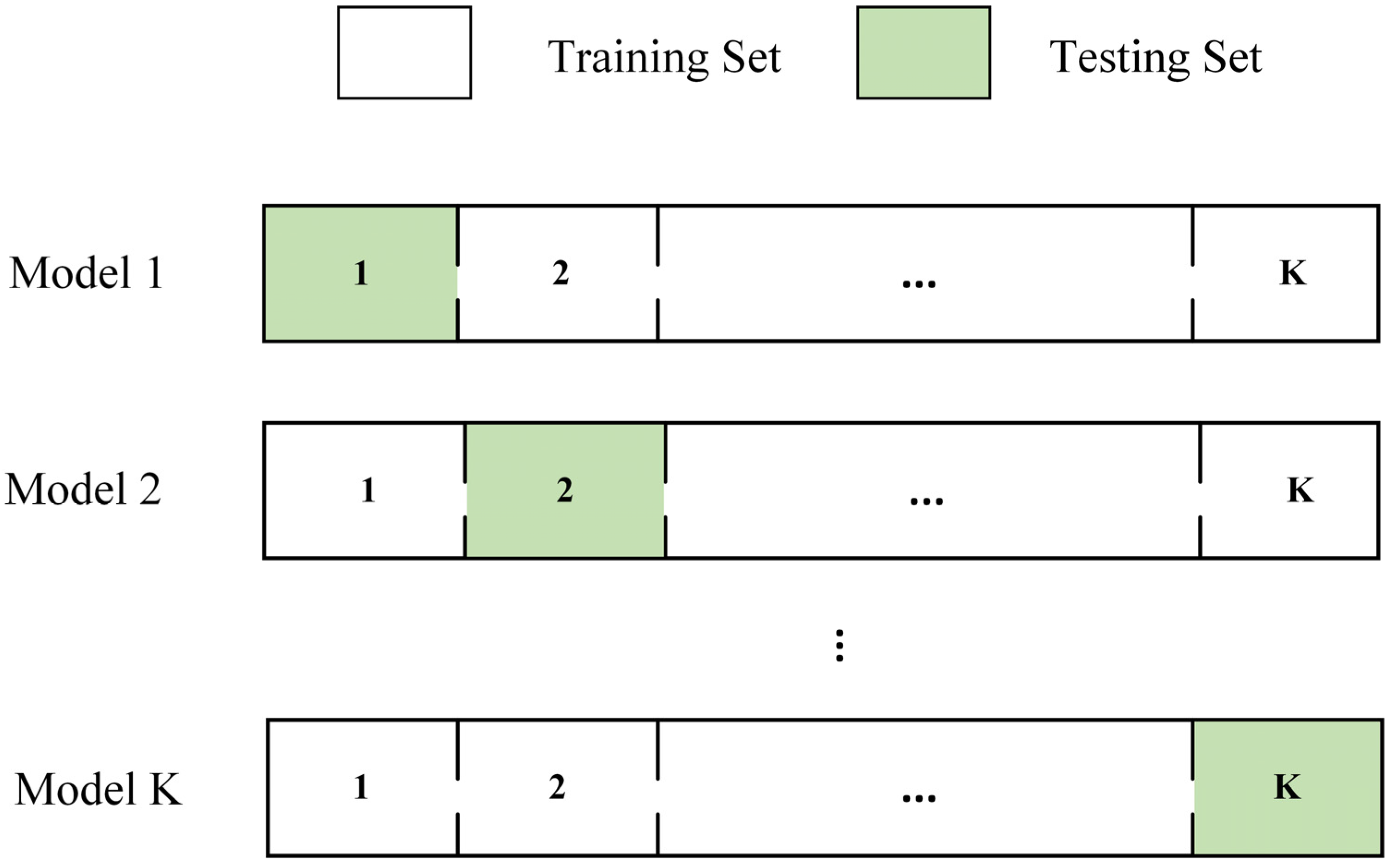
2.3.3. Cross-Validation
2.4. Model Evaluation
3. Data Preprocessing and Discussion
3.1. Data Preprocessing
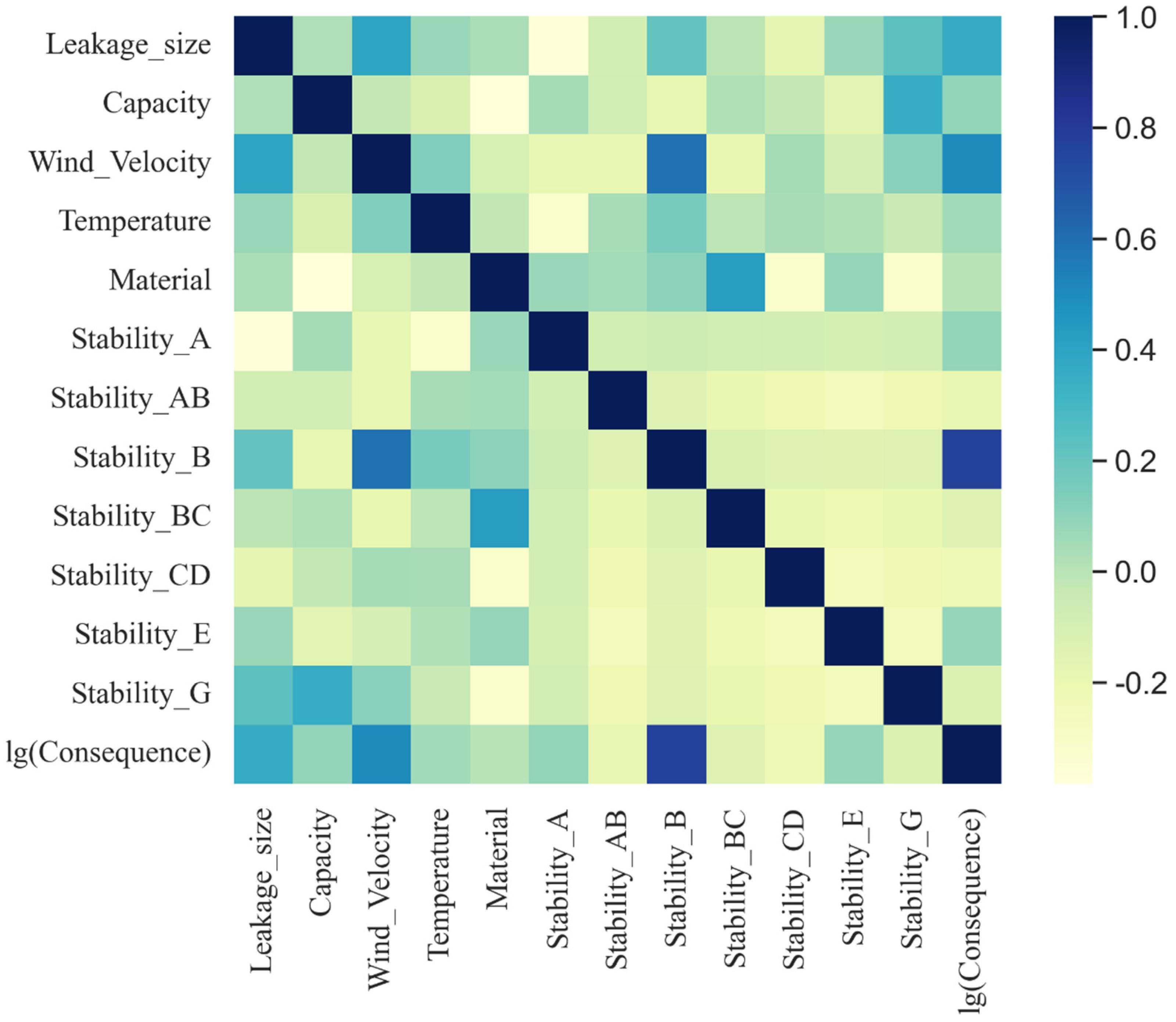
3.1.1. Correlation Analysis
3.1.2. Multicollinearity
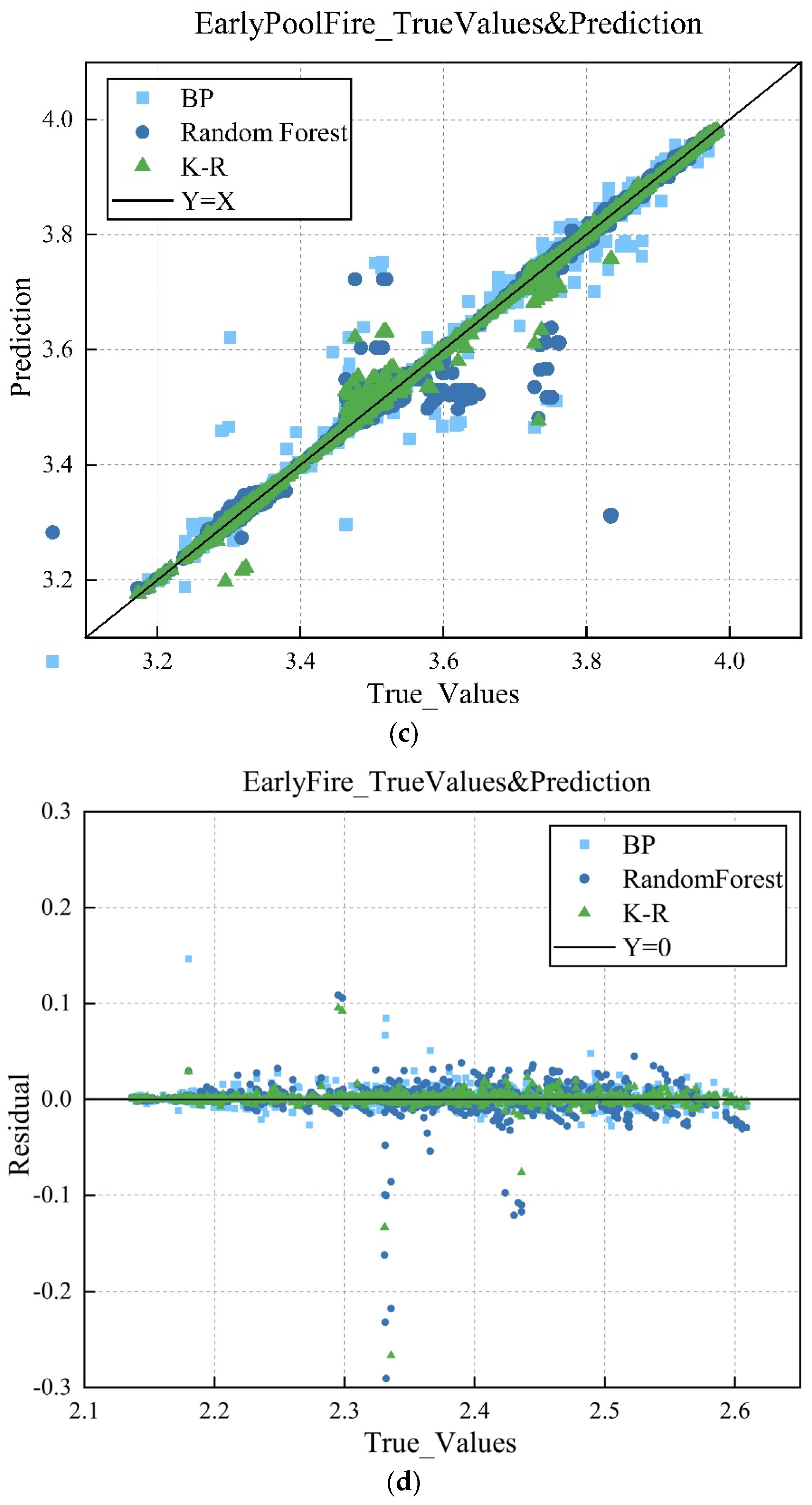
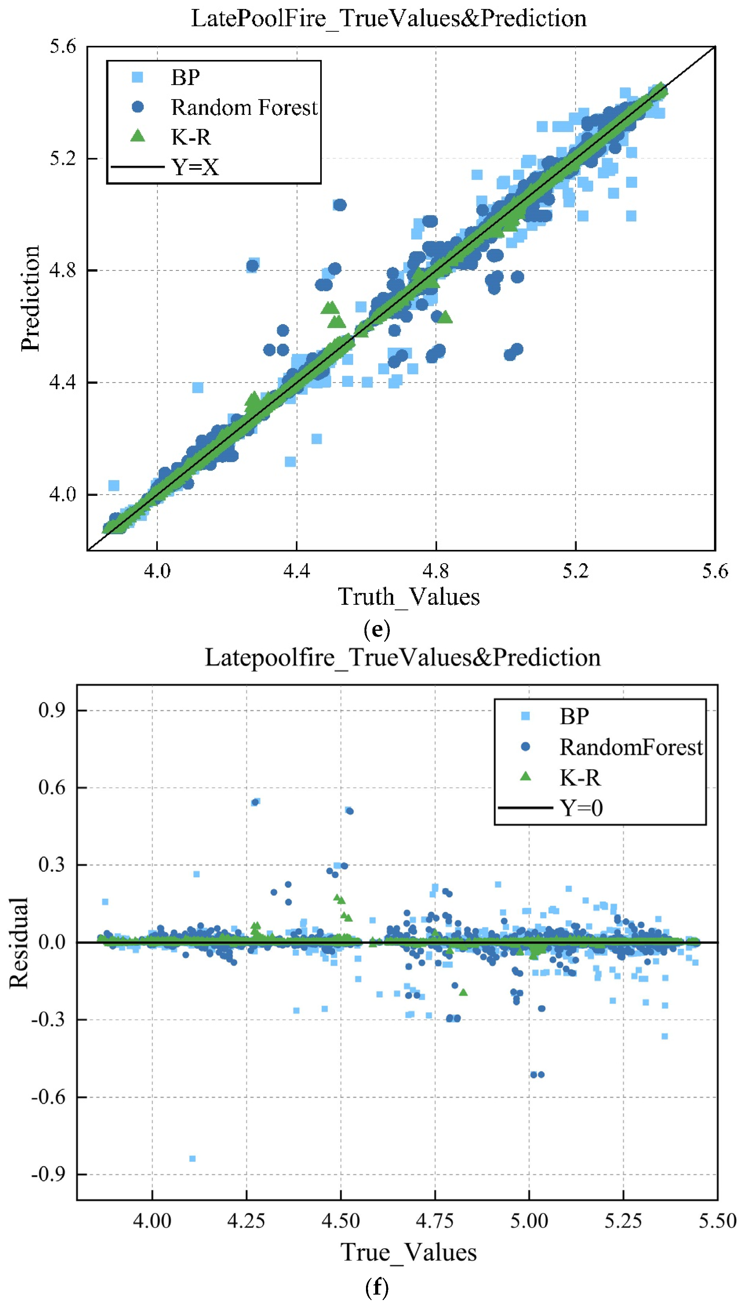
3.2. Discussion
4. Conclusions
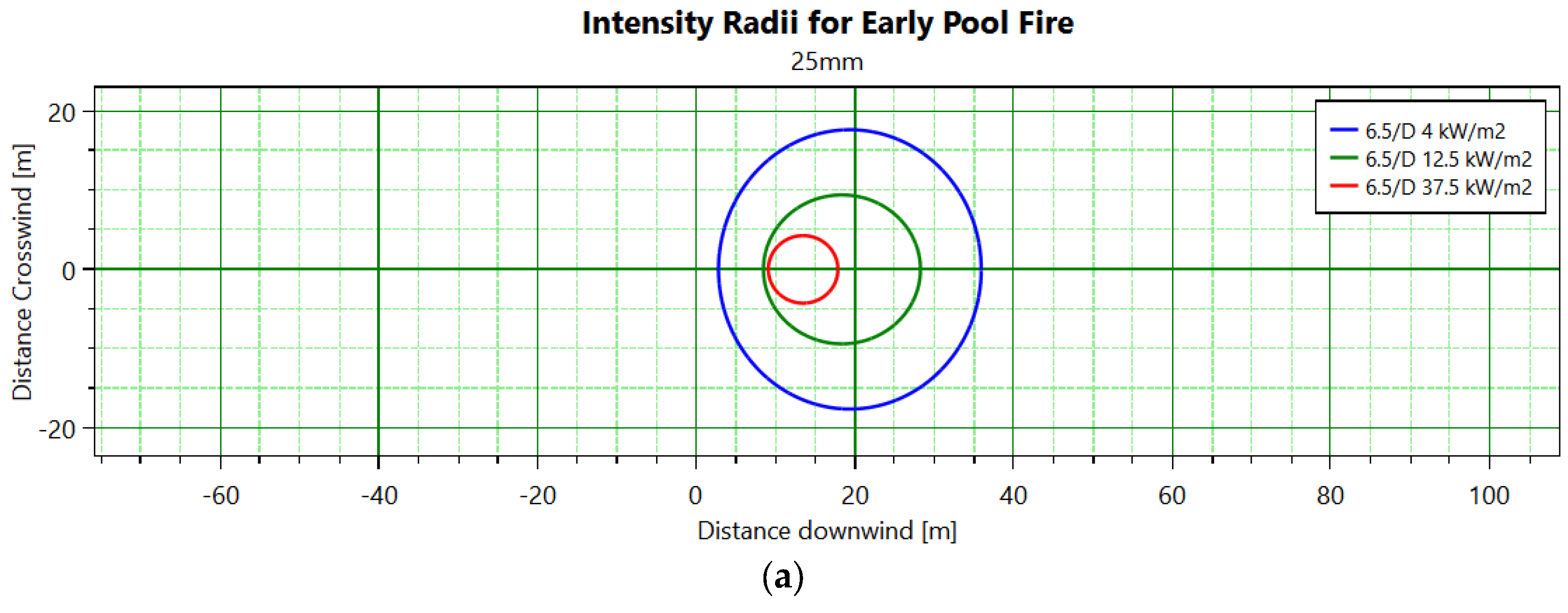
4.1. Case Study
4.2. Conclusions
Author Contributions
Funding
Data Availability Statement
Conflicts of Interest
References
- Lonzaga, J.B. Time reversal for localization of sources of infrasound signals in a windy stratified atmosphere. J. Acoust. Soc. Am. 2016, 139, 3053–3062. [Google Scholar] [CrossRef] [PubMed]
- Witlox, H.W.M.; Fernández, M.; Harper, M.; Oke, A.; Stene, J.; Xu, Y. Verification and validation of Phast consequence models for accidental releases of toxic or flammable chemicals to the atmosphere. J. Loss Prev. Process Ind. 2018, 55, 457–470. [Google Scholar] [CrossRef]
- Wu, T.; Wei, X.; Gao, X.; Han, J.; Huang, W. Study on the risk analysis and system safety integrity of enclosed ground flare. Therm. Sci. Eng. Prog. 2019, 10, 208–216. [Google Scholar] [CrossRef]
- Wang, K.; Zhou, M.; Zhang, S.; Ming, Y.; Shi, T.; Yang, F. Study on the Consequences of Accidents of High-Pressure Hydrogen Storage Vessel Groups in Hydrogen Refueling Stations. J. Saf. Environ. 2023, 23, 2024–2032. [Google Scholar] [CrossRef]
- Song, X.; Su, H.; Xie, Z. Numerical Simulation Study on Leakage and Explosion of LPG Tanker [J/OL]. Engineering Blasting:1-7. Available online: http://kns.cnki.net/kcms/detail/11.3675.TD.20231030.1022.002.html (accessed on 1 November 2023).
- Barros-Daza, M.J.; Luxbacher, K.D.; Lattimer, B.Y.; Hodges, J.L. Real time mine fire classification to support firefighter decision making. Fire Technol. 2022, 58, 1545–1578. [Google Scholar] [CrossRef]
- Ayhan, B.U.; Tokdemir, O.B. Accident analysis for construction safety using latent class clustering and artificial neural networks. J. Constr. Eng. Manag. 2020, 146, 04019114. [Google Scholar] [CrossRef]
- Hu, P.; Peng, X.; Tang, F. Prediction of maximum ceiling temperature of rectangular fire against wall in longitudinally ventilation tunnels: Experimental analysis and machine learning modeling. Tunn. Undergr. Space Technol. 2023, 140, 105275. [Google Scholar] [CrossRef]
- Khan, A.A.; Zhang, T.; Huang, X.; Usmani, A. Machine learning driven smart fire safety design of false ceiling and emergency response. Process Saf. Environ. Prot. 2023, 177, 1294–1306. [Google Scholar] [CrossRef]
- Rihan, M.; Bindajam, A.A.; Talukdar, S.; Shahfahad; Naikoo, M.W.; Mallick, J.; Rahman, A. Forest fire susceptibility mapping with sensitivity and uncertainty analysis using machine learning and deep learning algorithms. Adv. Space Res. 2023, 72, 426–443. [Google Scholar] [CrossRef]
- Sharma, R.; Rani, S.; Memon, I. A smart approach for fire prediction under uncertain conditions using machine learning. Multimed. Tools Appl. 2020, 79, 28155–28168. [Google Scholar] [CrossRef]
- Sun, Y.; Wang, J.; Zhu, W.; Yuan, S.; Hong, Y.; Mannan, M.S.; Wilhite, B. Development of consequent models for three categories of fire through artificial neural networks. Ind. Eng. Chem. Res. 2019, 59, 464–474. [Google Scholar] [CrossRef]
- Wang, R.; Chen, B.; Qiu, S.; Ma, L.; Zhu, Z.; Wang, Y.; Qiu, X. Hazardous source estimation using an artificial neural network, particle swarm optimization and a simulated annealing algorithm. Atmosphere 2018, 9, 119. [Google Scholar] [CrossRef]
- Yuan, S.; Jiao, Z.; Quddus, N.; Kwon, J.S.-I.; Mashuga, C.V. Developing quantitative structure–property relationship models to predict the upper flammability limit using machine learning. Ind. Eng. Chem. Res. 2019, 58, 3531–3537. [Google Scholar] [CrossRef]
- Sarbayev, M.; Yang, M.; Wang, H. Risk assessment of process systems by mapping fault tree into artificial neural network. J. Loss Prev. Process Ind. 2019, 60, 203–212. [Google Scholar] [CrossRef]
- Jiao, Z.; Ji, C.; Sun, Y.; Hong, Y.; Wang, Q. Deep learning based quantitative property-consequence relationship (QPCR) models for toxic dispersion prediction. Process Saf. Environ. Prot. 2021, 152, 352–360. [Google Scholar] [CrossRef]
- Sathesh, T.; Shih, Y.C. Optimized deep learning-based prediction model for chiller performance prediction. Data Knowl. Eng. 2023, 144, 102120. [Google Scholar] [CrossRef]
- Khodadadi-Mousiri, A.; Yaghoot-Nezhada, A.; Sadeghi-Yarandi, M.; Soltanzadeh, A. Consequence modeling and root cause analysis (RCA) of the real explosion of a methane pressure vessel in a gas refinery. Heliyon 2023, 9, e14628. [Google Scholar] [CrossRef] [PubMed]
- Mahesh, B. Machine learning algorithms-a review. Int. J. Sci. Res. (IJSR) 2020, 9, 381–386. [Google Scholar]
- Sun, B.; Liu, X.; Xu, Z.D.; Xu, D. BP neural network-based adaptive spatial-temporal data generation technology for predicting ceiling temperature in tunnel fire and full-scale experimental verification. Fire Saf. J. 2022, 130, 103577. [Google Scholar] [CrossRef]
- Smith, S.L.; Kindermans, P.J.; Ying, C.; Le, Q.V. Don’t decay the learning rate, increase the batch size. arXiv 2017, arXiv:1711.00489. [Google Scholar]
- Yan, S. Dynamic Adaptive Risk Assessment System for Individual Building Fires Based on Internet of Things and Deep Neural Networks. Master’s Thesis, China University of Mining and Technology, Xuzhou, China, 2021. [Google Scholar] [CrossRef]
- He, J.; Li, L.; Xu, J.; Zheng, C. ReLU deep neural networks and linear finite elements. arXiv 2018, arXiv:1807.03973. [Google Scholar]
- Friedman, J.H. Stochastic gradient boosting. Comput. Stat. Data Anal. 2002, 38, 367–378. [Google Scholar] [CrossRef]
- Biau, G.; Scornet, E. A random forest guided tour. Test 2016, 25, 197–227. [Google Scholar] [CrossRef]
- Rodriguez, J.D.; Perez, A.; Lozano, J.A. Sensitivity analysis of k-fold cross validation in prediction error estimation. IEEE Trans. Pattern Anal. Mach. Intell. 2009, 32, 569–575. [Google Scholar] [CrossRef] [PubMed]
- Cohen, I.; Huang, Y.; Chen, J.; Benesty, J. Pearson correlation coefficient. Noise Reduct. Speech Process. 2009, 2, 1–4. [Google Scholar] [CrossRef]
- O’brien, R.M. A caution regarding rules of thumb for variance inflation factors. Qual. Quant. 2007, 41, 673–690. [Google Scholar] [CrossRef]


| Area (m3) | Specification Model | Quantity | Capacity (m3) | Storage Medium |
|---|---|---|---|---|
| 1 | Φ60 × 19.92 | 4 | 50,000 | diesel fuel |
| 2 | Φ38 × 19.8 | 8 | 20,000 | gasoline |
| 3 | Φ22 × 14.852 | 1 | 5000 | diesel fuel |
| 3 | Φ22 × 14.852 | 1 | 5000 | gasoline |
| 4 | Φ8.920 × 12.565 | 2 | 500 | gasoline |
| 4 | Φ8.920 × 12.565 | 2 | 500 | diesel fuel |
| Range | Interval | Total Category | |
|---|---|---|---|
| Leakage pore size/(mm) | 5mm-Catastroptic rupture | 5/10/15 | 10 |
| stability | A-G | - | 10 |
| Wind velocity/(m/s) | 1-16 m/s | 1 | 16 |
| Material | N-OCTANE N-OCTADECANE N-HEXADECANE | - | 3 |
| Capacity/(m3) | 500, 500, 5000, 20000, 50000 | - | 5 |
| Leakage Pore Size/mm | Tank Materials | Volume/m3 | Filling Level | Temperature/°C | Wind Velocity/(m/s) |
|---|---|---|---|---|---|
| 5 mm | N-HEXADECANE | 50,000 | 80% | 25 | 1 |
| Incident Intensity/(kW/m2) | Damage to Equipment | Injury to Individuals |
|---|---|---|
| 37.5 | Complete damage to the operating equipment | 1% death (10 s) 100% death (1 min) |
| 25 | The minimum energy required for wood combustion under flameless, prolonged radiation | Severe burns (10 s) 100% death (1 min) |
| 12.5 | The minimum energy required for wood combustion and plastic melting in the presence of flames | First-degree burn (10 s) 1% death (1 min) |
| 4 | - | Pain lasting for more than 20 s, not necessarily accompanied by blisters |
| 1.6 | - | Long-term radiation without any discomfort |
| Number of Hidden Layers | Number of Neurons in Hidden Layer 1 | Number of Neurons in Hidden Layer 2 | Number of Iterations | Learning Rate | |
|---|---|---|---|---|---|
| 1 | 1 | 14 | - | 100 | 0.001 |
| 2 | 1 | 14 | - | 150 | 0.001 |
| 3 | 1 | 14 | - | 150 | 0.01 |
| 4 | 1 | 24 | - | 150 | 0.01 |
| 5 | 1 | 24 | - | 150 | 0.001 |
| 6 | 2 | 14 | 5 | 150 | 0.001 |
| 7 | 2 | 24 | 5 | 100 | 0.01 |
| 8 | 2 | 24 | 5 | 150 | 0.01 |
| 9 | 2 | 24 | 10 | 150 | 0.01 |
| NO | Variable | VIF | Tol |
|---|---|---|---|
| 1 | Leakage_pore_size | 1.00 | 0.97 |
| 2 | Capacity | 1.227 | 0.814 |
| 3 | Wind_Velocity | 1.00 | 0.97 |
| 4 | Temperature | 1.00 | 0.972 |
| 5 | Material | 1.227 | 0.814 |
| 6 | Stability | 2.0716 | 0.4827 |
| Jet Fire | Early Pool Fire | Late Pool Fire | ||||
|---|---|---|---|---|---|---|
| Evaluation | MSE | R2_score | MSE | R2_score | MSE | R2_score |
| BP | 0.008 | 0.945 | 0.004 | 0.986 | 0.017 | 0.968 |
| RandomForest | 0.010 | 0.945 | 0.010 | 0.954 | 0.084 | 0.888 |
| K-R | 0.0005 | 0.997 | 0.0004 | 0.997 | 0.0007 | 0.998 |
Disclaimer/Publisher’s Note: The statements, opinions and data contained in all publications are solely those of the individual author(s) and contributor(s) and not of MDPI and/or the editor(s). MDPI and/or the editor(s) disclaim responsibility for any injury to people or property resulting from any ideas, methods, instructions or products referred to in the content. |
© 2024 by the authors. Licensee MDPI, Basel, Switzerland. This article is an open access article distributed under the terms and conditions of the Creative Commons Attribution (CC BY) license (https://creativecommons.org/licenses/by/4.0/).
Share and Cite
Zhong, W.; Wang, S.; Wu, T.; Gao, X.; Liang, T. Optimized Machine Learning Model for Fire Consequence Prediction. Fire 2024, 7, 114. https://doi.org/10.3390/fire7040114
Zhong W, Wang S, Wu T, Gao X, Liang T. Optimized Machine Learning Model for Fire Consequence Prediction. Fire. 2024; 7(4):114. https://doi.org/10.3390/fire7040114
Chicago/Turabian StyleZhong, Wei, Shuangli Wang, Tan Wu, Xiaolei Gao, and Tianshui Liang. 2024. "Optimized Machine Learning Model for Fire Consequence Prediction" Fire 7, no. 4: 114. https://doi.org/10.3390/fire7040114
APA StyleZhong, W., Wang, S., Wu, T., Gao, X., & Liang, T. (2024). Optimized Machine Learning Model for Fire Consequence Prediction. Fire, 7(4), 114. https://doi.org/10.3390/fire7040114