It’s about Time: A Method for Estimating Wildfire Arrival and Weather Conditions at Field-Sampled Locations

Abstract

Weather conditions at the time of wildfire front arrival strongly influence fire behavior and effects, yet few methods exist for estimating weather conditions more spatio-temporally resolved than coarse-grain (e.g., 4 km) daily averages. When a fire front advances rapidly and weather conditions are heterogeneous over space and time, greater spatio-temporal precision is required to accurately link fire weather to observed fire effects. To identify the influence of fire weather on fire effects observed across a sample of existing forest inventory plots during a wind-driven megafire event in the US Pacific Northwest, we explored and compared three methods for estimating time of fire arrival and the wind speed at that arrival time for each plot location. Two methods were based on widely used, remotely sensed active fire data products with dissimilar spatial and temporal resolutions. The third and preferred method, Modeled-Weather Interpolated Perimeters (MoWIP), is a new approach that leveraged fine-grained (1.3 km, hourly) wind speed and direction from modeled fire weather to guide interpolation of aerial infrared-detected (IR) operational perimeters, subdividing the time intervals defined by sequential IR perimeters into quartile intervals to enhance temporal resolution of predicted fire arrival times. Our description of these fire arrival “time stamp” methods and discussion of their utility and shortcomings should prove useful to fire scientists, ecologists, land managers, and future analyses seeking to link estimated fire weather and observed fire effects.

1. Introduction

As megafires become the new normal and attract attention from researchers seeking to (i) understand how managing forest vegetation might reduce fire size and/or severity, or (ii) test and refine models that predict fire effects, linking meteorological data at a fine temporal scale to locations with pre- and post-fire measurements on the ground is both essential and challenging to accomplish with sufficient precision. Weather is widely understood to be the strongest driver of how fire burns when vegetation fuels are not critically limited, especially weather that is extreme (e.g., high winds and low humidity at the tails of their distributions [1]). Burgeoning information on vegetation status obtained from both remote sensing and from permanent plot monitoring systems, such as national forest inventories, offer opportunities to assess fire effects (e.g., vegetation mortality; combustion and charring of trees, plants, and soils) and the predictors of those effects. Although such data contain information on the structure and composition of vegetation fuels and their topographic context, predictors that may account for variation in fire severity and effects cannot be definitively identified and quantified without accounting for weather at the time a location burned, given the profound influence of wind and fuel moisture.

Retrospective analysis of fire effects does not comport with opportunities to establish weather sampling devices at locations of interest, whether those be locations of forest inventory plots or buildings and other infrastructure vulnerable to fire, even if the resources were available to support such instrumentation. Analysts must rely instead on existing networks of weather stations and models that downscale high-frequency weather observations from a limited number of distributed locations, such as stations in the Remote Automated Weather Stations (RAWS) network and atmospheric models applied to meteorological data contemporaneous with the fire. Such models and interpolations can also account for topography, to varying degrees, delivering an hourly to daily estimate for such fire-critical metrics as wind speed and direction, relative humidity, temperature, precipitation, and cumulative indices derived from temporal trajectories of these core metrics (e.g., fuel moisture deficits and drought indices).

When studying the intersection of fire and vegetation, the weather information that is often of greatest value is the subset that applies to when fire was actively burning at a particular location. Given that (i) weather is always changing, sometimes with dramatic transitions over time intervals on the order of an hour or two and (ii) the lack of precise information about where active fire is occurring (in real-time too, not just retrospectively), obtaining high accuracy, location-relevant fire weather remains an enormous challenge to those who pursue retrospective analyses. Availability of weather data covering every pixel of the landscape for every hour during a fire event is a necessary but not sufficient condition for incorporating weather into the analysis—the time of burning at particular locations is needed to exploit that data for the purposes just described.

Analysis of fire effects on vegetation is far from the only situation calling for precise characterization of where fire arrived, and when. For example, those who craft sophisticated models of wildfire smoke production and transport that couple numerical weather prediction models with atmospheric chemistry seek understanding of relationships among smoke production observed via terrestrial and airborne instrumentation that requires fire arrival times and the biomass available to the fire [2,3]. Such analysis is critical for building smoke prediction models that provide forecasts crucial for protecting human health from the effects of wildfire smoke. For these analysts, it is also a question of time, and considerable effort has recently been invested to improve interpolation techniques and implement machine learning to derive sub-daily arrival times for fire perimeters (e.g., [4,5]). Analysts exploring the influence of weather and vegetation fuels on fire behavior also need to know when fire arrives (e.g., [6,7]). Financial stakes in precise retrospective estimates of fire arrival time are rising fast—a jury awarded USD 73 million from the local power company to plaintiffs whose homes were burned at the time of Oregon’s 2020 Beachie Creek fire [8] on the grounds that the fires that burned their homes originated from arcing from electrical distribution system equipment that the company had neglected to deactivate, not from embers transported from the Beachie Creek fire—a conclusion reached based on modeling of fire arrival by expert witnesses [9].

For major fires over the past two decades in the U.S., National Infrared Operations (NIROPS) has produced fire progression perimeter polygons representing fire extents at variable intervals over the duration of a fire, derived via human interpretation of data from infrared (IR) sensors aboard aircraft. These perimeters, publicly available from the National Interagency Fire Center (NIFC) Operational Data Archive (https://data-nifc.opendata.arcgis.com/datasets, accessed on 10 May 2022), achieve relatively high spatial resolution (the underlying IR data are collected at 3 m scale) for the times of their collection. However, the timing of perimeter collection on active fires is irregular, corresponding to availability of aircraft and personnel resources and conditions that make safe overflights possible (e.g., a lack of high winds), and often occurs at time intervals (a day or longer)—too long to hope for fire arrival time precision for any particular location better than a day or two (except for locations that intersect an IR perimeter). Moreover, these data are typically collected only on major fire incidents, which, while covering most of the burned area, address a minority of the fire events. Notwithstanding these limitations, these perimeters are widely considered as close to “truth” as is available and are relied upon to constrain, train, or serve as reference data for fire progression perimeters derived from satellite-based active fire data products (e.g., [4,5]).

The approach to controlling for weather when analyzing fire effects in [10] is typical of how this information is used: (i) assign a burn “day” (somewhat complicated by IR perimeter intervals that can range from sub-day to multi-day and perimeters that rarely occur only at midnight) to each field plot based on overlay of the progression perimeters generated by NIROPS; (ii) extract from a weather station in the general vicinity, a vector of daily weather attributes (typically using observations collected at 1400 h local time, when weather is considered most likely to represent conditions most conducive to fire propagation, or an average of the hourly data from RAWS), and assign those attributes to all plots within the perimeter interval. Although fire arrival weather computed this way may be representative and valid in some cases (e.g., if weather attributes remain largely unchanged over the IR perimeter interval), any variation in weather over that interval introduces imprecision that can compromise detection of significant non-weather predictors of fire effects (e.g., vegetation).

Until very recently, the literature has provided essentially no guidance on determining when the expanding perimeter of a fire arrived at any arbitrary location—i.e., the time at which combustion of fuels began at that location. This is precisely the information required for retrospective analysis of fire effects, forensic attribution of fire damages to ignition sources, and definitive modeling of wildfire smoke production and propagation. Available data that could help precisely identify a burn time tends to be opportunistic, highly variable, and poorly documented. During a fire suppression incident, the incident commander’s responsibility for the safety of firefighters requires maintaining a situational awareness that demands attention to where fire is burning and prediction of where it will burn next. The voluminous collection of structured and unstructured data and generation of operations maps during a fire incident supports this need, not the interests of future analysts to conduct retrospective analysis on fire effects. It is thus less than surprising that much of this data are ad hoc, lightly documented at best, and only partially preserved and that the IR perimeters produced by NIROPS mainly on large fires are the only consistently available event-focused information that can address the timing of fire arrival.

The need for retrospective fire growth data is beginning to be recognized and addressed by analyses that rely on active fire sensors aboard satellite platforms such as Geostationary Operational Environmental Satellite (GOES), Moderate Resolution Imaging Spectroradiometer (MODIS), and Visible Infrared Imaging Radiometer Suite (VIIRS), sometimes augmented with IR perimeters from NIROPS (e.g., [4,5,11]). A laudable motivation for these efforts is building a nationally consistent, automated system for generating reliable fire arrival information that yields cumulative burned area over time for all incidents, not just those covered by NIROPS, along with fire arrival times. Most of these studies attempt some kind of validation via scoring systems, such as those based on fire arrival time agreement and shape agreement developed by [12] to evaluate fire propagation simulations. These efforts do not appear to have achieved sub-daily temporal precision on fire arrival estimates required for the kinds of application described earlier. This is likely due to potentially intractable limitations of the active fire data, including temporal infrequency (twice daily for MODIS and VIIRS) and lack of synchronization with NIROPS IR perimeter collection times that would enable more definitive validation but more fundamentally by large pixels/distance separating detections (especially with the high temporal frequency GOES data and its multi-kilometer pixel size, but also for the others). An indeterminate proportion of pixel area must have sufficient combustion occurring to elevate the IR signal above a “background” value for that pixel to be classified as actively burning, and that calculus becomes even more problematic across heterogeneous topography and land cover. Moreover, whatever threshold is selected, there will likely be unburned area within the pixel for which fire arrival will certainly be later than the satellite-based active fire sensor derived representation of fire arrival.

Obtaining the most representative time to link weather data to a location that burns (so as to account for weather when evaluating the influence of non-weather predictors of observed fire effects) is further complicated by the considerable variability in fire residence time, which may be conceived as dependent on weather and fuels, and ranging from less than an hour to days, or longer (e.g., when below-ground combustion continues long after the flames have subsided, sometimes for months). Still, fire behavior at the time of arrival—particularly the intensity produced when flames are most active—is relevant for explaining many fire effect responses such as tree mortality, tree bole and crown scorch, and combustion and charring of soils. Successfully linking location appropriate weather to fire arrival time (what we define as a “time stamp”) at a location has the potential to explain many of the most important fire effects. Even with imprecision in fire arrival time and therefore weather metrics linked to that time, it is helpful to identify a weather class, for example, a wind speed range, so that analyses of drivers like vegetation structure can consider and control for weather when exploring relationships between fire effects and factors over which management practices may exert some control.

This paper presents and evaluates a protocol we developed to assign a temporally resolved time stamp of fire front arrival to Forest Inventory and Analysis (FIA) plots nested within a forested landscape extensively burned by a wind-driven megafire event, referred to hereafter as the 2020 Labor Day Fires, in the US Pacific Northwest. This protocol was developed specifically to link observed fire effects on FIA plots to fire weather in a separate but related study [13]. We pursued three alternative approaches to identifying fire arrival time at each FIA plot. Each alternative follows a different conceptual framework and spatial representation: (i) VIIRS—remotely sensed “hot spot” points that appear and then disappear (when cooled) but are only sampled at ~12 h intervals; (ii) GOES—coarse (2 × 4 km) grid cells that take on a “fire present” status when an indeterminate proportion of the cell is on fire, populated on a 5–15 min interval; and (iii) NIROPS-provided IR perimeters—as a spreading front represented by perimeters collected at irregular intervals (from hours to days, though usually at least once daily when fire behavior is most active), primarily via interpretation of infrared overflights. Relying on IR perimeters as a close to “ground truth” approximation of arrival time at the location of plots in the vicinity of these perimeters, we evaluated differences among methods in (i) predicted fire arrival time and (ii) predicted wind speed derived from those predicted arrival times at each FIA plot.

2. Materials and Methods

All data processing and analyses were performed using R Statistical Software ver. 4.2.2 [14] and ESRI ArcDesktop ver 10.8 [15]. Throughout this manuscript, R packages are identified by quotation marks and cited. The ESRI GIS tools are written in uppercase followed by the associated ArcMap toolboxes in brackets.

2.1. Data

2.1.1. Fire Progression—GIS Perimeter Layers Derived via Infrared Overflights

We accessed the NIROPS IR-perimeters for six contemporaneous fire events in the western Oregon and Washington Cascades that comprise the 2020 Labor Day Fires from the National Interagency Fire Center (NIFC) Operational Data Archive geodatabases (https://data-nifc.opendata.arcgis.com/datasets, accessed on 5 May 2022). Consistent with reports by other researchers attempting to make use of NIROPS IR perimeters for post-fire analysis (e.g., [4,5]), these data exhibit multiple anomalies, including redundancies and inconsistencies that might be expected for data intended to support tactical scale management of an ongoing wildfire, where timely delivery takes precedence over data cleanliness. For example, there are 152 polygons of IR data for the Beachie Creek Fire, each with multiple “time stamp” variables recorded (i.e., CreateDate, DateCurrent, and PolygonDateTime) expressed in coordinated universal time (UTC). These variables often prove to be inconsistent and require additional data exploration to identify a time of collection in which one can have confidence. After reviewing the metadata, we found the PolygonDateTime to be the most reliable, but for several perimeters, this field was unpopulated. We chose not to rely solely upon CreateDate or DateCurrent in lieu of the null PolygonDateTime values and instead used those fields in conjunction with fire data logs; reported changes in fire area growth; alignment with IR points, lines, and polygons detected via overflights; and congruence with KMZ (Google Earth) files downloaded from the NIFC Incident Specific Data website (https://ftp.wildfire.gov/public/incident_specific_data, accessed on 15 June 2022). We applied a cleaning and reconciliation process to arrive at a final set of what we refer to in this paper as “IR perimeters,” suitable for the interpolation analysis that is the core of the approach we tested and recommend. Our selection process began by removing (i) all redundant (or very similar) perimeters, (ii) perimeters with missing time stamps that could not be reconciled with other information sources, and (iii) perimeters that fell well outside our time of focus for each fire incident that comprised the 2020 Labor Day Fires (generally 7–15 September 2020).

For the purpose of comparing fire arrival time stamp assignment approaches in this study, we assumed that the remediated IR perimeters represent true fire progression. Given the absence of more precise data sources, we relied on this “ground truth” as the basis for comparing predictions of all three methods.

2.1.2. Fire Detection—Satellite-Based Point and Raster Remote Sensing Datasets

Two remotely sensed, satellite-based active fire detection products were also used to estimate time of fire arrival:

• The VIIRS instrument exhibits a high spatial resolution of ~375 m but relatively coarse temporal resolution consisting of single day and night overpasses approximately every twelve hours (https://www.earthdata.nasa.gov/learn/find-data/near-real-time/viirs, accessed on 30 May 2022). We processed raw VIIRS data, a shapefile of fire detection points that includes a time stamp attribute, into a gridded 500 m resolution raster surface representing the first day and time that fire was detected within each pixel. Setting the raster resolution to 500 m ensured at least one VIIRS fire detection point fell within each pixel boundary across the raster surface, preventing cells from taking on null values. If more than one fire detection point fell within a pixel boundary, we used the earliest time stamp value among the points to represent the pixel value (i.e., via the minimum function).
• The Advanced Baseline Imager (ABI) onboard the two Geostationary Operational Environmental Satellite-R (GOES-R) uses active fire data from the 30 m multi-spectral Landsat 8 to produce imagery covering a 5000 km (east/west) by 3000 km (north/south) rectangle over North and South America (https://www.goes-r.gov/products/overview.html, accessed on 25 June 2022). The GOES datasets are in the NetCDF format commonly used for climate data and other large multidimensional arrays and gridded datasets. This format provides climate attribute values and associated metadata such as latitude, longitude, and attribute labels and is transferable across different operating systems and software platforms. Preprocessing in R was completed using the package “ncdf4” [16]. The spatial and temporal resolution of data from GOES ranges from 0.5 to 4 km and from 5 to 15 min, respectively. The satellites are positioned over the equator at 75.2° W (GOES-16) and 137.2° W (GOES-17). Although our analysis centered on the 2020 megafires in western Oregon and southwest Washington (closer to GOES-17) we relied on GOES-16, which is optimized for the eastern US, thereby accepting decreased spatial resolution near the edge of the field of view (~4 km) owing to concerns over the technical accuracy of GOES-17 [17].

2.1.3. Weather

Given the high variability in weather conditions observed across the fire event during the majority of fire growth period (7–9 September) and the extent of FIA plots (~1 ha), it was important to account for weather conditions using weather data with high spatial and temporal resolutions. This led us to rely on output from a Weather Research and Forecasting (WRF) model, as described by [18], to estimate hourly weather data at a 1.3 km gridded spatial resolution. These data were used to characterize wind speed and other important fire weather attributes (wind direction, temperature, and relative humidity). Wind speed and direction were characterized at 10 m, and temperature and relative humidity, 2 m, above ground level.

2.2. Interpolated Infrared Fire Perimeters Approach

Our interpolation approach, which we refer to as the Modeled-Weather Interpolated Perimeters (MoWIP), starts with NIROPS IR perimeters, initially mapped to support fire operations and subsequently refined to assure quality, and interpolates fire growth over time based on modeled, gridded, hourly weather data from the WRF model. To assign a time stamp to each plot, we processed each individual fire incident (out of six total) as follows:

• Starting from the innermost IR perimeter or fire origin “point” (which is often represented as a very small perimeter in the NIROPS data), we selected each IR perimeter (after cleaning and removal of redundant representations) and the next larger IR perimeter in which it is nested, noting their time stamps to calculate a time interval, t, separating these two perimeters. We then divided t into four analysis periods, each of length t/4. We determined that subdividing perimeter intervals into more than four analysis periods might yield more accurate time stamps and sometimes also weather estimates, depending on length of the perimeter collection interval and degree of weather variability, but at greater analytic cost and with diminishing returns. Over the first five days following the ignitions of these fires (~6–10 September), intervals separating IR perimeters ranged from approximately 2 to 63 h; thus, the duration of the analysis periods for which interpolated perimeters needed to be delineated to translate those time increments into fire growth ranged from less than 1 to ~16 h.
• To inform the placement of each interpolated perimeter, we developed gridded raster surfaces containing the mean wind speed from the WRF model over each multi-hour analysis period within the interval between IR perimeters. Mean wind speed was calculated for each analysis period from the hourly WRF wind speed in that period using the RASTER CALCULATOR [Spatial Analyst Tools/Map Algebra] tool. If the total time interval between IR perimeters was not evenly divisible by 4, we assigned the modulus to the last period (e.g., if 15 h, then periods 1–3 were 4 h each and period 4 was 3 h).
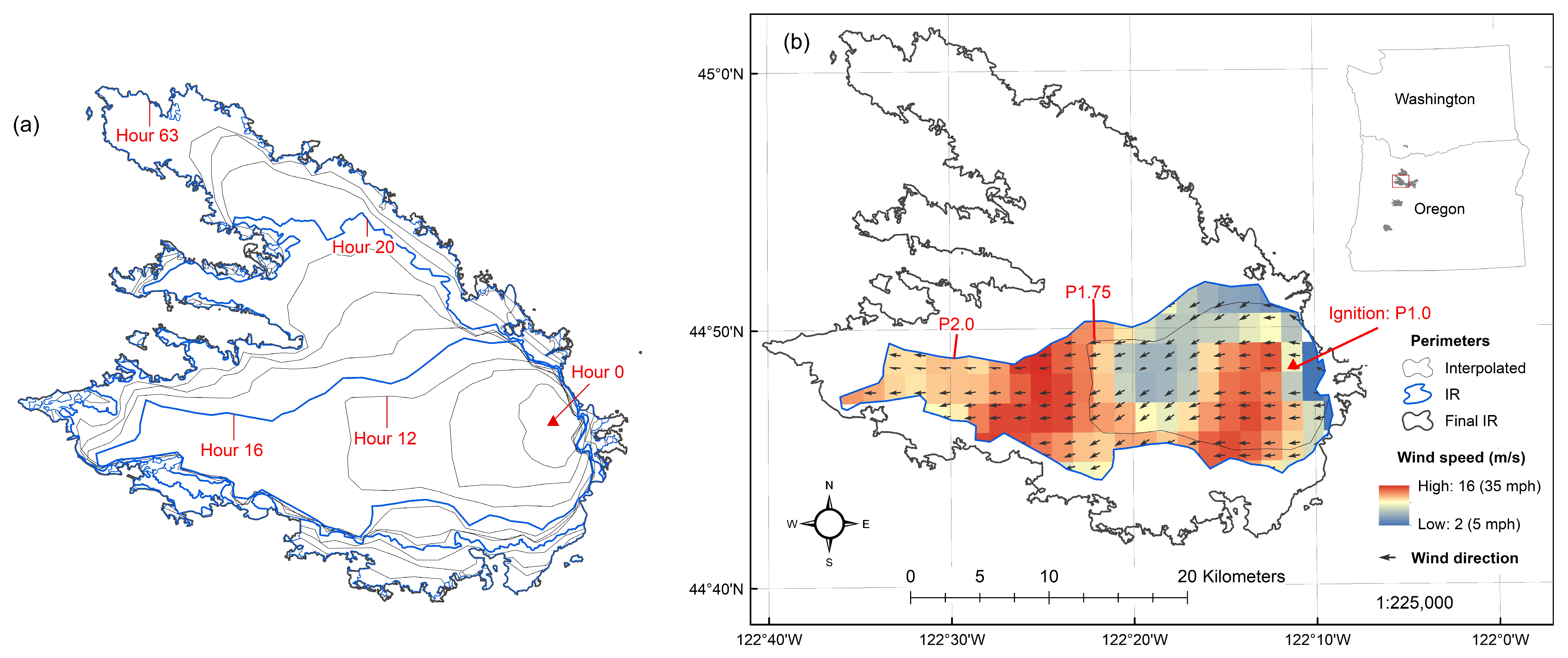
• Wind direction rasters were (i) symbolized as vector fields (wind arrows) for visualization at ~2.5 km scale (Figure 1), and (ii) converted to vector points to calculate a one standard deviation ellipse covering 68% of these vectors for each analysis period with the DIRECTIONAL DISTRIBUTION [Spatial Statistics/Measuring Geographic Distributions] tool. The orientation of the ellipse (not displayed in Figure 1) depicts mean wind direction for that period, providing a helpful visual reference that informed the drafting of interpolated perimeters. All three guidance layers could be toggled on and off, iterating forward and backward in time, during interpolation (Figure 1).
• Fire spread regularity guides the mechanics of interpolation:
  • When fire spread was relatively homogeneous over the length of the previous IR perimeter such that the shape was relatively regular (most common when wind was low and spread was slow), we crafted preliminary interpolated perimeters by resizing copies of a IR perimeter, stretching, and warping as needed to reflect wind speed and direction.
  • When fire spread demonstrated asymmetry or irregularity, such that the perimeter shape was directionally heterogeneous (most common when wind was high and spread was rapid or varied among regions of the perimeter), we manually sketched interpolated perimeters, guided by the same information.
• Interpolated perimeter graphic objects were converted to polygon shapefiles. When nested IR perimeter pairs were separated by short time or short distance, we did not attempt to interpolate between them, in part because in many cases there was literally no space in which to insert a perimeter (nested perimeters with different time stamps were spatially coincident, at least for some perimeter segments) or there was “negative space” (when a later time stamped perimeter was paradoxically inside of an earlier time stamped perimeter, typically owing to errors in the IR perimeters that present no obvious resolutions).
• This process was repeated for each nested IR perimeter pair for which partitioning was viable, resulting in 1–3 groups of interpolated perimeters per fire incident. This provided an additional 3–9 interpolated perimeters for each fire incident, enabling more temporally resolved weather assignment to each plot during the time when fire spread was most active (Figure 1).

All perimeters, IR and interpolated, were integrated into a master shapefile and assigned perimeter sequence numbers, most easily described via the example for the Beachie Creek fire shown in Figure 1: the first IR perimeter, P1.0, is the ignition; the second IR perimeter is P2.0; and the interpolated perimeters that divide the time interval between P1.0 and P2.0 into four nearly equal periods are P1.25, P1.50 and P1.75. To each analysis period (named for the outer bounding perimeter), we assigned a timestamp midway between the timestamps of the outer and inner perimeters for that period so that an approximate fire arrival time stamp for each plot could be assigned via overlay.

The overlay was accomplished via geometric intersection of all perimeters in the master shapefile and all plot locations via the INTERSECT [Proximity] tool, which appended the plot relevant time stamp associated with the intersected perimeters to the output feature class. We filtered the data table to the earliest timestamp associated with each plot and used those time stamps to extract weather attributes for that plot from the WRF raster cell coincident with that plot.

2.3. Data Quality Challenges for Implementing MoWIP

2.3.1. Date Systems

Integration and alignment of quite a few data sets, each with their own format (tabular, raster, vector, and imagery) and from sources not entirely consistent in how they report data collection time presented significant obstacles. Most remotely sensed products are recorded in universal time (UT), a 24 h format that is the world’s standard time keeping scale to facilitate synchronization (i.e., coordination) across agencies, therefore “Coordinated Universal Time” or UTC with the Prime Meridian (0° longitude) that passes through the Royal Observatory in Greenwich, London as the reference starting point. In the metadata, UTC is sometimes referenced as International Time, Zulu Time (U.S. military), or Greenwich Mean Time (GMT).

When data are reported in different systems accounting for time, they must be reconciled to a common system before analysis. For example, we relied on multiple remotely sensed data for which time was recorded in UTC and IR data collected from aircraft that, in some cases, recorded time in Pacific Standard Time (PST), even though Pacific daylight savings time (PDT) was used for local time when the fires occurred. We converted all time variables (e.g., from remote sensing, weather models, and fire perimeters) into our own system: decimal hours since midnight local (PDT) time 1 September 2020 (with the midnight separating September from August as hour zero).

2.3.2. Positional Inconsistencies in Fire Perimeters over Time

It appears that each fire progression polygon is developed, either by observers during fire overflights or interpretation of infrared imagery following an overflight, independently from and without efforts to reconcile against previously generated progression polygons. We reached this surmise thanks to anomalies like the one depicted in Figure 2, in which polygons representing the fire’s progress at different points in time intersect. It is understandable that such reconciliation may not be required for progression perimeters to be useful during fire management operations; however, this lack of reconciliation presents problems when relying on progression perimeters as a reference for fire arrival to points on the ground. Perimeters that regress rather than progress (over some portion) can, in some cases, be a valid representation of what occurred (e.g., when a fire reburns and reactivates portions of a spot fire already mapped). At other times, regression may result from inaccurate mapping, for example, when an area thought to have burned on Day 1 is determined on Day 2 not to have burned, yielding negative expansion (i.e., contraction) of a portion of Day 2’s fire progression perimeter, relative to Day 1. These anomalies are especially common when perimeters are developed for days on which fire spreads very slowly, if at all, and may result from digitizing error, given that the purpose of their delineation was to manage fire operations and safety, not to generate accurate fire arrival times for retrospective analysis. Whatever their cause, such anomalies complicate the interpolation task in the MoWIP approach, requiring close inspection and correction (via editing of polygon vertices) prior to geoprocessing.

2.4. Time Stamp Adjustment and Assignment from Remotely Sensed Detection of Thermal Anomalies

Given the coarse spatial resolution (~4 km) of the GOES active fire data, this product may be systematically biased toward early fire detection. Only a portion of the 4 km GOES cell needs to be actively burning to flag the entire cell as burning; if the fire front intersects the east (upwind) edge of a pixel but the plot of interest is near the west edge of the pixel, the actual time of fire arrival to the plot may be much later than indicated by the time coded for the pixel. To reduce the magnitude of such discrepancies, we (i) interpolated GOES time values to a higher spatial resolution using the EMPIRICAL BAYESIAN KRIGING [Geostatistical Analyst] tool, (ii) converted the resulting geostatistical layer to a raster grid, and (iii) geographically shifted it 2 km eastward (accounting for the movement of the leading edge of the fires from east to west) to partially offset the early fire detection effect embedded in the GOES data.

A SPATIAL JOIN [Analysis Tools with Match Option = Closest] of FIA plot locations and the raster time stamp (in hours since September 1st) generated from the VIIRS- and GOES-based methods was used to assign a fire detection time stamp to each plot.

2.5. Comparison of Method Outcomes for Reference Plots near IR Perimeters

To assess potential discrepancies among the three fire arrival time methods explored in this study, we compared the MoWIP time stamping and weather assignment methods, relative to the two remotely sensed, satellite-based active fire product approaches for plots that were near an IR fire progression perimeter (not the interpolated ones). We assumed that the IR perimeters, as problematic as their precision may be, are likely the closest approximation to truth that is available—after all, the collection of these perimeters is motivated by the need to map the fire front at specific times to support and ensure safety for fire management operations. During the first three days of the 2020 Labor Day Fire complex, when the rapid rate of spread enabled by high winds led to very large distances between consecutive perimeters, we would expect that those perimeter time stamps would be close in time to the fire arrival at those nearby plots, to an extent that might not persist as declining wind speeds slow fire spread. We expected MoWIP time assignments to be close to, but not the same as, IR perimeter time stamps because those assigned times are mid-way between the perimeter time stamp of that close-by IR perimeter and the time stamp of the interpolated perimeter bounding the other end of the interval in which the plot sits.

We used the NEAR [Analysis Tools/Proximity] tool to calculate the planar distance between plots and IR perimeters (to identify the nearest one) after converting perimeter polygons to lines. We included only plots that fell within 200 m of an IR perimeter that was time stamped no later than the end of the third day of the fire, when winds had largely subsided. We designated the plots that met the timing and distance criteria as a reference dataset (n = 19). We calculated differences between the reference data time stamp (derived from the nearby IR perimeter) and the estimated plot time stamp for each time stamp estimation method (estimation method time stamp minus the nearest IR perimeter time stamp). We also calculated differences in wind speeds implied by these time stamps (between reference data and values estimated by each method) and explored patterns in these differences.

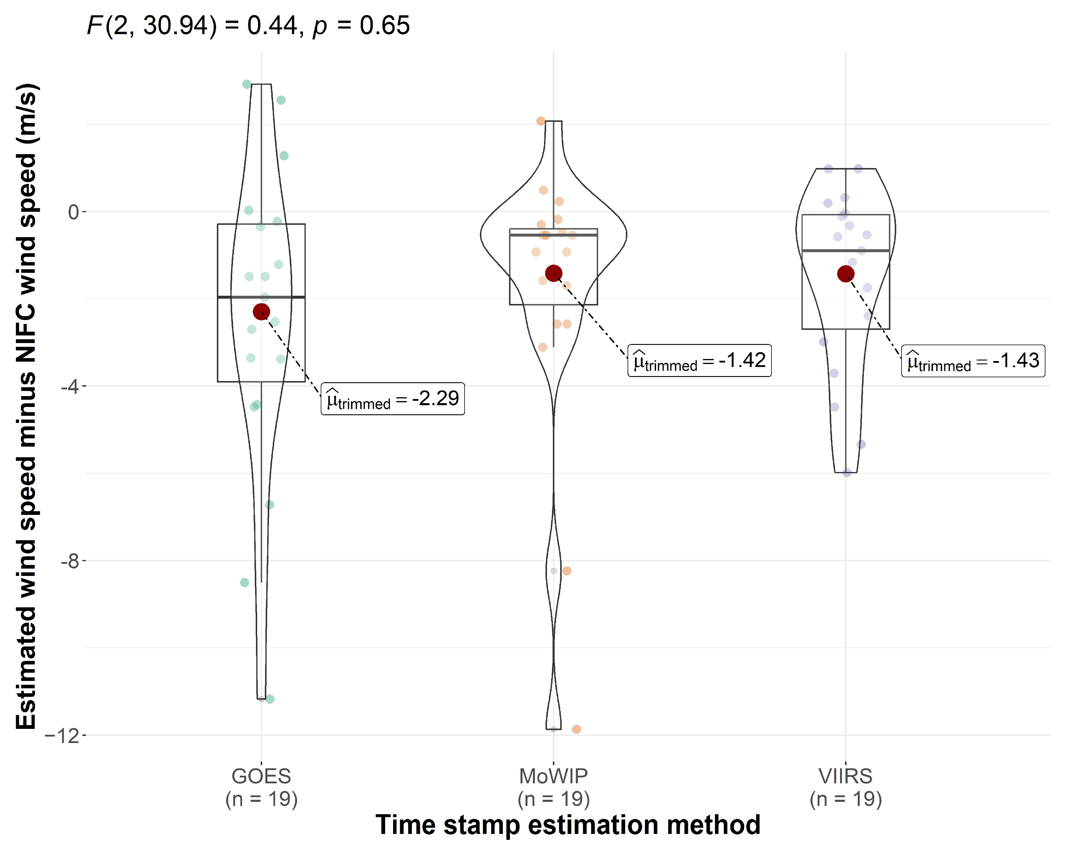
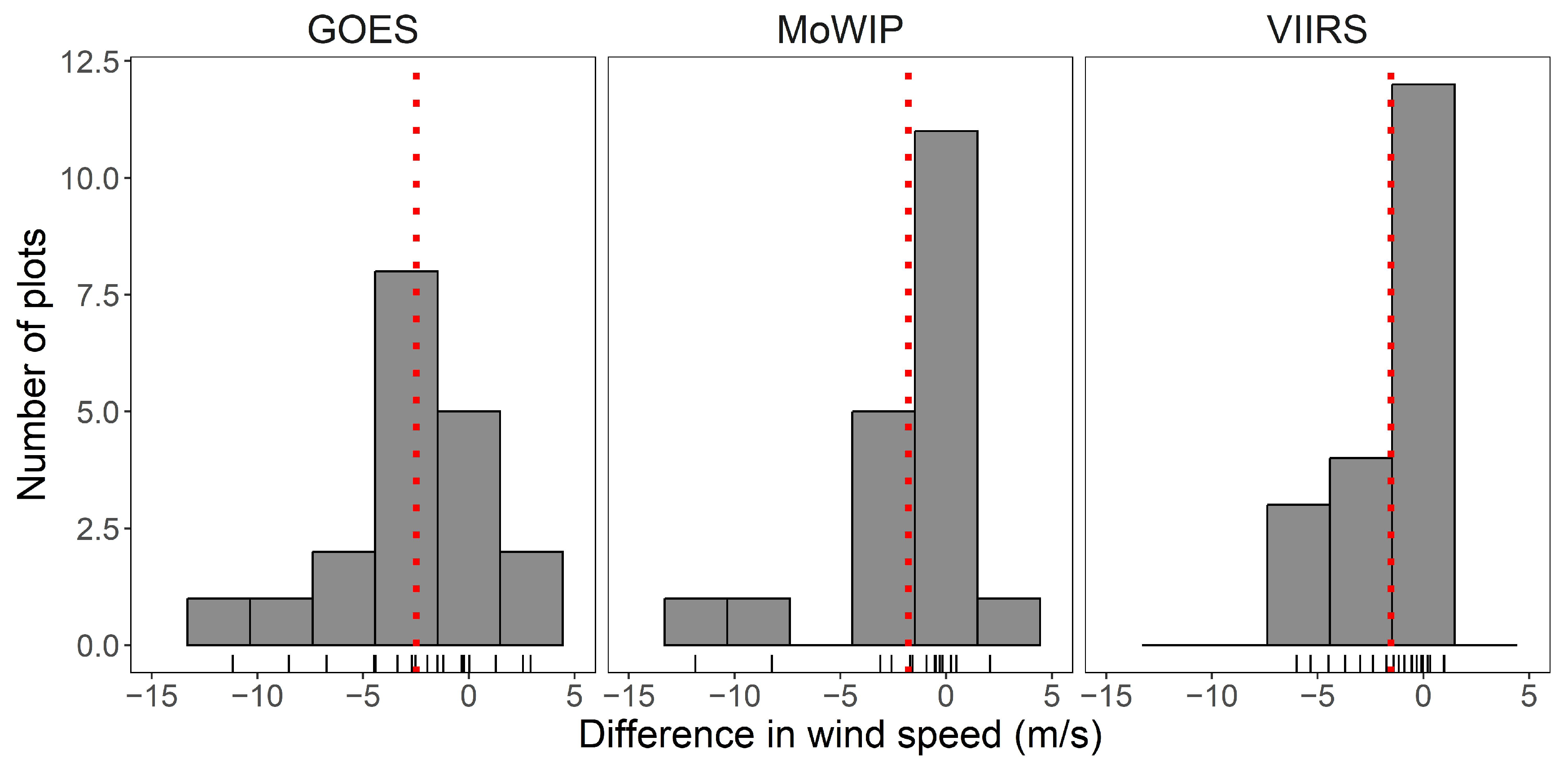
We tested the trimmed-means of the differences in time stamp and wind speed for each method as a robust estimate of central tendency with the R package “ggstatplot” [19]. The trimmed-mean provides a better estimate of where the bulk of the observations are found when sampling asymmetric distributions, as these proved to be. We set the trim function to 0.1 to remove 5% of the smallest and 5% of the highest values and then averaged the remaining observations. The median with non-parametric approaches is an example of an extreme trimmed mean. The standard error of the trimmed-mean is less influenced by outliers and asymmetry so this method has more power than tests using a simple mean. With the trimmed-means we visualized the distribution of the differences of the fire arrival time stamps and wind speeds as box plots with kernel density curves with default settings with the “tidyverse” R package suite [20]. Kernel density curves are a non-parametric method of estimating the probability density function of a continuous variable. The plots display a smoothed version of a histogram that provides better representation of distribution shape because kernel density curves are not subject to influence by the number of bins used in a histogram.

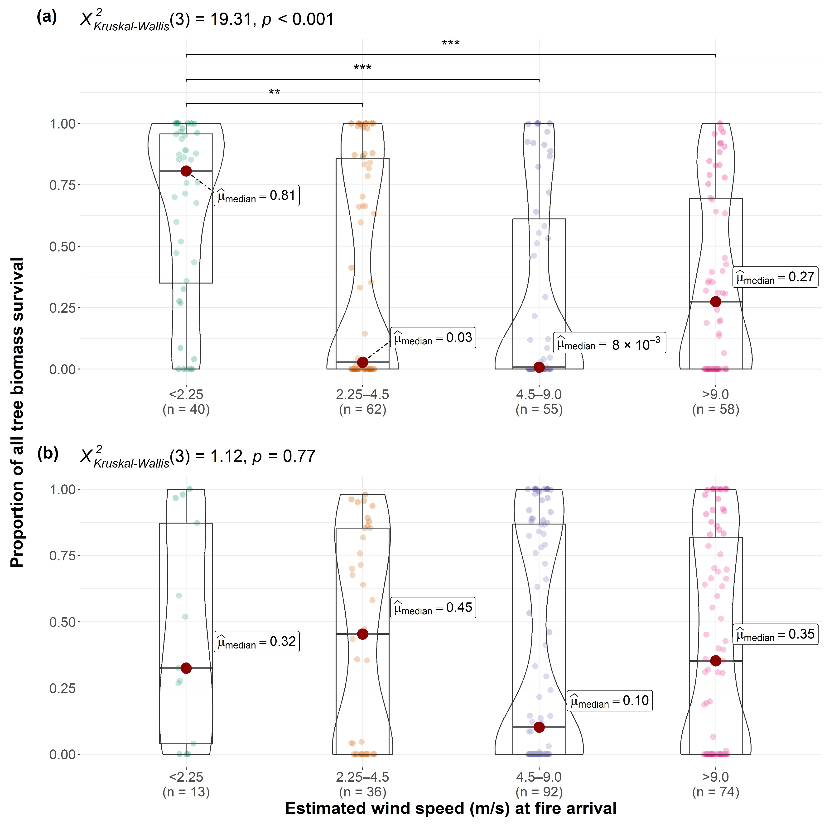
Finally, to illustrate the improved accuracy of wind speed at the estimated time of fire arrival derived via sub-daily MoWIP vs. more widely used daily estimation methods, we compared the distribution of proportional tree biomass survival responses observed across forested FIA conditions (full or partial FIA plots; n = 215) burned by the 2020 Labor Day Fires, one-year post-fire, using thresholds of estimated mean wind speed (<2.25, 2.25–4.5, 4.5–9.0, and >9.0 m/s). The derivation of the post-fire tree survival response data is described in detail by [2]. For the daily wind speed estimation method, we used the VIIRS active fire product (described above) to assign the first day an FIA plot was detected as within the fire. Mean daily wind speed was then extracted from the GRIDMET meteorological dataset [21] as a gridded 4 km raster surface to each plot location via spatial overlay. Informed by a large body of fire effects research, we expected that tree survival responses would be monotonic in nature and decrease with increasing mean wind speed. We hypothesized that poor estimation and assignment of mean wind speed at the time of fire arrival would result in a non-monotonic relationship between wind speed thresholds and tree survival and no statistical differences in tree survival across wind speed thresholds. We tested for statistical differences in tree survival responses across wind speed thresholds using a Kruskal–Wallis rank-sum test with a post hoc Dunn’s test with Holm correction for multiple pairwise comparisons.

3. Results

3.1. Time Stamps

The time stamps assigned were significantly different (p < 0.05) among methods for 19 reference plots located within 200 m of IR perimeters. The difference between trimmed means was closest to zero for MoWIP (Figure 3 and Figure 4). Consistent with our expectations, it is no surprise that two-thirds of the MoWIP assigned time stamps were within four hours of the IR perimeter time stamp and that the mean difference was less than a half-hour ($\overline{x}$ = 0.47, $s^2$ = 15.04), given the construction of this reference sample to include only plots within 200 m of an IR perimeter and the MOWIP time stamp depending so directly on IR perimeters. For MoWIP, the differences are primarily determined using the length of the analysis period with which a plot is associated and the fire spread rate during that period. The discrepancies for GOES ($\overline{x}$ = −7.53, $s^2$ = 159.49) and VIIRS-assigned time stamps ($\overline{x}$ = 31.37, $s^2$ = 103.91) are much greater, and with opposite signs. The GOES-assigned times for this reference sample were, on average, almost 10 h premature ($\overline{x}$_{Trimmed mean} = −8.5), likely owing to the first detection of fire at some location within a very large (4 km edge) pixel that may be quite distant from the plot. This was despite the “centering” adjustments we made to the GOES data, in an attempt to mitigate this expected issue. The few GOES-assigned times that were very late (by as much as 30 h) could have been caused by plots at the leading edge of a pixel where an approaching fire crept slowly onto the pixel, but only affected a sufficient proportion of it to generate an active fire signal much later. VIIRS-assigned times are in all cases tardy relative to the closest IR perimeter, with a mean lag of over 30 h. These very large time differentials may make it unlikely that weather assigned based on GOES and VIIRS will reflect conditions when a plot burned, unless weather remains homogeneous over time.

3.2. Wind Speed

We examined the extent to which differences in time stamp assignment between methods (estimated minus IR) affected wind speed assignment for the 19 reference plots located within 200 m of IR perimeters. The trimmed-means of the difference between wind speed calculated for a method’s time stamp assignment and that calculated for the time stamp of the nearest IR perimeter were similar across methods (Figure 5 and Figure 6), with a rank-based nonparametric comparison of median differences (χ²(2) = 1.27, p = 0.53), indicating no statistically significant differences among wind speed prediction methods for this small reference sample. However, the wind speed differences for MoWIP are more tightly clustered around zero and with a more pronounced modal peak ($\overline{x}$ = −1.78, $s^2$ = 10.25); the two outliers, at points interior to the IR perimeter, have a substantial influence on mean wind speed difference. A negative difference value and associated “in” status (meaning that they burned before the fire reached the IR perimeter; see caption for Figure 3) suggest that wind speed increased between the MoWIP-assigned time stamp (which is midway between the time of the IR perimeter and the next smallest interpolated perimeter) and the IR perimeter that the fire expanded to during this AP. Given a recent analysis indicating that wind speeds exceeding 2.25 m/s can drive high tree mortality [2], discrepancies on the order of even a couple of meters per second can make the difference between capturing fire relevant weather attributes or failing to do so.

3.3. Tree Survival

To illustrate potential improvement toward explaining fire effect responses when using sub-daily vs. daily estimation methods, we evaluated the relationship between field-observed tree survival responses across a large sample of forested FIA conditions (n = 215) burned by the 2020 Labor Day Fires, and mean wind speed at fire arrival estimates as derived via MoWIP and an alternative daily estimation method (Figure 7). Under the MoWIP method that utilizes sub-daily fire arrival times via interpolated IR perimeters and high-resolution hourly modeled weather data (a), mean and median tree survival decreases abruptly as wind speed increases. Statistical differences were detected between mild (<2.25 m/s) and moderate to strong (2.25–4.5, 4.5–9.0, and >9.0 m/s) wind speed thresholds as hypothesized, and following conventional understanding of fire weather and fire effects. Alternatively, under the daily estimation method (b), no discernable relationship exists between tree survival and thresholds of estimated wind speed at fire arrival, nor any statistical differences, indicating that wind speed estimates are not sufficiently accurate to account for the influence of weather on an important, observed fire effect (tree mortality).

4. Discussion

To understand how pre-fire stand structure and composition influence fire outcomes for soils and vegetation observed in the field post-fire, it is essential to account for site-level weather conditions. For questions relating to fire intensity and duration, weather, particularly wind, is often a driver at least as important as site conditions such as the fire resistance properties of the species that grow there, ground and canopy fuel structures, and loadings that reflect fire legacies and prior mitigation activities, if any [22].

The shapes of fire scars on the landscape reveal the complex interactions among wind speed and direction, fuels, and topography that influence fire progression. Many small fires burning under moderate weather conditions are round [23], constrained primarily by levels and homogeneity of vegetation fuels [24]. In contrast, most large wind-driven fires are elliptical as the head fire front spreads much faster than the flanking and backing fire fronts, and unpredictable changes in wind direction and speed over varying terrain produce irregular patterns of spread [25]. The 2020 Labor Day Fires spread rapidly from east to west under strong, east winds that only gradually subsided over the first three days of the fire [18], producing large, roughly elliptical fire scars and comparatively few, officially mapped perimeters over the three-day period during which winds gradually moderated from exceptionally extreme to calm. When the winds had fully subsided, fire spread slowed, resulting in intervals between successive IR perimeters that were long in time and short in distance. While this decreased the precision in time stamp assignment and confidence that the weather assigned matched conditions when the plot began to burn, the generally slow wind speeds at this stage of the fire meant that wind speed assignments may not have been far off, and the number of plots burned during such periods of slow expansion was proportionally small.

More problematic were the earlier periods when fire spread was accelerating or decelerating. In the case of decelerating winds and slowing fire growth, assignment of wind speed associated with a time stamp for the IR perimeter containing a plot that burned near the beginning of the interval between IR perimeter collections, without subdividing that space via interpolation, risks assigning an anomalously slow wind speed (corresponding to the time stamp of an outer perimeter) to a plot that burned under strong winds. When winds and fire are accelerating, biased estimates of time stamps with the opposite sign would prevail. While in these fires, it was primarily wind speed that experienced high variability while humidity remained persistently low, periods of transition in any aspect of weather severity present challenges for obtaining weather attributes relevant to when a plot burned. This is particularly true when relying on time stamping protocols involving low temporal or spatial resolution, including GOES, VIIRS, or mapped IR perimeters without interpolation. Fire growth periods during which there is little variability in weather conditions reduce the need to derive high-precision fire arrival times.

Infrared perimeters are mapped when there is an identified need, when equipment and personnel are available, and when conditions are safe for aircraft operations. This introduces non-random elements into the perimeter collection timing that generate potential biases for using IR perimeter time stamps to represent time of fire arrival for the plots within an un-subdivided IR perimeter interval and complicate interpretation of the limited validation attempted for plots situated near those perimeters. On some of these six fires, the first IR perimeters were collected more than one day after fires ignited or began to actively grow, so the period of greatest fire growth was under sampled by perimeters. Moreover, the times of day at which 26 perimeters were collected, across these fires, in the first 4 days of fire growth, were biased towards periods of lower fire spread (62% were after 6 p.m. or before 6 a.m. local time) and against times of day with greatest fire spread (only 12% were mapped between noon and 6 p.m.). Although not particularly evident in these fires, diurnal variation in weather is typical, with overnight reductions in weather severity, sometimes beginning shortly after sundown, and later morning/early afternoon peaks in weather severity, particularly winds. Thus, if IR perimeter time stamp collection, which tends to be during the parts of the day with the least severe weather, is relied upon to select weather to associate with when plots within a perimeter burned, these may understate the severity of the weather that occurs at the plot when fire arrives.

Those who require knowledge of fire arrival time (finer than daily), such as when needing to know the weather conditions when a particular location was encountered by fire, currently have little recourse but to rely on IR perimeters, active fire (AF) sensor derived products (like MODIS, VIIRS, and GOES) or some combination thereof (e.g., [4]) to arrive at best estimates. All of these have limitations. Approaches based on AF sensors have been evaluated against IR perimeters primarily in terms of cumulative or daily fire area and sometimes based on distance between AF sensor modeled and IR perimeters, but those metrics do not address the sub-daily accuracy requirement or even daily accuracy (e.g., the 61 percent accuracy reported by [5] does not suggest great prospects for obtaining plot-relevant fire weather). Some of the limitations of the IR perimeters could be overcome with a greater commitment to quality assurance and meta data accompanying this amazing data resource. While recognizing that incident managers may be NIROPS’s key constituency, greater dialog with the research community could highlight the recurring issues encountered that hamper the use of these data for analysis absent a cleaning effort that inevitably entails making best judgements and assumptions without the working knowledge of the fire event timeline that is undoubtedly better known to those building these interpreted perimeters. If NIROPS was staffed to upgrade the quality control in the production of this perimeter data, the benefits to both fire operations users and analysts requiring research-grade data to learn from fire outcomes (with metadata and documentation) could be substantial. Applying an interpolation like MoWIP to all NIROPS-covered fires would require significant work to develop distributed weather fields at a temporal resolution finer than daily (e.g., hourly), but if near-real-time automated workflows could be developed to produce such fields, an incremental investment in an automated geoprocessing workflow that consistently implements MoWIP could pay huge dividends for analysis both post-fire and during the fire event.

The availability of retrospective weather datasets exhibiting both high spatial and temporal resolutions to support such efforts are limited, however. The opportunistically available WRF model used in this study was highly parameterized to the Pacific Northwest region, the 2020 Labor Day Fires event, and was reanalyzed from a 4 km to 1.3 km spatial resolution [18]. Other widely available weather datasets with hourly resolutions exhibit far coarser spatial resolutions, such as ERA5 (30 km; global coverage) and NAM (12 km; North America coverage). While the coarse spatial resolution of these products may be a less important factor over topographically homogenous landscapes (e.g., flat and/or mildly sloping), their capacity to accurately estimate wind speeds within discrete locations across mountain landscapes with rugged topography may be relatively limited, given the complex interactions between coarse scale prevailing winds and fine scale topography that can drive high variability in wind speed over space and time.

The MoWIP workflow starts with routinely collected infrequent fire perimeters and modeled, finely resolved, gridded weather across the area of interest; exploits the weather data to guide interpolation of fire perimeters to a temporal resolution adequate for obtaining a time stamp for arrival of fire at each point of interest; and then links those times and places to the weather data to obtain fire- and location-relevant fire weather that describes the conditions that occurred when each place burned. The most significant contribution of the MoWIP protocol is the considerable enhancement in the timing precision of weather assignment, relative to remotely sensed active fire products having relatively coarse spatial and/or temporal resolution (e.g., VIIRS and GOES). This timing precision is most important during wind-driven, rapid spread phases of fire growth and when weather and growth are in transition. An analysis of field-observed fire effects on forested FIA plots, distributed across the 2020 Labor Day Fires, indicated that wind speed derived from the MoWIP protocol strongly explained differences in fire effects (tree survival and crown scorch) across forested plots [13]. With regard to tree survival specifically, Figure 7 illustrates precisely how daily fire weather and arrival estimation methods can fail to produce weather estimates accurate enough to be useful in explaining fire effects during wind-driven fire events. While the methods evaluation conducted in this study was limited by a small sample size (i.e., the 19 FIA plots within 200 m of a remediated IR perimeter), the results from [13] and Figure 7 suggest that the MoWIP protocol can produce precise-enough estimates of fire arrival time to allow analysts to control for weather conditions when investigating the influence of forest structure on observed fire effects. While the MoWIP protocol appears to be an improvement (i.e., increased spatiotemporal precision) on existing methods, further work is needed to develop more easily reproduced, automatable, and validated approaches that can utilize widely available, temporally resolved meteorological datasets and models.