Abstract
Fire-prone landscapes found throughout the world are increasingly managed with prescribed fire for a variety of objectives. These frequent low-intensity fires directly impact lower forest strata, and thus estimating surface fuels or understory vegetation is essential for planning, evaluating, and monitoring management strategies and studying fire behavior and effects. Traditional fuel estimation methods can be applied to stand-level and canopy fuel loading; however, local-scale understory biomass remains challenging because of complex within-stand heterogeneity and fast recovery post-fire. Previous studies have demonstrated how single location terrestrial laser scanning (TLS) can be used to estimate plot-level vegetation characteristics and the impacts of prescribed fire. To build upon this methodology, co-located single TLS scans and physical biomass measurements were used to generate linear models for predicting understory vegetation and fuel biomass, as well as consumption by fire in a southeastern U.S. pineland. A variable selection method was used to select the six most important TLS-derived structural metrics for each linear model, where the model fit ranged in R2 from 0.61 to 0.74. This study highlights prospects for efficiently estimating vegetation and fuel characteristics that are relevant to prescribed burning via the integration of a single-scan TLS method that is adaptable by managers and relevant for coupled fire–atmosphere models.
1. Introduction
Frequently burned ecosystems are found throughout the world and are known for their role in supporting high levels of biodiversity and structurally complex understory plant communities [1,2,3]. The architectural structure of these species-rich plant communities is characterized by fine-scale (<1 m) heterogeneity that has evolved with low-intensity surface fires. Prescribed burning is used to maintain these fire-dependent ecosystems, and practitioners monitor and estimate surface fuels to gauge the appropriate fire frequency and formulate prescribed fire management strategies [4,5]. Furthermore, characterization of the surface fuels are a critical input for a range of fire behavior and effects models (e.g., BehavePlus, QUIC-Fire, FIRETEC and the Wildland Urban Interface Fire Dynamics Simulator) [6,7,8,9,10]. At the stand scale (10’s to 1000’s of ha), approximate fuel loading or biomass estimates are dependent on the ecosystem type, burn history, and plant species composition, as well as the climate and soil characteristics that influence productivity and ultimately fuel accumulation rates [1,11]. Current datasets on surface vegetation or fuel biomass are available, but they only provide estimates in horizontal dimensions, without a vertical dimension, and at spatial resolutions that range from 30 m resolution satellite imagery to stand-level averages for representative ecosystems [11,12]. Though these approaches have been successfully used by managers in a variety of situations, including large-scale fire management, they do not provide information on the fine-scale variability in fuels that drive fire behavior and effects in prescribed fires and in frequently burned ecosystems. There are no operational products that provide information on the finer scale attributes of surface vegetation composition and architecture, despite research in laboratory, field, and modeling environments that have identified these biophysical characteristics as drivers of variation in fire behavior and in the effects of surface fires [13,14,15,16,17]. Thus, improving estimation of the spatial resolution of fuels, and including information about the vertical dimensionality of the fuelbed architecture or the 3D characteristics of surface living and dead vegetation, are critical to improving the prediction of low-intensity surface fire behavior.
The spatial variation in biomass at scales relevant to surface fire is the most difficult aspect to capture because of the complexity of composition and distribution within and across stands, even within the same ecosystem and timespan since the last burn event [6,15,18]. In southeastern U.S. ecosystems, where production and turnover rates are high [19,20], repeated burning provides a continuum of fine surface fuels and living vegetation that enable a broad range of fire behavior throughout the year [21,22]. As such, the low (often <1 m height) vegetation (shrubs, grasses, forbs, leaf litter, soil organic layer, and small coarse wood) continuously changes with each fire and ecological response [13], making estimates of surface vegetation structure and loading, notwithstanding fuel moisture dynamics [23], highly variable at fine temporal (<hr) and spatial scales (<1 m). Furthermore, large diameter coarse woody debris (>20 cm) have little opportunity to accumulate, and hence contribute little to combustion during prescribed burns because of their high moisture retention and fast decay rates [24,25]. Furthermore, consumption, or the amount of combusted biomass, defines a fire’s intensity, and, as such, is used as a proxy for estimating fire effects [26]. The complex fuelbed and fine-scale fire–atmosphere interactions during a prescribed fire cause highly variable consumption patterns across a burned area. Given these ecosystem processes and combustion patterns, monitoring of these areas is needed as often as burning occurs, yet current approaches fall short of estimating heterogeneous biomass change and consumption within and across stands.
While remote sensing technology, particularly terrestrial laser scanning (TLS), can capture this fine-scale 3D structure, surface biomass variation is more difficult to characterize because mass varies more by fuel type than by its shape or volume [27,28,29]. To address this, approaches have been developed to couple traditional plot level measurements of mass with TLS data. Over a decade ago, Loudermilk et al. [27] illustrated that traditional estimates of volume (sphere, cylinder) significantly overestimate the volume of vegetation, and that the fine-scale volume estimated from TLS (voxel-based method) can be linked directly to the fine-scale leaf area and mass of two common southeastern shrub species. Since then, field sampling has transitioned from 2D to 3D [30], and examples of using TLS to characterize understory vegetation, which are linked to estimates of biomass or leaf area, have increased [28,31,32,33,34].
Many of these earlier studies using TLS applied research-grade instrumentation and processing techniques that require specialized software and knowledge, which are time consuming and not suitable for management needs. Fortunately, recent advances in lidar technology have allowed for a transition from research to management applications, specifically through available low-cost, portable push button instruments [35,36]. Instrument types range from hand-held or vehicle-mounted scanners [37,38], unmanned aerial vehicle scanners [39], stationary scanners [40,41,42], and even mobile phone apps [43]. These all vary in quality, accuracy, and inherent laser capabilities (range, output point density, number of returns), that impacts each desired forest measurement attribute [35,44]. While these instruments are now affordable (<$30,000), widely available, and relatively easy to use, manipulating and merging multiple scans, and analyzing the output 3D point clouds still require specialized software and high-level coding and analytical skills.
There is growing interest in streamlining this analytical bottleneck by capitalizing upon single-location terrestrial laser scans to characterize plot-level fuel and vegetation characteristics; this can be used for ecosystem and fire effects monitoring as well as provide inputs to spatially explicit fire behavior and effects models. A new method, developed by Pokswinski et al. [45], was spearheaded in the southeastern U.S., where prescribed fire is the prevailing forest management tool. This TLS-based approach of characterizing understory vegetation capitalizes on the data richness of a single scan, with typically ~6–8 million 3D points, and measures nearly the entire 3D structure of a small, forested area within five minutes [45]. For comparison, these plots, clipped to a 15 m radius, are equivalent to a typical forestry plot size of 0.07 ha (0.18 ac), where a portion of that area is measured by hand (e.g., [46,47]). Currently, over 100 metrics or structural characteristics can be calculated from each point cloud, which represent the vegetation’s spatial distribution, density, proportion or identification of various parts of the forest (e.g., tree boles), as well as the structure of openings or space within the forest, and differences between true empty space and space created by occlusion. These metrics have been successful in predicting fire severity [48], forest structure [49], and understory species richness [41], but have yet to predict surface vegetation mass or consumption. The difficulty lies in the laboratory processing, which requires time and resources to sort, dry, and weigh shrubs, grasses, leaf litter and woody debris collected in situ, and the analytical complexity involved in relating 3D structure to mass. As such, there is a need to develop an approach that easily predicts the heterogeneity in surface vegetation biomass across ecosystems with complex understory vegetation structure and composition.
The objective of this study was to build upon the most recent methodology for developing vegetation metrics from single-location terrestrial laser scans [45] by linking surface biomass to these metrics. We assessed the relationship between eight vegetation and fuel classes of surface biomass and 162 TLS vegetation and fuel metrics in a frequently burned longleaf pine (Pinus palustris) woodland in southeastern Georgia, USA. We used a robust variable selection method to develop linear models for each of these eight classes. We used these linear models to estimate pre-burn mass, post-burn mass, as well as mass consumption by fire.
2. Materials and Methods
2.1. Study Site
Fort Stewart—Hunter Army Airfield (113,017 ha, 31°56′ N, 81°36′ W, elevation 2–56 m) is primarily located in Liberty and Bryan counties in the Coastal Plain Province on the southeastern Atlantic coast of Georgia [50]. This region has hot and humid summers and short, mild winters, with average monthly temperatures ranging from 27.92 °C in July to 11.06 °C in January (NCEI Climatology 1991–2020 dataset, Fort Stewart/Wright, GA US Weather Station, 31.869° N, 81.624° W). The average annual rainfall is 1298 mm (NCEI Climatology 1991–2020 dataset, Fort Stewart/Wright, GA US Weather Station, 31.869° N, 81.624° W). Fort Stewart falls within the historical range of the longleaf pine ecosystem [51], which was severely reduced by logging in the 19th and early 20th centuries. Prior to the federal acquisition of this land in the 1940s, the landscape was fragmented by agricultural fields [51,52]. Currently, the overstory of these continuous sandhills and flatwoods is dominated with restored longleaf pine (Pinus palustris), slash pine (P. elliottii), loblolly pine (P. taeda), and turkey oak (Quercus laevis). The understory is a diverse mixture of graminoids, forbs, and shrubs such as wiregrass (Aristada stricta), gallberry (Ilex glabra), and saw palmetto (Serenoa repens). Beyond military missions, the land is managed for a variety of plant and animal species, including the endangered Red-cockaded Woodpecker (Picoides borealis); regular timber harvesting and year-round prescribed burning on a 3–5 year interval is used to maintain the desired canopy composition and density, as well as to reduce fuels loads [53,54,55]. Our study site at Fort Stewart consisted of two adjacent burn units, F6.3 (261 ha) and F6.4 (397 ha), which were represented by longleaf pine flatwoods and intermixed cypress wetlands (Taxodium spp.). These burn units are on Pelham loamy sand, Leefield loamy sand, and Ellabelle loamy sand, which are very deep, somewhat poorly to very poorly drained, and moderately slow to moderately permeable soils that formed in unconsolidated Coastal Plain sediments [56]. These areas had not been burned in three years; the last prescribed burn occurred in 2019.
These two burn units were burned on two consecutive days, 2 and 3 March 2022. During February 2022, the area received 29.48 mm of precipitation, with the last event of 5.84 mm occurring on February 28 (Fort Stewart/Wright, GA US Weather Station, 31.869° N, 81.624° W). On the burn days, the average direction was west to northwest (284.30493 and 260.7581) and the average wind speed was 4.52 kph, with maximum speeds of 12.96 kph and 22.22 kph, respectively (Fort Stewart/Wright, GA US Weather Station, 31.869° N, 81.624° W). The mean temperature was 16.06 °C and the relative humidity ranged from 16% to 89%, averaging 53% (Fort Stewart/Wright, GA US Weather Station, 31.869° N, 81.624° W).
2.2. Sampling Design, Data Collection, and Processing
In February 2022, forty-one plots were randomly placed throughout the longleaf pine Flatwoods of the two chosen burn units at Ft. Stewart (Figure 1). The interior wetlands were not sampled as they are often inundated with water and as such, typically do not ignite or contribute to fire spread. First, one lidar scan was collected in the center of each plot using a Leica BLK360 (Leica Geosystems, Heerbrugg, Switzerland). More details on the laser system and processing are in the “Terrestrial Lidar Processing” section below. Approximately three meters from the plot center and at a 45° azimuth, a pre-burn clip plot was established. A post-burn clip plot was also established within three meters from the plot center. This plot was visually identified as possessing a similar fuel composition and structure to the pre-burn clip plot. This provided for a paired sampling approach to estimate consumption, where pre-burn mass (clipped and removed) can be linked to the residual mass of similar vegetation and fuel types [57,58].
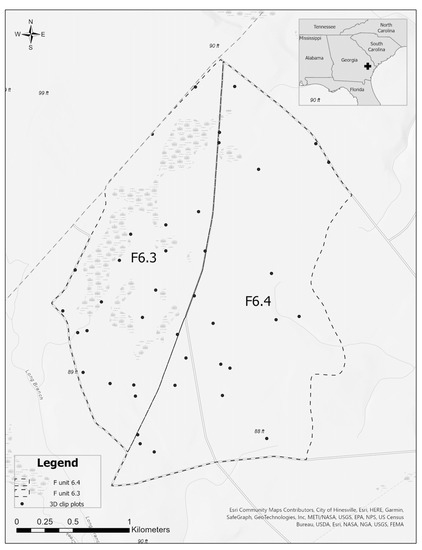
Figure 1.
Study area and sampling distribution of co-located TLS scans and vegetation and fuel biomass samples (n = 41). They were sampled before and after two prescribed burns.
Before each burn, vegetation and fuel categories were recorded in both the pre- and post- burn clip plots. Vegetation, fuel category and biomass data were collected using a simplified approach from Hawley et al. [30]. The sampling area was 0.5 m in width by 0.5 m in length by 1 m in height. The frame was subdivided into two vertical sampling layers or strata: ground to 30 cm and 30 to 100 cm. The vegetation and fuel categories for this site were defined as woody live vegetation, now dead woody vegetation, woody litter, woody dead and downed 1 h fuels, 10 h fuels, 100 h fuels, 1000 h fuels, pinecones, conifer litter, conifer needles, and herbaceous vegetation, which includes graminoids, forbs, and vines. The ‘now dead woody vegetation’ category was used only in post-burn sampling to classify pre-burn woody live stems that were partially consumed by the prescribed fire and when the aboveground plant was clearly dead or top-killed. There were no 1000 h fuels found in our plots. A detailed description of each vegetation and fuel category is in Appendix A. Before the burn, within both the pre- and post-burn plots, the presence and absence of each vegetation and fuel category were recorded within each stratum. At the pre-burn plot, the biomass was destructively harvested from each stratum. After the burn, within each post-burn clip plot, the presence and absence of each vegetation and the fuel category were recorded again and the biomass was destructively harvested within each stratum. In the Athens Prescribed Fire Science Laboratory, Athens, GA, USA, the biomass was sorted, dried, and weighed to determine the dry weight (in g m−2) of each vegetation and fuel category. The sorted biomass was dried at 70 °C until the weight of the sample no longer changed, typically within 48–72 h. Dry mass values are found in Appendix B.
2.3. Vegetation and Fuel Mass Classes
For this study, we used our aforementioned field-derived vegetation and fuel categories (Appendix A) to create the vegetation and fuel mass classes used for our linear modeling (Figure 2). This included total surface biomass (‘Total’), total without fine woody debris (‘Total no FWD’), total below 30 cm height (‘Total 0–30 cm’), fine vegetation and fuels only (‘Fine Fuels’), fine woody debris only (‘FWD’), and total below 30 cm height without FWD (‘Total 0–30 cm no FWD’). Total was the mass of all living and dead vegetative material. Total no FWD was the Total category minus any fine woody debris in the 10 h and 100 h fuel categories and pinecones. Total 0–30 cm was the total mass found under 30 cm in height. Fine Fuels included all grass, forb, and vine material (live and dead), dead leaves (pine and cypress needles, and broadleaves), other fine tree litter (bark flakes, reproductive organs: catkins, etc.), and 1 h fuels. The Total no FWD and Fine Fuels categories were created because coarse (1000 h) and fine woody debris (10,100 h) and live stems are rarely consumed, or only partially consumed in these systems [25], and fire practitioners often focus on “fine fuels” that are most available to burn during prescribed fire operations in the southeastern U.S. [59,60]. In fact, FWD was only 14% of the total mass, and there was no difference in FWD mass between the pre-burn (mean: 130.0 g m−2, std: 154.8 g m−2) and the post-burn (mean: 127.6 g m−2, std: 170.4 g m−2) samples (t-test, p = 0.92). The Total 0–30 cm category was created because most of the mass (95%) was found in this layer, and we wanted to test its predictive power compared to the entire area measured up to 100 cm. In the end, eight vegetation and fuel mass classes were created for our linear modeling (Figure 2). All pre-burn data were used for the first six classes (‘Total’, ‘Total no FWD’, ‘Total 0–30 cm’, ‘Fine Fuels’, ‘FWD’, ‘Total 0–30 cm no FWD’). The next two included the post-burn total surface biomass (‘Total 0–30 cm Post’) and the pre- and post-burn total surface biomass below 30 cm combined (‘Total 0–30 cm Pre and Post’).
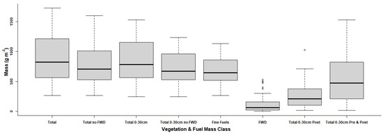
Figure 2.
Box plots of surface dry mass (g m−2) distinguished by our vegetation and fuel mass classes. All box plots include only pre-burn biomass data (n = 41), except for Total ‘0–30 cm Post’, which includes only post-burn data (n = 41) and ‘Total 0–30 cm Pre and Post’, which includes both pre- and post-burn data (n = 82). See text and Appendix A for fuel class and category descriptions.
2.4. Terrestrial Lidar Processing
For this study, we used the Leica BLK360 (Leica Geosystems, Heerbrugg, Switzerland) terrestrial laser scanner, deployed as described above and in Pokswinski et al. [45]. The BLK360 is particularly suited for use in forest mensuration applications because it is lightweight (1 kg), affordable (<$20 K), quick (<5 min per scan), is splash resistant and is a single-return laser. The area of coverage is 360° horizontally and 300° vertically. The laser has a wavelength of 830 nm, a beam divergence of 0.4 m rad, a range accuracy of 4 mm at a 10 m distance and of 7 mm at a 20 m distance, a maximum pulse rate of 360,000 points s−1, and a maximum range distance of 60 m [40]. The unit has multiple sampling density settings to control the number of points, which can help manage the data collection time and size. We used the medium density setting, which resulted in a scan time of less than four minutes.
From each single scan, a variety of metrics were calculated to summarize the point cloud and to serve as predictor variables for potential inclusion in the models. Prior to this, a series of pre-processing steps was applied. The scans were first exported from the sensor to PTX format using the Cyclone Register 360 (BLK Version) software (Leica Geosystems, Heerbrugg, Switzerland). This format retains all gap values, i.e., pulses that do not have an associated return [40]. The PTX point cloud was also converted to LAS format and clipped to a 15 m radius. Then, a distance-based noise filter was used to remove stray points in the point cloud. Next, the ground points were classified using a cloth simulation filter, where all ground points were normalized relative to the ground, and ground points were removed. The cloth simulation filter ground classification method classifies ground returns by modeling a rigidness-constrained cloth surface defined by an inverted point cloud [61].
A set of metrics were calculated from the PTX data to characterize the proportion of transmitted pulses that were returned. Within defined height bins (0.5, 1, 1.5, 2, >2 m) and using only the non-ground points in the normalized point cloud, summary metrics for the height measures were generated to characterize the central tendency and variability in the height measurements, including maximum and minimum height, mean and median height, skewness, and kurtosis. We also implemented a summarization method that was aimed at characterizing the areas of occlusion (i.e., all pulses are returned before reaching the current volume), which made use of spherical voxels and allowed us to estimate the proportion of pulses passing through a volume that is returned from that volume. Once this method was applied, summary metrics were generated from the results based on height strata, similar to the summarization process for the normalized data.
To generate additional metrics, the point cloud was also voxelized at an 8 cm3 spatial resolution. Trees were then segmented and stems were classified using the TreeLS package [62], and basal area, mean DBH, mean tree height, max tree height and canopy base height were calculated for all detected trees above 4 cm DBH. The points classified as “stem” were then removed from the point cloud and a surface vegetation and fuels point cloud was generated with the remaining points between 0 and 3 m in height. The surface vegetation point cloud was then filtered with the nearest neighbor values using the ‘fastpointmetrics’ function in TreeLS. These points were filtered using threshold values of linearity, verticality, planarity and a 2-dimensional eigenratio. The result was point clouds that contained points that represented a high probability of fine fuels or coarse woody debris.
In summary, this process resulted in 162 TLS metrics, broken down by (1) how the scan was divided or not [entire scan, by stratum (0.5, 1, 1.5, 2, >2 m), surface vegetation (0–3 m), classified fine and coarse woody debris (0–3 m)], (2) metric type (general, height statistic, quantiles, occlusion, trees), and (3) whether the metric used the point cloud or the voxelized point cloud. A detailed description of each metric is found in Appendix C.
2.5. Linear Modeling
We applied the leaps and bounds linear regression approach, using the leaps package [63] in the R Statistical Software (v4.0.2 [64]). This approach was originally developed by Furnival and Wilson [65], and was applied in the field of Forestry to test the linear relationships present in a large multivariate dataset using a parsimonious approach. It performs a comprehensive search for the best subsets of variables using a ‘branch-and-bound’ algorithm and a stopping rule to decide how many variables to use. If this linear regression approach proves useful, its application across similarly structured ecosystems would be less computationally expensive than more complex approaches (non-linear, polynomial, etc.). Linear models in R are developed using QR decomposition to solve for least squares.
Eight linear models were run using the vegetation and fuel mass classes as dependent variables and the 162 TLS metrics as independent variables. We used the ‘exhaustive’ method within the ‘subregs’ function, which performs an exhaustive approach on all combinations of variables given a target maximum subset size, which in this case, was six. A target of six was set because we wanted to optimize the number of dependent variables for model interpretability and computational efficiency, and to be able to continue cycling through all possible variable combinations. The six chosen variables were input variables to the ‘lm’ function in R to provide linear model output statistics, specifically, the R2, p-value, and RMSE for each model. Schwarz information criterion (BIC) [66] values were obtained from the ‘which.min’ function set for BIC generated in the ‘subregs’ function in the leaps package. Models were optimized to have low BIC values and to have the fewest variables.
Consumption was estimated using the Total 0–30 cm data. Observed consumption was calculated by subtracting the post-burn mass values < 30 cm in height from the pre-burn mass values < 30 m in height for each plot. Predicted consumption was calculated by subtracting the predicted mass values of the Total 0–30 cm post-burn linear model from the predicted mass values of the Total 0–30 cm pre-burn linear model for each plot. We applied a linear model using the ‘lm’ R package to assess the relationship between the observed and model predicted consumption values.
3. Results
From the leaps and bounds regression, all linear models were significant (p < 0.05), with an R2 ranging from of 0.65 to 0.74, when using a subset of six variables and the exhaustive method of variable selection (Table 1 and Table 2, Figure 3 and Figure 4, Appendix D). Using the pre-burn data, the best performing linear model was Total 0–30 cm (R2 = 0.74, BIC = −29), while the worst performing model was FWD (R2 = 0.61, BIC = −12, Table 1). The pre- and post-burn data combined also illustrated a significant linear model, with an R2 of 0.69. The models including the post burn data, either alone or combined with pre-burn data, did not perform as well as the pre-burn data alone; this is because there was less variation in the mass values post-burn. Similarly, this was also true for FWD (Figure 4b). Furthermore, the linear relationship between the observed and predicted consumption was significant (R2 = 0.70, p = 1.325 × 10⁻¹¹, Figure 3d).

Table 1.
Statistical results from leaps and bounds linear regression, which illustrate the resulting model selected subset of six TLS metrics used to predict the associated vegetation and fuel mass classes (linear models). All models had a df = 34, except Total 0–30 cm Pre and Post, which had df = 75. See Appendix C for a full list of metrics and their definitions. All models resulted in a p-value of <0.01.
Table 2.
Selected metrics from linear models illustrating the portion of the scan in which the metric was derived, the metric type, as well as the description of each metric. Stratum refers to the height layer within each scan in which the metric was derived, i.e., stratum 1: 0–0.5 m, 2: 0.5–1 m, 3: 1–1.5 m, 4: 1.5–2 m, and 5: >2 m. The numbers in parentheses refer to the number of times that particular metric was selected across the eight linear models in this study. Metric type refers to either a height statistic, general or standard TLS metric (e.g., point density), metric by quantiles, or identified tree structures within each scan. A more detailed description of all metrics is found in Appendix C.
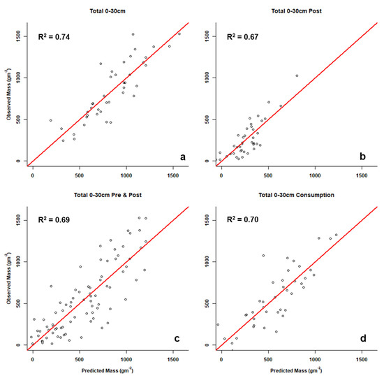
Figure 3.
Observed vs. predicted surface biomass for the Total 0–30 cm vegetation and fuel mass class, using the pre-burn ((a), n = 41), post-burn ((b), n = 41), pre- and post-burn combined (c), (n = 82), and consumption ((d), n = 41) linear models.
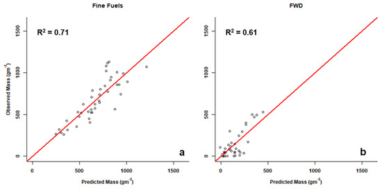
Figure 4.
Observed vs. predicted surface biomass comparing the fine fuels (a) and fine woody debris (b) vegetation and fuel mass classes and their respective linear models.
These eight linear models, with a possible 6 TLS metrics selected for each model, resulted in 48 total selected metrics, which were identified as being the most important when predicting mass (Table 1 and Table 2). Descriptions of the selected metrics are in Table 2, and all metric descriptions are in Appendix C. The metrics were all significant predictors (p < 0.05). Though the metrics were not explicit between models, there were some similarities found. In total, 33 unique metrics, or 20% of the (162 total) input TLS metrics, were selected among the eight models. In total, 30 (91% of 33) were from metrics calculated from different strata or height quantiles within each TLS scan. Of the remaining 3, 2 included the mean and standard deviation of heights in the entire scan. These 2 metrics were used in 5 of the eight models. The last one was a tree-metric: maximum tree height. This was only used once, in the Total 0–30cm Post model. There were 6 metrics associated with space and occlusion (of 37 total) selected within five models.
The selected metrics were identical for the Total and Total 0–30 cm models (Table 1). Three metrics for the Total no FWD and Fine Fuels models were similar: PD2 and % of PD2, representing the point density within 0.5–1 m of the height profile and the 65th quantile in height within the scan. The selected metrics were unique between the Total 0–30 cm and Total 0–30 cm Post models. The metrics were more mixed in the Total 0–30 cm Pre and Post model. This model had the largest range of metric types compared to the other models.
4. Discussion
This study represents a critical step for the operational application of single TLS methodology for measuring vegetation and fuel characteristics. We found that linear models can be used in frequently burned southeastern U.S. ecosystems to estimate fine-scale surface vegetation and fuel biomass using TLS vegetation metrics, and by predicting pre and post burn mass, they c-an estimate consumption. We also found that the first 95% of the total mass was found within the first 30 cm of the fuelbed and that using this value (e.g., Total 0–30 cm) produced the highest performing linear models (e.g., Total 0–30 cm, Table 1, Figure 3). This also includes estimating fine fuels, the largest proportion of mass pre-burn and mass consumed (Table 1, Figure 4a). FWD could also be estimated using this linear regression method (Figure 4b); however, we found that FWD represented 14% of the total mass, and, more importantly, that this was minimally reduced by the fire (i.e., no difference between pre- and post-burn FWD) and thus did not contribute significantly to overall consumption. These findings illustrate a simple and practical method for predicting fine-scale mass from TLS-derived metrics.
The strength of the models that we developed can be attributed to our sample size, the large range of surface mass and fuel types sampled, and the variation in consumption during the fires. Furthermore, the three-dimensional nature of the TLS scans created a dataset from which a comprehensive list of TLS metrics could be derived and used to predict a selection of surface fuel characteristics that are known to drive fire behavior. Across the eight linear models, 33 of 162 TLS metrics (20% of total) were selected to best predict surface biomass. The selected metrics between models corresponded similarly when the vegetation within each category was similar (e.g., Total vs. Total 0–30 cm). The metrics were unique between the Total 0–30 cm pre-burn and Total 0–30 cm post-burn models, illustrating the distinct representation of the surface vegetation structure before and after fire both within and across these scans. When combined (Total 0–30 cm pre and post burn model), the metrics were dispersed between the individual models (Total 0–30 cm vs. Total 0–30 cm post), where complex similarities across the pre- and post-burn scans represented a higher range of variability between the pre- and post-burn scans and associated biomass. Over 90% of the selected metrics (30 of 33) represented vegetation and space between vegetation in each scan’s height profile (Table 2, strata, quantiles, etc.), illustrating the profound complexity of vegetation at fine scales in these frequently burned systems. The 3 remaining metrics selected as important metrics were the mean and standard deviation height of the entire voxelized point cloud, as well as the max tree height. These 3 metrics were found in four models. Max tree height was only chosen in one model: the only post-scan model run (Total 0–30 cm Post). This illustrates the significance of characterizing the entire forest structure across the vertical and horizontal plane (hence using height profiles and quantiles, etc., Table 2) beyond only explicit tree measurements to model the variability in surface vegetation and fuel biomass. Furthermore, empty space in the scan data were partitioned as gaps in vegetation and gaps due to occlusion. This was represented in 37 TLS of the total 162 metrics, of which 6 were chosen within five linear models (Table 1 and Table 2). This illustrates the relevance of accounting for both true empty space and space that appears empty in scans but is an artifact of scan occlusion; these are all important factors when interpreting scan data and modeling surface biomass.
Given that surface fuel heterogeneity is complex and difficult to capture, the sensitivity of TLS is up to the task of capturing most of this fine-scale structural variation. Furthermore, our single-scan and linear modeling approach is relatively simple compared to other more direct one-to-one coupled methods. Other methods include linking fine-scale mass and volume of understory vegetation down to the 1.0 m3 and 6.25 × 10⁻² m3 scale [27,33]. These methods use high-resolution TLS instrumentation that requires extensive processing to merge several TLS scans together and manually crop out each 3D vegetation plot or individual plant from the resulting merged 3D point cloud. Though this does create a more ‘complete’ 3D image of the vegetation by reducing occlusion and enhancing realism, its practical utility for extensive and repeated sampling work, and management applications, remains questionable. Furthermore, this method is likely prone to error that is associated with directly linking field measurements and TLS data cropped to the 1000 cm3 (or 10 cm × 10 cm × 10 cm) scale; this is because both are performed manually and are impacted by, e.g., wind during scans, placement of scanner and sampling frame, and clipping biomass at 10 cm intervals. Our field and processing approach was distinct from these methods by acquiring and processing one TLS scan from a push button instrument in one location [45], then clipping in situ, drying, sorting, and weighing vegetation from only two strata (0–30, 30–100 cm), and running a linear regression technique that pulls out only a fraction (6 variables) of the TLS metrics to explain up to 74% of the variation in surface vegetation and fuel biomass. Even if we only measured total dry mass, without sorting into explicit vegetation and fuel categories, or even height categories (including FWD), our linear models still performed well (e.g., ‘Total’ category, R2 = 0.70, Table 1) and could be readily tested in other systems.
The TLS Instrument used in this study was useful because of its simple and non-bias push-button approach. It could, however, prove useful to test the relationship between metrics derived from other TLS instruments and surface biomass to expand this study’s applicability. For instance, there are other 360° scanners that have different frequencies and ranges [40]. There are mobile terrestrial scans that, while walking a transect for example, could collect and process a more complete 3D point cloud of vegetation structure by simultaneously eliminating the merging process required for stationary TLS scans and reducing issues of occlusion. However, compared to our single-scan approach, these mobile scanners are currently more expensive, more difficult to operate, and the quality of the point cloud is dependent on the pace and path taken by the user, which limits replicability [35]. This single-scan approach can be repeated in the same plot, as we did for consumption, for long-term consistent data collection with minimal bias.
Creating TLS-derived models that estimate variation in surface biomass within forested stands paves the way for creating realistic inputs and robust test datasets for spatially explicit fire behavior models [6]. These data are particularly useful in ecosystems that are dominated by fine-scale surface fuels [22] and used as inputs into high-resolution coupled fire–atmosphere models that operate in three dimensions with the ability to represent within-stand variability [8,9,67]. Such a high-resolution representation of fuel variation will improve our prediction of heterogeneity in fire effects and the underlying physical influences of vegetation on the fire environment [13]. In this study, we found that the variability in surface mass across these two burn units (658 ha total) was considerable [mean: 841 g m−2, stdev: 350 g m−2 from the ‘Total 0–30’ model (Figure 2)], highlighting the need to think beyond stand-level averages [68]. Consumption followed this same trend (mean: 580 g m−2, std: 353 g m−2), allowing for connections between energy-released-by-fire and fire effects [69]. Both results demonstrate the ability of this method to represent 3D variability in mass and consumption across a stand, as well as the significance of low (here <30 cm) vegetation, particularly fine fuels, when fine to coarse wood consumption is negligible. As such, we recommend that these TLS data for pre-burn biomass estimates be used as inputs to coupled fire–atmosphere models, while our consumption estimates can be compared to model outputs.
This single-scan sampling technique was designed to be simple and efficient, specifically for long-term monitoring [45]. Each scan captures a high-resolution 3D image of a plot that can be analyzed repeatedly as new analyses and metrics are developed with minimal to no post-processing. Incorporating surface biomass estimation into this approach is critical, particularly for frequently burned ecosystems in which mass varies at fine scales, and influences fire behavior and effects at these same scales [15]. Broader stand-level averages do not account for this fine-scale heterogeneity and are not sufficient for coupling to fire–atmosphere models and predicting fire effects [10,70]. This approach can add more explicit estimates of mass to existing broad-scale approaches, such as ecosystem-level photo-load series and custom fuel models [12,71]. The benefit for management, especially if preliminary dry mass values have been incorporated, is that scans can be taken efficiently within vegetation types of interest and run through the established linear models to provide information on the explicit variability in surface biomass found within and across stands. Surface mass can be quite variable across stands, even within the same ecosystem type (e.g., longleaf pine Flatwoods vs. sandhills) based on fire histories, the time since fire, management practices, and general site characteristics (soil, overstory density, etc.). This approach could be used to monitor the effects of fire when associated with the detection of changes in the surface biomass, both before and after a fire, and to monitor the long-term restoration and maintenance of target surface fuel characteristics over time.
Future work for this study should be relevant to similar sites and other frequently burned ecosystems. The extension of these models will require testing across other regional longleaf pine forests or frequently burned ecosystems in other regions. We expect similarities in ecosystems with comparable physiognomy, though model-selected TLS metrics may vary depending on local factors, such as dominant trees, understory and site characteristics (e.g., soil, elevation, topography, climate, management). Validation procedures are needed to confirm their utility in the prediction of the fine-scale variability found in surface mass when they are used for fire behavior research, particularly using these fuels predictions coupled with site characteristics to create 3D surface fuel maps. Machine learning approaches could prove useful, especially as our sample size increases across ecosystems. Coupling these TLS-derived surface fuel biomass methods with airborne laser scanning could provide full spatially explicit vegetation distribution information across a given site.
5. Conclusions
In conclusion, this study illustrates an approach to expanding the utility of single-location terrestrial laser scanning for use in prescribed fire management and monitor the effects of fire, all benefitting from robust estimates of surface vegetation and fuel biomass. This study demonstrates the capability of simple TLS methods to measure within and across-stand variability, as well as estimated consumption. Lastly, these data and the linear models presented here could prove useful for deriving inputs to and validating outputs from coupled fire–atmosphere models, particularly for prescribed fire research and management.
Author Contributions
Conceptualization, E.L.L., S.P., A.M., M.R.G., N.S.S. and J.K.H.; methodology, E.L.L., S.P., C.M.H., A.M., M.R.G., N.S.S. and J.K.H.; formal analysis, E.L.L. and S.P.; investigation, E.L.L., S.P. and C.M.H.; resources, E.L.L., S.P. and C.M.H.; data curation, C.M.H. and E.L.L.; writing—original draft preparation, E.L.L.; writing—review and editing, E.L.L., S.P., C.M.H., A.M., M.R.G., N.S.S., A.T.H., C.H. and J.K.H.; visualization, E.L.L. and S.P.; project administration, E.L.L., S.P. and C.M.H.; funding acquisition, E.L.L., S.P., C.M.H., A.M., M.R.G., N.S.S., A.T.H., C.H. and J.K.H. All authors have read and agreed to the published version of the manuscript.
Funding
This research was funded by the Department of Defense, Strategic Environmental and Research Development Program, grant number RC19-1119 and RC20-1346, and Department of Defense, Environmental Security Technology Certification Program, grant number RC20-7189.
Institutional Review Board Statement
Not applicable.
Informed Consent Statement
Not applicable.
Data Availability Statement
Biomass data used in this study are available in the Appendix A, Appendix B, Appendix C and Appendix D.
Acknowledgments
We acknowledge the Department of Defense’s Strategic Environmental and Research Development Program, and the Environmental Security Technology Certification Program, particularly the Integrated Research Management Team, with special thanks to James Furman for his profound leadership. We give an extra special thanks to the Ft. Stewart Natural Resources and Forestry Staff, led by Bryan Whitmore. They illustrated exemplary support during this field campaign, particularly in facilitating the safety of our field crew, field support, and executing the experimental burns with extreme professionalism and efficiency. We thank the United States Department of Agriculture Forest Service Southern Research Station, Northern Research Station, and Rocky Mountain Research Station. We thank Tall Timbers Research Station for their support of technical staff. We thank field preparation, sampling and laboratory efforts provided by Derek Wallace, C. Wade Ross, Greg Chapman, Vanessa Niemczyk, Jacob Ney, Irenee Payne, and Quinn Hiers. The findings and conclusions in this publication are those of the authors and should not be construed to represent any official USDA or U.S. Government determination or policy.
Conflicts of Interest
The authors declare no conflict of interest.
Appendix A
Table of original vegetation and fuel categories collected in the field and their descriptions.
| Vegetation or Fuel Category | Description |
|---|---|
| Woody Live | Live material from evergreen and deciduous broadleaf shrubs or trees aboveground (i.e., stems, leaves, flowers, buds, etc.) |
| Now Dead Woody Vegetation | Only in post-burn sampling to classify pre-burn woody live stems that were partially consumed by the prescribed fire and the aboveground plant was clearly dead (aka top-killed) |
| Woody Litter | Downed leaf and litter material from evergreen and deciduous broadleaf shrubs or trees detached from its source (i.e., leaves, flowers, buds, etc.) |
| 1 h | Downed dead branches, twigs, and other small woody pieces that are severed from their original source of growth, and dead woody species that is still standing and attached to the ground and is less than 0.25 inch (0.64 cm) in diameter |
| 10 h | Downed, dead branches, twigs, and other small woody pieces that are severed from their original source of growth, female cones (i.e., megastrobilus, seed cone, or ovulate cone) from non-Pinus species, and dead woody species that are still standing and attached to the ground and is 0.25 inch to 1.0 inch (0.64 to 2.54 cm) in diameter |
| 100 h | Downed, dead tree and shrub boles, large limbs, and other woody pieces that are severed from their original source of growth and dead woody species that is still standing and attached to the ground and is 1.0 inch to 3.0 inch (2.54 to 7.6 cm) in diameter |
| 1000 h | Downed, dead tree and shrub boles, large limbs, and other woody pieces that are severed from their original source of growth and is 3.0 inch to 8 inch (7.6 cm to 20.3 cm) in diameter. Note that no 1000 h fuels were found in our plots for this study. |
| Pinecones | Intact female cones (i.e., megastrobilus, seed cone, or ovulate cone) from Pinus species |
| Conifer Litter | Needle from conifers other than Pinus species and downed woody material from conifer species that is too small to fit into the 1-h fuel category (ex: paper-thin pieces of bark, male pollen cones (aka microstrobilus), and pinecone fragments) |
| Pine Needles | Downed needles from Pinus species with long or short needles |
| Fine Vegetation | Live and dead material from bunchgrass species, wiregrass species, other graminoids, forbs, vines, and conifer seedlings |
Appendix B
Surface biomass values (g m−2) for each plot (row, n = 41) corresponding to the vegetation and fuel mass classes (headings) used in this study and described in the text. All values represent biomass found before the fire (pre-burn), except for the last column (Total 0–30 cm Post), which is the biomass measured after the fire in the post-burn plots. ‘Total 0–30 cm’ and ‘Total 0–30 cm Post’ classes were combined (n = 82) to produce the ‘Total 0–30 cm Pre and Post’ category (not shown here).
| Total | Total No. FWD | Total 0–30 cm | Total 0–30 cm No. FWD | Fine Fuels | FWD | Total 0–30 cm Post |
|---|---|---|---|---|---|---|
| 318.6 | 278.2 | 318.6 | 278.2 | 278.2 | 40.4 | 84.08 |
| 1124.92 | 1011.4 | 1075.04 | 961.52 | 945.96 | 113.52 | 178.92 |
| 470.16 | 432.36 | 466.08 | 428.28 | 404.44 | 37.8 | 43.52 |
| 942 | 854.8 | 942 | 854.8 | 854.8 | 87.2 | 101.12 |
| 787.68 | 787.68 | 782.2 | 782.2 | 787.68 | 0 | 16.76 |
| 490.68 | 472.96 | 490.68 | 472.96 | 472.96 | 17.72 | 95.16 |
| 553.2 | 531.76 | 550.32 | 528.88 | 521.68 | 21.44 | 23.84 |
| 565.28 | 320.72 | 565.28 | 320.72 | 320.72 | 244.56 | 110.4 |
| 622.16 | 533.24 | 618.72 | 529.8 | 521.96 | 88.92 | 219.12 |
| 739.16 | 725.88 | 685.72 | 672.44 | 555.36 | 13.28 | 169.84 |
| 1396.52 | 1020.12 | 1341.52 | 965.12 | 911.12 | 376.4 | 57.64 |
| 529.08 | 529.08 | 529.08 | 529.08 | 527.24 | 0 | 507.92 |
| 853.08 | 848.04 | 783.64 | 778.6 | 739.48 | 5.04 | 46.16 |
| 1122.36 | 630.76 | 1007.96 | 516.36 | 449.56 | 491.6 | 310.08 |
| 1373.76 | 876.28 | 1373.76 | 876.28 | 856.16 | 497.48 | 92.8 |
| 1318.32 | 1281.68 | 1150.44 | 1113.8 | 1003.8 | 36.64 | 207.16 |
| 1727.36 | 1434.68 | 1526.12 | 1233.44 | 1077.72 | 292.68 | 201.56 |
| 1648 | 1600.6 | 1256.72 | 1209.32 | 1020.44 | 47.4 | 213.04 |
| 467.52 | 406.36 | 461.44 | 400.28 | 353.04 | 61.16 | 302.6 |
| 1178.92 | 1131.12 | 1167.08 | 1119.28 | 1131.12 | 47.8 | 91.6 |
| 1276.64 | 806.28 | 1188.64 | 718.28 | 621.92 | 470.36 | 414.28 |
| 756.2 | 620.32 | 702.24 | 566.36 | 620.32 | 135.88 | 129.8 |
| 1512.44 | 983.6 | 1378.16 | 849.32 | 772.16 | 528.84 | 1027.36 |
| 434.6 | 434.6 | 434.6 | 434.6 | 423.52 | 0 | 122.16 |
| 591.92 | 527.72 | 591.92 | 527.72 | 516.24 | 64.2 | 386.96 |
| 266.16 | 266.16 | 243.44 | 243.44 | 266.16 | 0 | 165.04 |
| 913.56 | 612.6 | 900 | 599.04 | 564.56 | 300.96 | 483.2 |
| 694.28 | 642.32 | 693.24 | 641.28 | 642.32 | 51.96 | 332.16 |
| 881.68 | 737.24 | 881.68 | 737.24 | 737.24 | 144.44 | 661.72 |
| 495.8 | 495.8 | 389.88 | 389.88 | 314.28 | 0 | 146 |
| 614.36 | 572.28 | 586.64 | 544.56 | 572.28 | 42.08 | 224.88 |
| 820.84 | 660.92 | 820.84 | 660.92 | 660.92 | 159.92 | 205.64 |
| 707.52 | 707.52 | 707.52 | 707.52 | 707.52 | 0 | 15.4 |
| 1575.24 | 1175.08 | 1520.8 | 1120.64 | 1114.44 | 400.16 | 512.4 |
| 1217.8 | 1197.28 | 1033.44 | 1012.92 | 800.76 | 20.52 | 279.44 |
| 1244.08 | 1074.24 | 1244.08 | 1074.24 | 1068.6 | 169.84 | 442.52 |
| 1212.76 | 1123 | 1185.44 | 1095.68 | 988.28 | 89.76 | 282.24 |
| 1134.36 | 1060.12 | 1037.4 | 963.16 | 842.68 | 74.24 | 378.04 |
| 938.92 | 889.4 | 938.92 | 889.4 | 889.4 | 49.52 | 544.56 |
| 639.04 | 531.76 | 639.04 | 531.76 | 531.76 | 107.28 | 709.2 |
| 264.04 | 264.04 | 264.04 | 264.04 | 261.72 | 0 | 190.8 |
Appendix C
The 162 TLS metrics used in the linear models for this study. The gray rows are those chosen in our regression models for this study; see Table 1. These illustrate from which portion of the scan the metric was derived, the metric type, as well as a description of each metric. Stratum refers to the height layer within each scan in which the metric was derived, i.e., strata 1: 0–0.5 m, 2: 0.5–1 m, 3: 1–1.5 m, 4: 1.5–2 m, and 5: >2 m. ‘Metric type’ refers to either a height statistic, general or standard TLS metric (e.g., point density), metric associated with space and occlusion of TLS points within the scan (e.g., true empty space, occlusion by trees), metric by height quantiles, or identified tree structure within each scan. Metrics were calculated from either the point cloud or the voxelization of the point cloud to 2 cm × 2 cm × 2 cm voxels. “Standardized” means that the point cloud was voxelized before the metric was calculated. Standardized surface fuels means that identified tree stems were removed before the voxelization of each point cloud below 3 m in height. All scans were normalized to account for topographic variation and cropped to a 15 m radius from the center before any metric calculation. Triangular Greenness Index (TGI) = ((Green − 0.39) * (Red − 0.61)) * Blue values extracted from the BLK camera. Visible Atmospherically Resistant Index (VWRI) = (Green − Red)(Green + Red − Blue) extracted from the BLK camera. See text for more details of the methodology.
| Portion of Scan | Metric Type | Voxelized/Point Cloud | No. of Metrics | Metric | Description |
|---|---|---|---|---|---|
| By stratum | General | Point Cloud | 5 | PD (1 to 5), e.g., PD1 | Point density (PD) in strata 1 to 5 |
| By stratum | General | Point Cloud | 5 | % PD (1 to 5) | % of points in strata 1 to 5 |
| By stratum | General | Point Cloud | 5 | TGI (1 to 5) | Triangular Greenness Index (TGI) in strata 1 to 5 |
| By stratum | General | Point Cloud | 5 | VARI (1 to 5) | Visual Atmospheric Resistance Index (VARI) in strata 1 to 5 |
| By stratum | Height statistic | Point Cloud | 5 | Mean Ht (1 to 5) | Mean height (Ht) in strata 1 to 5 |
| By stratum | Height statistic | Point Cloud | 5 | Median Ht (1 to 5) | Median height in strata 1 to 5 |
| By stratum | Height statistic | Point Cloud | 5 | SD Ht (1 to 5) | Standard deviation (SD) of heights in strata 1 to 5 |
| By stratum | Height statistic | Point Cloud | 5 | Sk Ht (1 to 5) | Skewness of heights (Sk) in strata 1 to 5 |
| By stratum | Height statistic | Point Cloud | 5 | Ku Ht (1 to 5) | Kurtosis (Ku) of heights in strata 1 to 5 |
| By stratum | Space and Occlusion | Point Cloud | 5 | % Occluded (1 to 5) | % of non-ground points occluded in strata 1 to 5 |
| By stratum | Space and Occlusion | Point Cloud | 5 | % Space (1 to 5) | % of unreturned non-ground points (true empty space) in strata 1 to 5 |
| By stratum | Space and Occlusion | Point Cloud | 5 | Mean Prop Non-occluded (1 to 5) | Mean proportion(Prop) of occluded and no returns in strata 1 to 5 |
| By stratum | Space and Occlusion | Point Cloud | 5 | SD Prop Non-occluded (1 to 5) | SD of proportion of occluded and no returns in strata 1 to 5 |
| By stratum | Space and Occlusion | Point Cloud | 5 | Sk Prop Non-occluded (1 to 5) | Sk of proportion of occluded and no returns in strata 1 to 5 |
| By stratum | Space and Occlusion | Point Cloud | 5 | Ku Prop Non-occluded (1 to 5) | Ku of proportion of occluded and no returns in strata 1 to 5 |
| 0–3 m | General | Voxelized | 2 | PD CWD (10 or 1000) | Standardized surface fuel PD classified as 1–10 h or 100–1000 h fuels |
| 0–3 m | General | Voxelized | 2 | TDI CWD (10 or 1000) | Standardized surface fuel TDI classified as 1–10 h or 100–1000 h fuels |
| 0–3 m | General | Voxelized | 2 | VARI CWD (10 or 1000) | Standardized surface fuel VARI classified as 1–10 h or 100–1000 h fuels |
| 0–3 m | Height statistic | Voxelized | 2 | Mean CWD (10 or 1000) | Standardized surface fuel mean height classified as 1–10 h or 100–1000 h fuels |
| 0–3 m | Height statistic | Voxelized | 2 | Median CWD (10 or 1000) | Standardized surface fuel median height classified as 1–10 h or 100–1000 h fuels |
| 0–3 m | Height statistic | Voxelized | 2 | SD CWD (10 or 1000) | Standardized surface fuel SD of height classified as 1–10 h or 100–1000 h fuels |
| 0–3 m | Height statistic | Voxelized | 2 | Sk CWD (10 or 1000) | Standardized surface fuel Sk of height classified as 1–10 h or 100–1000 h fuels |
| 0–3 m | Height statistic | Voxelized | 2 | Ku CWD (10 or 1000) | Standardized surface fuel Ku of height classified as 1–10 h or 100–1000 h fuels |
| Entire scan | General | Point Cloud | 1 | Ground PD | Number of TLS points classified as ground |
| Entire scan | General | Point Cloud | 1 | Veg PD | Number of TLS points not classified as ground |
| Entire scan | General | Point Cloud | 1 | % Ground | % of points classified as ground |
| Entire scan | General | Point Cloud | 1 | TGI | TGI |
| Entire scan | General | Point Cloud | 1 | VARI | VARI |
| Entire scan | General | Point Cloud | 1 | % Above Mean Ht | % of non-ground points above mean height |
| Entire scan | General | Point Cloud | 1 | % Above 2SD Mean Ht | % of non-ground points 2SD above mean height |
| Entire scan | General | Voxelized | 1 | Total Volume | PD of standardized point cloud |
| Entire scan | General | Voxelized | 1 | TGI Voxels | TGI of standardized point cloud |
| Entire scan | General | Voxelized | 1 | VARI Voxels | VARI of standardized point cloud |
| Entire scan | Height statistic | Point Cloud | 1 | Maximum Ht | Maximum height of TLS points in the entire scan |
| Entire scan | Height statistic | Point Cloud | 1 | Mean Ht | Mean height of TLS points in the entire scan |
| Entire scan | Height statistic | Point Cloud | 1 | SD Ht | SD of TLS point heights in the entire scan |
| Entire scan | Height statistic | Point Cloud | 1 | Sk Ht | Sk of TLS point heights in the entire scan |
| Entire scan | Height statistic | Point Cloud | 1 | Ku Ht | Ku of TLS point heights in the entire scan |
| Entire scan | Height statistic | Voxelized | 1 | Mean Ht Voxels | Mean height of standardized point cloud |
| Entire scan | Height statistic | Voxelized | 1 | Median Ht Voxels | Median height of standardized point cloud |
| Entire scan | Height statistic | Voxelized | 1 | SD Ht Voxels | SD of heights in standardized point cloud |
| Entire scan | Height statistic | Voxelized | 1 | Sk Ht Voxels | Sk of heights in standardized point cloud |
| Entire scan | Height statistic | Voxelized | 1 | Ku Ht Voxels | Ku of heights in standardized point cloud |
| Entire scan | Space and Occlusion | Point Cloud | 1 | % Total Unreturned Points | % of unreturned points overall |
| Entire scan | Space and Occlusion | Point Cloud | 1 | % Area Occluded Points | % of possible non-ground points from occluded |
| Entire scan | Space and Occlusion | Point Cloud | 1 | % True Open Space | % of unreturned non-ground points (true empty space) |
| Entire scan | Space and Occlusion | Point Cloud | 1 | Mean Prop Non-occluded | Mean proportion of true points that are not occluded |
| Entire scan | Space and Occlusion | Point Cloud | 1 | SD Prop Non-occluded | SD of proportion of occluded and no returns in entire scan |
| Entire scan | Space and Occlusion | Point Cloud | 1 | Sk Prop Non-occluded | Sk of proportion of occluded and no returns in entire scan |
| Entire scan | Space and Occlusion | Point Cloud | 1 | Ku Prop Non-occluded | Ku of proportion of occluded and no returns in entire scan |
| Entire scan | Quantiles | Point Cloud | 19 | Ht 5th Q to Ht 95th Q | Height at 5th to 95th quantiles in intervals of 5 |
| Entire scan | Quantiles | Point Cloud | 9 | % PD 10th Q to % PD 90th Q | % of points below 10th to 90th quantile of max ht in intervals of 10 |
| Entire scan | Trees | Voxelized | 1 | Total BA | Total basal area |
| Entire scan | Trees | Voxelized | 1 | Mean BA | Mean basal area |
| Entire scan | Trees | Voxelized | 1 | Mean Tree Ht | Mean tree height |
| Entire scan | Trees | Voxelized | 1 | Mean DBH | Mean diameter at breast height (DBH) of all detected trees > 4 cm DBH |
| Entire scan | Trees | Voxelized | 1 | No. Trees | Number of trees detected |
| Entire scan | Trees | Voxelized | 1 | Max Tree Ht | Maximum tree height |
| Entire scan | Trees | Voxelized | 1 | SD Tree Hts | SD of tree heights |
| Entire scan | Trees | Voxelized | 1 | Mean Canopy Base Ht | Mean tree canopy base height |
| 0–3 m | General | Voxelized | 1 | Surface VD | Standardized surface fuel VD |
| 0–3 m | General | Voxelized | 1 | Surface TGI | Standardized surface fuel TGI |
| 0–3 m | General | Voxelized | 1 | Surface VARI | Standardized surface fueVARI |
| 0–3 m | Height statistic | Voxelized | 1 | Surface Mean Ht | Standardized surface fuel mean height |
| 0–3 m | Height statistic | Voxelized | 1 | Surface Median Ht | Standardized surface fuel median height |
| 0–3 m | Height statistic | Voxelized | 1 | Surface SD ht | Standardized surface fuel SD of height |
| 0–3 m | Height statistic | Voxelized | 1 | Surface Sk ht | Standardized surface fuel Sk of height |
| 0–3 m | Height statistic | Voxelized | 1 | Surface Ku ht | Standardized surface fuel Ku of height |
Appendix D
Raw statistical outputs (from R) of the eight linear regression models, in order as shown in Figure 2 and Table 1.
| Linear Model “Total”: | ||||
| Call: | ||||
| lm(formula = focus_predictor[, 1] ~ h_l2_per + s_l2_prop_sk + s_l2_prop_ku + s_l5_zero_per + vox_l1_mean + fuel0_3l1_cnt, data = coef) | ||||
| Residuals: | ||||
| Min | 1Q | Median | 3Q | Max |
| −109.59 | −26.96 | −10.31 | 15.90 | 134.81 |
| Coefficients: | ||||
| Estimate | Std. Error | t value | Pr(>|t|) | |
| (Intercept) | −3.300 × 10³ | 8.601 × 10² | −3.837 | 0.000516 *** |
| h_l2_per | −1.093 × 101 | 2.386 × 100 | −4.581 | 5.97 × 10⁻⁵ *** |
| s_l2_prop_sk | −5.363 × 101 | 9.818 × 100 | −5.462 | 4.31 × 10⁻⁶ *** |
| s_l2_prop_ku | 1.673 × 100 | 2.906 × 10⁻¹ | 5.757 | 1.78 × 10⁻⁶ *** |
| s_l5_zero_per | 3.379 × 101 | 8.947 × 100 | 3.777 | 0.000611 *** |
| vox_l1_mean | 6.566 × 101 | 9.710 × 100 | 6.762 | 8.99 × 10⁻⁸ *** |
| fuel0_3l1_cnt | 1.522 × 10⁻⁴ | 3.072 × 10⁻⁵ | 4.954 | 1.97 × 10⁻⁵ *** |
| --- | ||||
| Signif. codes: 0 ‘***’ | ||||
| Residual standard error: 57.33 on 34 degrees of freedom | ||||
| Multiple R-squared: 0.7167, | Adjusted R-squared: 0.6668 | |||
| F-statistic: 14.34 on 6 and 34 DF, | p-value: 4.464 × 10⁻⁸ | |||
| Linear Model “Total no FWD”: | ||||
| Call: | ||||
| lm(formula = focus_predictor[, 1] ~ h_l2_cnt + h_l2_per + h_l5_cnt + h_zq65 + s_l1_prop_ku + s_l3_zero_per, data = coef) | ||||
| Residuals: | ||||
| Min | 1Q | Median | 3Q | Max |
| −76.143 | −32.682 | 1.856 | 17.751 | 154.496 |
| Coefficients: | ||||
| Estimate | Std. Error | t value | Pr(>|t|) | |
| (Intercept) | 1.730 × 10³ | 4.161 × 10² | 4.158 | 0.000206 *** |
| h_l2_cnt | 1.567 × 10⁻³ | 2.869 × 10⁻⁴ | 5.463 | 4.30 × 10⁻⁶ *** |
| h_l2_per | −5.622 × 101 | 1.114 × 101 | −5.048 | 1.49 × 10⁻⁵ *** |
| h_l5_cnt | −1.591 × 10⁻⁴ | 3.570 × 10⁻⁵ | −4.457 | 8.60 × 10⁻⁵ *** |
| h_zq65 | 1.821 × 101 | 3.136 × 100 | 5.806 | 1.54 × 10⁻⁶ *** |
| s_l1_prop_ku | 6.610 × 10⁻¹ | 1.810 × 10⁻¹ | 3.651 | 0.000869 *** |
| s_l3_zero_per | −1.585 × 101 | 4.304 × 100 | −3.683 | 0.000796 *** |
| --- | ||||
| Signif. codes: 0 ‘***’ | ||||
| Residual standard error: 52.38 on 34 degrees of freedom | ||||
| Multiple R-squared: 0.6509, | Adjusted R-squared: 0.5893 | |||
| F-statistic: 10.57 on 6 and 34 DF, | p-value: 1.306 × 10⁻⁶ | |||
| Linear Model “Total 0–30 cm”: | ||||
| Call: | ||||
| lm(formula = focus_predictor[, 1] ~ h_l2_per + s_l2_prop_sk + s_l2_prop_ku + s_l5_zero_per + vox_l1_mean + fuel0_3l1_cnt, data = coef) | ||||
| Residuals: | ||||
| Min | 1Q | Median | 3Q | Max |
| −92.231 | −26.795 | −8.902 | 20.862 | 113.172 |
| Coefficients: | ||||
| Estimate | Std. Error | t value | Pr(>|t|) | |
| (Intercept) | −2.903 × 10³ | 7.364 × 10² | −3.942 | 0.000383 *** |
| h_l2_per | −1.063 × 101 | 2.043 × 100 | −5.202 | 9.41 × 10⁻⁶ *** |
| s_l2_prop_sk | −4.573 × 101 | 8.406 × 100 | −5.440 | 4.60 × 10⁻⁶ *** |
| s_l2_prop_ku | 1.406 × 100 | 2.488 × 10⁻¹ | 5.652 | 2.44 × 10⁻⁶ *** |
| s_l5_zero_per | 2.966 × 101 | 7.660 × 100 | 3.872 | 0.000466 *** |
| vox_l1_mean | 6.107 × 101 | 8.313 × 100 | 7.346 | 1.64 × 10⁻⁸ *** |
| fuel0_3l1_cnt | 1.325 × 10⁻⁴ | 2.630 × 10⁻⁵ | 5.039 | 1.53 × 10⁻⁵ *** |
| --- | ||||
| Signif. codes: 0 ‘***’ | ||||
| Residual standard error: 49.09 on 34 degrees of freedom | ||||
| Multiple R-squared: 0.7388, | Adjusted R-squared: 0.6927 | |||
| F-statistic: 16.03 on 6 and 34 DF, | p-value: 1.191 × 10⁻⁸ | |||
| Linear Model “Total 0–30 cm no FWD”: | ||||
| Call: | ||||
| lm(formula = focus_predictor[, 1] ~ h_zq90 + h_zpcum3 + s_l1_prop_ku + s_l2_prop_sd + vox_l1_std + h100_1000_l1_kurt, data = coef) | ||||
| Residuals: | ||||
| Min | 1Q | Median | 3Q | Max |
| −108.20 | −20.29 | −4.60 | 23.29 | 70.88 |
| Coefficients: | ||||
| Estimate | Std. Error | t value | Pr(>|t|) | |
| (Intercept) | 62.0884 | 78.1550 | 0.794 | 0.43246 |
| h_zq90 | −41.8273 | 9.2926 | −4.501 | 7.54 × 10⁻⁵ *** |
| h_zpcum3 | −5.3703 | 0.9913 | −5.418 | 4.93 × 10⁻⁶ *** |
| s_l1_prop_ku | 0.7080 | 0.1559 | 4.542 | 6.68 × 10⁻⁵ *** |
| s_l2_prop_sd | 5.1922 | 1.0570 | 4.912 | 2.23 × 10⁻⁵ *** |
| vox_l1_std | 134.6971 | 23.2959 | 5.782 | 1.65 × 10⁻⁶ *** |
| hr100_1000_l1_kurt | 5.9487 | 1.7120 | 3.475 | 0.00142 ** |
| --- | ||||
| Signif. codes: 0 ‘***’ 0.001 ‘**’ | ||||
| Residual standard error: 42.04 on 34 degrees of freedom | ||||
| Multiple R-squared: 0.693, | Adjusted R-squared: 0.6389 | |||
| F-statistic: 12.79 on 6 and 34 DF, | p-value: 1.646 × 10⁻⁷ | |||
| Linear Model “FWD”: | ||||
| Call: | ||||
| lm(formula = focus_predictor[, 1] ~ h_l2_std + h_l2_skew + h_l5_std + h_zq90 + s_l5_zero_per + vox_l1_mean, data = coef) | ||||
| Residuals: | ||||
| Min | 1Q | Median | 3Q | Max |
| −51.358 | −17.052 | 0.497 | 16.804 | 51.966 |
| Coefficients: | ||||
| Estimate | Std. Error | t value | Pr(>|t|) | |
| (Intercept) | −2111.760 | 440.337 | −4.796 | 3.16 × 10⁻⁵ *** |
| h_l2_std | 4973.248 | 836.842 | 5.943 | 1.02 × 10⁻⁶ *** |
| h_l2_skew | 142.621 | 24.245 | 5.882 | 1.22 × 10⁻⁶ *** |
| h_l5_std | 55.306 | 15.496 | 3.569 | 0.001092 ** |
| h_zq90 | −24.575 | 7.321 | −3.357 | 0.001951 ** |
| s_l5_zero_per | 13.728 | 3.980 | 3.449 | 0.001519 ** |
| vox_l1_mean | 33.299 | 8.331 | 3.997 | 0.000326 *** |
| --- | ||||
| Signif. codes: 0 ‘***’ 0.001 ‘**’ 0.01 | ||||
| Residual standard error: 26.99 on 34 degrees of freedom | ||||
| Multiple R-squared: 0.6064, | Adjusted R-squared: 0.537 | |||
| F-statistic: 8.732 on 6 and 34 DF, | p-value: 8.808 × 10⁻⁶ | |||
| Linear Model “Fine Fuels”: | ||||
| Call: | ||||
| lm(formula = focus_predictor[, 1] ~ h_l2_cnt + h_l2_per + h_zq30 + h_zq65 + h_zpcum1 + h_zpcum6, data = coef) | ||||
| Residuals: | ||||
| Min | 1Q | Median | 3Q | Max |
| −77.99 | −17.87 | −6.53 | 19.78 | 79.50 |
| Coefficients: | ||||
| Estimate | Std. Error | t value | Pr(>|t|) | |
| (Intercept) | 9.332 × 101 | 1.525 × 10² | 0.612 | 0.544687 |
| h_l2_cnt | 7.504 × 10⁻⁴ | 1.473 × 10⁻⁴ | 5.094 | 1.30 × 10⁻⁵ *** |
| h_l2_per | −3.065 × 101 | 5.777 × 100 | −5.305 | 6.89 × 10⁻⁶ *** |
| h_zq30 | 5.573 × 101 | 1.226 × 101 | 4.546 | 6.60 × 10⁻⁵ *** |
| h_zq65 | 1.257 × 101 | 3.383 × 100 | 3.716 | 0.000725 *** |
| h_zpcum1 | 6.512 × 100 | 1.534 × 100 | 4.245 | 0.000160 *** |
| h_zpcum6 | −4.474 × 100 | 1.111 × 100 | −4.025 | 0.000301 *** |
| -- | ||||
| Signif. codes: 0 ‘***’ 0.001 | ||||
| Residual standard error: 37.11 on 34 degrees of freedom | ||||
| Multiple R-squared: 0.7119, | Adjusted R-squared: 0.661 | |||
| F-statistic: 14 on 6 and 34 DF, | p-value: 5.892 × 10⁻⁸ | |||
| Linear Model “Total 0–30 cm Post”: | ||||
| Call: | ||||
| lm(formula = focus_predictor[, 1] ~ h_zq45 + h_zpcum8 + h_zpcum9 + MaxTH + fuel0_3l1_mean + fine_l1_skew, data = coef) | ||||
| Residuals: | ||||
| Min | 1Q | Median | 3Q | Max |
| −55.006 | −24.121 | 0.059 | 19.535 | 59.856 |
| Coefficients: | ||||
| Estimate | Std. Error | t value | Pr(>|t|) | |
| (Intercept) | −4217.699 | 837.654 | −5.035 | 1.55 × 10⁻⁵ *** |
| h_zq45 | 4.168 | 1.359 | 3.066 | 0.004235 ** |
| h_zpcum8 | −10.555 | 1.919 | −5.500 | 3.84 × 10⁻⁶ *** |
| h_zpcum9 | 49.000 | 9.678 | 5.063 | 1.42 × 10⁻⁵ *** |
| MaxTH | 8.961 | 1.613 | 5.554 | 3.27 × 10⁻⁶ *** |
| fuel0_3l1_mean | 106.125 | 29.205 | 3.634 | 0.000912 *** |
| fine_l1_skew | 57.714 | 9.423 | 6.125 | 5.93 × 10⁻⁷ *** |
| Signif. Codes: 0 ‘***’ 0.001 ‘**’ | ||||
| Residual standard error: 33.68 on 34 degrees of freedom | ||||
| Multiple R-squared: 0.6696, | Adjusted R-squared: 0.6113 | |||
| F-statistic: 11.48 on 6 and 34 DF, | p-value: 5.406 × 10⁻⁷ | |||
| Linear Model “Total 0–30 cm Pre and Post”: | ||||
| Call: | ||||
| lm(formula = focus_predictor[, 1] ~ h_l1_median + h_zq15 + s_l5_0_per + s_l5_prop_mn + vox_l1_mean + fine_l1_tgi, data = coef) | ||||
| Residuals: | ||||
| Min | 1Q | Median | 3Q | Max |
| −133.710 | −31.799 | 2.207 | 35.582 | 128.602 |
| Coefficients: | ||||
| Estimate | Std. Error | t value | Pr(>|t|) | |
| (Intercept) | −103.825 | 38.383 | −2.705 | 0.00845 ** |
| h_l1_median | 533.180 | 127.835 | 4.171 | 8.07 × 10⁻⁵ *** |
| h_zq15 | 58.415 | 12.354 | 4.729 | 1.04 × 10⁻⁵ *** |
| s_l5_0_per | 1453.159 | 351.144 | 4.138 | 9.05 × 10⁻⁵ *** |
| s_l5_prop_mn | −1314.891 | 316.767 | −4.151 | 8.66 × 10⁻⁵ *** |
| vox_l1_mean | 30.487 | 4.977 | 6.125 | 3.84 × 10⁻⁸ *** |
| fine_l1_tgi | 790.205 | 288.305 | 2.741 | 0.00766 ** |
| --- | ||||
| Signif. codes: 0 ‘***’ 0.001 ‘**’ 0.01 | ||||
| Residual standard error: 59.51 on 75 degrees of freedom | ||||
| Multiple R-squared: 0.6912, | Adjusted R-squared: 0.6665 | |||
| F-statistic: 27.98 on 6 and 75 DF, | p-value: <2.2 × 10⁻¹⁶ | |||
References
- Archibald, S.; Lehmann, C.E.; Belcher, C.M.; Bond, W.J.; Bradstock, R.A.; Daniau, A.-L.; Dexter, K.G.; Forrestel, E.J.; Greve, M.; He, T. Biological and geophysical feedbacks with fire in the Earth system. Environ. Res. Lett. 2018, 13, 033003. [Google Scholar] [CrossRef]
- Bond, W.J.; Keeley, J.E. Fire as a global ‘herbivore’: The ecology and evolution of flammable ecosystems. Trends Ecol. Evol. 2005, 20, 387–394. [Google Scholar] [CrossRef] [PubMed]
- O’Brien, J.J.; Hiers, J.K.; Callaham, M.A.; Mitchell, R.J.; Jack, S.B. Interactions among overstory structure, seedling life-history traits, and fire in frequently burned neotropical pine forests. AMBIO A J. Hum. Environ. 2008, 37, 542–547. [Google Scholar] [CrossRef]
- Francos, M.; Úbeda, X. Prescribed fire management. Curr. Opin. Environ. Sci. Health 2021, 21, 100250. [Google Scholar] [CrossRef]
- Keane, R.E. Describing wildland surface fuel loading for fire management: A review of approaches, methods and systems. Int. J. Wildland Fire 2012, 22, 51–62. [Google Scholar] [CrossRef]
- Parsons, R.A.; Mell, W.E.; McCauley, P. Linking 3D spatial models of fuels and fire: Effects of spatial heterogeneity on fire behavior. Ecol. Model. 2011, 222, 679–691. [Google Scholar] [CrossRef]
- Andrews, P.L. Current status and future needs of the BehavePlus Fire Modeling System. Int. J. Wildland Fire 2013, 23, 21–33. [Google Scholar] [CrossRef]
- Linn, R.R.; Goodrick, S.; Brambilla, S.; Brown, M.J.; Middleton, R.S.; O’Brien, J.J.; Hiers, J.K. QUIC-fire: A fast-running simulation tool for prescribed fire planning. Environ. Model. Softw. 2020, 125, 104616. [Google Scholar] [CrossRef]
- Linn, R.; Reisner, J.; Colman, J.J.; Winterkamp, J. Studying wildfire behavior using FIRETEC. Int. J. Wildland Fire 2002, 11, 233–246. [Google Scholar] [CrossRef]
- Hoffman, C.M.; Sieg, C.H.; Linn, R.R.; Mell, W.; Parsons, R.A.; Ziegler, J.P.; Hiers, J.K. Advancing the science of wildland fire dynamics using process-based models. Fire 2018, 1, 32. [Google Scholar] [CrossRef]
- Ryan, K.C.; Opperman, T.S. LANDFIRE—A national vegetation/fuels data base for use in fuels treatment, restoration, and suppression planning. For. Ecol. Manag. 2013, 294, 208–216. [Google Scholar] [CrossRef]
- Ottmar, R.D.; Sandberg, D.V.; Riccardi, C.L.; Prichard, S.J. An overview of the Fuel Characteristic Classification System-Quantifying, classifying, and creating fuelbeds for resource planning. Can. J. For. Res. 2007, 37, 2383–2393. [Google Scholar] [CrossRef]
- Loudermilk, E.L.; O’Brien, J.J.; Goodrick, S.L.; Linn, R.R.; Skowronski, N.S.; Hiers, J.K. Vegetation’s influence on fire behavior goes beyond just being fuel. Fire Ecol. 2022, 18, 1–10. [Google Scholar] [CrossRef]
- Campbell-Lochrie, Z.; Walker-Ravena, C.; Gallagher, M.; Skowronski, N.; Mueller, E.V.; Hadden, R.M. Investigation of the role of bulk properties and in-bed structure in the flow regime of buoyancy-dominated flame spread in porous fuel beds. Fire Saf. J. 2021, 120, 103035. [Google Scholar] [CrossRef]
- Loudermilk, E.L.; O’Brien, J.J.; Mitchell, R.J.; Cropper, W.P.; Hiers, J.K.; Grunwald, S.; Grego, J.; Fernandez-Diaz, J.C. Linking complex forest fuel structure and fire behaviour at fine scales. Int. J. Wildland Fire 2012, 21, 882–893. [Google Scholar] [CrossRef]
- Gallagher, M.R.; Cope, Z.; Giron, D.R.; Skowronski, N.S.; Raynor, T.; Gerber, T.; Linn, R.R.; Hiers, J.K. Reconstruction of the Spring Hill Wildfire and Exploration of Alternate Management Scenarios Using QUIC-Fire. Fire 2021, 4, 72. [Google Scholar] [CrossRef]
- Ritter, S.M.; Hoffman, C.M.; Battaglia, M.A.; Stevens-Rumann, C.S.; Mell, W.E. Fine-scale fire patterns mediate forest structure in frequent-fire ecosystems. Ecosphere 2020, 11, e03177. [Google Scholar] [CrossRef]
- Hiers, Q.A.; Loudermilk, E.L.; Hawley, C.M.; Hiers, J.K.; Pokswinski, S.; Hoffman, C.M.; O’Brien, J.J. Non-Destructive Fuel Volume Measurements Can Estimate Fine-Scale Biomass across Surface Fuel Types in a Frequently Burned Ecosystem. Fire 2021, 4, 36. [Google Scholar] [CrossRef]
- Hendricks, J.J.; Wilson, C.A.; Boring, L.R. Foliar litter position and decomposition in a fire-maintained longleaf pine—Wiregrass ecosystem. Can. J. For. Res. 2002, 32, 928–941. [Google Scholar] [CrossRef]
- Carter, M.C.; Darwin Foster, C. Prescribed burning and productivity in southern pine forests: A review. For. Ecol. Manag. 2004, 191, 93–109. [Google Scholar] [CrossRef]
- White, D.L.; Waldrop, T.A.; Jones, S.M. Forty years of prescribed burning on the Santee fire plots: Effects on understory vegetation. In Fire and the Environment: Ecological and Cultural Perspectives; US Department of Agriculture, Forest Service, Southeastern Forest Experiment Station: Asheville, NC, USA, 1990; pp. 51–59. [Google Scholar]
- Hiers, J.K.; O’Brien, J.J.; Mitchell, R.J.; Grego, J.M.; Loudermilk, E.L. The wildland fuel cell concept: An approach to characterize fine-scale variation in fuels and fire in frequently burned longleaf pine forests. Int. J. Wildland Fire 2009, 18, 315–325. [Google Scholar] [CrossRef]
- Kreye, J.K.; Hiers, J.K.; Varner, J.M.; Hornsby, B.; Drukker, S.; O’brien, J.J. Effects of solar heating on the moisture dynamics of forest floor litter in humid environments: Composition, structure, and position matter. Can. J. For. Res. 2018, 48, 1331–1342. [Google Scholar] [CrossRef]
- Hanula, J.L.; Ulyshen, M.D.; Wade, D.D. Impacts of Prescribed Fire Frequency on Coarse Woody Debris Volume, Decomposition and Termite Activity in the Longleaf Pine Flatwoods of Florida. Forests 2012, 3, 317–331. [Google Scholar] [CrossRef]
- Ulyshen, M.D.; Horn, S.; Pokswinski, S.; McHugh, J.V.; Hiers, J.K. A comparison of coarse woody debris volume and variety between old-growth and secondary longleaf pine forests in the southeastern United States. For. Ecol. Manag. 2018, 429, 124–132. [Google Scholar] [CrossRef]
- Zhao, F.; Liu, Y.; Goodrick, S.; Hornsby, B.; Schardt, J. The contribution of duff consumption to fire emissions and air pollution of the Rough Ridge Fire. Int. J. Wildland Fire 2019, 28, 993–1004. [Google Scholar] [CrossRef]
- Loudermilk, E.L.; Hiers, J.K.; O’Brien, J.J.; Mitchell, R.J.; Singhania, A.; Fernandez, J.C.; Cropper, W.P.; Slatton, K.C. Ground-based LIDAR: A novel approach to quantify fine-scale fuelbed characteristics. Int. J. Wildland Fire 2009, 18, 676–685. [Google Scholar] [CrossRef]
- Greaves, H.E.; Vierling, L.A.; Eitel, J.U.; Boelman, N.T.; Magney, T.S.; Prager, C.M.; Griffin, K.L. Estimating aboveground biomass and leaf area of low-stature Arctic shrubs with terrestrial LiDAR. Remote Sens. Environ. 2015, 164, 26–35. [Google Scholar] [CrossRef]
- Sankey, J.B.; Sankey, T.T.; Li, J.; Ravi, S.; Wang, G.; Caster, J.; Kasprak, A. Quantifying plant-soil-nutrient dynamics in rangelands: Fusion of UAV hyperspectral-LiDAR, UAV multispectral-photogrammetry, and ground-based LiDAR-digital photography in a shrub-encroached desert grassland. Remote Sens. Environ. 2021, 253, 112223. [Google Scholar] [CrossRef]
- Hawley, C.M.; Loudermilk, E.L.; Rowell, E.M.; Pokswinski, S. A novel approach to fuel biomass sampling for 3D fuel characterization. MethodsX 2018, 5, 1597–1604. [Google Scholar] [CrossRef]
- Cooper, S.D.; Roy, D.P.; Schaaf, C.B.; Paynter, I. Examination of the potential of terrestrial laser scanning and structure-from-motion photogrammetry for rapid nondestructive field measurement of grass biomass. Remote Sens. 2017, 9, 531. [Google Scholar] [CrossRef]
- Olsoy, P.J.; Glenn, N.F.; Clark, P.E.; Derryberry, D.R. Aboveground total and green biomass of dryland shrub derived from terrestrial laser scanning. ISPRS J. Photogramm. Remote Sens. 2014, 88, 166–173. [Google Scholar] [CrossRef]
- Rowell, E.; Loudermilk, E.L.; Hawley, C.; Pokswinski, S.; Seielstad, C.; Queen, L.; O’brien, J.J.; Hudak, A.T.; Goodrick, S.; Hiers, J.K. Coupling terrestrial laser scanning with 3D fuel biomass sampling for advancing wildland fuels characterization. For. Ecol. Manag. 2020, 462, 117945. [Google Scholar] [CrossRef]
- Hudak, A.T.; Kato, A.; Bright, B.C.; Loudermilk, E.L.; Hawley, C.; Restaino, J.C.; Ottmar, R.D.; Prata, G.A.; Cabo, C.; Prichard, S.J. Towards spatially explicit quantification of pre-and postfire fuels and fuel consumption from traditional and point cloud measurements. For. Sci. 2020, 66, 428–442. [Google Scholar] [CrossRef]
- Donager, J.J.; Sánchez Meador, A.J.; Blackburn, R.C. Adjudicating Perspectives on Forest Structure: How Do Airborne, Terrestrial, and Mobile Lidar-Derived Estimates Compare? Remote Sens. 2021, 13, 2297. [Google Scholar] [CrossRef]
- Liang, X.; Hyyppä, J.; Kukko, A.; Kaartinen, H.; Jaakkola, A.; Yu, X. The use of a mobile laser scanning system for mapping large forest plots. IEEE Geosci. Remote Sens. Lett. 2014, 11, 1504–1508. [Google Scholar] [CrossRef]
- McDaniel, M.W.; Nishihata, T.; Brooks, C.A.; Salesses, P.; Iagnemma, K. Terrain classification and identification of tree stems using ground-based LiDAR. J. Field Robot. 2012, 29, 891–910. [Google Scholar] [CrossRef]
- Pierzchała, M.; Giguère, P.; Astrup, R. Mapping forests using an unmanned ground vehicle with 3D LiDAR and graph-SLAM. Comput. Electron. Agric. 2018, 145, 217–225. [Google Scholar] [CrossRef]
- Chisholm, R.A.; Cui, J.; Lum, S.K.Y.; Chen, B.M. UAV LiDAR for below-canopy forest surveys. J. Unmanned Veh. Syst. 2013, 1, 61–68. [Google Scholar] [CrossRef]
- Stovall, A.E.; Atkins, J.W. Assessing low-cost terrestrial laser scanners for deriving forest structure parameters. Preprints 2021, 2021070690. [Google Scholar] [CrossRef]
- Anderson, C.T.; Dietz, S.L.; Pokswinski, S.M.; Jenkins, A.M.; Kaeser, M.J.; Hiers, J.K.; Pelc, B.D. Traditional field metrics and terrestrial LiDAR predict plant richness in southern pine forests. For. Ecol. Manag. 2021, 491, 119118. [Google Scholar] [CrossRef]
- Wallace, L.; Hillman, S.; Hally, B.; Taneja, R.; White, A.; McGlade, J. Terrestrial laser scanning: An operational tool for fuel hazard mapping? Fire 2022, 5, 85. [Google Scholar] [CrossRef]
- Tatsumi, S.; Yamaguchi, K.; Furuya, N. ForestScanner: A mobile application for measuring and mapping trees with LiDAR-equipped iPhone and iPad. Methods Ecol. Evol. 2022, 1–7. [Google Scholar] [CrossRef]
- Bauwens, S.; Bartholomeus, H.; Calders, K.; Lejeune, P. Forest inventory with terrestrial LiDAR: A comparison of static and hand-held mobile laser scanning. Forests 2016, 7, 127. [Google Scholar] [CrossRef]
- Pokswinski, S.; Gallagher, M.R.; Skowronski, N.S.; Loudermilk, E.L.; Hawley, C.; Wallace, D.; Everland, A.; Wallace, J.; Hiers, J.K. A simplified and affordable approach to forest monitoring using single terrestrial laser scans and transect sampling. MethodsX 2021, 8, 101484. [Google Scholar] [CrossRef]
- Goebel, P.C.; Palik, B.J.; Kirkman, L.K.; Drew, M.B.; West, L.; Pederson, D.C. Forest ecosystems of a Lower Gulf Coastal Plain landscape: Multifactor classification and analysis. J. Torrey Bot. Soc. 2001, 128, 47–75. [Google Scholar] [CrossRef]
- Collins, B.M.; Everett, R.G.; Stephens, S.L. Impacts of fire exclusion and recent managed fire on forest structure in old growth Sierra Nevada mixed-conifer forests. Ecosphere 2011, 2, 1–14. [Google Scholar] [CrossRef]
- Gallagher, M.R.; Maxwell, A.E.; Guillén, L.A.; Everland, A.; Loudermilk, E.L.; Skowronski, N.S. Estimation of Plot-Level Burn Severity Using Terrestrial Laser Scanning. Remote Sens. 2021, 13, 4168. [Google Scholar] [CrossRef]
- Batchelor, J.L.; Wilson, T.M.; Olsen, M.J.; Ripple, W.J. New Structural Complexity Metrics for Forests from Single Terrestrial Lidar Scans. Remote Sens. 2022, 15, 145. [Google Scholar] [CrossRef]
- Looper, E.E. Soil Survey of Liberty and Long Counties, Georgia; The Service: Washington, DC, USA, 1982. [Google Scholar]
- Frost, C. History and Future of the Longleaf Pine Ecosystem. In The Longleaf Pine Ecosystem: Ecology, Silviculture, and Restoration; Jose, S., Jokela, E.J., Miller, D.L., Eds.; Springer: New York, NY, USA, 2006; pp. 9–42. [Google Scholar]
- Brudvig, L.A.; Orrock, J.L.; Damschen, E.I.; Collins, C.D.; Hahn, P.G.; Mattingly, W.B.; Veldman, J.W.; Walker, J.L. Land-use history and contemporary management inform an ecological reference model for longleaf pine woodland understory plant communities. PLoS ONE 2014, 9, e86604. [Google Scholar] [CrossRef]
- Hunter, E.A.; Rostal, D.C. Fire management effects on long-term gopher tortoise population dynamics. J. Wildl. Manag. 2021, 85, 654–664. [Google Scholar] [CrossRef]
- Rostal, D.C.; Jones, D.N. Population biology of the gopher tortoise (Gopherus polyphemus) in southeast Georgia. Chelonian Conserv. Biol. 2002, 4, 479–487. [Google Scholar]
- Odom, R.R.; Rappole, J.; Evans, J.; Charbonneau, D.; Palmer, D. Red-cockaded Woodpecker relocation experiment in coastal Georgia. Wildl. Soc. Bull. 1982, 10, 197–203. [Google Scholar]
- Soil Survey Staff. Web Soil Survey. Available online: https://websoilsurvey.nrcs.usda.gov/app/ (accessed on 7 January 2022).
- Reid, A.M.; Robertson, K.M.; Hmielowski, T.L. Predicting litter and live herb fuel consumption during prescribed fires in native and old-field upland pine communities of the southeastern United States. Can. J. For. Res. 2012, 42, 1611–1622. [Google Scholar] [CrossRef]
- Ottmar, R.D.; Hiers, J.K.; Butler, B.W.; Clements, C.B.; Dickinson, M.B.; Hudak, A.T.; O’Brien, J.J.; Potter, B.E.; Rowell, E.M.; Strand, T.M.; et al. Measurements, datasets and preliminary results from the RxCADRE project—2008, 2011 and 2012. Int. J. Wildland Fire 2016, 25, 1–9. [Google Scholar] [CrossRef]
- Hough, W. Estimating available fuel weight consumed by prescribed fires in the South [Prescribed burning, USA]. In USDA Forest Service Research Paper SE (USA). No. 187; US Department of Agriculture, Forest Service, Southeastern Forest Experiment Station: Asheville, NC, USA, 1978. [Google Scholar]
- Wade, D.D.; Lunsford, J.D.; Dixon, M.J.; Mobley, H.E. A Guide for Prescribed Fire in Southern Forests; Southern Region Technical Publication TP-R8-11; USDA Forest Service: Atlanta, GA, USA, 1989; p. 56.
- Zhang, W.; Qi, J.; Wan, P.; Wang, H.; Xie, D.; Wang, X.; Yan, G. An easy-to-use airborne LiDAR data filtering method based on cloth simulation. Remote Sens. 2016, 8, 501. [Google Scholar] [CrossRef]
- de Conto, T.; Olofsson, K.; Görgens, E.B.; Rodriguez, L.C.E.; Almeida, G. Performance of stem denoising and stem modelling algorithms on single tree point clouds from terrestrial laser scanning. Comput. Electron. Agric. 2017, 143, 165–176. [Google Scholar] [CrossRef]
- Lumley, T. Leaps: Regression Subset Selection. R Package, 3.1. 2020. Available online: https://cran.r-project.org/web/packages/leaps/index.html (accessed on 7 January 2022).
- R Core Team. R: A Language and Environment for Statistical Computing; R Foundation for Statistical Computing: Vienna, Austria, 2020. [Google Scholar]
- Furnival, G.M.; Wilson, R.W. Regressions by leaps and bounds. Technometrics 1974, 16, 499–511. [Google Scholar] [CrossRef]
- Schwarz, G. Estimating the dimension of a model. Ann. Stat. 1978, 6, 461–464. [Google Scholar] [CrossRef]
- Mell, W.; Charney, J.; Jenkins, M.A.; Cheney, P.; Gould, J. Numerical simulations of grassland fire behavior from the LANL-FIRETEC and NIST-WFDS models. In Remote Sensing and Modeling Applications to Wildland Fires; Springer: Berlin/Heidelberg, Germany, 2013; pp. 209–225. [Google Scholar]
- Yedinak, K.M.; Strand, E.K.; Hiers, J.K.; Varner, J.M. Embracing complexity to advance the science of wildland fire behavior. Fire 2018, 1, 20. [Google Scholar] [CrossRef]
- O’Brien, J.; Hiers, J.; Varner, J.; Hoffman, C.; Dickinson, M.; Michaletz, S.; Loudermilk, E.; Butler, B. Advances in mechanistic approaches to quantifying biophysical fire effects. Curr. For. Rep. 2018, 4, 161–177. [Google Scholar] [CrossRef]
- Hiers, J.K.; O’Brien, J.J.; Varner, J.M.; Butler, B.W.; Dickinson, M.; Furman, J.; Gallagher, M.; Godwin, D.; Goodrick, S.L.; Hood, S.M.; et al. Prescribed fire science: The case for a refined research agenda. Fire Ecol. 2020, 16, 11. [Google Scholar] [CrossRef]
- Keane, R.E.; Dickinson, L.J. The Photoload Sampling Technique: Estimating Surface Fuel Loadings from Downward-Looking Photographs of Synthetic Fuelbeds; RMRS-GTR-190; USDA Forest Service, Rocky Mountain Research Station: Fort Collins, CO, USA, 2007.


Disclaimer/Publisher’s Note: The statements, opinions and data contained in all publications are solely those of the individual author(s) and contributor(s) and not of MDPI and/or the editor(s). MDPI and/or the editor(s) disclaim responsibility for any injury to people or property resulting from any ideas, methods, instructions or products referred to in the content. |
© 2023 by the authors. Licensee MDPI, Basel, Switzerland. This article is an open access article distributed under the terms and conditions of the Creative Commons Attribution (CC BY) license (https://creativecommons.org/licenses/by/4.0/).