Predictive Modelling of Wind-Influenced Dynamic Fire Spread Probability in Tank Farm Due to Domino Effect by Integrating Numerical Simulation with ANN

Abstract

Pool fires cause immense damage to fuel storage tank farms. Reduced fire escalation risk in tank farms improves fire safety. Computational fluid dynamics (CFD) has proven effective in assessing escalation of fire-related domino effects and is being utilized for pool fire consequences in tank farms. The past CFD-based analysis focused on primary fire effects on secondary targets. This study used fire dynamics simulator (FDS) to model complete evolution of the domino effect under different wind speeds and primary pool fire locations. Dynamic escalation probability (DEP) and fire spread probability of the tank farm were calculated. Offset tank failure increased by 3% and 31%, while inline tank failure dropped by 36% and 90%, at 2 and 8 m/s, respectively. An artificial neural network (ANN) incorporating the Levenberg–Marquardt algorithm is used to predict fire spread probability based on numerical data set. The use of ANNs for this purpose is one of the first attempts in this regard. ANNs can reliably predict dynamic fire spread probability and could be utilized to manage fire-induced domino effects. Moreover, dynamic fire spread probability in tank farms obtained from ANN modelling can be used for safety applications, such as updating mitigation time when fire spread probability is unacceptable for a specific wind speed.

1. Introduction

Pool fires in storage tank parks may trigger a domino effect due to thermal radiation [1,2]. Long-term exposure of atmospheric storage tanks to pool fires can weaken their structure and lead to failure [3,4]. In modern chemical process industries, flammable fuel tanks are clustered, which could cause a domino effect [5]. Fire safety experts and engineers are paying more attention to the safety of storing flammable fuels, especially in today’s clustered and congested tank layouts [6,7].

The credibility of primary fire escalation to surrounding tanks depends on incident heat radiation [8]. The incident thermal flux is used to determine the time-to-failure (TTF) of domino-induced tanks, and this TTF is utilized to estimate tank farm escalation probability and fire escalation risk. In the past, simulation-based correlations have been proposed to determine the TTF of atmospheric storage tanks during a fire-induced domino effect [9]. However, the proposed correlation is appropriate for single fire scenarios and therefore, Chen et al. [10] developed a mathematical expression to obtain the failure time of exposed tank in the multi-level domino scenario, where the synergistic effect of incident flux from sequentially occurring multiple pool fires could be incorporated. More recently, Ding et al. [11] established a method to determine the TTF of tanks exposed to pool fire by considering dynamic thermal flux change. Zhou et al. [9] improved the existing probit models to determine the failure time of tanks influenced by dynamic multiple pool fires.

Recently, numerous studies have been reported that highlight the significance of dynamic evolution of fire-induced domino effect in storage tank farms [12]. For instance, dynamic Bayesian network was used to model dynamic fire-induced domino effect [13,14,15]. Kamil et al. [16] utilized petri nets to model the fire-induced domino effect and Monte Carlo simulation to estimate dynamic tank escalation probability. Huang et al. [17] and He and Weng [18] used matrices and field theory in conjunction with Monte Carlo simulation to model dynamic domino probability. Sarvestani et al. [19] predicted a fire-induced domino effect in storage tanks using accident statistics to update probability. Chen et al. [20] calculated dynamic heat radiation distribution to study the sequential evolution of multiple pool fires in storage tank park for individual risk assessment concerning fire-induced domino effect. Sengupta [21] used deterministic modeling approach to propose optimal safe layout for storage tank farms affected by pool fire. These studies obtained the dynamic variation of failure probabilities of tanks based on the incident thermal flux which could be useful in vulnerability assessment of exposed tanks. Although all previous studies suggested robust approaches for dynamic domino effect risk assessment, semi-empirical consequence models were employed to estimate incident heat flux. These models conservatively consider cylindrical flame geometry [22,23], and may not be accurate for complex scenarios application, especially wind conditions [24]. Recent research indicates CFD better represents actual fire dynamics and wind effects [25].

In this regard, Pourkeramat et al. [26] used a fire dynamics simulator (FDS) to obtain the pool fire radiation and soot concentrations in wind. They used Abaqus to investigate an exposed atmospheric storage tank’s dynamic structural reactivity and stability under fire stress. Elhelw et al. [27] and Jujuly et al. [28] modelled a fuel pool fire scenario and found that wind speed contributed significantly to the cascading effect. Ahmadi et al. [29] simulated dike and pool fire scenarios in storage tank park under wind condition using FDS. It was found that primary dike pool fire under a wind effect had the potential to initiate the domino effect. Yang et al. [30] modelled several case studies of multiple primary pool fire scenarios under the effect of wind. They obtained the time-to-failure and escalation probability of secondary tanks influenced by primary pool fire accident scenario. Li et al. [31] analyzed the impact of a single primary pool fire and numerous simultaneous primary pool fires using FDS. FDS is more accurate in showing synergistic incident heat flux at tanks under multiple primary pool fires than the standard superimposing method.

Recent studies are unveiling a new risk assessment research paradigm whereby focusing on predicting the fire behavior and its occurrence using machine learning and deep learning approaches [32]. However, accessing and collecting accident data for modelling is seemingly challenging, and therefore validated CFD simulations could be one of the resourceful alternatives for data generation and machine learning modelling. Nevertheless, machine learning, due to its wider applicability and data-driven nature is being involved in fire risk assessment and prediction. For example, considerable attention has been given by the research community on predicting the fire occurrence likelihood using neural networks [33,34]. Fragility assessment method has also been devised for flood-induced domino accidents, where the failure probability of tank is predicted using logistic regression [35]. Supervised machine learning is also employed in fire detection [36]. Risk assessment and spatial spread prediction of different types of fire has also been performed using machine learning and numerical simulation approaches [32,37,38,39].

The dynamic escalation and fire spread risk across tanks while accounting for synergy is crucial in the risk assessment framework. Moreover, variable wind can impact the escalation and propagation direction of fire between tanks, making fire escalation calculations further challenging. Existing CFD-based research limited its fire-related domino effect investigation to secondary tanks [28,29,30,31], except for Malik et al. [40], who modelled the successive domino evolution in complete tank farm under increasing wind speed using FDS; however, in their work, the domino effect evolution was only investigated on a spatial basis. The dynamic evolution of fire escalation, and predictive modeling of industrial fire spread probability, although crucial, is yet to be explored [41].

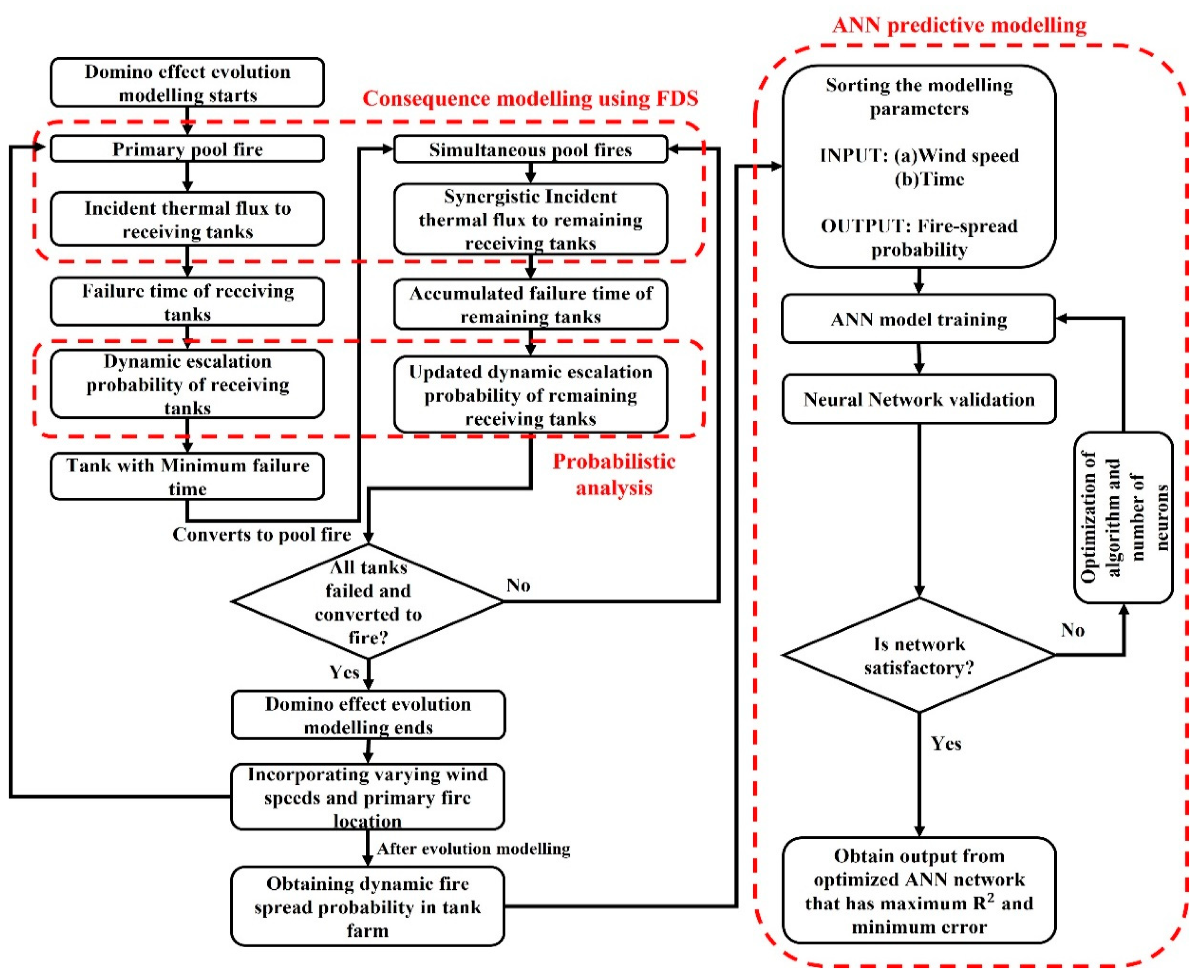
This research assesses the fire-induced domino effect dynamically using FDS. Fire-domino evolution in tank farm is studied under different wind speeds and primary unit placement. Overall dynamic fire spread probability is estimated using individual tank probabilities for each wind speed. The dynamic fire spread probability in tank farms under varying wind conditions could represent the overall meso-level risk. This may allow the emergency response team to revise the intervention timing, so fire spread probability is acceptable at that arrival time given wind conditions. This study uses dynamic probability data from a CFD-based domino effect analysis and ANN to predict the transient fire spread probability at any time during the tank farm failure time which to the authors’ best knowledge, has not been performed by past researchers regarding fire-induced domino effect scenarios. Therefore, the aim is to present a method that integrates accurate numerical data (CFD) with machine learning and to develop a predictive model for fire-induced domino effect escalation probability. This could support fire practitioners in direct estimation of the fire spread probability at a given time interval and wind speed. The application of ANNs for this purpose is one of the first attempts in this respect. ANN probability estimates match actual calculations, proving reliability. CFD is computationally expensive, but ANN predicts probability speedily, despite limited interpretability. This method can be used for emergency response planning, dynamic risk analysis, and fire-induced domino effect control.

2. Methodology

Figure 1 depicts the methodology used in this study to perform the predictive modeling of dynamic escalation probability fire-induced domino effect in tank farm. As illustrated the first phase involves detailed consequence modelling of pool fire accident scenario under varying wind conditions using FDS, CFD software. The incident heat fluxes from primary pool fires and the subsequent synergistic contribution resulting due to continually evolving simultaneous pool fires in the complete domino evolution process is also performed using FDS. Utilizing the incident heat flux data from FDS, the dynamic escalation probabilities of individual tanks and subsequent fire spread probability in complete tank farm is determined through probit-based probabilistic assessment. The comprehensive simulation data is then utilized to develop a reliable predictive model that anticipates the dynamic fire spread probability based on the wind speed and time. The aim is to develop an accurate model based on CFD simulations that can also be utilized by practitioners who have similar probability data from any source and limited computational resources. In this respect, an artificial neural network (ANN) was utilized for model development (training and validation). The optimal model with minimum error and best R² was obtained for predictive analysis of fire-induced domino effect. Further details of each process are sequentially discussed in this section.

2.1. System Requriement for Model Developement

It is known that CFD modelling of fire-induced domino effect is accurate; however, it could be time demanding [29]. CFD simulations of this nature may require around 360 h on a high-performance workstation. Thus, taking this computational cost into account, the FDS-based data is collected to be utilized in ANN modeling for fire spread probability prediction in a tank farm. In contrast to CFD simulation time, developing and running an ANN model for this data requires much lesser time (around 2 h on a regular configuration PC).

2.2. Consequence Modelling Using FDS

In this research, fire dynamics simulator (FDS) CFD software is used. The software solves numerically a form of Navier–Stokes equation appropriate for low speed thermally driven flows with specific emphasis on smoke and heat transfer from fires [42]. Several past research studies have widely used this software to model pool fire, and it is being thoroughly validated against pool fire experiments [43]. In fact, several past studies used FDS and performed extensive validation of pool fire consequences against experiment [44,45,46].

2.3. Dynamic Fire-Induced Domino Effect Evolution Modelling

Pool fire is the credible accident scenario in tank farms. In this study, it is assumed that when a tank fails it loses its integrity completely and converts directly to diked pool fire on the ground. This agrees with past research performed on fire-induced domino effect [28,29,30]. In this study, the primary unit’s pool fire affects nearby tanks due to heat radiation. This promotes a fire-induced domino effect, leading nearby tanks to fail and ignite, intensifying the consequence. FDS version 6.5.3 is used in this research for transient modelling the fire-induced domino effect in tank farm. Wind speed in CFD modelling can affect the fire’s propagation path, causing premature tank failures in the flame tilt direction. The transient thermal radiations from primary pool fire to the surrounding tanks in tank farm are used to obtain the failure time of all the tanks due to primary pool fire are calculated using Equation (1) [47].

$$tt{f}_i=\left\{exp\left[-1.128ln\left(I_i\right)-2.667\times {10}^{-5}{V}_i+9.877\right]/60\right\}i=1, 2, 3,\dots ,n$$

(1)

‘i’ is number of tanks exposed to primary pool fire; ttf_i is failure time (mins) of exposed tanks; I_i is incident heat flux (kW/m²); and V_i is the tanks volume (m³).

The tanks with earliest TTF are considered failing and are converted to pool fire. The CFD modelling is extended where the newly burning tank and previous pool fire burn simultaneously affecting other tanks due to transient accumulated heat flux and the domino effect evolution process continues until the last tank fails. The accumulated time to failure of tanks under the synergistic effect of multiple pool fires is calculated using Equations (2) and (3) [10].

$$t_{i,res,s}={\left(\frac{I_{i, s}}{I_{i, s-1}}\right)}^{-1.13}\left(t_{i,s-1}-t_{minimum failure, s-1}\right)i=1, 2, 3,\dots ,n$$

(2)

$$tt{f}_{i,accumulated,s}=t_{i,res,s}+t_{minimum failure, s-1}$$

(3)

t_i,res,s is residual time (mins) of unit i in current stage S; I_i,s is radiation intensity (kW/m²) received by tank i in current stage S; I_i,s−1 is kW/m² received by the tank i at previous stage S−1; t_i,s−1 is elapsed time of tank i in previous stage S−1; t_{minimum failure,s−1} is minimum time to fail of failed tank in stage S−1; and TTF_{i,accumulated,s} is accumulated TTF of tank i in stage S due to synergistic effect.

The TTF from Equations (1)–(3) can be used to obtain the dynamic escalation probability which is shown in Equation (4) and has time-dependent probit function. The formula for the time-dependent probit function is given in Equation (5) [13].

$$DEP\left(t\right)=0.5\left[1+erf\left(\frac{Y\left(t\right)-5}{\sqrt{2}}\right)\right]$$

(4)

$$Y\left(t\right)=12.54-1.847ln\left(ttf\left(t\right)-t_{elapsed till failure}\right)$$

(5)

Here erf is the error function, and t_{elapsed till failure} is the time elapsed from the start of fire till respective failure.

Using the dynamic escalation probability results, the tanks that most contribute to elevating the escalation probabilities of other tanks could be determined.

2.4. Validation of FDS Pool Fire Model

A kerosene pool fire experiment conducted by Yamaguchi and Wakasa [48] is used to validate the FDS simulation by comparing the incident heat flux. Figure 2 shows the comparison incident heat flux predicted by FDS at distances L/D = 1, 2, 3 from the center of pool fire. As shown in Figure 2, FDS overpredicted the incident heat flux at near distance from pool fire which was also seen in the validation study of Ahmadi et al. [29]. A possible reason for overprediction of incident heat flux at near distance could be that for liquid fuel pools, FDS considers burner surface and does not consider heat release rate losses to the fuel pan, which could be present in the actual experiment and attribute to the incident thermal flux overprediction by FDS at very near distance to the pool fire [49]. However, FDS agrees with experimental heat flux values at farther distances with a 7% deviation, which is within the range of tanks distances of this investigation and is regarded acceptable.

2.5. Dynamic Escalation Probability Verification

The predicted incident heat flux at tanks and resulting dynamic escalation probability from current FDS model is verified against the dynamic escalation probability performed by Ding et al. [50].

In their work, a five-tank case study taken from [10] was considered where the fire-induced domino effect evolution modelling was performed, and dynamic escalation probability was calculated using Ding et al. [50] approach. The tank farm layout along with the separation distance is shown in Figure 3. In the study of Ding et al. [50], ALOHA software was used for the calculation of incident heat flux due to respective pool fires. Current work employed CFD software, to estimate pool fire thermal flux.

Table 1. FDS model input parameters used in the verification.

Input Parameters	Value	Reference
Benzene heat of combustion (kJ/kg)	44,700	[51]
Acetone heat of combustion (kJ/kg)	29,100	[51]
Benzene radiative fraction	0.6	[42]
Acetone radiative fraction	0.27	[42]
Benzene density (kg/m3)	874	[52]
Acetone density (kg/m3)	782	[53]
Benzene mass loss rate per unit area (kg/m2s)	0.048	[54]
Acetone mass loss rate per unit area (kg/m2s)	0.041	[54]
Number of solid angles	500	[29]
Domain size (m)	88 × 70 × 30

lists simulation inputs and Figure 4 shows the mesh independence analysis where the optimal simulation grid size obtained was 0.5 m. The mesh boundaries were open to imitate ambient air conditions, except for ground, which was INERT.

Figure 5 depicts the comparison of the dynamic escalation probabilities of tanks obtained from FDS results against the work of Ding et al. [50]. It is seen that the dynamic escalation probability results and individual tank failure times from FDS model agree with the published results with only 1–2% difference in values.

2.6. Fire Spread Probability in Tank Farm

Once the dynamic escalation probability of individual tanks is obtained using Equations (5) and (6), the dynamic fire spread probability in complete tank farm can be obtained using Equation (7) to represent the overall intensity of fire-induced domino escalation under varying wind speeds. The fire spread probability would be the multiplication of individual escalation probabilities of each tank at a given time instant following the given relationship.

$$P_{fire spread}\left(t_i\right)=DEP{\left(t_i\right)}_1\times DEP{\left(t_i\right)}_2\times \dots$$

(6)

$$P_{fire spread}\left(t_n\right)=DEP{\left(t_n\right)}_1\times DEP{\left(t_n\right)}_2\times \dots$$

(7)

where 1, 2, … are the tanks, t_i is the initial time instant and t_n is the last time instant at failure.

2.7. Dynamic Fire Spread Probability Prediction by ANN

Machine learning is one of the predictive modelling techniques that is being extensively used by several researchers in the field of engineering science [55]. In fact, it has been used in predicting the fire behavior that may support in the risk assessment studies [56,57]. Artificial neural networks (ANNs) are dynamic and data-driven in nature and large volumes of process industry data can be utilized to predict the dynamic fire spread probability for fire-induced domino effect analysis. To treat the data, a predictive and adaptable ANN model with an adequate level of accuracy is required. ANNs are statistical modelling techniques that, when compared to traditional correlations, makes them a powerful and efficient forecasting tool for estimating the attributes of complex non-linear systems [58].

One of the most popular types of ANN is the multilayer feed-forward neural network (MLFNN), which employs a backpropagation learning algorithm [58]. These types of artificial neural networks (ANNs) architectures comprise hidden layer(s) that contain computational nodes known as hidden neurons. These hidden neurons have an activation function to process the inputs. The input data is fed into the input layer to introduce the values of inputs to the network, after which it is transmitted to the hidden layer(s) to be processed. Finally, the last hidden layer passes processed data to the output layer, where the results are acquired. Each neuron in the output and hidden layer(s) is linked to every other neuron in the preceding layer [59].

A feed-forward backpropagation neural network based on the Levenberg–Marquardt (LM) algorithm was trained to forecast fire spread based on exposure time and wind speed. The data points used for model development of each tank case were 121. The data points are provided in Appendix A (

Table A1. Data set of dynamic fire spread probability in tank farm at varying wind speed when primary fire occurred at Tank 1, used for data training in artificial neural network (ANN).

	Input		Output		Input		Output
No.	Time (min)	Wind Speed (m/s)	Fire Spread Probability	No.	Time (min)	Wind Speed (m/s)	Fire Spread Probability
1	0	0	0	62	11.6	2	9.00E-01
2	10	0	2.00E-05	63	11.8	2	9.80E-01
3	10.3	0	5.80E-05	64	12.1	2	1
4	10.4	0	7.70E-05	65	0	4	0
5	10.5	0	1.00E-04	66	7.2	4	5.00E-03
6	10.6	0	1.40E-04	67	7.3	4	6.00E-03
7	10.7	0	1.80E-04	68	7.5	4	1.50E-01
8	10.85	0	2.80E-04	69	7.6	4	1.60E-01
9	10.9	0	3.30E-04	70	7.7	4	1.90E-01
10	11.1	0	6.00E-04	71	7.9	4	2.60E-01
11	11.3	0	1.00E-03	72	8.1	4	3.60E-01
12	11.5	0	2.00E-03	73	8.3	4	5.00E-01
13	11.7	0	3.80E-03	74	8.5	4	6.50E-01
14	11.9	0	7.00E-03	75	8.6	4	7.40E-01
15	12.1	0	1.30E-02	76	8.7	4	8.20E-01
16	12.3	0	2.50E-02	77	8.8	4	9.00E-01
17	12.5	0	4.50E-02	78	9	4	9.80E-01
18	12.7	0	8.00E-02	79	9.1	4	9.90E-01
19	13.1	0	2.00E-01	80	9.3	4	1
20	13.3	0	5.00E-01	81	0	6	0
21	13.5	0	7.00E-01	82	5.2	6	1.00E-05
22	13.7	0	8.20E-01	83	5.5	6	4.30E-05
23	13.9	0	9.00E-01	84	5.8	6	2.00E-04
24	14.1	0	9.90E-01	85	5.9	6	2.70E-04
25	14.3	0	1	86	6	6	4.40E-04
26	0	1	0	87	6.1	6	7.00E-04
27	9.9	1	3.00E-05	88	6.3	6	1.80E-03
28	10.1	1	5.00E-05	89	6.5	6	4.50E-03
29	10.3	1	8.60E-03	90	6.75	6	1.40E-02
30	10.5	1	1.50E-04	91	7.1	6	4.65E-02
31	10.7	1	3.00E-04	92	7.3	6	9.00E-02
32	11	1	7.00E-04	93	7.4	6	1.30E-01
33	11.3	1	1.20E-03	94	7.5	6	1.60E-01
34	11.5	1	3.00E-03	95	7.6	6	2.00E-01
35	11.8	1	8.20E-03	96	7.9	6	3.10E-01
36	12	1	1.50E-02	97	8.8	6	9.00E-01
37	12.3	1	4.00E-02	98	9	6	9.90E-01
38	12.5	1	7.40E-02	99	9.2	6	1
39	12.9	1	2.10E-01	100	0	8	0
40	13.3	1	7.00E-01	101	4.6	8	2.00E-05
41	13.5	1	8.20E-01	102	4.8	8	5.00E-05
42	13.7	1	9.50E-01	103	5	8	1.30E-04
43	13.9	1	9.90E-01	104	5.2	8	3.20E-04
45	0	2	0	105	5.4	8	9.00E-04
46	8.4	2	2.00E-04	106	5.6	8	2.00E-03
47	8.6	2	3.40E-04	107	5.9	8	7.00E-03
48	8.7	2	5.00E-04	108	6.1	8	1.30E-02
49	8.9	2	8.40E-04	109	6.4	8	3.00E-02
50	9	2	1.00E-03	110	6.5	8	4.00E-02
51	9.3	2	2.80E-03	111	6.8	8	6.00E-02
52	9.5	2	5.30E-03	112	7	8	8.20E-02
53	9.7	2	9.80E-03	113	7.25	8	1.20E-01
54	9.8	2	1.30E-02	114	7.4	8	1.60E-01
55	10.1	2	3.20E-02	115	7.6	8	2.20E-01
56	10.3	2	5.30E-02	116	8	8	4.00E-01
57	10.5	2	8.00E-02	117	8.3	8	6.50E-01
58	10.7	2	1.10E-01	118	8.5	8	8.20E-01
59	10.8	2	3.00E-01	119	8.8	8	9.00E-01
60	11	2	4.20E-01	120	9	8	1
61	11.3	2	6.50E-01	121	9.1	8	1

and

Table A2. Data set of dynamic fire spread probability in tank farm at varying wind speed when primary fire occurred at Tank 1, used for data training in artificial neural network (ANN).

	Input		Output		Input		Output
No.	Time (min)	Wind Speed (m/s)	Fire Spread Probability	No.	Time (min)	Wind Speed (m/s)	Fire Spread Probability
1	0	0	0	63	8.4	2	9.90E-01
2	7.1	0	1.00E-05	64	8.5	2	1
3	7.2	0	1.40E-05	65	8.6	2	1
4	7.3	0	2.00E-05	66	0	4	0.00E+00
5	7.6	0	4.00E-05	67	4.25	4	1.10E-04
6	7.8	0	7.00E-05	68	4.4	4	3.00E-04
7	8	0	1.00E-04	69	4.5	4	5.60E-04
8	8.2	0	2.20E-04	70	4.6	4	1.10E-03
9	8.4	0	4.00E-04	71	4.7	4	2.00E-03
10	8.6	0	7.80E-04	72	5	4	1.30E-02
11	8.8	0	1.40E-03	73	5.2	4	3.70E-02
12	9	0	3.00E-03	74	5.4	4	8.90E-02
13	9.2	0	5.00E-03	75	5.6	4	1.78E-01
14	9.4	0	9.00E-03	76	5.7	4	2.40E-01
15	9.6	0	1.80E-02	77	5.9	4	5.00E-01
16	9.8	0	3.50E-02	78	6	4	6.30E-01
17	10	0	7.00E-02	79	6.1	4	7.60E-01
18	10.2	0	1.30E-01	80	6.3	4	9.50E-01
19	10.4	0	2.40E-01	81	6.4	4	1
20	10.6	0	4.25E-01	82	0	6	0.00E+00
21	10.8	0	7.00E-01	83	4.9	6	1.00E-04
22	11	0	9.00E-01	84	5	6	1.50E-04
23	11.2	0	9.90E-01	85	5.2	6	2.70E-04
24	11.3	0	9.90E-01	86	5.4	6	5.00E-04
25	11.4	0	1	87	5.6	6	9.00E-04
26	0	1	0	88	5.8	6	1.68E-03
27	7	1	2.20E-04	89	6	6	3.00E-03
28	7.3	1	5.40E-04	90	6.2	6	6.00E-03
29	7.6	1	1.40E-03	91	6.4	6	1.10E-02
30	7.9	1	3.50E-03	92	6.6	6	2.20E-02
31	8.1	1	6.70E-03	93	6.8	6	4.35E-02
32	8.3	1	1.30E-02	94	7	6	8.40E-02
33	8.5	1	2.50E-02	95	7.2	6	1.60E-01
34	8.7	1	4.85E-02	96	7.4	6	3.00E-01
35	8.9	1	9.30E-02	97	7.6	6	5.00E-01
36	9.1	1	1.80E-01	98	7.8	6	7.60E-01
37	9.2	1	2.40E-01	99	8	6	9.50E-01
38	9.4	1	4.25E-01	100	8.3	6	1
39	9.6	1	6.75E-01	101	0	8	0
40	9.7	1	8.10E-01	102	5.85	8	1.10E-04
41	9.9	1	9.70E-01	103	5.9	8	1.30E-04
42	10	1	9.90E-01	104	6.1	8	2.20E-04
43	10.1	1	9.97E-01	105	6.3	8	4.10E-04
45	10.2	1	1	106	6.5	8	7.40E-04
46	0	2	0.00E+00	107	6.7	8	1.40E-03
47	6	2	8.00E-05	108	6.9	8	2.60E-03
48	6.2	2	2.30E-04	109	7	8	3.50E-03
49	6.3	2	3.40E-04	110	7.2	8	6.70E-03
50	6.5	2	7.70E-04	111	7.4	8	1.30E-02
51	6.7	2	1.44E-03	112	7.6	8	2.50E-02
52	6.9	2	2.40E-02	113	7.8	8	4.85E-02
53	7	2	3.30E-02	114	8	8	9.40E-02
54	7.2	2	6.40E-02	115	8.2	8	1.80E-01
55	7.4	2	1.20E-01	116	8.3	8	2.40E-01
56	7.5	2	1.70E-01	117	8.5	8	4.25E-01
57	7.6	2	2.30E-01	118	8.7	8	6.75E-01
58	7.8	2	4.00E-01	119	8.8	8	8.20E-01
59	7.9	2	5.20E-01	120	9	8	9.70E-01
60	8	2	6.50E-01	121	9.2	8	1
61	8.2	2	8.90E-01	122	9.3	8	1
62	8.3	2	9.60E-01

). FDS-based fire spread probability data was divided into three groups for ANN modelling: training (70%), validation (15%), and testing (15%). The number of hidden layers, hidden layer neurons, activation functions, and learning method were modified. The neural network lowers estimated response error using backpropagation. Levenberg–Marquardt neural network has a faster training process and was chosen. The Levenberg–Marquardt algorithm uses Gauss–Newton and gradient descent [60]. The gradient descent approach reduces the sum of quadrated errors by updating the steepest downward direction parameters [61].

Gauss–Newton reduces total squared error by assuming the parameter’s least square function is locally quadratic and assessing its minimum value. Levenberg–Marquardt operates as a gradient-descent when parameters are far from ideal [62]. The Gauss–Newton approach, on the other hand, works best when the parameters are near their optimum values [61]. Figure 6 illustrates the neural network’s architecture to obtain the fire spread probability based on wind speed and time. There are two nodes in the input layer, sixteen in the hidden layer, and one node in the output layer.

The sigmoid function, denoted by Equation (8) [63], was employed in the hidden layer neurons. However, the output layer processed data using a linear function known as ‘purelin.’ The hidden layer’s activation function transforms the input data into a form that the output layer can recognize.

$$f\left(x\right)=\frac{e^x-e^{-x}}{e^x+e^{-x}}$$

(8)

$$x_j={{\displaystyle \sum }}_{i=1}^N{w}_{ij}{y}_i+b_j$$

(9)

where x in Equation (8) is the weighted sum of the inputs, which is calculated in terms of weights (w), biases (b), and output (y) according to Equation (9) [59,64].

2.8. Performance Evaluation Indices for ANN

The following performance indices are used to determine the accuracy of ANN and to determine if the predictive model is well suited for predicting dynamic fire-induced domino effect.

Root mean square error (RMSE): It provides information of the overall credibility of the predicted data against actual values in entire data spectrum. The formula to calculate this index is shown in Equation (10) [65].

$$RMSE=\sqrt{\frac{{{\displaystyle \sum }}_{i=1}^N{\left({\mathit{Prob}}_i^{calculated}-{\mathit{Prob}}_i^{\mathit{Pred}}\right)}^2}{N}}$$

(10)

Mean absolute error (MAE) is a scale-dependent accuracy measurement index which averages the absolute error in the data set. This index measures unbiased variation in data set equally. This index is best suited to obtain the errors for time-based data analysis. The formulae to calculate MAE is given in Equation (11) [65].

$$MAE=\frac{1}{N}{\displaystyle \sum }_{i=1}^N\left|{\mathit{Prob}}_i^{calculated}-{\mathit{Prob}}_i^{\mathit{Pred}}\right|$$

(11)

Mean relative error (MRE): Calculates the relative statistical error in predicted data set specially for lower magnitude of data set such as the fire spread probability in this case and the expression is shown in Equation (12) [65].

$$MRE=\frac{1}{N}{\displaystyle \sum }_{i=1}^N\left(\frac{{\mathit{Prob}}_i^{calculated}-{\mathit{Prob}}_i^{\mathit{Pred}}}{{\mathit{Prob}}_i^{calculated}}\right)$$

(12)

R² is the coefficient of determination that describes the proportion of the total statistical variance for the observed dependent variable (probability of fire spread) data set that can be explained the input variables (wind speed and time) in the model (Equation (13)) [65].

$$R^2={\left(\frac{{{\displaystyle \sum }}_{i-1}^N\left({\mathit{Prob}}_i^{\mathit{Pred}}-{\mathit{Prob}}_i^{\mathit{calculated}}\right)\left({\mathit{Prob}}_i^{\mathit{Pred}}-{\mathit{Prob}}_i^{\mathit{calculated}}\right)}{\sqrt{{{\displaystyle \sum }}_{i=1}^N{\left({\mathit{Prob}}_i^{\mathit{calculated}}-{\mathit{Prob}}_i^{\mathit{CalcMean}}\right)}^2{{\displaystyle \sum }}_{i=1}^N{\left({\mathit{Prob}}_i^{\mathit{Pred}}-{\mathit{Prob}}_i^{\mathit{PredMean}}\right)}^2}}\right)}^2$$

(13)

2.9. Modelled Tank Farm

The proposed methodology is implemented on a case study taken from Zhou et al. [66] shown in Figure 7. The study uses an oil depot of 6 equal-sized gasoline atmospheric storage tanks with diameter of 20 m, and their heights are 10 m. The separation distance between tanks is 30 m as shown in Figure 7 and the credible accident scenario for all tanks is pool fire. The tank spacing meets NFPA 30 requirement [67]. Two primary accident scenarios include the following: (a) Primary fire at Tank 1(b) Primary fire at Tank 4 are chosen for the domino propagation analysis. The respective wind direction is also shown in Figure 7. The wind speeds considered in this study are 0 m/s, 0.5 m/s, 1 m/s, 2 m/s, 4 m/s, 6 m/s, and 8 m/s, which lie in the range of frequently occurring wind speeds in Malaysia [68]. The pool fire is modelled at ground level. The input parameters required to model pool fire in tank farm using FDS are given in

Table 2. FDS input parameters used to model pool fire in tank farm.

Input Parameters	Value	Reference
Fuel	gasoline	[66]
Pool diameter (m)	20
Fuel heat of combustion (kJ/kg)	44,100	[51]
Soot yield (kg/kg)	0.038	[70]
Radiative fraction	0.4	[42,70]
Fuel density (kg/m3)	715	[71]
Fuel mass loss rate per unit area (kg/m2s)	0.055	[69]
Steel density (kg/m3)	7850
Steel Specific heat (kJ/kg.K)	0.46
Steel Conductivity (W/m.K)	45.8
Steel emissivity	0.7
Steel Absorption coefficient (1/m)	0.0005
Number of solid angles	500	[29]
Domain size	120 × 90 × 55

.

Figure 8 shows the tank farm CFD model. The simulation domain is 100 m × 70 m × 55 m. The mesh boundaries were maintained open to reflect open boundary circumstances. The LES turbulence model was utilized to model large domain fluid flow interactions [31]. The pool fire is modelled on ground as a fixed source and constant mass loss rate per unit area (MLRPUA) is applied which also complies the past CFD research by Ahmadi et al. [29] on domino effect. The MLRPUA of gasoline used in this research is calculated using Zabetakis–Burgess method, which is considered suitable by past researchers and is also used in their pool fire domino effect investigation [30,69]. The tank material used in this setup is ‘steel’ and all the properties are imported from the FDS material property library in the software. The default material properties defined in the code are also provided in Table 2. The given values were also being used by the FDS developers in their validations.

3. Results and Discussions

CFD modelling of fire spread between storage tanks in domino evolution process is a complex task which could involve numerous influencing parameters. Furthermore, in FDS, and unlike other commercial CFD software packages, the more output quantities provided in the input code, the more simulation time is demanded and greater is the storage space requirement. Nevertheless, most of the past CFD-based research on fire-induced domino effect took into consideration only the incident heat flux in their analysis.

Therefore, in this study, radiative heat flux devices were placed at each tank to monitor the incident heat flux values at different tank wall locations along with slice files of incident thermal flux under varying wind speeds. Recent study by Li et al. [31] analyzed the detailed distribution of incident heat flux on atmospheric storage tanks by placing large number of radiative heat flux devices on the respective tanks exposed to pool fire. Under low wind speeds, the top of a tank exposed to a pool fire receives the most thermal flux, whereas under stronger winds, the mid-to-lower region does. Similar conclusions were also obtained in the previous study of Ahmadi et al. [29]. Therefore, it can be deduced from the comprehensive work of Li et al. [31] that key differences in the heat flux values were at the top, middle, and bottom of the tank (such as the proposed location in this research).

In fire-induced domino effect, the accident evolves by promoting progressive multiple pool fires and the incident heat flux changes due to synergistic effect. In present research, during the successive domino evolution process, the maximum value of incident heat flux out of all devices for each tank and is used for further escalation probability calculation to represent worst case scenario, such as what was considered by Li et al. [31].

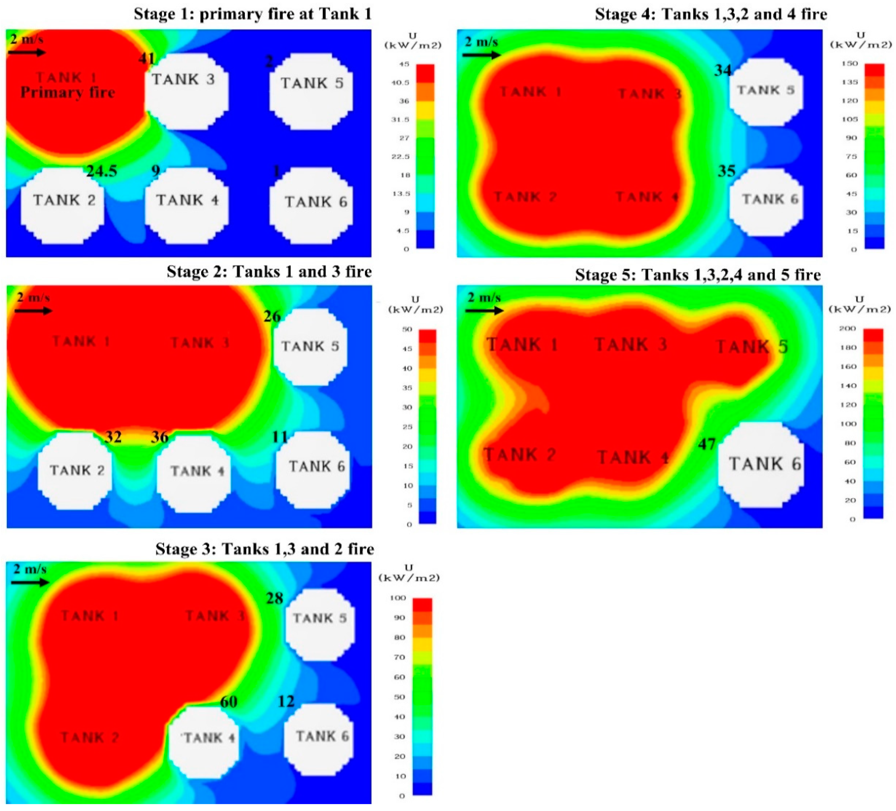
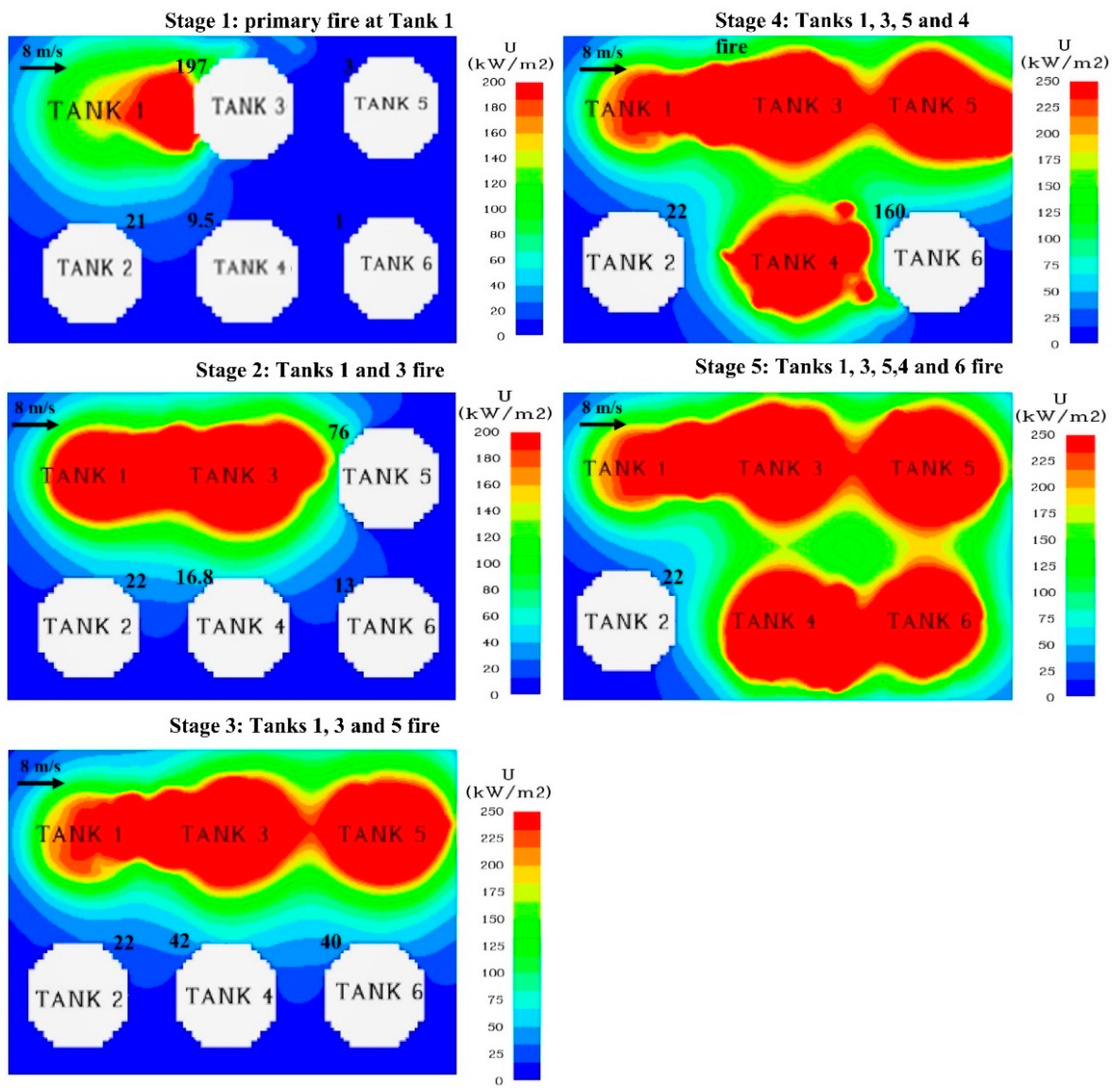
Figure 9 and Figure 10 illustratively show the spatial contours of heat flux distribution in the complete domino evolution due to primary fire at Tank 1, under 2 m/s and 8 m/s wind speeds, respectively. Figure 9 shows that at 2 m/s wind speed, inline Tanks 3 and 5 receive more heat than offset tanks. Tank 3, downwind from the primary pool fire, receives the most thermal flux. Tank 2 transforms to fire in stage 3 when Tank 3 fails owing to its proximity to the primary fire. The fire at primary Tank 1 and inline Tank 2 enhanced Tank 4’s vulnerability by more than five times compared to merely the primary fire, generating a domino effect at stage 4.

Figure 10 shows that when wind speed reached 8 m/s, inline tanks became further vulnerable due to significant incident thermal flux. At stage 2, distant Tank 5 obtained 25 times more heat flux compared to when influenced by Tank 1 fire. Tank 2 was not harmed by high wind domino evolution.

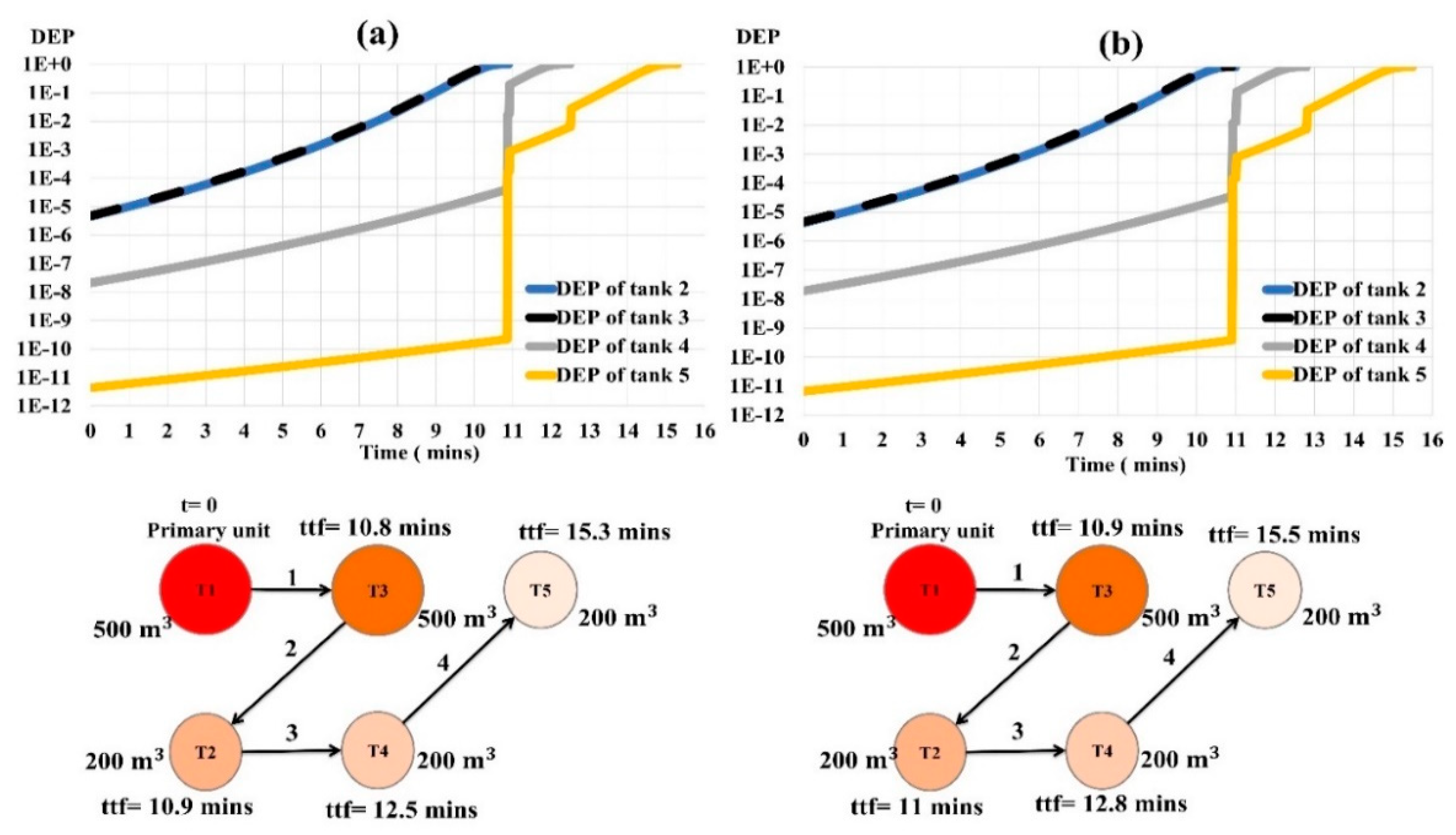
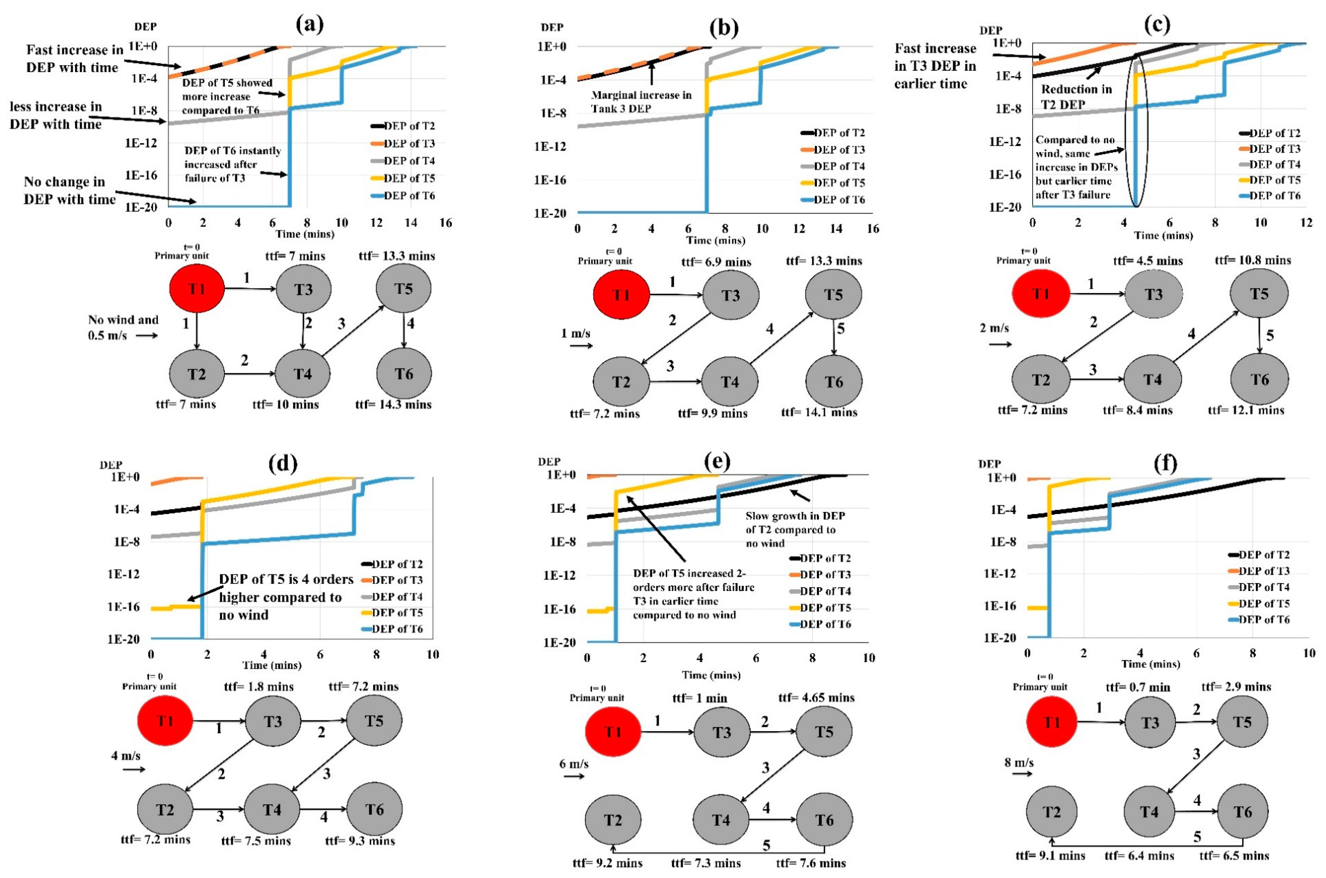
The dynamic escalation probabilities (DEP) of individual tanks due to incident thermal flux and resulting escalation path during the domino evolution process under varying wind speeds, when the primary fire occurred at Tank 1, are shown in Figure 11.

Table 3. The Maximum incident heat flux at tanks in the domino evolution process under varying wind speeds when the primary fire occurred at Tank 1.

Maximum Incident Heat Flux (kW/m2) on Respective Tanks under Varying Winds
Primary Fire at Tank 1
0 m/s and 0.5 m/s								4 m/s
Progressive tanks on fire 1	Heat receiving tanks 2	T1	T2	T3	T4	T5	T6	Progressive tanks on fire 1	Heat receiving tanks 2	T1	T2	T3	T4	T5	T6
T1 fire		-	27.5	27.5	8	1.2	1	T1 fire		-	23	92	12	3	1.4
T1 T3 T2 fire		-	-	-	45	26	11	T1 T3 fire		-	28	-	23	34	10
T1 T3 T2 T4 fire		-	-	-	-	33	33	T1 T3 T2 T5 fire		-	-	-	132	-	35
T1 T3 T2 T4 T5 fire		-	-	-	-	-	45	T1 T3 T2 T5 T4 fire		-	-	-	-	-	66
1 m/s								6 m/s
Progressive tanks on fire 1	Heat receiving tanks 2	T1	T2	T3	T4	T5	T6	Progressive tanks on fire 1	Heat receiving tanks 2	T1	T2	T3	T4	T5	T6
T1 fire		-	27.5	28	8	1.2	1	T1 fire		-	21	154	10	3	1.3
T1 T3 fire		-	38	-	39	25	10	T1 T3 fire		-	22	-	17	49	13
T1 T3 T2 fire		-	-	-	47	26	11.5	T1 T3 T5 fire		-	22	-	44	-	40
T1 T3 T2 T4 fire		-	-	-	-	33	34	T1 T3 T5 T4 fire		-	22	-	-	-	86
T1 T3 T2 T4 T5 fire		-	-	-	-	-	45	T1 T3 T5 T4 T6 fire		-	22	-	-	-	-
2 m/s								8 m/s
Progressive tanks on fire 1	Heat receiving tanks 2	T1	T2	T3	T4	T5	T6	Progressive tanks on fire 1	Heat receiving tanks 2	T1	T2	T3	T4	T5	T6
T1 fire		-	24.5	41	9	2	1.3	T1 fire		-	21	197	9.5	3	1
T1 T3 fire		-	32	-	36	26	11	T1 T3 fire		-	22	-	16.8	76	13
T1 T3 T2 fire		-	-	-	60	28	12	T1 T3 T5 fire		-	22	-	45	-	42
T1 T3 T2 T4 fire		-	-	-	-	34	35	T1 T3 T5 T4 fire		-	22	-	-	-	160
T1 T3 T2 T4 T5 fire		-	-	-	-	-	47	T1 T3 T5 T4 T6 fire		-	22	-	-	-	-

¹ Progressive tanks on fire are represented column-wise. ² Heat receiving tanks are represented row-wise.

lists the maximum received thermal fluxes by tanks in the complete domino evolution process under all considered wind speeds.

Figure 11a shows that the tanks’ dynamic escalation probability and path are same under no wind and 0.5 m/s wind. Tanks 2 and 3 adjacent to primary fire show faster dynamic escalation probability development, followed by Tank 4. Tanks 5 and 6 show no change until 7 min. 0.5 m/s winds did not affect escalation dynamics. Figure 11b shows that when the wind speed increased to 1 m/s, Tank 3’s DEP increased slightly with only a 1% reduction in failure time. Tank 3’s dynamic escalation probability increased by an order under 2 m/s wind, forcing it to fail 37% earlier than without wind. Due to Tank 3’s earlier failure, all other tanks collapsed earlier with increasing wind speed compared to no wind. Inline tanks are more vulnerable to high winds than offset tanks. Under 2 m/s wind speed, Tank 5’s failure time decreased by 19%, while offset Tanks 4 and 6 decreased by 16%. Tank 2’s offset location slows its dynamic escalation.

Wind speeds of 4 m/s changed the dynamics of the tank farm’s fire-induced domino effect. Windspeed enhanced the inline tanks’ susceptibility. Tanks 3 and 5 fail 74% and 46% faster under 4 m/s wind than in no wind. Tank 3’s dynamic escalation probability increased by 2 orders from the initial time and reached 1 at 1.8 min; under windless conditions, it was 1 × 10⁻⁴. Tank 5’s initial escalation probability was 1 × 10⁻²⁰, but 4 m/s wind raised it to 1 × 10⁻¹⁶. When the wind speed increased to 6 m/s and 8 m/s, Tank 3 and Tank 5 failed earlier due to dynamic escalation. Figure 10f and Figure 11e show that for 6 m/s and 8 m/s wind speeds, Tank 3’s escalation probability neared 1 very quickly, whereas Tank 5’s elevated from 1 × 10⁻¹⁶ to 8 × 10⁻² in around 1 min.

Hence, in addition to the obvious increase in Tank 3 vulnerability due to primary fire flame under wind speed, Tank 5 probability of failure progressively increased in the domino evolution as wind speed increased. Only Tank 2’s susceptibility and failure time decreased among the offset tanks. Figure 11e,f show that the failure of other tanks in the tank farm does not increase Tank 2’s dynamic escalation likelihood. It is also deduced that the increase in wind speed kept changing the propagation path of domino effect. The complete tank farm failed before the active intervention time of 15 min [72] even under no wind condition.

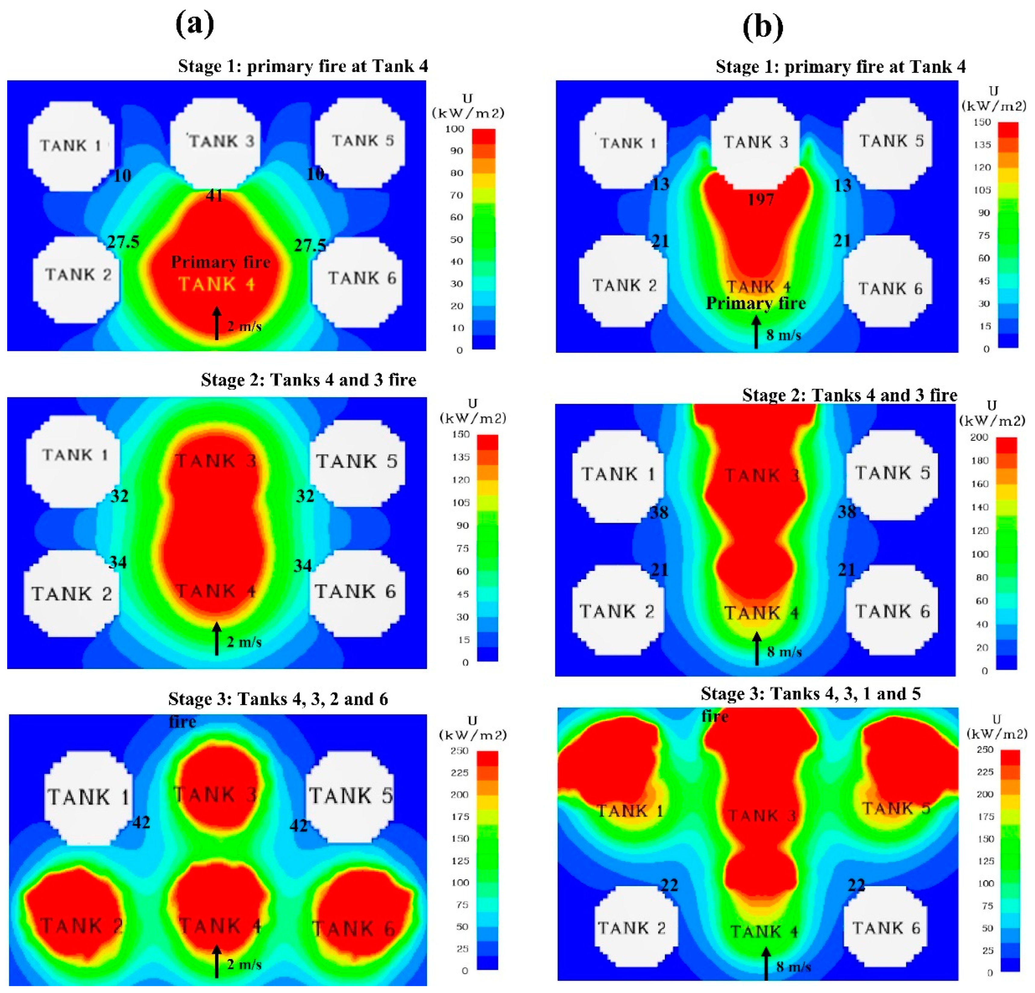
Figure 12 shows how incident thermal flux on nearby tanks was observed after Tank 4 caught fire and during the successive fire escalation. With 8 m/s winds pushing down the flame, tanks receive maximum heat flux in the center. Tank 3 was most vulnerable since it was immediately in front of the primary pool fire and received the most heat at all wind speeds.

Table 4. The maximum incident heat flux at tanks in the domino evolution process under varying wind speeds when the primary fire occurred at Tank 4.

Maximum Incident Heat Flux (kW/m2) on Respective Tanks under Varying Winds
Primary Fire at Tank 4
0 m/s and 0.5 m/s								4 m/s
Progressive tanks on fire 1	Heat receiving tanks 2	T1	T2	T3	T4	T5	T6	Progressive tanks on fire 1	Heat receiving tanks 2	T1	T2	T3	T4	T5	T6
T4 fire		8	27.5	27.5	-	8	27.5	T4 fire		9.5	23	92	-	9.5	23
T4 T3 T2 and T6 fire		32.5	-	-	-	32.5	-	T4 T3 fire		42	30	-	-	42	30
								T4 T3 T1 and T5 fire		-	32	-	-	-	32
1 m/s								6 m/s
Progressive tanks on fire 1	Heat receiving tanks 2	T1	T2	T3	T4	T5	T6	Progressive tanks on fire 1	Heat receiving tanks 2	T1	T2	T3	T4	T5	T6
T4 fire		8	27.5	28	-	8	27.5	T4 fire		9.5	23	154	-	9.5	23
T1 T3 fire		32	34	-	-	32	34	T4 T3 fire		46	23	-	-	46	23
T1 T3 T2 and T6 fire		41	-	-	47	41	11.5	T4 T3 T1 and T5 fire		-	25	-	-	-	25
2 m/s								8 m/s
Progressive tanks on fire 1	Heat receiving tanks 2	T1	T2	T3	T4	T5	T6	Progressive tanks on fire 1	Heat receiving tanks 2	T1	T2	T3	T4	T5	T6
T4 fire		9	24.5	41	-	9	24.5	T4 fire		9.5	21	197	-	9.5	21
T4 T3 fire		32	34	-	-	32	34	T4 T3 fire		38	21	-	-	38	21
T4 T3 T2 and T6 fire		42	-	-	-	42	-	T4 T3 T1 and T5 fire		-	22	-	-	-	22

¹ Progressive tanks on fire are represented column-wise. ² Heat receiving tanks are represented row-wise.

lists the maximum incident heat flux in complete domino progression for calculating failure time and dynamic escalation likelihood.

Figure 13 shows tank failure times and dynamic escalation probability under different wind speeds when Tank 4 was on fire. Dynamic evolution modelling and computations show that escalation under primary fire at Tank 4 with varying wind conditions is very different. In such a situation, circumstances may worsen because the major fire is in the tank farm and impacts nearby tanks. According to dynamic escalation estimations, when wind speeds increase, Tank 3’s failure decreases, while Tanks 2 and 6’s susceptibility grows up to 4 m/s and then drops due to flame effect at Tank 4’s primary fire. Downwind enhances a tank’s vulnerability. Figure 13a shows that Tank 5’s dynamic escalation probability rises from 6 × 10⁻⁹ to 3 × 10⁻³ in 7 min owing to primary fire at Tank 4 and no wind. Tank 5 failed in the third stage when its dynamic escalation probability went from 1 × 10⁻²⁰ to 1 × 10⁻⁴ in 7 min at the second stage and subsequently to 1 × 10⁻² in 10 min at the third level (Figure 11a). Figure 13a shows how the mid-located initial fire at Tank 4 produced simultaneous failures at Tanks 2, 3, and 6 with the same dynamic escalation. Under no wind, the entire tank farm collapses 21% earlier when Tank 4 is on fire compared to Tank 1 under the same conditions (Figure 11a and Figure 13a).

Figure 13c shows that at 2 m/s, Tank 3 failed at 4.5 min due to the flame influence of Tank 4’s primary fire. Tank 3’s failure dynamically raises all tanks’ escalation risk. The escalation probability growth rate did not alter when the wind speed was 2 m/s compared to windless conditions. Due to lower starting escalation probabilities, Tanks 1 and 5 fail after 8.6 min. Tank 5’s dynamic escalation probability increased from 1 × 10⁻⁹ to 1 × 10⁻³ after 4.5 min under primary fire at Tank 4, while it increased less from 1 × 10⁻²⁰ to 1 × 10⁻⁸ under 2 m/s wind speed. At 2 m/s, tank farm failure time is reduced by 25% compared to no wind.

Figure 13 shows how the fire spread dynamics change after Tank 3 fails under 4 m/s. The dynamic escalation probability profile shows that Tanks 1 and 5 have an escalation probability of 1 × 10⁻⁷ before Tank 3 failure which jumped to 1 × 10⁻² after Tank 3 fails at 1.8 min. At 4 m/s wind speed, Tanks 1 and 5 have a higher dynamic escalation probability than at 2 m/s. At this wind speed, the tank farm collapses 44% sooner than without wind. As the wind speed increased to 6 m/s and 8 m/s, downwind tanks experienced early failure and a large dynamic increase in escalation probability (Figure 13e,f). More tanks are in the offset direction of wind and flame’s propagation direction, hence as wind speed increases, the tank farm’s failure time delays.

3.1. Tank Farm Dynamic Fire Spread Probability

Figure 14 shows the dynamic fire spread probability due to fire-induced domino effect in the tank farm under varying wind speed.

The tank farm dynamic fire spread probability is based on the dynamic escalation probabilities of individual tanks. Figure 14a illustrates the dynamic evolution of fire escalation probability when the primary fire occurred in Tank 1, and Figure 14b shows fire spread probability when the fire occurred in Tank 4, in the middle of the tank farm.

When Tank 1 caught fire, and under 0 m/s and 1 m/s winds, fire spread probability is similar. At 2 m/s, tank farm vulnerability to domino effect increased, leading fire spread probability to rise earlier than at lower wind speeds. This trend remained as wind speed increased, but dynamic fire spread probabilities were near after 4 m/s. After 4 m/s, the tank farm in the primary fire at Tank 1 showed minimal reduction in total tank farm failure (Figure 11). Figure 14a shows a decrease in dynamic fire spread probabilities at 4 m/s and above.

Figure 14b shows how the dynamic fire spread probability changed when the primary fire was at Tank 4, in the middle of the tank farm. The dynamic fire spread probability grew earlier as wind speed increased from 0 to 4 m/s; however, after this wind speed, tank farm vulnerability was less influenced, and the probability increased later.

Figure 14 shows that for all wind speeds, the dynamic fire spread probability is low at first and eventually rises to unity. The domino escalation probability threshold is 10⁻⁵ [73]. This dynamic probability analysis estimates when the fire spread probability reaches the escalation probability threshold. Figure 14a shows that a primary fire at Tank 1 in windless conditions reached the threshold in 10 min. This fire spread probability threshold was met 58% early at 8 m/s. This reveals that wind contributes significantly to dynamic fire escalation, so emergency response teams should plan for it. When Tank 4 was on fire, the escalation probability threshold was achieved earlier due to simultaneous pool fires.

3.2. Probabilistic Determination of Most Vulnerable Tank

Figure 15 shows time-dependent escalation probability under varied winds for each tank. The dynamic escalation probability of tanks identifies the tanks that produce the most dynamic escalation. Figure 15a–c show that when Tank 1 caught fire, Tank 3 was the most contributing tank since its failure increased the escalation probabilities of other tanks at all wind speeds. Tank 3 is in the middle of a tank farm; therefore, its fire affects other tanks around it since Tank 1 is on fire. Tank 3’s fire raised the escalation probability of all tanks at all wind speeds, but most for downwind Tanks 5 and 6. Tank 2 has the highest initial dynamic escalation probability (between 1 × 10⁻⁵ and 1 × 10⁻⁴) after Tank 3 when the primary fire was at Tank 1, at all wind speeds. This may be owing to Tank 1’s closeness and primary fire. Tank 2 might produce a domino effect with Tank 3. Based on the dynamic escalation probability study, Tanks 2 and 3 are the most susceptible to domino effect.

Figure 16 shows that Tank 3, under fire from Tank 4, raised the escalation probability of adjacent tanks. Figure 16 shows that in the situation of a primary fire at Tank 4.

Hence from the CFD-based dynamic escalation analysis, it was found that the most dangerous tanks in the tank farm were those that surrounded the principal fire (Tanks 2 and 3 when primary fire is at Tank 1, Tanks 2, 3 and 6 when primary fire is at Tank 4). Dynamic escalation probability study in complete domino development shows time-dependent tank farm vulnerability. Using CFD modelling, which accurately models fire’s transient behavior under different wind conditions, and integrating it with dynamic failure probability analysis, the results revealed the modeling’s ability to detect escalation behavior over time, allowing earlier mitigation to prevent complete failure.

3.3. Application and Selection of Best Optimized ANN Model

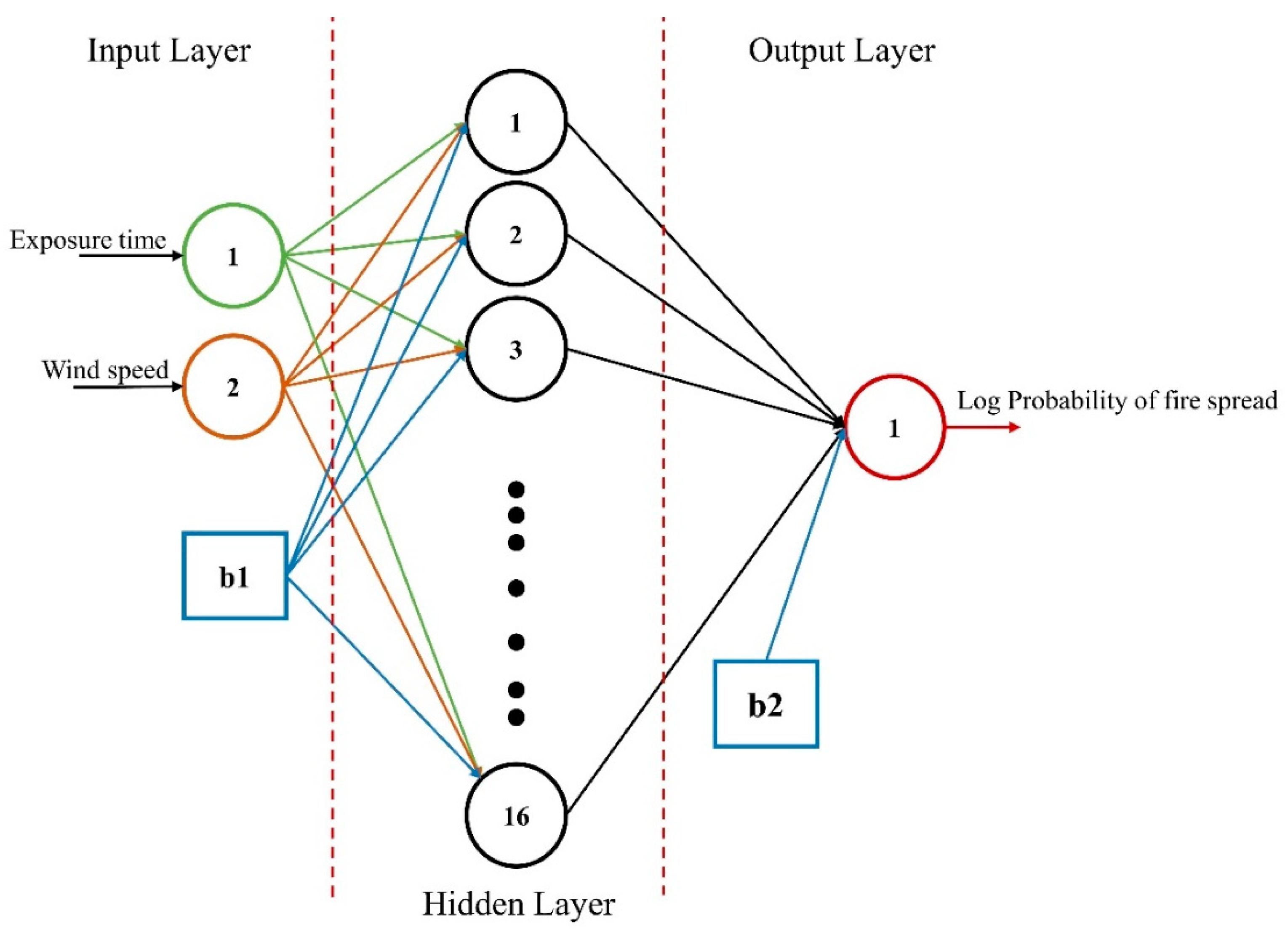
This study uses ANN to optimize a model that can predict dynamic fire spread probability at different times and wind speeds. Since the probability of fire spread is negligibly low at the start, the dynamic fire spread probability data is filtered so that only values above 10⁻⁵ [73] are used. As mentioned earlier, the reader can view the full training data set in Appendix A.

The selection of an appropriately optimized neural network model is critical to the accuracy of future forecasts as well as the practicability of the model that has been trained. In this case, MATLAB 2020b was used to train a feed-forward backpropagation network. Computational values of exposure times and wind speed were provided into the input layer, and simulated log probabilities of fire spread were designated as the desired output, as part of the model’s training phase. After that, the network was trained with a variety of activation functions, and the Levenberg–Marquardt algorithm was determined to be the most suitable with tansigmoid and purelin as activation functions. Various numbers of hidden layers and hidden neurons have been tested to obtain an adequately optimized model. The training data set was utilized to train the network throughout the development of the model, followed by validation to guarantee the network’s high generalization ability. The network was then tested using the testing data set. The performance criterion used was the difference between the actual and expected outputs of the neural network.

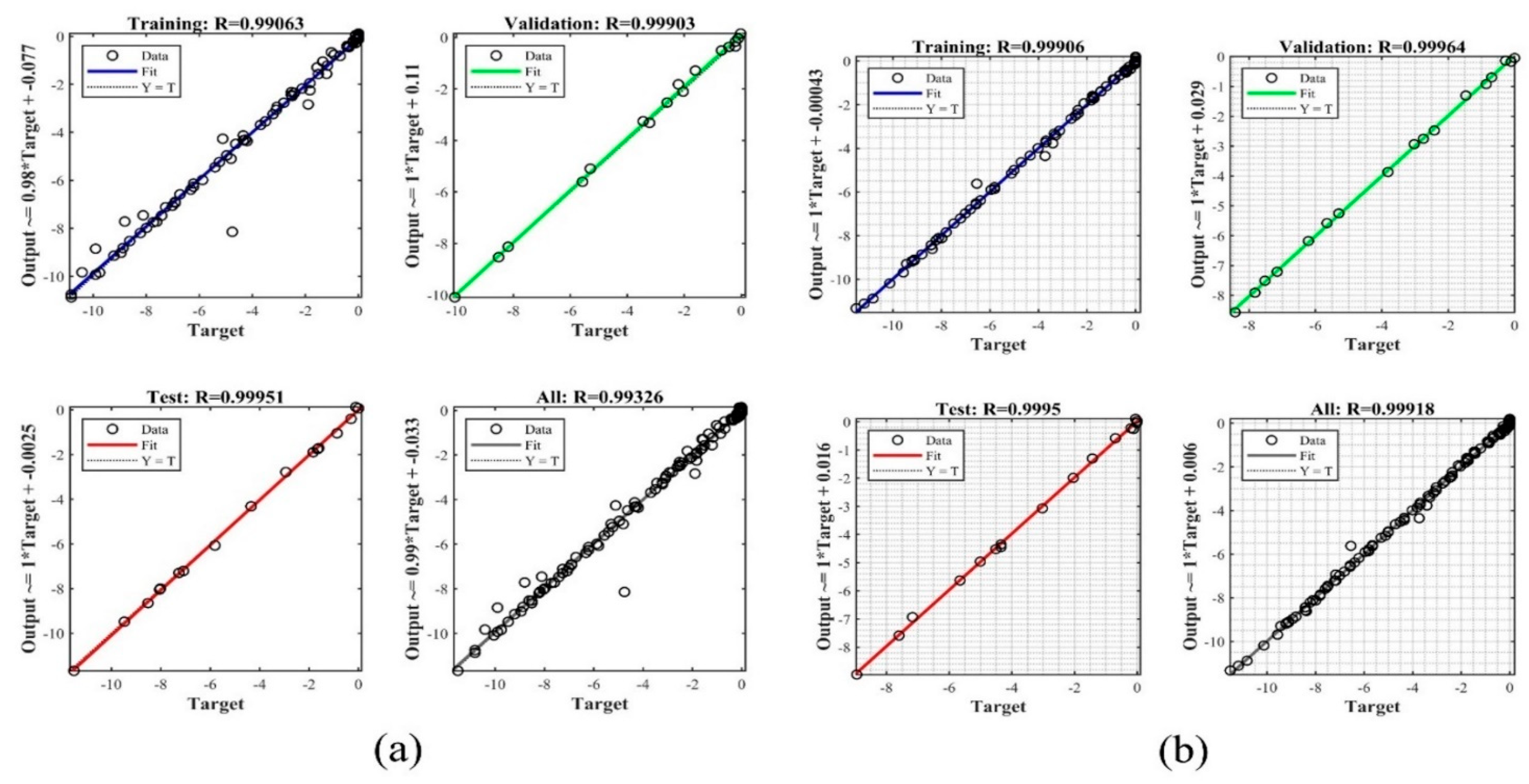
For the most optimized network,

Table 5. MSE and R-squared values for trained models for Tank 1.

Neurons	MSE			R2
	Training	Validation	Testing	Training	Validation	Testing
6	0.25	0.16	0.21	0.976	0.990	0.985
7	0.16	1.14	0.12	0.986	0.916	0.988
8	0.05	0.06	1.51	0.995	0.995	0.906
9	0.22	0.62	0.49	0.979	0.964	0.957
10	0.09	0.15	1.48	0.991	0.987	0.915
12	0.29	1.28	0.59	0.975	0.867	0.964
14	0.16	0.05	1.48	0.987	0.995	0.842
16 1	0.21	0.02	0.016	0.981	0.998	0.999
17	0.90	0.23	0.54	0.941	0.986	0.966

¹ The ANN model (for Tank 1 scenario) with optimized number of hidden layer neurons.

and

Table 6. MSE and R-squared values for trained models for Tank 4.

Neurons	MSE			R2
	Training	Validation	Testing	Training	Validation	Testing
6	0.01	0.02	0.18	0.998	0.998	0.989
7	0.07	0.06	0.14	0.993	0.995	0.985
8	0.006	0.01	0.13	0.999	0.999	0.991
9	0.04	0.15	0.32	0.996	0.984	0.983
10	0.02	0.03	0.05	0.998	0.996	0.992
12	0.01	0.27	0.10	0.999	0.977	0.990
14	0.02	0.02	0.22	0.998	0.996	0.986
16 1	0.02	0.006	0.008	0.998	0.999	0.999
17	0.04	0.07	0.06	0.996	0.990	0.995

¹ The ANN model (for Tank 4 scenario) with optimized number of hidden layer neurons.

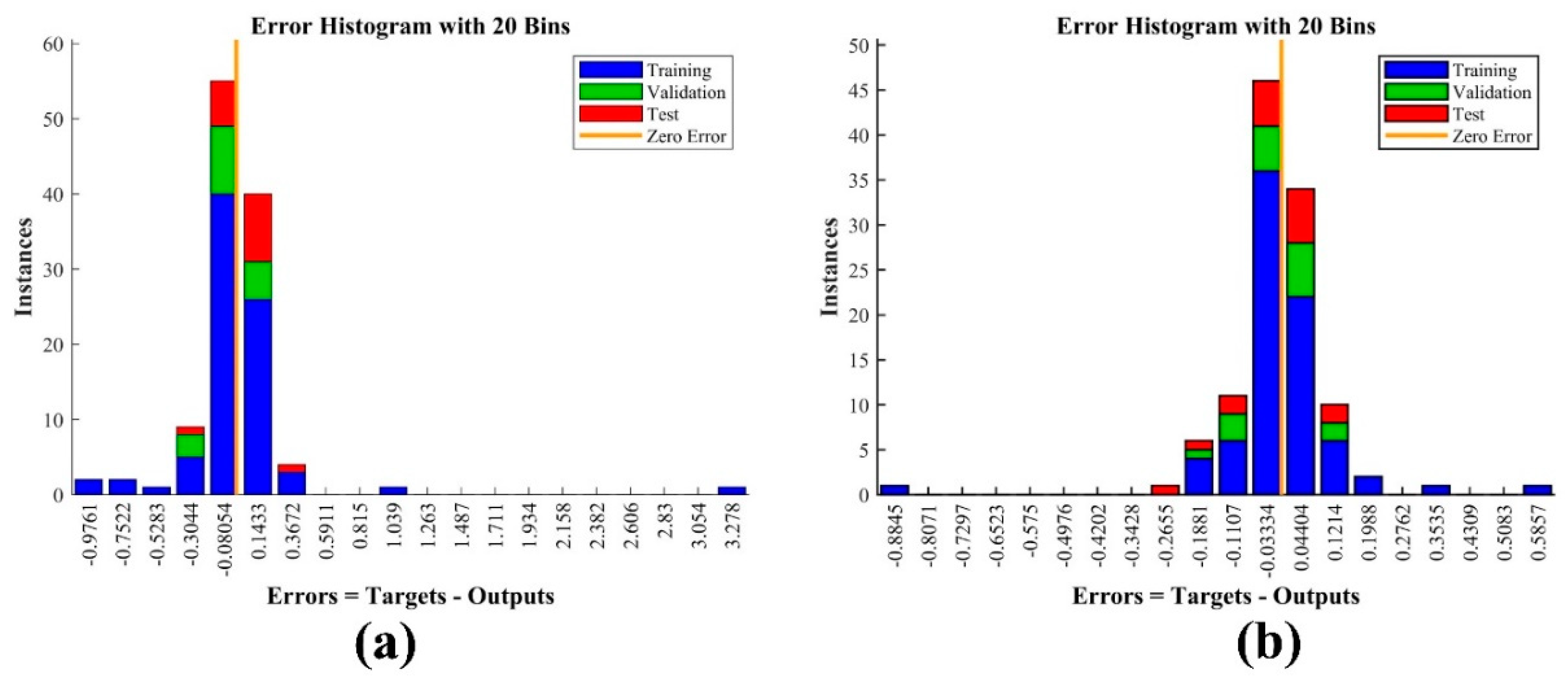
show the MSE (0.21, 0.02, 0.016), R² (0.981, 0.998, 0.999), and MSE (0.02, 0.006, 0.008), R² (0.998, 0.999, 0.999) values for the network’s training, validation, and testing phases, respectively, for Tank 1 and Tank 4. The R values for all the phases and the overall value are also given in Figure 17 along with the error histograms for the trained networks in Figure 18. Such a high R values in ANN model training have also been observed in past research, even for predictions in safety-critical domain [74]. Thus, current trained predictions are precise and accurate based on coefficient regression value.

3.4. Performance Comparison of ANN

The trained models have been tested using different established performance indices such as root mean squared error (RMSE), mean absolute error (MAE), mean relative error (MRE), and coefficient of determination (R-squared). Artificial neural network (ANN) showed robustness in the modelling with significantly high accuracy.

Table 7. Performance indices of ANN for Tank 1 and Tank 4.

	Tank 1				Tank 4
Performance index	RMSE	MAE	MRE	R2	RMSE	MAE	MRE	R2
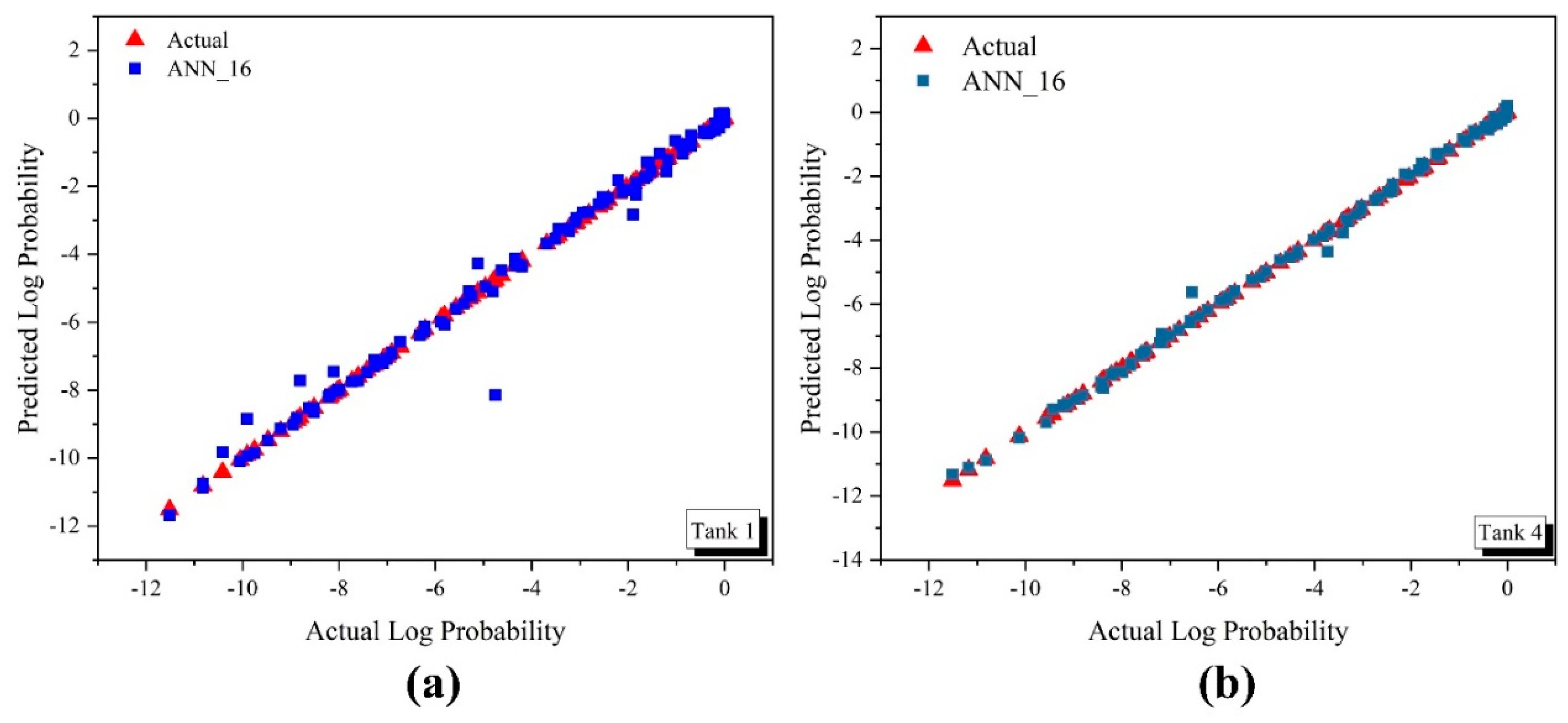
ANN	0.04	0.02	0.14	0.99	0.03	0.01	0.09	0.99

shows the statistical performance indices for ANN modelling approaches. Moreover, the plots of predicted vs. actual fire spread log probabilities are shown in Figure 19 to show the data fitting.

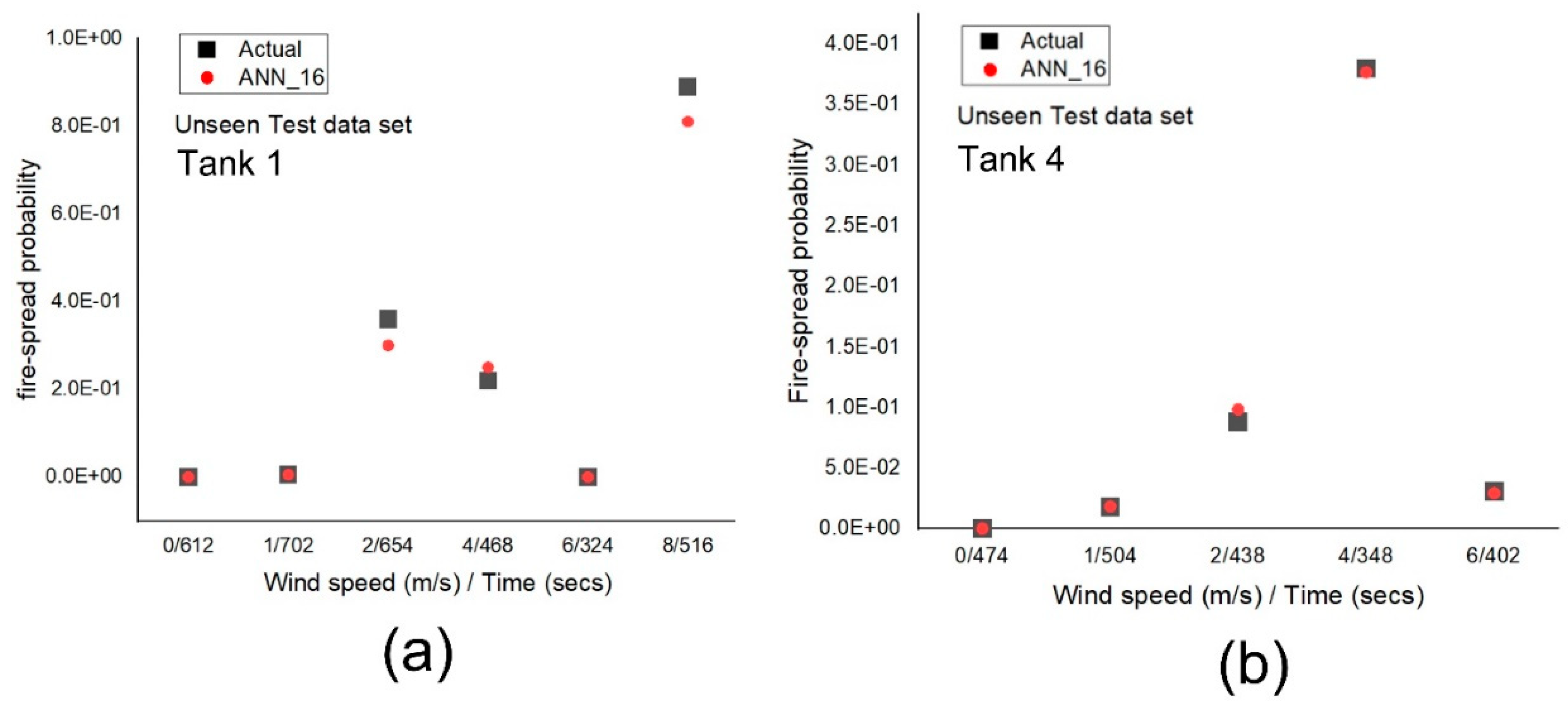
3.5. ANN-Based Fire Spread Probability Prediction against Unseen Data

As discussed earlier, ANN shows agreeing fire spread probabilities at all the wind speeds for the trained data set. The ANN prediction capability is also tested on the unseen validation data set as shown in Figure 20. It is seen from Figure 20 that ANN shows conforming results for the unseen validation data set. Furthermore, the performance indices of the ANN model for the unseen data set are presented in

Table 8. Performance indices of ANN for unseen data set (Tank 1 and Tank 4).

	Tank 1				Tank 4
Performance index	RMSE	MAE	MRE	R2	RMSE	MAE	MRE	R2
ANN	0.05	0.04	0.04	0.98	0.0006	0.0005	0.004	0.98

. It is seen that the fire spread probability values predicted by ANN conform with the unseen CFD-based calculation data. However, the R-squared correlation value for the unseen data is reduced slightly. This is because the model is tested against the values not included in the training data set. However, the R-squared value of 0.98 is still showing a good fit and justifying the model accuracy [74]. Arshad et al. [58] recently developed a well-tuned ANN model for dust ignition predictive modelling, and their R-squared correlation range of values for training data set are similar to our achieved R-squared values and the value slightly reduced for testing data set such as what observed in this study as well.

Hence, utilizing CFD to obtain the dynamic escalation probability and then integrating the data with ANN showed robustness in predicting transient fire spread probability at any time instant within the tank farm failure time for considered wind speeds for seen and unseen data set. This predictive technique, in addition to being convenient in application, could provide timely detection in the fire spread probability with respect to time so that the mitigation team could act accordingly.

From the results presented, it could be concluded that dynamic escalation probability can be used to predict the most vulnerable tanks in a tank farm that could trigger a domino effect. The determined vulnerable tanks can be optimally fire-protected to reduce the risk of tank farm fire spread. Moreover, this study gives a meso-level risk of fire spread probability in tank farms based on micro-level dynamic escalation probability of individual tanks.

The dynamic fire spread probability was predicted using ANN in this study, and it was discovered that ANN could be utilized reliably for dynamic probability predictions because it displayed conformance with the unseen data. The optimized ANN model developed in this work might be employed to predict the dynamic fire spread probability precisely using data from any credible source. This ANN model can be further extended to be used for estimating dynamic fire spread probability in various other tank farm configurations and different weather conditions. In industries, it can be utilized to accurately anticipate the dynamic fire spread probability in a tank farm at a particular wind speed and time instant which can assist in fire safety and risk management. This research developed a method that integrates the fire spread probability results from advanced CFD simulation in data-driven predictive modelling using ANN. This study proved the reliability of ANN in predicting fire spread probabilities within substantially less computational time compared to CFD simulations. Since probability data of any reliable source can be used in this method, the developed ANN model could be useful in industrial applications where time management is a concern. The current ANN model is designed specifically for these tank farm cases, and its generalizability can be improved further in later research.

As mentioned above, incident heat flux is considered as the main parameter to cause the tank to fail. However, it is worth mentioning that including adiabatic surface temperature (AST) at the tanks in FDS modeling could also be a valuable parameter in investigating the transient thermal analysis of the tank shells including fuel autoignition which could be considered in future research.

4. Conclusions

This study performed fire propagation analysis in a tank farm using FDS with variable wind speeds and primary pool fire locations. Overall, it is found that wind speed above 1 m/s plays a significant role in the dynamic escalation of fires in a tank farm, and emergency response teams should take this into account when planning. The tanks which are in line with the wind direction and primary fire are the most susceptible with increasing wind speeds. The study found that as wind speed increases from 2 m/s to 8 m/s, the failure time of inline tanks decreased greatest by 84% and the dynamic fire spread probability increased by triple orders. However, for a cornered primary fire, the overall tank farm failure time and fire spread probability differences were not much significant after 4 m/s. The location of the initial fire also plays a role, with a primary fire in the middle of the tank farm (Tank 4) resulting in a 20% earlier escalation of fire spread compared to the one with corned tank (Tank 1). The study also found that the escalation probability threshold of 10⁻⁵ is met about 50% earlier with higher wind speeds compared to windless conditions.

The dynamic fire spread probability obtained in this study can help fire safety practitioners and emergency response planners estimate the critical period when the dynamic fire spread probability is unacceptable under specific wind conditions. The ANN model predicts the fire spread probability at each time instant within the tank farm failure and wind speed range using CFD simulation and dynamic escalation calculations. Fire safety engineers can employ semi-empirical models and CFD-based computations to obtain fire spread probability data for the ANN model. CFD provides more accurate fire spread probabilities, especially in windy conditions. The modelling showed that ANN accurately predicts fire spread risk at all wind speeds and times during tank farm failure.