Wildfire Risk Zone Mapping in Contrasting Climatic Conditions: An Approach Employing AHP and F-AHP Models

Abstract

Wildfires are one of the gravest and most momentous hazards affecting rich forest biomes worldwide; India is one of the hotspots due to its diverse forest types and human-induced reasons. This research aims to identify wildfire risk zones in two contrasting climate zones, the Wayanad Wildlife Sanctuary in the Western Ghats and the Kedarnath Wildlife Sanctuary in the Himalayas, using geospatial tools, analytical hierarchy process (AHP), and fuzzy-AHP models to assess the impacts of various conditioning factors and compare the efficacy of the two models. Both of the wildlife sanctuaries were severely battered by fires in the past, with more than 100 fire incidences considered for this modeling. This analysis found that both natural and anthropogenic factors are responsible for the fire occurrences in both of the two sanctuaries. The validation of the risk maps, utilizing the receiver operating characteristic (ROC) method, proved that both models have outstanding prediction accuracy for the training and validation datasets, with the F-AHP model having a slight edge over the other model. The results of other statistical validation matrices such as sensitivity, accuracy, and Kappa index also confirmed that F-AHP is better than the AHP model. According to the F-AHP model, about 22.49% of Kedarnath and 17.12% of Wayanad fall within the very-high risk zones. The created models will serve as a tool for implementing effective policies intended to reduce the impact of fires, even in other protected areas with similar forest types, terrain, and climatic conditions.

1. Introduction

Wildfires, blazes, and smoldering forest cover are among the most frequent natural catastrophes, causing significant loss of natural resources in addition to human loss. According to the EM-DAT portal (https://public.emdat.be/ (accessed on 16 October 2022)), the 10 most impacted countries recorded 2851 total wildfire-related fatalities between 1900 and 2022. However, things are not different in other countries. According to the study by Reddy et al. [1], India has the second-highest emerging forest fire hotspot areas among the seven South Asian nations for both natural and human-caused reasons [2]. Lightning [2], volcanic eruption [3,4], friction exerted by rolling stones, dry bamboo stalks rubbing against one another [5], and, in the most extreme cases, a meteorite or asteroid impact [6] are all natural sources of wildfires. Changes in the climate and weather can make wildfires worse [7]. During the dry summer months, evaporation of soil moisture increases, which causes an increase in flammable vegetation that might initiate wildfires [8]. Additionally, due to climate change and the associated lengthened duration of high temperatures, the fire season is getting extended. Since a few years ago, there has been a significant increase in the worldwide surface wind speed, a facilitator for forest fires, and this change is caused by ocean–atmosphere oscillations, such as El Niño events, which were also linked to climate change [9,10]. According to climate change projections, the temperature differential between land and water will increase, which will enhance wind characteristics in tropical and southern subtropical regions in the future [11]. Wildfires may receive more oxygen from strong winds, which would accelerate their spread [8]. Future projections show that as climate change gets worse the risk of wildfires will continue to rise in several parts of the world [12,13,14,15]. Accidental and intentional reasons are among the causes of anthropogenic wildfires [5].

According to Cieslik et al. [16], wildfires can cause the emission of greenhouse gases and pollutants such as VOCs, NH₃, CO, SOx, and NOx, and diminish organic carbon levels in the soil. It can affect the physico-chemical and ecological states of water systems, alter carbon storage and vegetation [17], and increase the local land surface temperature [18,19,20]. A map depicting wildfire risk zones is, therefore, necessary to pinpoint the critical areas and put in place efficient mitigation strategies. The likelihood that a fire would initiate is referred to as “fire risk” and is based on the existence and activity of the causative factors [21].

The climate is an important parameter in the initiation of forest fires and a decisive factor in prolonging forest fires. A comparative study is quintessential to understanding the differences in different climatic zones. Hence, the foremost aim of this study is to carry out a study in two extreme climatic conditions. India, a country with diverse physiographic, geomorphic, and climatic zones, thus, became the clear choice. The best regions of study are those where the interplay of natural and anthropogenic factors exists. Thus, both a wildlife sanctuary resting in the subtropical humid climate (Cwg of Koppen’s classification), i.e., the Kedarnath Wildlife Sanctuary (KWLS) in the foothills of the Himalayas, and one in the tropical monsoonal climate (Amw of Koppen’s classification), i.e., the Wayanad Wildlife Sanctuary (WWLS) in the Western Ghats, were selected for this study. However, the question of which techniques to adopt is also a matter of concern. Researchers applied models such as AHP [22], Fuzzy-AHP (F-AHP) [23], frequency ratio [24], fuzzy logic [25], logistic regression [26], artificial neural network (ANN) [26], analytical network process [25], support vector machine (SVM) [27], naïve Bayes [28], random forest [29], and decision tree [27] for mapping wildfire risk zones. AHP sorts and compares variables based on their entities and categorizes them into hierarchies or groups [30]. By simplifying, dividing, and comparing many variables, the AHP reduces cognitive errors, and it can compare both quantitative and qualitative indicators [30]. AHP can handle judgement situations involving numerous decision-makers, subjective assessments, and the ability to provide metrics of consistency of choice [31,32]. F-AHP is used to address AHP’s inability to manage evaluation subjectivity and ambiguity [33]. In addition, AHP and F-AHP will also perform better than machine learning techniques in situations where there is insufficient data [34,35].

Though many researchers employed the AHP model for the demarcation of wildfire risk zones [22,24,36,37,38,39,40,41,42,43,44,45,46], only a few researchers attempted the F-AHP model [23,47,48,49,50,51]. Tiwari et al. [52] applied the AHP, F-AHP, and frequency ratio models for modelling forest fire susceptibility in Pauri Garhwal (India). However, so far, the AHP and F-AHP models have never been compared for wildfire risk modeling. The AHP and F-AHP models have been compared only for assessing the efficacy of landslide susceptibility [53,54], flood susceptibility [55,56], flood vulnerability [57], and forest fire susceptibility [52]. This is the uniqueness of this study, as no researchers have assessed the prediction capability of both the AHP and F-AHP models for the demarcation of wildfire risk zones and applied different models for the comparison of two protected areas with different vegetation in any part of the world. Furthermore, the influence of mass gathering sites such as major tourist spots and pilgrim/religious centers has not yet been assessed in any of the published works. Considering the presence of rich and unique flora and fauna in the sanctuaries, this study has a crucial role to play in minimizing the threats posed by wildfires.

Thus, the purposes of this modelling are to: (a) demarcate the wildfire risk zones in two contrasting climate zones, in this case the Kedarnath Wildlife Sanctuary and Wayanad Wildlife Sanctuary, using the AHP and F-AHP models; (b) compare the influence of conditioning factors (land cover types, slope, Land Surface Temperature, normalized difference water index, distance from the road, distance from the major tourist spot and pilgrim/religious center, distance from the settlement, Water Ratio Index, and normalized difference built-up index) on fire occurrence and spread in the two wildlife sanctuaries; and (c) compare the prediction capability of the two models for both wildlife sanctuaries.

2. Materials and Methods

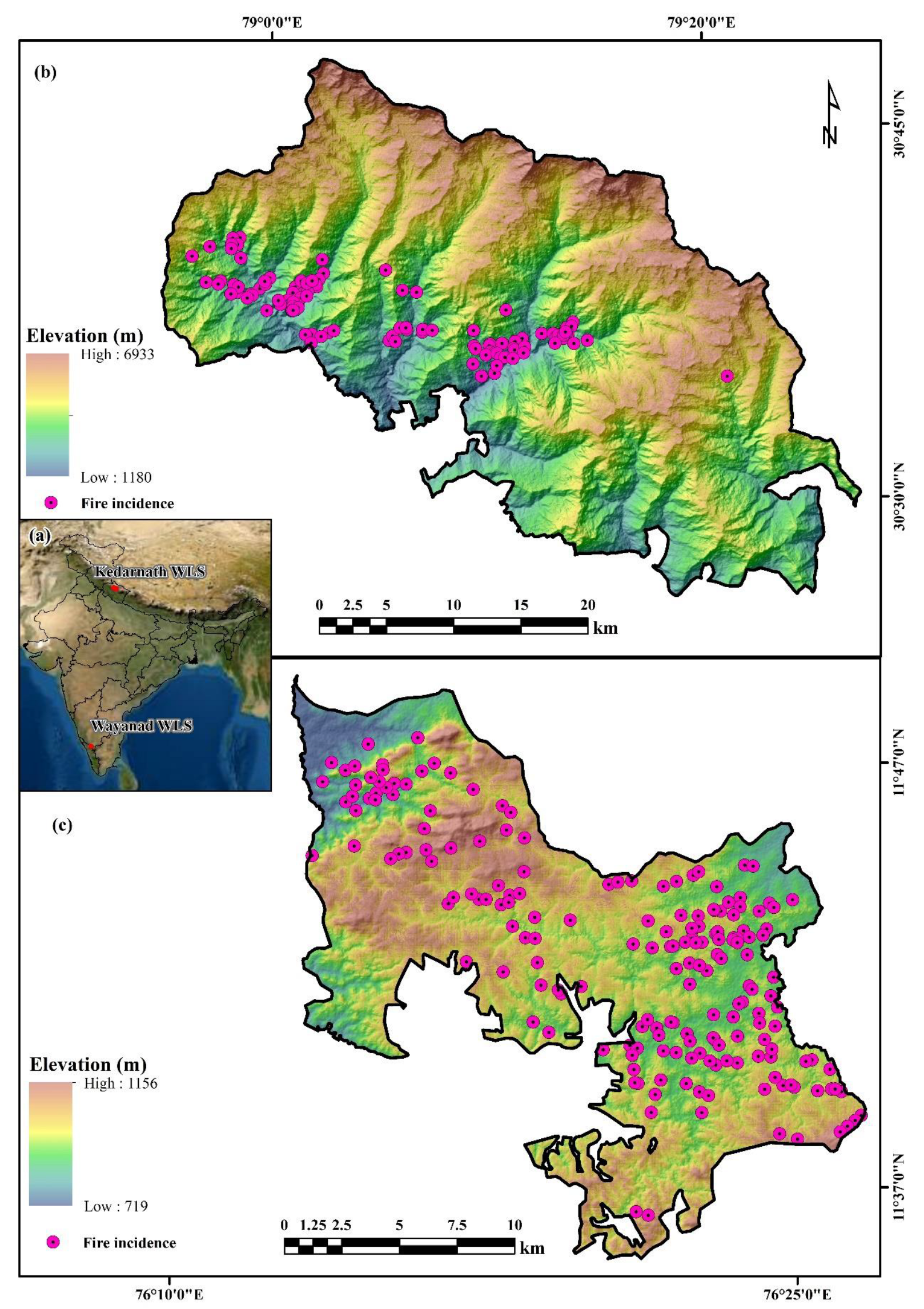
2.1. Study Area

2.1.1. Kedarnath Wildlife Sanctuary (KWLS)

The KWLS, in the Uttarakhand districts of Chamoli and Rudraprayag (i.e., the Garhwal Himalayas), is one of the largest protected areas (975 km²) [58]. The Himalayan mountains, such as Chaukhamba (7068 m), Kedarnath (6940 m), and Mandani (6193 m), surround the sanctuary and are situated in the upper catchment area of the Alaknanda and Mandakini Rivers, both of which are the main tributaries of the Ganges [59,60]. The sanctuary usually remains covered in snow for almost three months during the winter [61]. Even in low-altitude locations, there will be moderate to severe snowfall from December through February [59]. The region experiences 3000 mm of annual rainfall, of which roughly 60% occurs between June and August during the monsoon season [59]. The mean maximum temperature ranges from 4 °C to 33.5 °C [59].

The forests are mainly dominated by different tree species, viz., West Himalayan fir (Abies pindrow), East Himalayan fir (Abies spectabilis), Deodar cedar (Cedrus deodara), Himalayan or Bhutan cypress (Cupressus torulosa), English walnut (Juglans regia), Common juniper (Juniperus communis), Himalayan bayberry (Myrica esculenta), Chir pine (Pinus roxburghii), Bhutan pine (Pinus wallichiana), Banj oak (Quercus leucotrichophora), Japanese blue oak (Quercus glauca), Green oak (Quercus floribunda), Brown oak (Quercus semecarpifolia), Rhododendron (Rhododendron arboretum), Yellow-paint maple (Acer pictum), Indian or Himalayan horse-chestnut (Aesculus indica), Himalayan birch (Betula utilis), Nepalese alder (Alnus nepalensis), Common yew (Taxus Baccata), Indian tees (Aconitum heterophyllum), Fading Himalayan aster (Aster albescens), Himalayan cinquefoil (Potentilla fulgens), Drumstick primula (Primula denticulate), English primrose (Primula stuartii), and Common dandelion (Taraxacum officinale) [62,63]. The Himalayan tahr (Hemitragus jemlahicus), Himalayan musk deer (Moschus leucogaster), Himalayan goral (Naemorhedus goral), Serow (Capricornis sumatraensis), Barking deer (Muntiacus muntjak), Sambar (Cervus unicolor), and Wild boar (Sus scrofa) are the noteworthy fauna of this sanctuary [63].

2.1.2. Wayanad Wildlife Sanctuary (WWLS)

A major protected area of the Nilgiri Biosphere Reserve of the Western Ghats is the WWLS. This sanctuary is bordered by the national parks of Bandipur and Nagarhole in Karnataka, as well as Mudumalai in Tamil Nadu [64]. The WWLS covers a 344.44 km² area and is divided into two distinct units measuring 77.67 km² (the northern portion) and 266.77 km² (the southern portion). This sanctuary comprises the Sulthan Bathery, Muthanga, Tholpetty, and Kurichiat forest ranges. The Tholpetty range is located in the northern segment, while the other three forest ranges are located in the southern segment [65,66,67]. The major river traversing the sanctuary is the Kabani [64]. According to Arjun et al. [65], the annual rainfall at the WWLS is between 3000 and 4000 mm, and the average temperature is between 13 and 32 °C [67].

The WWLS is home to the largest remaining population of Asiatic elephants (Elephas maximus) [65] and also to Tigers (Panthera tigris), Leopards (Panthera pardus), Gaurs (Bos gaurus), Wild boars (Sus scrofa), Spotted deer (Axis axis), Barking deer (Muntiacus muntjak), Sambars (Rusa unicolor), Sloth bears (Melursus ursinus), Bonnet macaques (Macaca radiata), Nilgiri langurs (Semnopithecus johnii), Common otters (Lutra Lutra), and Malabar giant squirrels (Ratufa indica) [67]. The major tree species include Teak (Tectona grandis), damson (Terminalia spp.), Indian rosewood (Dalbergia latifolia), axle-wood (Anogeissus latifolia), Dhaman (Grewia tiliaefolia), Haldu (Adina cordifolia), Cinnamon (Cinnamomum zeylanicum), Indian kino (Pterocarpus marsupium), white dammar (Vateria indica), Cebuano (Lagerstroemia lanceolata), Wild jack (Artocarpus hirsutus), and Chandada (Macaranga peltate) [67]. In this study, only the southern portion of the WWLS is considered, as the northern portion is a geographically isolated place (Figure 1).

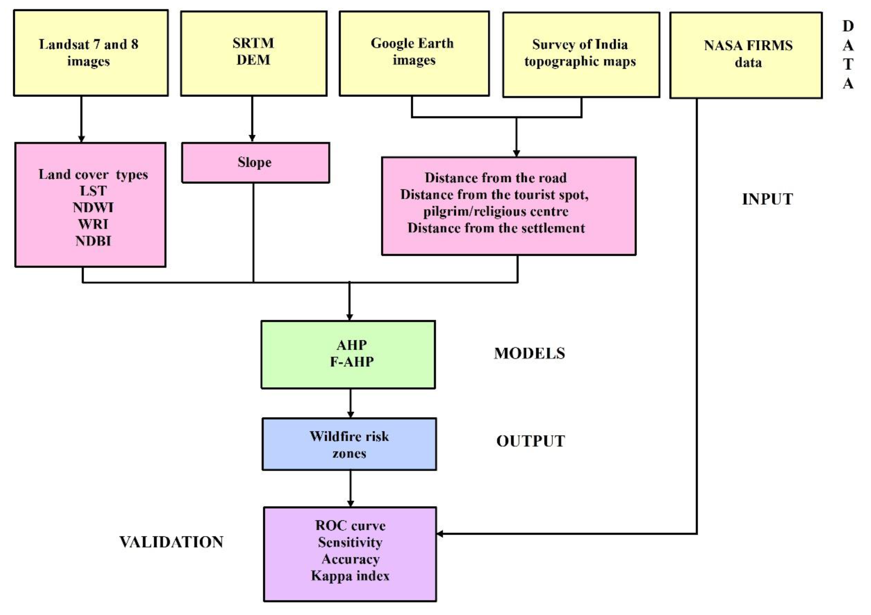
2.2. Data Source and Major Steps

The following were the six major steps involved:

1.

Data were gathered from a variety of sources; both primary and secondary (

Table 1. Data source.

Data	Source	Layers Derived (Factor)	Scale	Spatial Resolution
Landsat 8 OLI image	https://earthexplorer.usgs.gov/ (accessed on 21 September 2022)	Land cover types NDWI WRI NDBI		30 m
Landsat 7 ETM+	https://earthexplorer.usgs.gov/ (accessed on 21 September 2022)	LST		60 m
Landsat 8 TIRS image	https://earthexplorer.usgs.gov/ (accessed on 21 September 2022)	LST		100 m
SRTM DEM	https://earthexplorer.usgs.gov/ (accessed on 5 January 2020)	Slope		30 m
Topographic map	Survey of India	Distance from the road Distance from the tourist spot, pilgrim/religious center Distance from the settlement	1: 50,000
Google Earth Pro	https://earth.google.com/web/ (accessed on 5 October 2022)	Distance from the road (updated) Distance from the tourist spot, pilgrim/religious center (updated) Distance from the settlement (updated)		15 cm to 15 m
NASA FIRMS data	https://firms.modaps.eosdis.nasa.gov/download/ (accessed on 27 July 2022)	Fire incidence points		375 m (VIIRS) and1 km (MODIS)

). ArcGIS 10.8 (Esri, Inc., Redlands, CA, USA) and ERDAS Imagine 9.2 (Hexagon AB, Stockholm, Sweden) were used to create the thematic layers for these different factors.

2.

The layers of continuous factors such as the slope, Land Surface Temperature (LST), Normalized Difference Water Index (NDWI), distance from the road, distance from the major tourist spot and pilgrim/religious center, distance from the settlement, Water Ratio Index (WRI), and Normalized Difference Built-up Index (NDBI) were classified using the Natural breaks method [57,68].

3.

The multicollinearity of factors was tested employing the Variance Inflation Factor (VIF) and tolerance.

4.

The risk zone maps were created employing the AHP and F-AHP models. MS Excel and FisPro 3.8 (https://www.fispro.org/en/ (accessed on 11 August 2022)) [69,70] were employed to derive the weights of the AHP and F-AHP models, respectively (Figure 2).

5.

The Fire Radiative Power [71,72] distribution of the fire events has been plotted to assess the characteristics of wildfires. This data has been retrieved from the FIRMS portal.

6.

The risk zone maps were validated utilizing the ROC curve method and other statistical validation matrices such as sensitivity, accuracy, and Kappa index, and the R 4.2.1 (The R Foundation for Statistical Computing, Vienna, Austria) software was employed for the validation of the maps.

2.3. Creation of Wildfire Inventory

The fire incidence data for the period of 1 November 2000–26 July 2022 has been collected from NASA’s Fire Information for Resource Management System (FIRMS) portal (https://www.earthdata.nasa.gov/learn/find-data/near-real-time/firms (accessed on 27 July 2022)). Two satellite-derived fire incidence datasets are available within this portal, i.e., the Moderate Resolution Imaging Spectroradiometer (MODIS) and the Visible Infrared Imaging Radiometer Suite (VIIRS). This study utilized both MODIS and VIIRS data. As per the portal, a total of 124 wildfire incidences have been reported in the KWLS during this period, whereas the total incidence in the WWLS was 192.

2.4. Derivation of Conditioning Factors

The land cover types were extracted from the Landsat 8 images using the ERDAS Imagine software, and the maximum likelihood classification approach [73,74,75] was employed for this. The slope was determined from the DEM using the ArcGIS surface (spatial analyst) tool. The road networks, tourist spots, pilgrim/religious centers, and settlements were derived from the topographic maps and Google Earth Pro images employing ArcGIS tools. The distance from the road, the distance from the tourist spot and pilgrim/religious center, and the distance from the settlement layers were computed using the ArcGIS spatial analyst (Euclidean distance) tool.

Landsat 8 Thermal Infrared Sensor (TIRS) and Landsat 7 ETM+ images were utilized to derive the LST of the sanctuaries. The steps involved with the extraction of the LST are listed below:

i.

Transformation of the Digital Number (DN) to Spectral Radiance (Lλ)

Spectral radiance ($L_{\lambda }$) was computed employing Equation (1) [76].

$$L_{\lambda }=LMI{N}_{\lambda }+\left[\frac{\left(LMA{X}_{\lambda }-LMI{N}_{\lambda }\right)}{QCALMAX-QCALMIN}\times QCAL\right]$$

(1)

where QCAL = DN of pixels; QCALMAX = 255; QCALMIN = 0; $LMI{N}_{\lambda }$= spectral radiance at DN = 0; $LMA{X}_{\lambda }$= spectral radiance at DN = 255 [77].

ii.

Transformation of Spectral Radiance to At-Satellite Brightness Temperatures

Based on the type of land cover, the emissivity (e) for radiant temperatures has been rectified. Vegetation areas were given a score of 0.95, while unwooded areas were given a score of 0.92 [78]. As mentioned in Artis and Carnahan [79], the emissivity-corrected LST was identified (Equation (2)).

$$T_B=\frac{K_2}{\ln \left(\frac{K_1}{L_{\lambda }}\right)+1}$$

(2)

where $L_{\lambda }$ is Spectral Radiance in W.m⁻².sr⁻¹.μm⁻¹, and K₁ and K₂ are two constants [77].

iii.

LST Estimation

The spectral emissivity (ϵ) needs correction since the black body is denoted by the temperature values obtained from the above analyses. Rectification can be performed by rendering the land cover type or by computing the corresponding NDVI emissivity values for the respective pixels [80]. The rectified emissivity of the LST was determined using Equation (3) [79].

$$LST=\raisebox{1ex}{$T_B$}\!\left/ \!\raisebox{-1ex}{$\left[1+\left\{\left(\frac{\lambda \times T_B}{\rho }\right)\times ln\in \right\}\right]$}\right.$$

(3)

where the LST = LST in kelvin, $T_B$ = At-sensor brightness temperature, λ = TOA reflectance, and Inϵ = Emissivity [77].

Land surface emissivity was computed employing Equation (4).

$$Land surface emissivity \left(\in \right)=0.004\times p_v+0.986$$

(4)

where$p_v$ is the vegetation proportion, which was calculated using Equation (5) [77].

$$p_v={\left(\frac{NDV{I}_{jr}-NDV{I}_{min}}{NDV{I}_{max}-NDV{I}_{min}}\right)}^2$$

(5)

iv.

Conversion of Kelvin to Degree Celsius

The measurement unit of the predicted LSTs was transformed to a kelvin scale using the calculation 0 °C = 273.15 K to simplify the conceptualizing.

The NDWI was extracted from the Landsat images using the ArcGIS map algebra tool and Equation (6) [81]. The WRI was computed from the satellite images using the ArcGIS map algebra tool and Equation (7) [82]. The ArcGIS map algebra tool and Equation (8) [83] were utilized to derive the NDBI values.

$$NDWI=\frac{\left(Green-NIR\right)}{\left(Green+NIR\right)}$$

(6)

$$WRI=\frac{\left(Green+Red\right)}{\left(NIR+SWIR\right)}$$

(7)

$$NDBI=\frac{\left(SWIR-NIR\right)}{\left(SWIR+NIR\right)}$$

(8)

where Green, Red, NIR, and SWIR denote spectral reflectance measurements in the Green, Red, Near infrared, and Short-wave infrared bands, respectively.

2.5. Multi-Collinearity Test

Anytime an independent factor in a multivariate regression equation has a high correlation with one or more additional independent factors, multicollinearity exists [84,85]. The standard error will be relatively substantial for an independent factor with a high correlation to one or more other independent factors [84]. The Variance Inflation Factor (VIF) and tolerance are the most widely employed measures of the degree of multi-collinearity [86]. The VIF shows how strongly a variable’s linear relationship to the other explanatory factors is [87]. According to Ferré [88], a VIF larger than 10 indicates that the correlation (collinearity) between the factors is so high that the standard error of the regression coefficient is excessively increased. The reciprocal of the VIF is known as the tolerance, and if the tolerance is lower than 0.1 to 0.2, multicollinearity exists [89]. The VIF was computed employing Equation (9) [87].

$$VI{F}_j=\frac{1}{1-R^2{}_j}$$

(9)

where$R^2{}_j$ is the ${\mathrm{R}}^2$ from the regression of the j^th explanatory factor on the remaining explanatory factors.

2.6. AHP Modeling

Saaty’s AHP [90] is a well-known and frequently applied multi-criteria decision-making technique [91,92]. The AHP method’s blending of qualitative and quantitative analysis is one of its hallmarks [93]. The important relationship between each factor is quantitatively stated by combining expert judgment with objective assessment, and a matrix of the various conditioning factors will be created [93]. The capacity to gauge consistency is another benefit of the AHP model [33]. The critical stages in the AHP modelling process are the creation of the matrix for pair-wise comparisons, the determination of the Eigenvector, the weighting coefficient (

Table 2. Pairwise comparison matrix.

	LCT	Slp	LST	NDWI	DR	DTSPRC	DS	WRI	NDBI	Vp	Cp
LCT	1	2	3	4	5	6	7	8	9	4.147	0.308
Slp	1/2	1	2	3	4	5	6	7	8	3.008	0.223
LST	1/3	1/2	1	2	3	4	5	6	7	2.113	0.157
NDWI	1/4	1/3	1/2	1	2	3	4	5	6	1.459	0.108
DR	1/5	1/4	1/3	1/2	1	2	3	4	5	1.000	0.074
DTSPRC	1/6	1/5	1/4	1/3	1/2	1	2	3	4	0.685	0.051
DS	1/7	1/6	1/5	1/4	1/3	1/2	1	2	3	0.473	0.035
WRI	1/8	1/7	1/6	1/5	1/4	1/3	1/2	1	2	0.332	0.025
NDBI	1/9	1/8	1/7	1/6	1/5	1/4	1/3	1/2	1	0.241	0.018
∑	2.83	4.72	7.59	11.45	16.28	22.08	28.83	36.50	45.00	13.46	1.00

Where LCT = Land cover types, Slp = Slope, DR = Distance from the road, DTSPRC = Distance from the tourist spot and pilgrim/religious center, and DS = Distance from the settlement.

), and the consistency ratio (

Table 3. Normalized matrix.

	LCT	Slp	LST	NDWI	DR	DTSPRC	DS	WRI	NDBI	∑rank	[C]	[D] = [A]*[C]	[E] = [D]/[C]	λmax	CI	CR
LCT	0.35	0.42	0.40	0.35	0.31	0.27	0.24	0.22	0.20	2.76	0.307	2.981	9.711	9.408	0.051	0.035 (3.52%)
Slp	0.18	0.21	0.26	0.26	0.25	0.23	0.21	0.19	0.18	1.96	0.218	2.134	9.782
LST	0.12	0.11	0.13	0.17	0.18	0.18	0.17	0.16	0.16	1.39	0.154	1.499	9.715
NDWI	0.09	0.07	0.07	0.09	0.12	0.14	0.14	0.14	0.13	0.98	0.109	1.040	9.548
DR	0.07	0.05	0.04	0.04	0.06	0.09	0.10	0.11	0.11	0.69	0.076	0.714	9.345
DTSPRC	0.06	0.04	0.03	0.03	0.03	0.05	0.07	0.08	0.09	0.48	0.053	0.489	9.168
DS	0.05	0.04	0.03	0.02	0.02	0.02	0.03	0.05	0.07	0.33	0.037	0.336	9.077
WRI	0.04	0.03	0.02	0.02	0.02	0.02	0.02	0.03	0.04	0.23	0.026	0.236	9.104
NDBI	0.04	0.03	0.02	0.01	0.01	0.01	0.01	0.01	0.02	0.17	0.019	0.174	9.222
∑	1.00	1.00	1.00	1.00	1.00	1.00	1.00	1.00	1.00	9.00	1.000		84.672

) [53,57].

Equations (10) and (11) were employed to determine the Eigenvector (Vp) and weighting coefficient (Cp) [22,53,94]:

$$Vp=\sqrt[k]{W1\times \dots Wk}$$

(10)

where k = no. of factors, and W = ratings,

$$Cp=\frac{Vp}{Vp1+\dots Vpk}$$

(11)

As explained by Danumah et al. [95], the normalized matrix, priority vector [C], overall priority [D], and rational priority [E] were computed. Equations (12)–(14) were employed to calculate the eigenvalue (λmax), consistency index (CI), and consistency ratio (CR) [22,53,94].

$$\lambda max=\frac{\left[E\right]}{k}$$

(12)

$$CI=\raisebox{1ex}{$\left(\lambda max-k\right)$}\!\left/ \!\raisebox{-1ex}{$\left(k-1\right)$}\right.$$

(13)

$$CR=\frac{CI}{RI}$$

(14)

where (RI) random index = 1.49 [90].

Saaty [90] recommends a consistency ratio (CR) of less than 0.1. The analysis has to be repeated if the CR is larger than 0.1. The AHP modelling in this study yields an acceptable CR of 0.035. As a result, the results can be relied upon.

The AHP weights are depicted in Equation (15).

$$\begin{gathered} FRZ=\left(0.308\times LCT\right)+\left(0.223\times Slp\right)+\left(0.157\times LST\right)+\left(0.108\times NDWI\right)+\left(0.074\times DR\right) \\ +\left(0.051\times DTSPRC\right)+\left(0.035\times DS\right)+\left(0.025\times WRI\right)+\left(0.018\times NDBI\right) \end{gathered}$$

(15)

2.7. F-AHP Modelling

F-AHP [96], an AHP method developed by utilizing fuzzy logic theory [97], was established to solve the scenario wherein experts struggle to render an accurate comparative assessment [98]. Typically, a set of triangular fuzzy numbers (TFN) are used to develop the F-AHP [98]. The F-AHP is the best choice for resolving the issue of null weights for factors and scores for alternatives without compromising the consistency of the outcomes [99]. The ease of computing implementation and the improved capability to discern the significance of the factors when the weights are close are additional advantages of this method [99]. Discrepancies can occur during the development of pairwise comparisons in the AHP model [100]. However, this can be solved by employing the F-AHP approach [101]. For comparing the fuzzy ratios, Buckley’s [102] method was utilized. The crucial stages include creating a pair-wise comparison matrix (

Table 4. Pairwise comparison of factors.

	LCT	Slp	LST	NDWI	DR	DTSPRC	DS	WRI	NDBI
LCT	(1, 1, 1)	(1, 2, 3)	(2, 3, 4)	(3, 4, 5)	(4, 5, 6)	(5, 6, 7)	(6, 7, 8)	(7, 8, 9)	(9, 9, 9)
Slp	(1/3, 1/2, 1)	(1, 1, 1)	(1, 2, 3)	(2, 3, 4)	(3, 4, 5)	(4, 5, 6)	(5, 6, 7)	(6, 7, 8)	(7, 8, 9)
LST	(1/4, 1/3, 1/2)	(1/3, 1/2, 1)	(1, 1, 1)	(1, 2, 3)	(2, 3, 4)	(3, 4, 5)	(4, 5, 6)	(5, 6, 7)	(6, 7, 8)
NDWI	(1/5, 1/4, 1/3)	(1/4, 1/3, 1/2)	(1/3, 1/2, 1)	(1, 1, 1)	(1, 2, 3)	(2, 3, 4)	(3, 4, 5)	(4, 5, 6)	(5, 6, 7)
DR	(1/6, 1/5, 1/4)	(1/5, 1/4, 1/3)	(1/4, 1/3, 1/2)	(1/3, 1/2, 1)	(1, 1, 1)	(1, 2, 3)	(2, 3, 4)	(3, 4, 5)	(4, 5, 6)
DTSPRC	(1/7, 1/6, 1/5)	(1/6, 1/5, 1/4)	(1/5, 1/4, 1/3)	(1/4, 1/3, 1/2)	(1/3, 1/2, 1)	(1, 1, 1)	(1, 2, 3)	(2, 3, 4)	(3, 4, 5)
DS	(1/8, 1/7, 1/6)	(1/7, 1/6, 1/5)	(1/6, 1/5, 1/4)	(1/5, 1/4, 1/3)	(1/4, 1/3, 1/2)	(1/3, 1/2, 1)	(1, 1, 1)	(1, 2, 3)	(2, 3, 4)
WRI	(1/9, 1/8, 1/7)	(1/8, 1/7, 1/6)	(1/7, 1/6, 1/5)	(1/6, 1/5, 1/4)	(1/5, 1/4, 1/3)	(1/4, 1/3, 1/2)	(1/3, 1/2, 1)	(1, 1, 1)	(1, 2, 3)
NDBI	(1/9, 1/9, 1/9)	(1/9, 1/8, 1/7)	(1/8, 1/7, 1/6)	(1/7, 1/6, 1/5)	(1/6, 1/5, 1/4)	(1/5, 1/4, 1/3)	(1/4, 1/3, 1/2)	(1/3, 1/2, 1)	(1, 1, 1)

), computing geometric means (

Table 5. Geometric mean.

	$\mathbf{Fuzzy} \mathbf{Geometric} \mathbf{Mean} \left({\tilde{\mathit{r}}}_{\mathit{i}}\right)$
LCT	3.292	4.147	4.902
Slp	2.282	3.008	3.840
LST	1.576	2.113	2.785
NDWI	1.080	1.459	1.956
DR	0.740	1.000	1.351
DTSPRC	0.511	0.685	0.926
DS	0.359	0.473	0.634
WRI	0.260	0.332	0.438
NDBI	0.204	0.241	0.304
$\sum {\tilde{r}}_i$	10.305	13.460	17.136
${\left(\sum {\tilde{r}}_i\right)}^{-1}$	0.058	0.074	0.097

), estimating relative fuzzy weights (

Table 6. Relative fuzzy weights.

	$\mathbf{Fuzzy} \mathbf{Weight} \left[{\tilde{\mathit{w}}}_{\mathit{i}}\mathbf{W}\right]$
LCT	0.192	0.308	0.476
Slp	0.133	0.223	0.373
LST	0.092	0.157	0.270
NDWI	0.063	0.108	0.190
DR	0.043	0.074	0.131
DTSPRC	0.030	0.051	0.090
DS	0.021	0.035	0.062
WRI	0.015	0.025	0.043
NDBI	0.012	0.018	0.029

), and calculating averaged and normalized relative weights (

Table 7. Normalized weights.

	$\mathbf{Weight} \left({\mathbf{M}}_{\mathbf{i}}\mathbf{Mi}\right)$	$\mathbf{Normalized} \mathbf{Weight} \left({\mathbf{N}}_{\mathbf{i}}\mathbf{Ni}\right)$
LCT	0.325	0.299
Slp	0.243	0.223
LST	0.173	0.159
NDWI	0.120	0.111
DR	0.083	0.076
DTSPRC	0.057	0.052
DS	0.039	0.036
WRI	0.027	0.025
NDBI	0.020	0.018
∑	1.09	1.00

) [53,57]. The following were the crucial steps in the F-AHP modelling process:

Step 1: The factors were compared.

The fuzzy triangular scale (1/4, 1/3, 1/2) will be utilized when factor 1 (P1) is of lower priority than factor 2 (P2). For the comparison matrix, the fuzzy triangular scale will be (1/4, 1/3, 1/2) [103].

Equation (16) depicts the matrix:

$${\tilde{A}}^k=\left[\begin{array}{ccc}{\tilde{d}}_{11}^k& {\tilde{d}}_{12}^k& \begin{array}{cc}\dots & {\tilde{d}}_{1n}^k\end{array}\\ \begin{array}{c}{\tilde{d}}_{21}^k\\ \dots \end{array}& \begin{array}{c}\dots \\ \dots \end{array}& \begin{array}{c}\begin{array}{cc}\dots & {\tilde{d}}_{2n}^k\end{array}\\ \begin{array}{cc}\dots & \dots \end{array}\end{array}\\ {\tilde{d}}_{n1}^k& {\tilde{d}}_{n2}^k& \begin{array}{cc}\dots & {\tilde{d}}_{mn}^k\end{array}\end{array}\right]$$

(16)

where${\widetilde{ d}}_{ij}^k$ reflects the k^th decision maker’s preference for the i^th factor over the j^th factor [103].

Step 2:${\tilde{d}}_{ij}$ was computed using Equation (17) [57]:

$${\tilde{d}}_{ij}=\frac{{{\displaystyle \sum }}_{k=1}^K{\tilde{d}}_{ij}^k}{K}$$

(17)

Step 3: Equation (18) was applied to transform the matrix [57]:

$$\tilde{A}=\left[\begin{array}{ccc}{\tilde{d}}_{11}& \cdots & {\tilde{d}}_{1n}\\ ⋮& \ddots & ⋮\\ {\tilde{d}}_{n1}& \cdots & {\tilde{d}}_{nn}\end{array}\right]$$

(18)

Step 4: Equation (19) [102] was employed to determine the geometric average:

$${\tilde{r}}_i={\left({\displaystyle \prod }_{j=1}^n{\tilde{d}}_{ij}\right)}^{\raisebox{1ex}{$1$}\!\left/ \!\raisebox{-1ex}{$n$}\right.}, i=1,2,\dots ,n$$

(19)

where${\widetilde{ r}}_i$= triangular values.

Step 5: From the following sub-steps (5a, 5b, and 5c), the fuzzy weights were computed.

Step 5a: Summation vector of each ${\tilde{r}}_i$ was determined.

Step 5b: After computing the summation vector’s (−1) power, the fuzzy triangular number was replaced to transform it into ascending order.

Step 5c: The fuzzy weight was determined by multiplying ${\tilde{r}}_i$ with the reverse vector as represented in Equations (20) and (21) [57]:

$${\tilde{w}}_i={\tilde{r}}_i\times {\left({\tilde{r}}_1+{\tilde{r}}_2+\dots +{\tilde{r}}_n\right)}^{-1}$$

(20)

$${\tilde{w}}_i=\left(l{w}_i,m{w}_i,u{w}_i\right)$$

(21)

Step 6: The fuzzy weights were de-fuzzified as in Equation (22) [104]:

$$M_i=\frac{l{w}_i,m{w}_i,u{w}_i}{3}$$

(22)

Step 7: Equation (23) was employed for the standardization of$M_i$ [57]:

$$N_i=\frac{M_i}{{{\displaystyle \sum }}_{i=1}^n{M}_i}$$

(23)

Equation (24) depicts the F-AHP weights:

$$\begin{gathered} FRZ=\left(0.299\times LCT\right)+\left(0.223\times Slp\right)+\left(0.159\times LST\right)+\left(0.111\times NDWI\right)+\left(0.076\times DR\right) \\ +\left(0.052\times DTSPRC\right)+\left(0.036\times DS\right)+\left(0.025\times WRI\right)+\left(0.018\times NDBI\right) \end{gathered}$$

(24)

2.8. Validation of the Maps

2.8.1. ROC Curve

The ROC method [36,53,68,94] was adopted to validate the created risk zone maps to assess the prediction capability. The ROC curve is a two-dimensional graph frequently used to determine the effectiveness of classifiers [105]. According to Hanley and McNeil [106], AUC is a single scalar metric that depicts a classifier’s overall efficacy. The least AUC value (0.5) denotes a random performance; whereas the highest score (1.0) denotes a perfect classifier [105]. The ROC curves were plotted, and the AUC values were computed using the R 4.2.1 software. The fire incidence data was employed to validate the results. This fire incidence data was divided into two datasets: training (70%) and validation (30%). In the case of the WWLS, the training dataset contained 133 fire incidence locations and the validation dataset contained 59 incidence locations, whereas the training dataset contained 87 locations, and the validation dataset contained 37 incidence locations for the KWLS. According to Li and He [107], an AUC value ranging between 0.50 and 0.60, 0.60 and 0.70, 0.70 and 0.80, 0.80 and 0.90, and 0.90 and 1.00 represents failure, poor, fair, good, and excellent performance.

2.8.2. Sensitivity and Accuracy

The sensitivity is the percentage of wildfires that were correctly identified by the test [108]. The degree to which a set of observations corresponds to their actual value is known as accuracy [109]. Sensitivity and specificity reflect the model’s robustness, while accuracy demonstrates the model’s predictivity [110]. Sensitivity and accuracy were computed using Equations (25) and (26) [111,112].

$$Sensitivity=\frac{TP}{TP+FN}$$

(25)

$$Accuracy=\frac{TP+TN}{TP+FP+FN+TN}$$

(26)

where TP, TN, FP, and FN are true positives, true negatives, false positives, and false negatives, respectively.

2.8.3. Kappa Index

Cohen’s Kappa index [113] measures the degree of agreement between a pair of factors [114] and is used to estimate interrater reliability [115,116]. The value ranges between −1 and 1, with 1 representing complete agreement, 0 representing no agreement, and a negative score representing worse agreement [114]. Kappa scores equal to or less than 0 indicate no agreement; 0.01–0.20 indicate slight to no agreement; 0.21–0.40 indicate fair; 0.41–0.60 indicate moderate; 0.61–0.80 indicate substantial agreement; and 0.81–1.00 indicate nearly perfect agreement [115]. The Kappa index was estimated using Equation (27) [117].

$$\mathrm{k}=\frac{P_{obs}-P_{exp}}{1-P_{exp}}$$

(27)

where$P_{obs}$ and $P_{exp}$ are observed and expected agreements, respectively.

3. Results

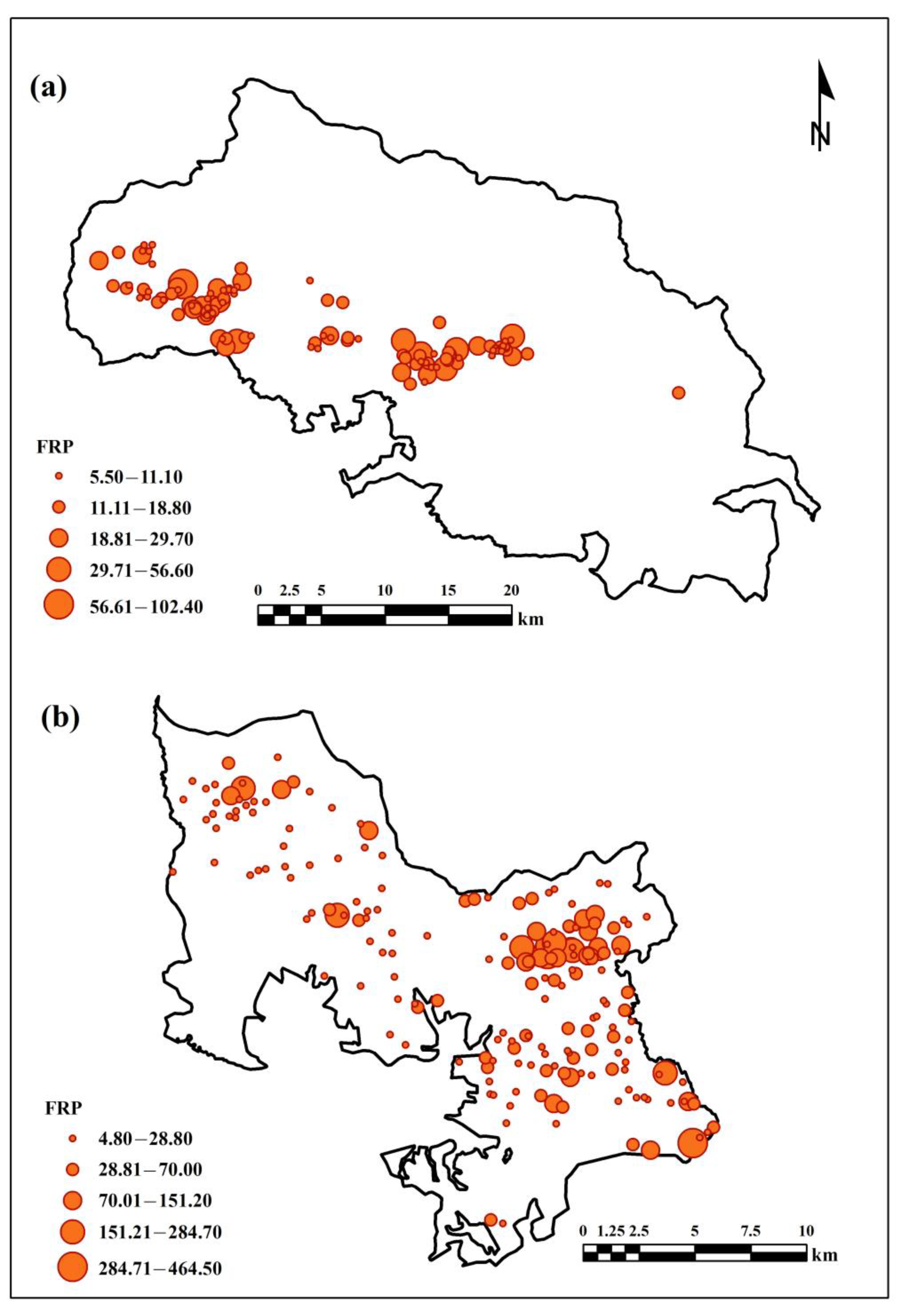
3.1. Fire Radiative Power (FRP) Distribution

The FRP, which is employed to quantify burned biomass [72,118], of the KWLS ranged from 5.50 to 102.40 MW, while the FRP of the WWLS ranged from 4.80 to 464.50 MW. The FRP distribution of fire events is depicted in Figure 3.

3.2. Multi-Collinearity Analysis

The multi-collinearity analysis confirmed that all factors were relevant, with tolerance values above 0.1 and VIF values below 5 (

Table 8. Multicollinearity analysis.

Factors	Collinearity Statistics of KWLS		Collinearity Statistics of WWLS
	Tolerance	VIF	Tolerance	VIF
LST	0.209	4.782	0.503	1.988
LCT	0.707	1.415	0.668	1.497
Slope	0.890	1.124	0.849	1.177
WRI	0.230	4.354	0.600	1.666
NDWI	0.288	4.472	0.593	1.687
Distance from the road	0.235	4.255	0.726	1.378
Distance from the tourist spot or pilgrim/religious center	0.576	1.735	0.881	1.135
Distance from the settlement	0.247	4.049	0.691	1.447
NDBI	0.278	3.597	0.772	1.295

). For the KWLS, the slope had the highest tolerance value (0.890), followed by the LCT, whereas for the WWLS the distance from the tourist spot or pilgrim/religious center had the highest tolerance value of 0.881, followed by the slope (0.849). The VIF of the KWLS ranged from 1.124 to 4.782, whereas the VIF of the WWLS ranged between 1.135 and 1.988.

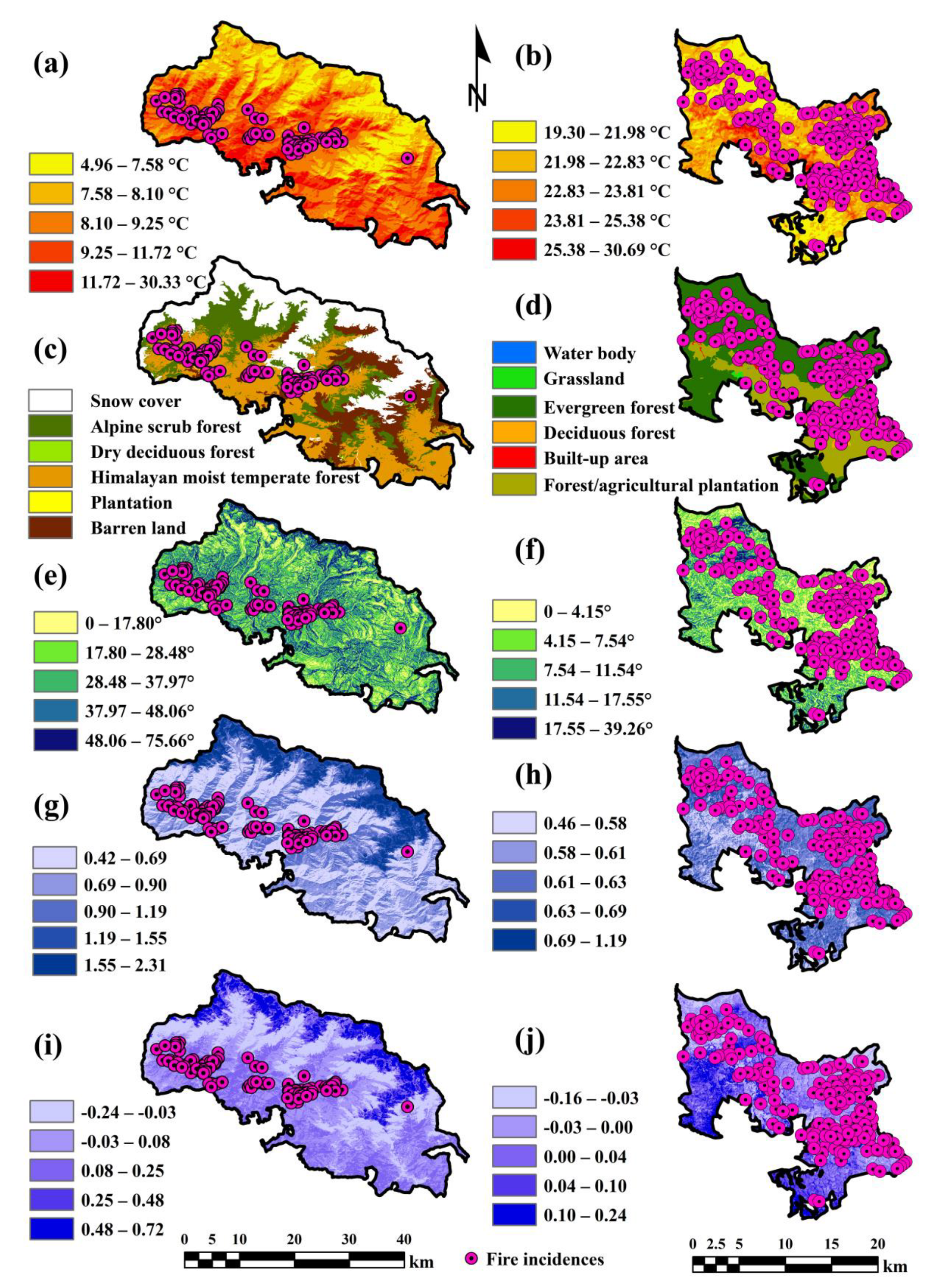
3.3. Conditioning Factors

The conditioning factors that are responsible for the initiation of fires were selected based on the previous studies [22,24,36,119], and the concept of Chuvieco et al. [21], which states fire risk as the likelihood that a fire would initiate.

3.3.1. LST

The LST was anticipated to have a crucial relationship with wildfires because the temperature is a major determinant of the fuel moisture content that is linked to fire ignition, spread, and behavior. The study by Manzo-Delgado et al. [120] found the LST as an integral factor contributing to the vulnerability of vegetation and is a crucial factor to be included in wildfire risk modeling. The LST of KWLS was classified into five classes and ranges from 4.96 to 30.33 °C (Figure 4a). The lower LST was confined to the northern and northeastern portions of the KWLS covered by snow cover. It was observed that a total of 90 fires (72.58%) occurred in areas with a higher LST (11.72–30.33 °C), followed by 22 fires (17.74%) in areas with an LST value range of 9.25–11.72 °C. The LST of the WWLS ranged from 19.30 to 30.69 °C (Figure 4b) and was categorized into five classes. It was observed that a total of 8 fires (4.16%) occurred in areas with the highest LST (25.38–30.69 °C), followed by 20 fires (10.41%) in areas with the lowest LST value range of 23.81–25.38 °C.

Since the temperature range is different for the two study areas, the influence of the temperature on wildfire initiation was assessed by verifying the LST value of each fire point. It is observed that the majority of fires (53 fires, or 42.74%) occurred in areas with temperatures ranging from 12.0 °C to 16.0 °C for the KWLS. Similarly for the WWLS, it is observed that the majority of fires (90 fires, or 72.58%) occurred in areas with temperatures ranging from 22.7 °C to 23.7 °C. This reiterates that the LST does not have a significant influence on fire initiation in both the KWLS and the WWLS.

3.3.2. Land Cover Types

Vegetation acts as a fuel for wildfires, whereas its type and structure (spacing) determine the spread and intensity of wildfires [22]. Areas with dry and thick vegetation are more prone to fires, as fires can spread easily [121]. The plantation areas are also prone to fires, as the areas are non-forested and are managed by people; hence, there is a chance of accidental fires. Fires are also set by the farmers to clear the dried and fallen leaves and barks and to promote the growth of grass and fodder [5]. Gómez-González et al. [122] also found that undermanaged forest plantations can pose a threat to human populations by causing wildfires. The land cover types present in the KWLS include snow cover, Alpine scrub forest, dry deciduous forest, Himalayan moist temperate forest, plantations, and barren land (Figure 4c). The north, northeast, and northwest parts of the sanctuary are covered by snow and, hence, are devoid of fire. A total of 57 fires (45.96%) occurred in the Alpine scrub forest, and 57 fires (45.96%) occurred in the Himalayan moist temperate forest. The land cover types present in the WWLS include water bodies, grassland, forest/agricultural plantations, evergreen forest, deciduous forest, and built-up areas (Figure 4d). There were 107 fires (55.73%) in evergreen forests and 73 fires (38.02%) in forest/agricultural plantations.

3.3.3. Slope

The slope of the terrain accelerates the spread of fire [123]. The steeper the slope, the faster a fire can move, as it preheats and pre-dries the terrain above it [124,125]. The slope of the KWLS ranges between 0 and 75.66° (Figure 4e). A total of 11 fire incidences (8.87%) were observed in areas with a slope ranging from 48.06° to 75.66°. 51 fires (41.13%) occurred in areas with a slope range of 37.97–48.06° and 38 fires (30.64%) occurred in areas with a slope range of 28.48–37.97°. This reiterates that slope has a considerable influence on fire spread and initiation in the KWLS. However, the slope of the WWLS ranges between 0 and 39.26° (Figure 4f). A total of 4 fire incidences (2.08%) were observed in areas with a slope ranging from 17.55 to 39.26 °; 13 fires (6.77%) occurred in areas with a slope range of 11.54–17.55 °; and 38 fires (19.79%) occurred in areas with a slope range of 7.54–11.54°. The WWLS forms a part of the Wayanad Plateau, an extension of the Mysore plateau, and is hence characterized by a low slope. Thus, the slope has less control over the spread of forest fires.

3.3.4. WRI

AWRI score above one represents a water body [82], and, hence, the probability of fire occurrence is higher in areas with lower WRI values. In the case of the KWLS, higher WRI values were observed in the areas covered by snow. The WRI of the KWLS ranges between 0.42 and 2.31 (Figure 4g). A total of 102 fire incidences (82.25%) have been recorded in areas with lower WRI values (0.42–0.69), reiterating the influence of soil moisture on fire spread in the KWLS. The WRI of the WWLS ranges between 0.46 and 1.19 (Figure 4h). In the case of the WWLS, a total of 16 fire incidences (8.33%) have been recorded in areas with a WRI value range of 0.42–0.69, followed by 50 fires (26.04%) in areas with a WRI range of 0.58–0.61. This demonstrates that the WRI has only a considerable influence on fire spread and initiation in the WWLS.

3.3.5. NDWI

The NDWI is used to assess the moisture level in plants and the surrounding soil and ranges between −1 and +1 [24]. The chance of fire is high in the areas with lower NDWI values (moisture) [24]. The NDWI of the KWLS ranges from −0.24 to 0.72 and was categorized into five classes (Figure 4i). Higher NDWI values are confined to the north and northeast areas covered by snow cover in the KWLS. In this sanctuary, the areas with lower–moderate NDWI values have a higher number of fire incidences: 63 fires (50.80%) in areas with an NDWI value range of −0.03–0.08, followed by 57 fires (45.96%) in areas with an NDWI value range of 0.08–0.25. Whereas the NDWI of the WWLS ranges from −0.16 to 0.24 and was categorized into five classes (Figure 4j). In the WWLS, the areas with lower–moderate NDWI values have a higher number of fire incidences. A total of 41 fires (21.35%) were reported in areas with an NDWI value range between −0.16 and −0.03, followed by 81 fires (42.18%) in areas with an NDWI value range of −0.03–0.00, and 44 fires (22.1%) were reported in areas with an NDWI value range of 0.00–0.04. This underlines that the NDWI has a significant influence on fire spread in the KWLS but only a considerable influence in the WWLS.

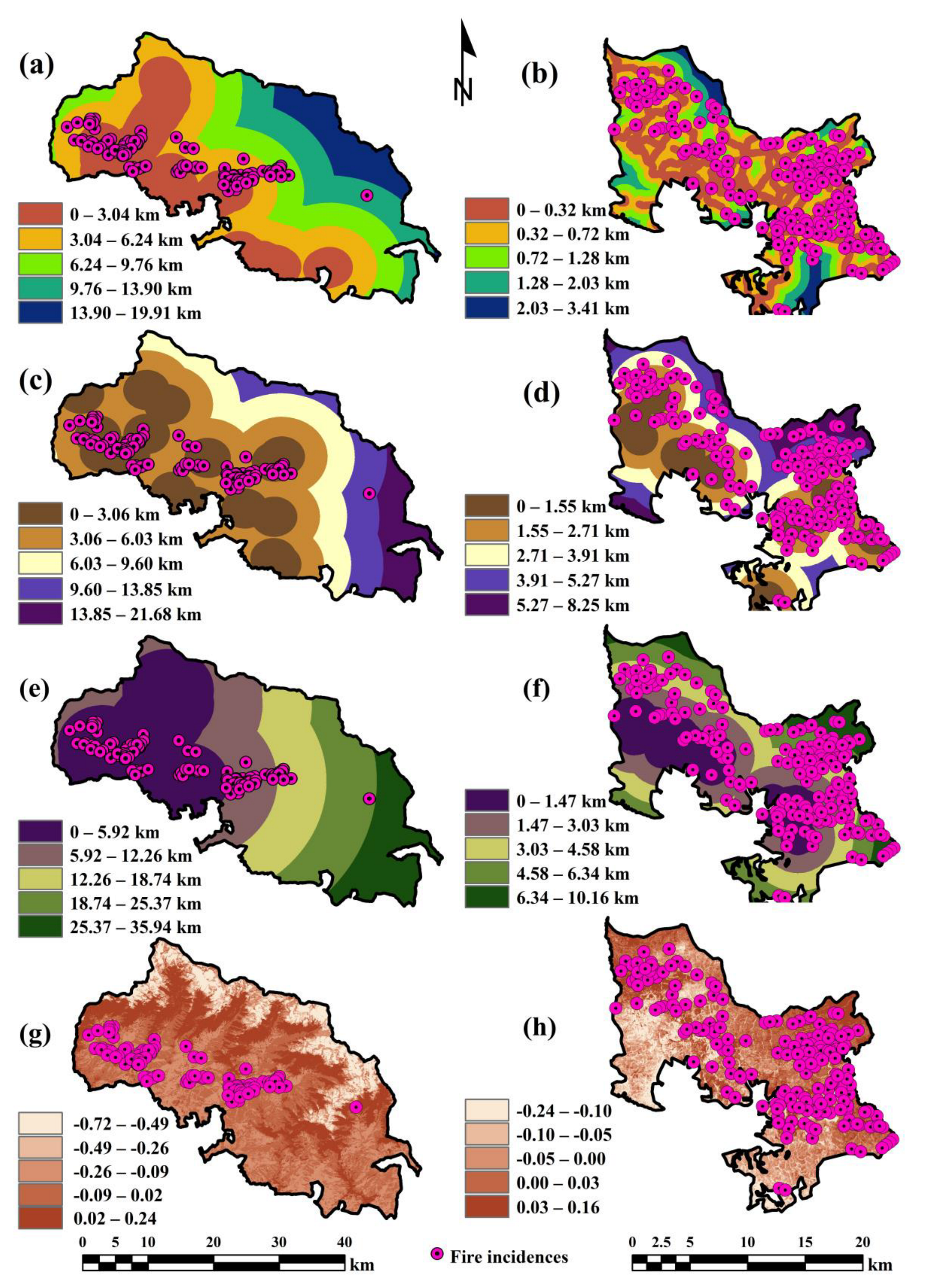
3.3.6. Distance from the Road

The KWLS and WWLS are popular tourist spots, and, hence, a lot of tourists visit every year. The passage of tourists and pilgrims through these forest roads can cause wildfires from fires set to clear forest paths, extinguish cigarettes, cook, create campfires, and to construct and repair roads through coal tar burning [5,22,126]. The risk of wildfires is, therefore, higher in places that are located near road networks. In the KWLS, the road networks are confined to the south, southeast, southwest, and northwest parts of the sanctuary. Based on the distance from the road, the sanctuary area has been categorized into five zones: 0–3.04 km; 3.04–6.24 km; 6.24–9.76 km; 9.76–13.90 km; and 13.90–19.91 km (Figure 5a). In total, 77 fires (62.09%) occurred in areas closer to the road (0–3.04 km). The WWLS has a good road network. Based on the distance from the road, the sanctuary area has been categorized into five zones (0–0.32 km; 0.32–0.72 km; 0.72–1.28 km; 1.28–2.03 km; and 2.03–3.41 km) (Figure 5b). In total, 94 fires (48.95%) were recorded in areas closer to the road (0–0.32 km). This shows that road networks have a significant influence on the KWLS and WWLS.

3.3.7. Distance from the Tourist Spot, and Pilgrim/Religious Center

Tourist spots and pilgrim/religious centers are sites of mass gatherings. The number of pilgrim/religious centers is higher in the KWLS compared to the WWLS. Both sanctuaries are home to many famous tourist spots. Hence, the areas closer to tourist spots and pilgrim/religious centers are more prone to wildfires, as the fires created for recreational activities and religious rituals can escalate into wildfires due to carelessness [5]. There are many tourist spots and pilgrim/religious centers in the KWLS, except in the north, east, northeast, and southeast parts. Based on the distance from the tourist spot and pilgrim/religious center, the KWLS is categorized into five zones: 0–3.06 km, 3.06–6.03 km, 6.03–9.60 km, 9.60–13.85 km, and 13.85–21.68 km (Figure 5c). A total of 92 fires (74.19%) occurred in areas closer to tourist spots and pilgrim/religious centers (0–3.06 km). Similar to the KWLS, the WWLS also has many tourist spots. Based on the distance from the tourist spot and pilgrim/religious center, the WWLS is categorized into five zones: 0–1.55 km; 1.55–2.71 km; 2.71–3.91 km; 3.91–5.27 km; and 5.27–8.25 km (Figure 5d). A total of 53 fires (27.60%) occurred in areas closer to tourist spots and pilgrim/religious centers (0–1.55 km). This confirms its higher influence in the KWLS and its lesser influence in the WWLS.

3.3.8. Distance from the Settlement

The local populace residing in the sanctuaries can light fires as a part of their traditions and religious customs, to burn agricultural wastes, drive away wild animals, clear paths, collect forest products, extract wine, make charcoal, for resin tapping, setting campfires, cooking, and by throwing unextinguished cigarettes [5]. Furthermore, poachers or smugglers can create wildfires by the fires set to hide illicit felling of trees, encroach on forest land, or as a result of personal rivalries [5]. Thus, wildfires are more likely to break out in areas of human settlement [24]. In the KWLS, the human settlements are confined to the west, northwest, and southwest parts. Based on the distance from the settlement, the Kedarnath Wildlife Sanctuary was categorized into five zones: 0–5.92 km, 5.92–12.26 km, 12.26–18.74 km, 18.74–25.37 km, and 25.37–35.94 km (Figure 5e). A total of 77 fire incidences (62.09%) have been observed in areas closer to human settlements (0–5.92 km). On the other hand, the WWLS has a large number of human settlements, especially in the western and southeastern parts of the sanctuary. Based on the distance from the settlement, the WWLS was categorized into five zones: 0–1.47 km; 1.47–3.03 km; 3.03–4.58 km; 4.58–6.34 km; and 6.34–10.16 km (Figure 5f). A total of 51 fire incidences (26.56%) have been observed in areas closer to human settlements (0–1.47 km). The above observations confirm that human settlements have a higher influence in the KWLS than in the WWLS.

3.3.9. NDBI

The NDBI was employed to extract built-up areas, and the value ranged between −1 and +1 [83]. The negative NDBI values represent a water body or areas with higher soil moisture content; the higher positive NDBI values represent built-up areas, and the lower positive NDBI values represent vegetation. Consequently, the probability of fire will be high in regions with lower positive NDBI values. The NDBI of the KWLS ranges from −0.72 to 0.24 (Figure 5g) and was categorized into five classes. A total of 72 fires (58.06%) were recorded in areas with the NDBI values ranging from −0.09 to 0.02. The NDBI of the WWLS ranges from −0.24 to 0.16 (Figure 5h) and was categorized into five classes. A total of 82 fires (42.70%) were recorded in areas with the NDBI values ranging from 0.00 to 0.03. This confirmed that the NDBI has a significant influence on fire spread in both the KWLS and the WWLS.

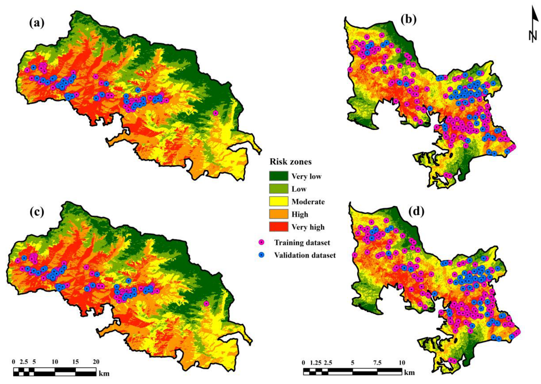
3.4. Wildfire Risk Zones

This study established beyond doubt that land cover types, WRI, distance from the tourist spot and pilgrim/religious center, distance from the road, distance from the settlement, NDBI, and slope all have a significant impact on fire spread in the KWLS. This reiterates the fact that fire occurrence in this sanctuary is due to natural as well as human-induced (anthropogenic) factors. Similarly, this study also confirmed that distance from the road, land cover types, NDWI, WRI, distance from the settlement, and distance from tourist spots and pilgrim/religious centers all have a significant impact on fire initiation and spread in the WWLS. However, the slope and the LST do not have a substantial impact on fire spread in the WWLS. Anthropogenic factors are predominant in the occurrence and spread of fire in the WWLS. Figure 6a,b depict the wildfire risk zones in the KWLS and the WWLS employing the AHP models, and Figure 6c,d depict the wildfire risk zones in the KWLS and the WWLS employing the F-AHP models, respectively. The percentage of each risk zone is shown in

Table 9. Percentage of fire risk zones in KWLS and WWLS.

Risk Zones	Percentage of Risk Zones in KWLS		Percentage of Risk Zones in WWLS
	AHP Model	F-AHP Model	AHP Model	F-AHP Model
Very low	16.59	16.59	8.43	8.45
Low	16.70	16.54	17.92	17.70
Moderate	16.92	17.50	27.62	27.75
High	26.61	26.88	29.08	28.98
Very high	23.18	22.49	16.95	17.12
Total	100	100	100	100

.

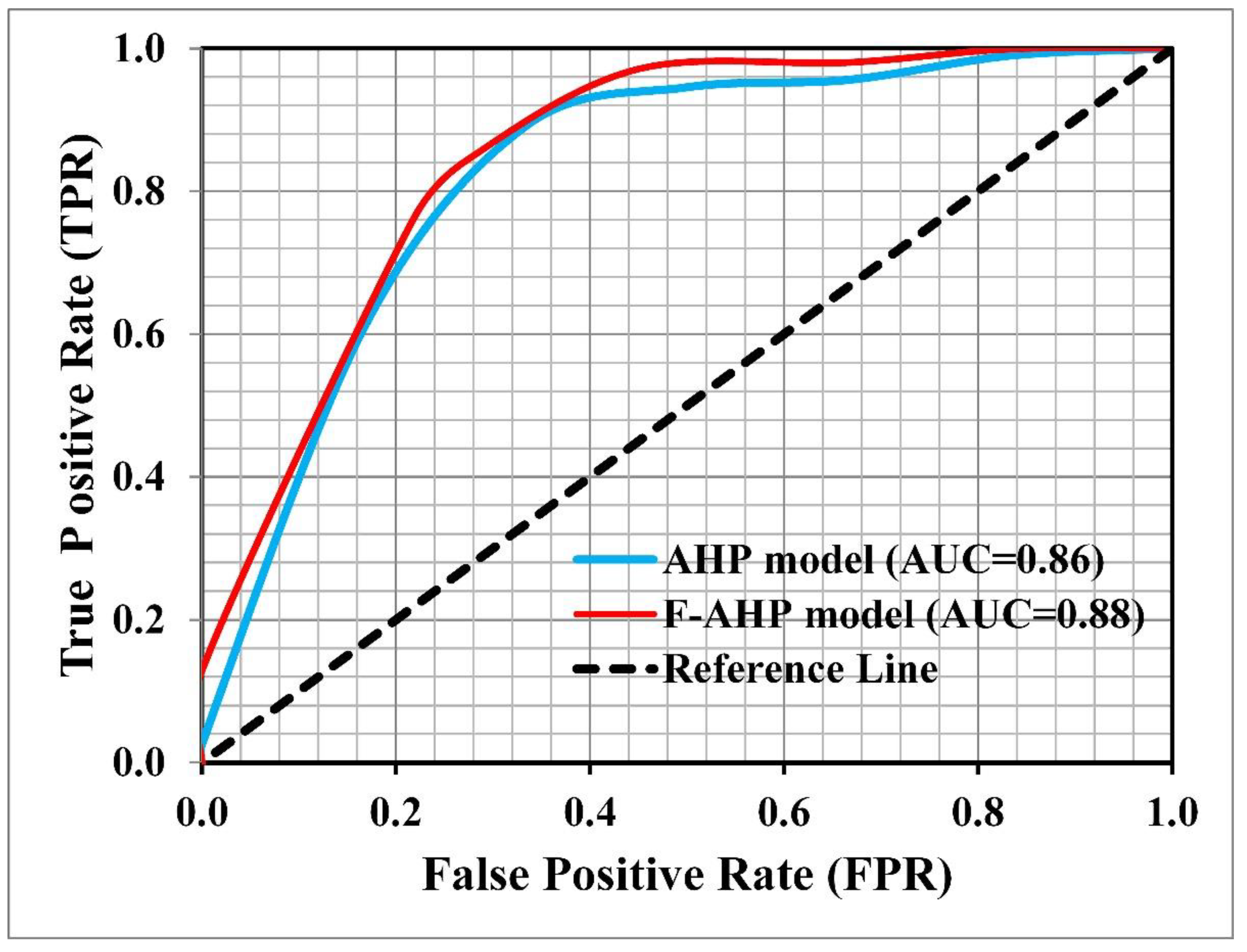
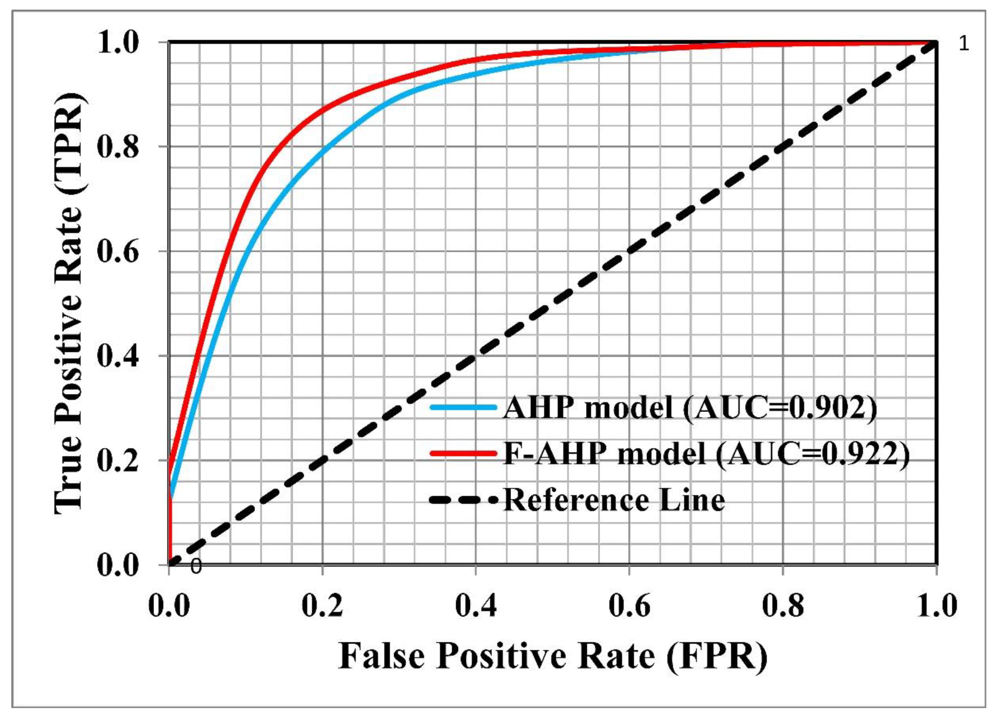
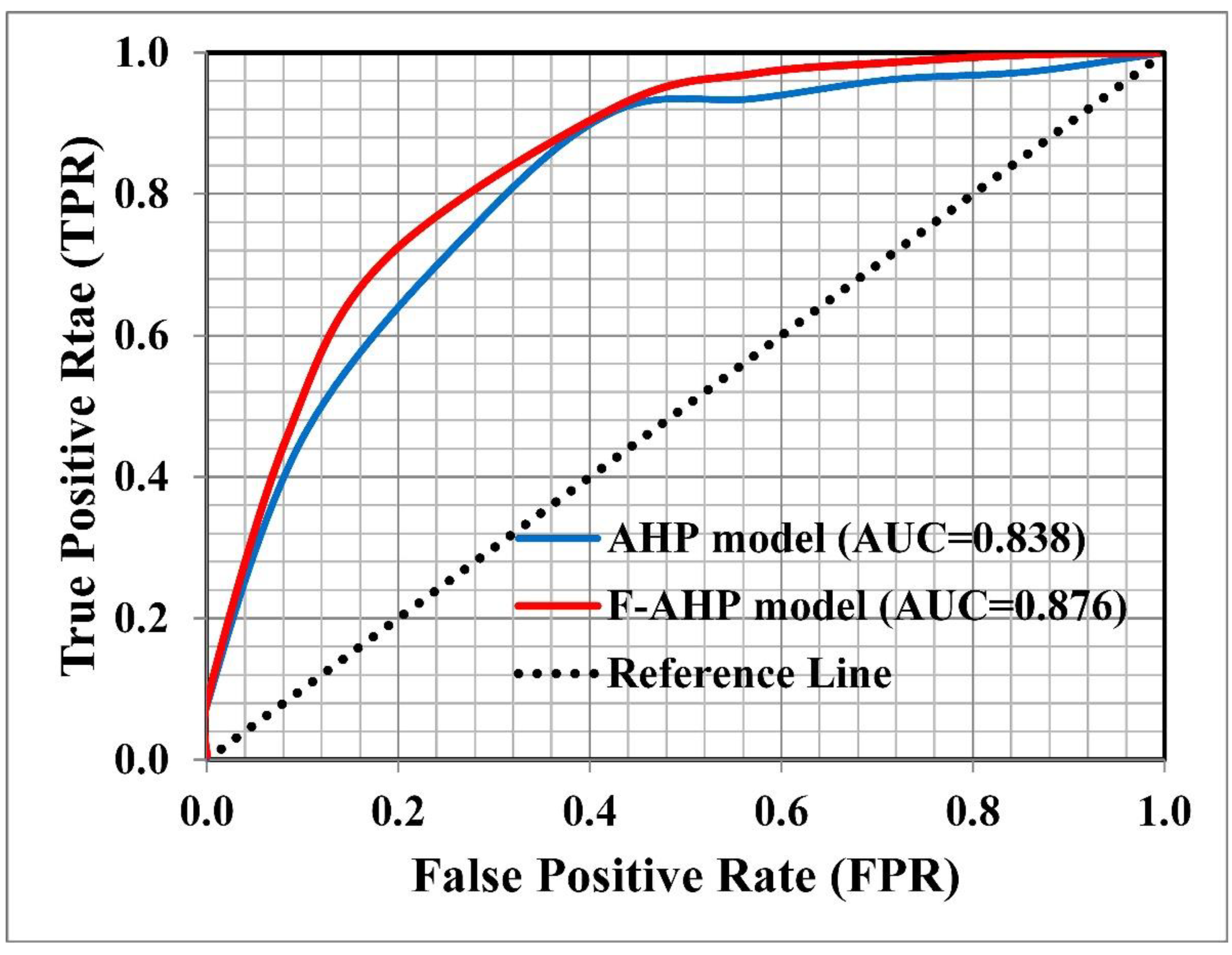
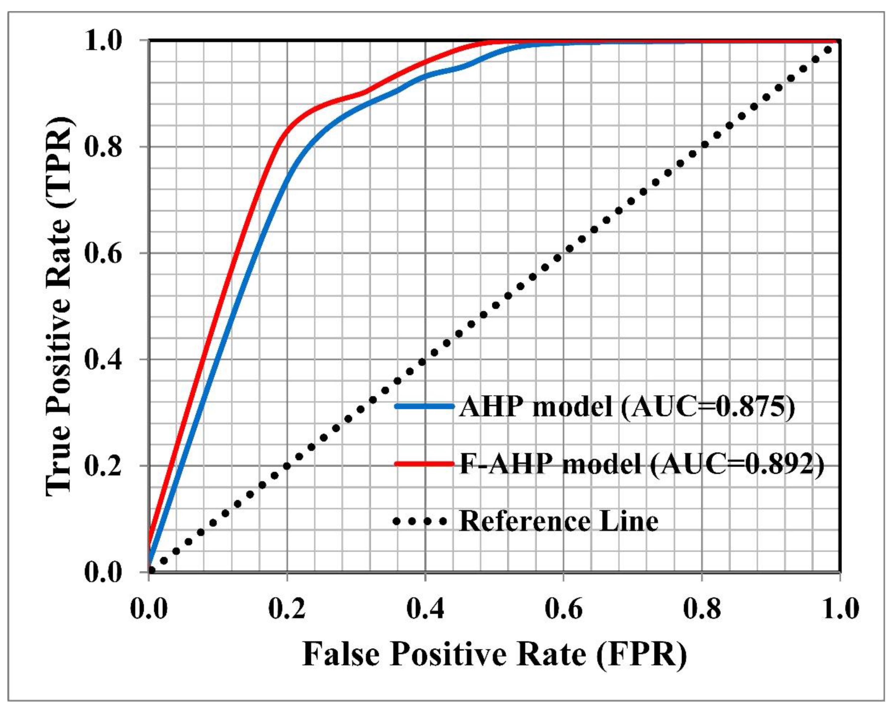
3.5. Validation of the Risk Zone Maps

For the KWLS, the ROC curve analysis of the training dataset provided good AUC values of 0.860 (86.0%) and 0.880 (88.0%) for the AHP and F-AHP models, respectively (Figure 7), and the validation dataset provided excellent AUC values of 0.902 (90.2%) and 0.922 (92.2%), respectively (Figure 8). For the WWLS, the ROC curve analysis of the training dataset provided good AUC values of 0.838 (83.8%) and 0.876 (87.6%) for the AHP and F-AHP models, respectively (Figure 9), and the validation dataset provided good AUC values of 0.875 (87.5%) and 0.892 (89.2%), respectively (Figure 10). Thus, it was proven beyond doubt that both models are very effective in mapping wildfire risk zones, with the F-AHP model having slightly better accuracy than the AHP model.

For the validation dataset of the KWLS, the matrices such as sensitivity, accuracy, and Kappa index confirmed higher scores of 0.714, 0.737, and 0.870 for the AHP model and 0.810, 0.842, and 0.884 for the F-AHP model, respectively (

Table 10. Validation matrices—KWLS.

Matrices	Training Dataset		Validation Dataset
	AHP	F-AHP	AHP	F-AHP
Sensitivity	0.714	0.771	0.714	0.810
Accuracy	0.742	0.806	0.737	0.842
Kappa index	0.840	0.850	0.870	0.884

). For the validation dataset of the WWLS, the matrices such as sensitivity, accuracy, and Kappa index confirmed higher scores of 0.846, 0.875, and 0.850 for the AHP model and 0.905, 0.926, and 0.875 for the F-AHP model, respectively (

Table 11. Validation matrices—WWLS.

Matrices	Training Dataset		Validation Dataset
	AHP	F-AHP	AHP	F-AHP
Sensitivity	0.800	0.840	0.846	0.905
Accuracy	0.813	0.845	0.875	0.926
Kappa index	0.762	0.829	0.850	0.875

). The Kappa scores of the classification indicate perfect agreement for both models.

4. Discussion

The two wildlife sanctuaries, the KWLS and the WWLS, experiencing different climatic conditions, were selected for wildfire mapping to showcase how the influencing factors differ, with a special focus on the distinction between natural and anthropogenic factors. Furthermore, this study also attempted to show how the wildfire zones differ in such contrasting climatic conditions. While a sub-tropical humid climate with hot and humid summers and cool winters is characteristic of the KWLS, the WWLS experiences a tropical monsoon climate. With the dawn of climate change and subsequent increases in temperature, one of the most pronounced catastrophes is forest fires. A literature review of different natural hazards reveals that one of the least studied hazards is forest fires, but it is the one that causes severe destruction to natural resources as well as deteriorates the atmosphere with the emission of smoke for several days. Thus, it is quintessential to study and prioritize the factors that facilitate forest fires. Furthermore, the boom in the tourism industry and the expansion of agriculture into the forest regions also warrant a study of the interplay of anthropogenic factors and natural factors. Moreover, both areas of study require the identification of factors that are responsible for forest fires, as these two areas have several unique features. The KWLS forms one of the major pilgrimages in the Indian subcontinent. Hindu temples such as Rudranath, Tungnath, Madhyamaheshwar, and Triyuginarayan are within this sanctuary. The famous Kedarnath temple is located just outside its northern border. However, the entire Gaurikund-Kedarnath route is within this sanctuary. Many pilgrims visit these temples every year. Apart from several national parks within its vicinity, such as Nagarhole, Bandipur, and Mudumalai, a large number of tribal populations live within the WWLS.

This study identified both natural and anthropogenic factors responsible for forest fires. The natural factors in both the study areas include factors such as the natural land cover as well as derivatives such as the WRI and the NDWI, whereas the anthropogenic factors include distance from the pilgrim and tourist centers, distance from the road, and distance from the settlement, as well as derivatives such as the NDBI. In the KWLS, the majority of fires occurred in the Alpine scrub forest and Himalayan moist temperate forest, whereas in the WWLS, most fire occurrences were recorded in the evergreen forest, followed by the plantation areas. Though the biodiversity of temperate forests is much lower than that of tropical forests, they host the largest and oldest species [127]. The moderate weather, fertile soils, and lush vegetation of temperate forests have made them ideal for human settlement, agricultural development, and the direct use of trees for fuel and timber [127,128]. The anthropogenic activities such as widespread crop cultivation, livestock grazing, the gathering of mulch, and alteration of natural water drainage [128] in these types of forests make them more vulnerable to fires. The Alpine scrub forest comprises shrubs, grasses, and short trees such as junipers, pines, and birches, and extends up to areas just below the snowline. These types of vegetation are also prone to wildfires. Nikhil et al. [22] reported higher fire incidences in evergreen forests. Moisture-related factors such as the NDWI and the WRI show significant influence in the KWLS and only considerable influence in the WWLS. The lower influence of moisture-related factors in the WWLS maybe since the correlation depends on land cover heterogeneity and soil type [129]. The study by Nikhil et al. [22] also ascertained the fact that moisture has a significant influence on fire spread as it determines the ignition probability and behaviour of fire [130]. However, the LST does not show a significant influence on fire spread in the KWLS and the WWLS. However, according to Parajuli et al. [131], one of the reasons for fire propagation in two major landscapes in Nepal is due to the higher LST (temperature between 30 and 35 °C). Though the slope has a considerable influence in the KWLS but not in the WWLS, this could be due to the plateau-like topography seen in the WWLS.

While considering the anthropogenic factors, apart from the land cover, which was described earlier, the NDBI has a significant influence on the KWLS and a considerable impact on the WWLS. The probability of fire is low in areas with negative as well as higher positive NDBI values, as these are zones with little or no vegetation (fuel). Other anthropogenic factors such as distance from the tourist spots, pilgrim/religious center, roads, and settlements show significant influence in the KWLS, whereas, in the case of the WWLS, only the road shows a significant influence. The WWLS has a large number of road networks, and 94 fires (48.95%) occurred in the vicinity of roads. Anthropogenic factors such as proximity to roads and settlements were employed by Ajin et al. [132,133] and Nikhil et al. [22]; they found higher fire incidences in areas closer to roads and human settlements. Such anthropogenic activities have created a higher number of fire incidences even in the evergreen forest. Similarly, the higher influence of anthropogenic factors in the WWLS manifested as the reason for higher fire incidences in the areas of lower LST.

The efficacy of the wildfire risk zone map created employing the AHP model has been proven by researchers such as Amrutha et al. [36], Nikhil et al. [22], and Pradeep et al. [24] with an AUC value above 0.70, which depicts fair prediction capability. While comparing AHP and frequency ratio (FR) models, Pradeep et al. [24] found AHP as the ideal model for wildfire risk zone mapping of Eravikulam National Park in South India, with an AUC value of 0.767, in comparison to the FR model with a failure AUC value of 0.567. While comparing the AHP and F-AHP models, researchers such as Abdi et al. [54], Akshaya et al. [53], Bouamrane et al. [55], and Vilasan and Kapse [56] found that F-AHP has better prediction capability than the AHP model. The research by Tiwari et al. [52] also found that the F-AHP (0.83) model has better prediction accuracy than the AHP (AUC: 0.81) and FR (AUC: 0.77) models when comparing these three models for demarcating forest fire susceptible areas in Pauri Garhwal in North India. This justified the selection of the AHP and F-AHP models for this research.

An integral part of risk or susceptibility modelling is the validation of created maps [45]. An ROC curve is an efficient method for assessing the accuracy of maps [119,134]. For the training dataset, the AUC value of the F-AHP model confirmed a 2.00% increase over the AHP model for the KWLS and a 3.80% increase for the WWLS. For the validation dataset, the AUC value of the F-AHP model confirmed a 2.00% increase over the AHP model for the KWLS. Whereas for the WWLS, the AUC value of the F-AHP model confirmed a 1.70% increase over the AHP model. For the validation dataset of the KWLS, the sensitivity, accuracy, and Kappa index values of the F-AHP models confirmed a slight increase of 0.096 (from 0.714 to 0.810), 0.105 (from 0.737 to 0.842), and 0.014 (from 0.870 to 0.884) over the AHP model, whereas for the WWLS (validation dataset), the sensitivity, accuracy, and Kappa index values of the F-AHP model again confirmed a slight increase of 0.059 (from 0.846 to 0.905), 0.051 (from 0.875 to 0.926), and 0.025 (from 0.850 to 0.875)over the AHP model. The perfect agreement in Kappa scores and higher AUC, sensitivity, and accuracy values confirmed F-AHP as the better model than the AHP model. The validation matrices such as sensitivity, accuracy, and the Kappa index have been employed by many researchers [135,136] for assessing the performance of maps.

The result of this modelling can be improved by integrating factors such as wind speed and relative humidity. Though the wind speed data can be acquired from the Global Wind Atlas data portal (https://globalwindatlas.info/ (accessed on 20 July 2022)), the coarse spatial resolution of 250 m and its downscaled nature prevented us from using it in this analysis. The relative humidity data can be acquired from the NCEP reanalysis grid (https://psl.noaa.gov/data/gridded/data.ncep.reanalysis2.html (accessed on 20 July 2022)), but the spatial resolution was very poor (25° or ~250 km), making it not suitable for smaller areas. However, Achu et al. [137] combined climatic data for modelling the wildfire susceptibility of the Wayanad district, which entirely covered the WWLS, covering an area of 2130 km², where a downscaled 250 m resolution dataset would be ideal. However, the present study demonstrated a better AUC value than the study of Achu et al. [137]. Additionally, the study by Tiwari et al. [52] conducted in a district in the Uttarakhand state of India, with similar climatic conditions to those of the KWLS, has a lower performance (AUC value: 0.83) than that of this study. The better validation scores of the results of this study ascertained the fact that the factors and models selected are highly relevant.

5. Conclusions

Wildfires are one of the most common and frequently occurring catastrophes that pose threats to protected areas, such as wildlife sanctuaries in India, and have resulted in an enormous loss of rich flora and fauna. These protected areas are home to many rare and endangered species. Consequently, the implementation of appropriate mitigation measures is very necessary. This study demarcated the wildfire risk zones in two protected areas in India using satellite data and geospatial techniques. This study established beyond a hint of doubt that factors including the land cover types, WRI, distance from tourist spots and pilgrim/religious centers, distance from the road, distance from the settlement, NDBI, and slope have a substantial impact on fire spread in the KWLS. Similarly, this modelling proved that factors including the distance from the road, land cover types, NDWI, WRI, distance from the settlement, and distance from tourist spots and pilgrim/religious centers have a substantial impact on fire spread in the WWLS. The influence of anthropogenic factors was high in both the WWLS and the KWLS. This was due to the high number of roads in the WWLS and the presence of many pilgrim centers (temples) in the KWLS. Thus, this study also reiterates the greater influence of anthropogenic factors. The AUC values for the AHP and F-AHP models proved that both models are effective (with good and excellent values) in demarcating wildfire risk zones. However, the F-AHP was found to be more efficient than the AHP model. The validation matrices such as sensitivity, accuracy, and Kappa index also confirmed better scores for the F-AHP model. As a result, the F-AHP model was chosen as the ideal model, and 22.49% of the KWLS and 17.12% of the WWLS fall within the very-high-risk zones according to the F-AHP model. The created maps will aid officials working with forest and disaster management departments in selecting appropriate measures to mitigate wildfires in critical areas.

References

1. Reddy, C.S.; Bird, N.G.; Sreelakshmi, S.; Manikandan, T.M.; Asra, M.; Krishna, P.H.; Jha, C.S.; Rao, P.V.N.; Diwakar, P.G. Identification and characterization of spatio-temporal hotspots of forest fires in South Asia. Environ. Monit. Assess. 2019, 191, 791. [Google Scholar] [CrossRef] [PubMed]
2. Yadav, I.C.; Devi, N.L. Biomass burning, regional air quality, and climate change. In Encyclopedia of Environmental Health, 2nd ed.; Nriagu, J., Ed.; Elsevier: Amsterdam, The Netherlands, 2019; pp. 386–391. [Google Scholar] [CrossRef]
3. Cai, Y.F.; Zhang, H.; Feng, Z.; Shen, S.Z. Intensive Wildfire Associated With Volcanism Promoted the Vegetation Changeover in Southwest China During the Permian−Triassic Transition. Front. Earth Sci. 2021, 9, 615841. [Google Scholar] [CrossRef]
4. Zhao, H.; Li, X.; Hall, V.A. Holocene vegetation change in relation to fire and volcanic events in Jilin, Northeastern China. Sci. China Earth Sci. 2015, 58, 1404–1419. [Google Scholar] [CrossRef]
5. Satendra; Kaushik, A.D. Forest Fire Disaster Management; National Institute of Disaster Management, Ministry of Home Affairs: New Delhi, India, 2014.
6. Morgan, J.; Artemieva, N.; Goldin, T. Revisiting wildfires at the K-Pg boundary. J. Geophys. Res. Biogeosci. 2013, 118, 1508–1520. [Google Scholar] [CrossRef]
7. Tedim, F.; Xanthopoulos, G.; Leone, V. Forest fires in Europe: Facts and challenges. In Wildfire Hazards, Risks and Disasters; Shroder, J.F., Paton, D., Eds.; Elsevier: Amsterdam, The Netherlands, 2015; pp. 77–99. [Google Scholar] [CrossRef]
8. Xu, R.; Yu, P.; Abramson, M.J.; Johnston, F.H.; Samet, J.M.; Bell, M.L.; Haines, A.; Ebi, K.L.; Li, S.; Guo, Y. Wildfires, global climate change, and human health. N. Engl. J. Med. 2020, 383, 2173–2181. [Google Scholar] [CrossRef]
9. Wang, B.; Luo, X.; Yang, Y.M.; Liu, J. Historical change of El Niño properties sheds light on future changes of extreme El Niño. Proc. Natl. Acad. Sci. USA 2019, 116, 22512–22517. [Google Scholar] [CrossRef] [Green Version]
10. Zeng, Z.; Ziegler, A.D.; Searchinger, T.; Yang, L.; Chen, A.; Ju, K.; Piao, S.; Li, L.Z.X.; Ciais, P.; Chen, D.; et al. A reversal in global terrestrial stilling and its implications for wind energy production. Nat. Clim. Chang. 2019, 9, 979–985. [Google Scholar] [CrossRef]
11. Karnauskas, K.B.; Lundquist, J.K.; Zhang, L. Southward shift of the global wind energy resource under high carbon dioxide emissions. Nat. Geosci. 2018, 11, 38–43. [Google Scholar] [CrossRef]
12. Bowman, D.M.J.S.; Kolden, C.A.; Abatzoglou, J.T.; Johnston, F.H.; van der Werf, G.R.; Flannigan, M. Vegetation fires in the Anthropocene. Nat. Rev. Earth Environ. 2020, 1, 500–515. [Google Scholar] [CrossRef]
13. Hurteau, M.D.; Liang, S.; Westerling, A.L.; Wiedinmyer, C. Vegetation-fire feedback reduces projected area burned under climate change. Sci. Rep. 2019, 9, 2838. [Google Scholar] [CrossRef] [Green Version]
14. Sun, Q.; Miao, C.; Hanel, M.; Borthwick, A.G.L.; Duan, Q.; Ji, D.; Li, H. Global heat stress on health, wildfires, and agricultural crops under different levels of climate warming. Environ. Int. 2019, 128, 125–136. [Google Scholar] [CrossRef] [PubMed]
15. Turco, M.; Rosa-Cánovas, J.J.; Bedia, J.; Jerez, S.; Montávez, J.P.; Llasat, M.C.; Provenzale, A. Exacerbated fires in Mediterranean Europe due to anthropogenic warming projected with non-stationary climate-fire models. Nat. Commun. 2018, 9, 3821. [Google Scholar] [CrossRef] [PubMed] [Green Version]
16. Cieslik, S.; Tuovinen, J.P.; Baumgarten, M.; Matyssek, R.; Brito, P.; Wieser, G. Gaseous exchange between forests and the atmosphere. In Developments in Environmental Science; Matyssek, R., Clarke, N., Cudlin, P., Mikkelsen, T.N., Tuovinen, J.P., Wieser, G., Paoletti, E., Eds.; Elsevier: Amsterdam, The Netherlands, 2013; Volume 13, pp. 19–36. [Google Scholar] [CrossRef]
17. Harper, A.R.; Doerr, S.H.; Santin, C.; Froyd, C.A.; Sinnadurai, P. Prescribed fire and its impacts on ecosystem services in the UK. Sci. Total Environ. 2018, 624, 691–703. [Google Scholar] [CrossRef] [PubMed] [Green Version]
18. Junaidi, S.N.; Khalid, N.; Othman, A.N.; Hamid, J.R.A.; Saad, N.M. Analysis of the relationship between forest fire and land surface temperature using Landsat 8 OLI/TIRS imagery. IOP Conf. Ser. Earth Environ. Sci. 2005, 767, 012005. [Google Scholar] [CrossRef]
19. Liu, Z.; Ballantyne, A.P.; Cooper, L.A. Biophysical feedback of global forest fires on surface temperature. Nat. Commun. 2019, 10, 214. [Google Scholar] [CrossRef] [Green Version]
20. Vlassova, L.; Pérez-Cabello, F.; Mimbrero, M.R.; Llovería, R.M.; García-Martín, A. Analysis of the relationship between land surface temperature and wildfire severity in a series of Landsat images. Remote Sens. 2014, 6, 6136–6162. [Google Scholar] [CrossRef] [Green Version]
21. Chuvieco, E.; Aguado, I.; Jurdao, S.; Pettinari, M.L.; Yebra, M.; Salas, J.; Hantson, S.; de la Riva, J.; Ibarra, P.; Rodrigues, M.; et al. Integrating geospatial information into fire risk assessment. Int. J. Wildland Fire 2014, 23, 606–619. [Google Scholar] [CrossRef]
22. Nikhil, S.; Danumah, J.H.; Saha, S.; Prasad, M.K.; Rajaneesh, A.; Mammen, P.C.; Ajin, R.S.; Kuriakose, S.L. Application of GIS and AHP method in forest fire risk zone mapping: A study of the Parambikulam Tiger Reserve, Kerala, India. J. Geovis. Spat. Anal. 2021, 5, 14. [Google Scholar] [CrossRef]
23. Eskandari, S. A new approach for forest fire risk modeling using fuzzy AHP and GIS in Hyrcanian forests of Iran. Arab. J. Geosci. 2017, 10, 190. [Google Scholar] [CrossRef]
24. Pradeep, G.S.; Danumah, J.H.; Nikhil, S.; Prasad, M.K.; Patel, N.; Mammen, P.C.; Rajaneesh, A.; Oniga, V.E.; Ajin, R.S.; Kuriakose, S.L. Forest fire risk zone mapping of Eravikulam National Park in India: A comparison between frequency ratio and analytic hierarchy process methods. Croat. J. For. Eng. 2022, 43, 199–217. [Google Scholar] [CrossRef]
25. Gheshlaghi, H.A.; Feizizadeh, B.; Blaschke, T. GIS-based forest fire risk mapping using the analytical network process and fuzzy logic. J. Environ. Plan. Manage. 2020, 63, 481–499. [Google Scholar] [CrossRef]
26. Jafari Goldarag, Y.; Mohammadzadeh, A.; Ardakani, A.S. Fire risk assessment using neural network and logistic regression. J. Indian Soc. Remote Sens. 2016, 44, 885–894. [Google Scholar] [CrossRef]
27. Shao, Y.; Feng, Z.; Sun, L.; Yang, X.; Li, Y.; Xu, B.; Chen, Y. Mapping China’s forest fire risks with machine learning. Forests 2022, 13, 856. [Google Scholar] [CrossRef]
28. Chen, W.; Zhou, Y.; Zhou, E.; Xiang, Z.; Zhou, W.; Lu, J. Wildfire risk assessment of transmission-line corridors based on naïve bayes network and remote sensing data. Sensors 2021, 21, 634. [Google Scholar] [CrossRef] [PubMed]
29. Janiec, P.; Gadal, S. A comparison of two machine learning classification methods for remote sensing predictive modeling of the forest fire in the North-Eastern Siberia. Remote Sens. 2020, 12, 4157. [Google Scholar] [CrossRef]
30. Song, B.; Kang, S. A method of assigning weights using a ranking and nonhierarchy comparison. Adv. Decis. Sci. 2016, 2016, 8963214. [Google Scholar] [CrossRef] [Green Version]
31. Gavade, R.K. Multi-criteria decision making: An overview of different selection problems and methods. Int. J. Comput. Sci. Inf. Technol. 2014, 5, 5643–5646. [Google Scholar]
32. Olson, D.L. Opportunities and limitations of AHP in multiobjective programming. Math. Comput. Model. 1988, 11, 206–209. [Google Scholar] [CrossRef]
33. Carnero, M.C. Benchmarking of the maintenance service in health care organizations. In Handbook of Research on Data Science for Effective Healthcare Practice and Administration; Noughabi, E., Raahemi, B., Albadvi, A., Far, B., Eds.; IGI Global: Hershey, PA, USA, 2017; pp. 1–25. [Google Scholar] [CrossRef]
34. Abrams, W.; Ghoneim, E.; Shew, R.; LaMaskin, T.; Al-Bloushi, K.; Hussein, S.; AbuBakr, M.; Al-Mulla, E.; Al-Awar, M.; El-Baz, F. Delineation of groundwater potential (GWP) in the northern United Arab Emirates and Oman using geospatial technologies in conjunction with simple additive weight (SAW), analytical hierarchy process (AHP), and probabilistic frequency ratio (PFR) techniques. J. Arid Environ. 2018, 157, 77–96. [Google Scholar] [CrossRef]
35. Kumar, R.; Dwivedi, S.B.; Gaur, S. A comparative study of machine learning and Fuzzy-AHP technique to groundwater potential mapping in the data-scarce region. Comput. Geosci. 2021, 155, 104855. [Google Scholar] [CrossRef]
36. Amrutha, K.; Danumah, J.H.; Nikhil, S.; Saha, S.; Rajaneesh, A.; Mammen, P.C.; Ajin, R.S.; Kuriakose, S.L. Demarcation of forest fire risk zones in Silent Valley National Park and the effectiveness of forest management regime. J. Geovis. Spat. Anal. 2022, 6, 8. [Google Scholar] [CrossRef]
37. Çoban, H.O.; Erdin, C. Forest fire risk assessment using GIS and AHP integration in Bucak forest enterprise, Turkey. Appl. Ecol. Environ. Res. 2020, 18, 1567–1583. [Google Scholar] [CrossRef]
38. Kayet, N.; Chakrabarty, A.; Pathak, K.; Sahoo, S.; Dutta, T.; Hatai, B.K. Comparative analysis of multi-criteria probabilistic FR and AHP models for forest fire risk (FFR) mapping in Melghat Tiger Reserve (MTR) forest. J. For. Res. 2020, 31, 565–579. [Google Scholar] [CrossRef]
39. Kumari, B.; Pandey, A.C. Geo-informatics based multi-criteria decision analysis (MCDA) through analytic hierarchy process (AHP) for forest fire risk mapping in Palamau Tiger Reserve, Jharkhand state, India. J. Earth Syst. Sci. 2020, 129, 204. [Google Scholar] [CrossRef]
40. Lamat, R.; Kumar, M.; Kundu, A.; Lal, D. Forest fire risk mapping using analytical hierarchy process (AHP) and earth observation datasets: A case study in the mountainous terrain of Northeast India. SN Appl. Sci. 2021, 3, 425. [Google Scholar] [CrossRef]
41. Mohammadi, F.; Shabanian, N.; Pourhashemi, M.; Fatehi, P. Risk zone mapping of forest fire using GIS and AHP in a part of Paveh forests. Iran. J. For. Poplar Res. 2011, 18, 569–586. [Google Scholar] [CrossRef]
42. Novo, A.; Fariñas-Álvarez, N.; Martínez-Sánchez, J.; González-Jorge, H.; Fernández-Alonso, J.M.; Lorenzo, H. Mapping forest fire risk—A case study in Galicia (Spain). Remote Sens. 2020, 12, 3705. [Google Scholar] [CrossRef]
43. Nuthammachot, N.; Stratoulias, D. A GIS- and AHP-based approach to map fire risk: A case study of Kuan Kreng peat swamp forest, Thailand. Geocarto Int. 2021, 36, 212–225. [Google Scholar] [CrossRef]
44. Nuthammachot, N.; Stratoulias, D. Multi-criteria decision analysis for forest fire risk assessment by coupling AHP and GIS: Method and case study. Environ. Dev. Sustain. 2021, 23, 17443–17458. [Google Scholar] [CrossRef]
45. Sivrikaya, F.; Küçük, Ö. Modeling forest fire risk based on GIS-based analytical hierarchy process and statistical analysis in Mediterranean region. Ecol. Inform. 2022, 68, 101537. [Google Scholar] [CrossRef]
46. Van Hoang, T.; Chou, T.Y.; Fang, Y.M.; Nguyen, N.T.; Nguyen, Q.H.; Xuan Canh, P.; Ngo Bao Toan, D.; Nguyen, X.L.; Meadows, M.E. Mapping forest fire risk and development of early warning system for NW Vietnam using AHP and MCA/GIS methods. Appl. Sci. 2020, 10, 4348. [Google Scholar] [CrossRef]
47. Eskandari, S.; Miesel, J.R. Comparison of the fuzzy AHP method, the spatial correlation method, and the Dong model to predict the fire high-risk areas in Hyrcanian forests of Iran. Geomat. Nat. Hazards Risk 2017, 8, 933–949. [Google Scholar] [CrossRef] [Green Version]
48. Güngöroğlu, C. Determination of forest fire risk with fuzzy analytic hierarchy process and its mapping with the application of GIS: The case of Turkey/Çakırlar. Hum. Ecol. Risk Assess. 2017, 23, 388–406. [Google Scholar] [CrossRef]
49. Kumi-Boateng, B.; Peprah, M.S.; Larbi, E.K. Prioritization of forest fire hazard risk simulation using hybrid grey relativity analysis (HGRA) and fuzzy analytical hierarchy process (FAHP) coupled with multicriteria decision analysis (MCDA) techniques—A comparative study analysis. Geod. Cartogr. 2021, 47, 147–161. [Google Scholar] [CrossRef]
50. Mehta, D.; Baweja, P.K.; Aggarwal, R.K. Forest fire risk assessment using fuzzy analytic hierarchy process. Curr. World Environ. 2018, 13, 307–316. [Google Scholar] [CrossRef] [Green Version]
51. Sharma, L.K.; Kanga, S.; Nathawat, M.S.; Sinha, S.; Pandey, P.C. Fuzzy AHP for forest fire risk modeling. Disaster Prev. Manage. 2012, 21, 160–171. [Google Scholar] [CrossRef]
52. Tiwari, A.; Shoab, M.; Dixit, A. GIS-based forest fire susceptibility modeling in Pauri Garhwal, India: A comparative assessment of frequency ratio, analytic hierarchy process and fuzzy modeling techniques. Nat. Hazards 2021, 105, 1189–1230. [Google Scholar] [CrossRef]
53. Akshaya, M.; Danumah, J.H.; Saha, S.; Ajin, R.S.; Kuriakose, S.L. Landslide susceptibility zonation of the Western Ghats region in Thiruvananthapuram district (Kerala) using geospatial tools: A comparison of the AHP and Fuzzy-AHP methods. Saf. Extrem. Environ. 2021, 3, 181–202. [Google Scholar] [CrossRef]
54. Abdı, A.; Bouamrane, A.; Karech, T.; Dahri, N.; Kaouachi, A. Landslide susceptibility mapping using GIS-based fuzzy logic and the analytical hierarchical processes approach: A case study in Constantine (North-East Algeria). Geotech. Geol. Eng. 2021, 39, 5675–5691. [Google Scholar] [CrossRef]
55. Bouamrane, A.; Derdous, O.; Dahri, N.; Tachi, S.E.; Boutebba, K.; Bouziane, M.T. A comparison of the analytical hierarchy process and the fuzzy logic approach for flood susceptibility mapping in a semi-arid ungauged basin (Biskra basin: Algeria). Int. J. River Basin Manage. 2022, 20, 203–213. [Google Scholar] [CrossRef]
56. Vilasan, R.T.; Kapse, V.S. Evaluation of the prediction capability of AHP and F-AHP methods in flood susceptibility mapping of Ernakulam district (India). Nat. Hazards 2022, 112, 1767–1793. [Google Scholar] [CrossRef]
57. Senan, C.P.C.; Ajin, R.S.; Danumah, J.H.; Costache, R.; Arabameri, A.; Rajaneesh, A.; Sajinkumar, K.S.; Kuriakose, S.L. Flood vulnerability of a few areas in the foothills of the Western Ghats: A comparison of AHP and F-AHP models. Stoch. Environ. Res. Risk Assess. 2022. [Google Scholar] [CrossRef] [PubMed]
58. Malik, Z.A.; Bhat, J.A.; Bhatt, A.B. Forest resource use pattern in Kedarnath wildlife sanctuary and its fringe areas (a case study from Western Himalaya, India). Energy Policy 2014, 67, 138–145. [Google Scholar] [CrossRef]
59. Bhat, J.A.; Kumar, M.; Bussmann, R.W. Ecological status and traditional knowledge of medicinal plants in Kedarnath Wildlife Sanctuary of Garhwal Himalaya, India. J. Ethnobiol. Ethnomed. 2013, 9, 1. [Google Scholar] [CrossRef] [PubMed] [Green Version]
60. Kittur, S.; Sathyakumar, S.; Rawat, G.S. Assessment of spatial and habitat use overlap between Himalayan tahr and livestock in Kedarnath Wildlife Sanctuary, India. Eur. J. Wildl. Res. 2010, 56, 195–204. [Google Scholar] [CrossRef]
61. Misra, S.; Maikhuri, R.K.; Dhyani, D.; Rao, K.S. Assessment of traditional rights, local interference and natural resource management in Kedarnath Wildlife Sanctuary. Int. J. Sustain. Dev. World Ecol. 2009, 16, 404–416. [Google Scholar] [CrossRef]
62. Bahuguna, Y.M.; Gairola, S.; Uniyal, P.L.; Bhatt, A.B. Moss Flora of Kedarnath Wildlife Sanctuary (KWLS), Garhwal Himalaya, India. Proc. Natl. Acad. Sci. India Sect. B Biol. Sci. 2016, 86, 931–943. [Google Scholar] [CrossRef]
63. Singh, G.; Rawat, G.S. Ethnomedicinal survey of Kedarnath Wildlife Sanctuary in Western Himalaya, India. Indian J. Fundam. Appl. Life Sci. 2011, 1, 35–46. [Google Scholar]
64. Najar, M.U.I.; Rahim, A. Effect of canopy cover on understory invasive alien species in the Wayanad Wildlife Sanctuary, Kerala, India. J. Biodivers. Manage. For. 2018, 7, 1. [Google Scholar] [CrossRef]
65. Arjun, M.S.; Ravindran, R.; Zachariah, A.; Ashokkumar, M.; Varghese, A.; Deepa, C.K.; Chandy, G. Gastrointgestinal parasites of Tigers (Panthera tigristigris) in Wayanad Wildlife Sanctuary, Kerala, India. Int. J. Current Microbiol. Appl. Sci. 2017, 6, 2502–2509. [Google Scholar] [CrossRef] [Green Version]
66. Narayanan, M.K.R.; Mithunlal, S.; Sujanapal, P.; Kumar, N.A.; Sivadasan, M.; Alfarhan, A.H.; Alatar, A.A. Ethnobotanically important trees and their uses by Kattunaikka tribe in Wayanad Wildlife Sanctuary, Kerala, India. J. Med. Plant. Res. 2011, 5, 604–612. [Google Scholar]
67. Vinod, P.G.; Ajin, R.S.; Jacob, M.K. RS and GIS Based Spatial Mapping of Forest Fires in Wayanad Wildlife Sanctuary, Wayanad, North Kerala, India. Int. J. Earth Sci. Eng. 2016, 9, 498–502. [Google Scholar]
68. Babitha, B.G.; Danumah, J.H.; Pradeep, G.S.; Costache, R.; Patel, N.; Prasad, M.K.; Rajaneesh, A.; Mammen, P.C.; Ajin, R.S.; Kuriakose, S.L. A framework employing the AHP and FR methods to assess the landslide susceptibility of the Western Ghats region in Kollam district. Saf. Extreme Environ. 2022, 4, 171–191. [Google Scholar] [CrossRef]
69. Guillaume, S.; Charnomordic, B. Learning interpretable fuzzy inference systems with FisPro. Inf. Sci. 2011, 181, 4409–4427. [Google Scholar] [CrossRef] [Green Version]
70. Guillaume, S.; Charnomordic, B. Fuzzy inference systems: An integrated modeling environment for collaboration between expert knowledge and data using FisPro. Expert Syst. Appl. 2012, 39, 8744–8755. [Google Scholar] [CrossRef] [Green Version]
71. Kumar, S.S.; Hult, J.; Picotte, J.; Peterson, B. Potential underestimation of satellite fire radiative power retrievals over gas flares and wildland fires. Remote Sens. 2020, 12, 238. [Google Scholar] [CrossRef] [Green Version]
72. Li, F.; Zhang, X.; Roy, D.P.; Kondragunta, S. Estimation of biomass-burning emissions by fusing the fire radiative power retrievals from polar-orbiting and geostationary satellites across the conterminous United States. Atmos. Environ. 2019, 211, 274–287. [Google Scholar] [CrossRef]
73. Abebe, G.; Getachew, D.; Ewunetu, A. Analysing land use/land cover changes and its dynamics using remote sensing and GIS in Gubalafito district, Northeastern Ethiopia. SN Appl. Sci. 2022, 4, 30. [Google Scholar] [CrossRef]
74. Alam, A.; Bhat, M.S.; Maheen, M. Using Landsat satellite data for assessing the land use and land cover change in Kashmir valley. GeoJournal 2020, 85, 1529–1543. [Google Scholar] [CrossRef] [Green Version]
75. Arulbalaji, P. Analysis of land use/land cover changes using geospatial techniques in Salem district, Tamil Nadu, South India. SN Appl. Sci. 2019, 1, 462. [Google Scholar] [CrossRef] [Green Version]
76. Landsat 8 Data Users Handbook, Version 5.0; Department of the Interior, U.S. Geological Survey: Liston, VA, USA, 2019. Available online: https://www.usgs.gov/media/files/landsat-8-data-users-handbook (accessed on 1 October 2022).
77. Ghosh, S.; Das, A.; Hembram, T.K.; Saha, S.; Pradhan, B.; Alamri, A.M. Impact of COVID-19 induced lockdown on environmental quality in four Indian megacities using Landsat 8 OLI and TIRS-derived data and Mamdani fuzzy logic modelling approach. Sustainability 2020, 12, 5464. [Google Scholar] [CrossRef]
78. Nichol, J.E. A GIS-based approach to microclimate monitoring in Singapore’s high-rise housing estates. Photogramm. Eng. Remote Sens. 1994, 60, 1225–1232. [Google Scholar]
79. Artis, D.A.; Carnahan, W.H. Survey of emissivity variability in thermography of urban areas. Remote Sens. Environ. 1982, 12, 313–329. [Google Scholar] [CrossRef]
80. Snyder, W.C.; Wan, Z.; Zhang, Y.; Feng, Y.Z. Classification-based emissivity for land surface temperature measurement from space. Int. J. Remote Sens. 1998, 19, 2753–2774. [Google Scholar] [CrossRef]
81. Gao, B. NDWI—A normalized difference water index for remote sensing of vegetation liquid water from space. Remote Sens. Environ. 1996, 58, 257–266. [Google Scholar] [CrossRef]
82. Shen, L.; Li, C. Water body extraction from Landsat ETM+ imagery using adaboost algorithm. In Proceedings of the 2010 18th International Conference on Geoinformatics, Beijing, China, 18–20 June 2010; pp. 1–4. [Google Scholar] [CrossRef]
83. Zha, Y.; Gao, J.; Ni, S. Use of normalized difference built-up index in automatically mapping urban areas from TM imagery. Int. J. Remote Sens. 2003, 24, 583–594. [Google Scholar] [CrossRef]
84. Allen, M.P. The problem of multicollinearity. In Understanding Regression Analysis; Springer: Boston, MA, USA, 1997; pp. 176–180. [Google Scholar] [CrossRef]
85. Anonymous. Multicollinearity and partial least squares. In Hebbian Learning and Negative Feedback Networks; Advanced Information and Knowledge Processing; Springer: London, UK, 2005. [Google Scholar] [CrossRef]
86. O’brien, R.M. A caution regarding rules of thumb for Variance Inflation Factors. Qual. Quant. 2007, 41, 673–690. [Google Scholar] [CrossRef]
87. Forthofer, R.N.; Lee, E.S.; Hernandez, M. Linear regression. In Biostatistics, 2nd ed.; Forthofer, R.N., Lee, E.S., Hernandez, M., Eds.; Academic Press: Cambridge, MA, USA, 2007; pp. 349–386. [Google Scholar] [CrossRef]
88. Ferré, J. 3.02—Regression diagnostics. In Comprehensive Chemometrics; Brown, S.D., Tauler, R., Walczak, B., Eds.; Elsevier: Amsterdam, The Netherlands, 2009; pp. 33–89. [Google Scholar] [CrossRef]
89. Kim, J.H. Multicollinearity and misleading statistical results. Korean J. Anesthesiol. 2019, 72, 558–569. [Google Scholar] [CrossRef] [Green Version]
90. Saaty, T.L. The Analytic Hierarchy Process: Planning, Priority Setting, Resource Allocation (Decision Making Series); McGraw Hill: New York, NY, USA, 1980. [Google Scholar]
91. Tavana, M.; Soltanifar, M.; Santos-Arteaga, F.J. Analytical hierarchy process: Revolution and evolution. Ann. Oper. Res. 2021. [Google Scholar] [CrossRef]
92. Thakkar, J.J. Analytic hierarchy process (AHP). In Multi-Criteria Decision Making. Studies in Systems, Decision and Control; Springer: Singapore, 2021; Volume 336. [Google Scholar] [CrossRef]
93. Gao, Z.; Jiang, Y.; He, J.; Wu, J.; Xu, J.; Christakos, G. An AHP-based regional COVID-19 vulnerability model and its application in China. Model. Earth Syst. Environ. 2022, 8, 2525–2538. [Google Scholar] [CrossRef]
94. Thomas, A.V.; Saha, S.; Danumah, J.H.; Raveendran, S.; Prasad, M.K.; Ajin, R.S.; Kuriakose, S.L. Landslide susceptibility zonation of Idukki district using GIS in the aftermath of 2018 Kerala floods and landslides: A comparison of AHP and frequency ratio methods. J. Geovis. Spat. Anal. 2021, 5, 21. [Google Scholar] [CrossRef]
95. Danumah, J.H.; Odai, S.N.; Saley, B.M.; Szarzynski, J.; Thiel, M.; Kwaku, A.; Kouame, F.K.; Akpa, L.Y. Flood risk assessment and mapping in Abidjan district using multi-criteria analysis (AHP) model and geoinformation techniques, (Côte d’Ivoire). Geoenviron. Disasters 2016, 3, 10. [Google Scholar] [CrossRef] [Green Version]
96. Van Laarhoven, P.J.M.; Pedrcyz, W. A fuzzy extension of Saaty’s priority theory. Fuzzy Sets Syst. 1983, 11, 229–241. [Google Scholar] [CrossRef]
97. Putra, M.S.D.; Andryana, S.; Fauziah; Gunaryati, A. Fuzzy analytical hierarchy process method to determine the quality of gemstones. Adv. Fuzzy Syst. 2018, 2018, 9094380. [Google Scholar] [CrossRef]
98. Maharani, I.S.; Astanti, R.D.; Ai, T.J. Fuzzy analytical hierarchy process with unsymmetrical triangular fuzzy number for supplier selection process. In MEC-APCOMS 2019. Lecture Notes in Mechanical Engineering; Osman Zahid, M., Abd Aziz, R., Yusoff, A., Mat Yahya, N., Abdul Aziz, F., Yazid Abu, M., Eds.; Springer: Singapore, 2020. [Google Scholar] [CrossRef]
99. Lima-Junior, F.R.; Carpinetti, L.C.R. Dealing with the problem of null weights and scores in Fuzzy Analytic Hierarchy Process. Soft Comput. 2020, 24, 9557–9573. [Google Scholar] [CrossRef]
100. Jesiya, N.P.; Gopinath, G. A fuzzy based MCDM–GIS framework to evaluate groundwater potential index for sustainable groundwater management—A case study in an urban-periurban ensemble, southern India. Groundw. Sustain. Dev. 2020, 11, 100466. [Google Scholar] [CrossRef]
101. Afolayan, A.H.; Ojokoh, B.A.; Adetunmbi., A.O. Performance analysis of fuzzy analytic hierarchy process multi-criteria decision support models for contractor selection. Sci. Afr. 2020, 9, e00471. [Google Scholar] [CrossRef]
102. Buckley, J.J. Fuzzy hierarchical analysis. Fuzzy Sets Syst. 1985, 17, 233–247. [Google Scholar] [CrossRef]
103. Ayhan, M.B. A fuzzy AHP approach for supplier selection problem: A case study in a gear motor company. Int. J. Manage. Value Supply Chains 2013, 4, 11–23. [Google Scholar] [CrossRef]
104. Chou, S.W.; Chang, Y.C. The implementation factors that influence the ERP (Enterprise Resource Planning) benefits. Decis. Support Syst. 2008, 46, 149–157. [Google Scholar] [CrossRef]
105. Melo, F. Receiver operating characteristic (ROC) curve. In Encyclopedia of Systems Biology; Dubitzky, W., Wolkenhauer, O., Cho, K.H., Yokota, H., Eds.; Springer: New York, NY, USA, 2013. [Google Scholar] [CrossRef]
106. Hanley, J.A.; McNeil, B.J. The meaning and use of the area under a receiver operating characteristic (ROC) curve. Radiology 1982, 143, 29–36. [Google Scholar] [CrossRef] [PubMed] [Green Version]
107. Li, F.; He, H. Assessing the accuracy of diagnostic tests. Shanghai Arch. Psychiatry 2018, 30, 207–212. [Google Scholar] [CrossRef] [PubMed]
108. Boyce, D. Evaluation of medical laboratory tests. In Orthopaedic Physical Therapy Secrets, 3rd ed.; Placzek, J.D., Boyce, D.A., Eds.; Elsevier: Amsterdam, The Netherlands, 2017; pp. 125–134. [Google Scholar] [CrossRef]
109. Anonymous. Accuracy. In Encyclopedia of Machine Learning; Sammut, C., Webb, G.I., Eds.; Springer: Boston, MA, USA, 2011. [Google Scholar] [CrossRef]
110. Bolboacă, S.D.; Jäntschi, L. Sensitivity, specificity, and accuracy of predictive models on phenols toxicity. J. Comput. Sci. 2014, 5, 345–350. [Google Scholar] [CrossRef]
111. Baratloo, A.; Hosseini, M.; Negida, A.; El Ashal, G. Part 1: Simple definition and calculation of accuracy, sensitivity and specificity. Emergency 2015, 3, 48–49. [Google Scholar]
112. Parikh, R.; Mathai, A.; Parikh, S.; Chandra Sekhar, G.; Thomas, R. Understanding and using sensitivity, specificity and predictive values. Indian J. Ophthalmol. 2008, 56, 45–50. [Google Scholar] [CrossRef] [PubMed]
113. Cohen, J. A coefficient of agreement for nominal scales. Educ. Psychol. Meas. 1960, 20, 37–46. [Google Scholar] [CrossRef]
114. Xia, Y. Chapter Eleven—Correlation and association analyses in microbiome study integrating multiomics in health and disease. In Progress in Molecular Biology and Translational Science; Sun, J., Ed.; Academic Press: Cambridge, MA, USA, 2020; Volume 171, pp. 309–491. [Google Scholar] [CrossRef]
115. McHugh, M.L. Interrater reliability: The kappa statistic. Biochem. Med. 2012, 22, 276–282. [Google Scholar] [CrossRef]
116. Yu, C.H. Test–retest reliability. In Encyclopedia of Social Measurement; Kempf-Leonard, K., Ed.; Elsevier: Amsterdam, The Netherlands, 2005; pp. 777–784. [Google Scholar] [CrossRef]
117. Chen, W.; Xie, X.; Peng, J.; Shahabi, H.; Hong, H.; Bui, D.T.; Duan, Z.; Li, S.; Zhu, A.X. GIS-based landslide susceptibility evaluation using a novel hybrid integration approach of bivariate statistical based random forest method. CATENA 2018, 164, 135–149. [Google Scholar] [CrossRef]
118. da Costa, B.S.C.; da Fonseca, E.L. The use of fire radiative power to estimate the biomass consumption coefficient for temperate grasslands in the Atlantic forest biome. Rev. Bras. Meteorol. 2017, 32, 255–260. [Google Scholar] [CrossRef] [Green Version]
119. Salma; Nikhil, S.; Danumah, J.H.; Prasad, M.K.; Nazar, N.; Saha, S.; Mammen, P.C.; Ajin, R.S. Prediction capability of the MCDA-AHP model in wildfire risk zonation of a protected area in the Southern Western Ghats. Environ. Sustain. 2023, 6, 44. [Google Scholar] [CrossRef]
120. Manzo-Delgado, L.; Aguirre-Gómez, R.; Álvarez, R. Multitemporal analysis of land surface temperature using NOAA-AVHRR: Preliminary relationships between climatic anomalies and forest fires. Int. J. Remote Sens. 2004, 25, 4417–4424. [Google Scholar] [CrossRef]
121. Veena, H.S.; Ajin, R.S.; Loghin, A.M.; Sipai, R.; Adarsh, P.; Viswam, A.; Vinod, P.G.; Jacob, M.K.; Jayaprakash, M. Wildfire risk zonation in a tropical forest division in Kerala, India: A study using geospatial techniques. Int. J. Conserv. Sci. 2017, 8, 475–484. [Google Scholar]
122. Gómez-González, S.; Ojeda, F.; Fernandes, P.M. Portugal and Chile: Longing for sustainable forestry while rising from the ashes. Environ. Sci. Policy 2018, 81, 104–107. [Google Scholar] [CrossRef]
123. Egorova, V.N.; Trucchia, A.; Pagnini, G. Fire-spotting generated fires. Part II: The role of flame geometry and slope. Appl. Math. Model. 2022, 104, 1–20. [Google Scholar] [CrossRef]
124. Estes, B.L.; Knapp, E.E.; Skinner, C.N.; Miller, J.D.; Preisler, H.K. Factors influencing fire severity under moderate burning conditions in the Klamath Mountains, northern California, USA. Ecosphere 2017, 8, e01794. [Google Scholar] [CrossRef] [Green Version]
125. Jaiswal, R.K.; Mukherjee, S.; Raju, K.D.; Saxena, R. Forest fire risk zone mapping from satellite imagery and GIS. Int. J. Appl. Earth Obs. Geoinf. 2002, 4, 1–10. [Google Scholar] [CrossRef]
126. Ajin, R.S.; Loghin, A.M.; Jacob, M.K.; Vinod, P.G.; Krishnamurthy, R.R. The risk assessment study of potential forest fire in Idukki Wildlife Sanctuary using RS and GIS techniques. Int. J. Adv. Earth Sci. Eng. 2016, 5, 308–318. [Google Scholar]
127. Silander, J.A. Temperate Forests. In Encyclopedia of Biodiversity; Levin, S.A., Ed.; Elsevier: Amsterdam, The Netherlands, 2001; pp. 607–626. [Google Scholar] [CrossRef]
128. Currie, W.S.; Bergen, K.M. Temperate Forest. In Encyclopedia of Ecology; Jørgensen, S.E., Fath, B.D., Eds.; Academic Press: Cambridge, MA, USA, 2008; pp. 3494–3503. [Google Scholar] [CrossRef]
129. Gu, Y.; Hunt, E.; Wardlow, B.; Basara, J.B.; Brown, J.F.; Verdin, J.P. Evaluation of MODIS NDVI and NDWI for vegetation drought monitoring using Oklahoma Mesonet soil moisture data. Geophys. Res. Lett. 2008, 35, L22401. [Google Scholar] [CrossRef] [Green Version]
130. Masinda, M.M.; Sun, L.; Wang, G.; Hu, T. Moisture content thresholds for ignition and rate of fire spread for various dead fuels in northeast forest ecosystems of China. J. For. Res. 2021, 32, 1147–1155. [Google Scholar] [CrossRef]
131. Parajuli, A.; Gautam, A.P.; Sharma, S.P.; Bhujel, K.B.; Sharma, G.; Thapa, P.B.; Bist, B.S.; Poudel, S. Forest fire risk mapping using GIS and remote sensing in two major landscapes of Nepal. Geomat. Nat. Hazards Risk 2020, 11, 2569–2586. [Google Scholar] [CrossRef]
132. Ajin, R.S.; Loghin, A.M.; Vinod, P.G.; Jacob, M.K. RS and GIS based forest fire risk zone mapping in the Periyar Tiger Reserve, Kerala, India. J. Wetl. Biodivers. 2016, 6, 139–148. [Google Scholar]
133. Ajin, R.S.; Loghin, A.M.; Vinod, P.G.; Jacob, M.K. Mapping of forest fire risk zones in Peechi-Vazhani wildlife sanctuary, Thrissur, Kerala, India: A study using geospatial techniques. J. Wetl. Biodivers. 2017, 7, 7–16. [Google Scholar]
134. Harsha, G.; Anish, T.S.; Rajaneesh, A.; Prasad, M.K.; Mathew, R.; Mammen, P.C.; Ajin, R.S.; Kuriakose, S.L. Dengue risk zone mapping of Thiruvananthapuram district, India: A comparison of the AHP and F-AHP methods. GeoJournal 2022. [Google Scholar] [CrossRef] [PubMed]
135. Cheng, J.; Dai, X.; Wang, Z.; Li, J.; Qu, G.; Li, W.; She, J.; Wang, Y. Landslide susceptibility assessment model construction using typical machine learning for the Three Gorges reservoir area in China. Remote Sens. 2022, 14, 2257. [Google Scholar] [CrossRef]
136. Selamat, S.N.; Majid, N.A.; Taha, M.R.; Osman, A. Landslide susceptibility model using artificial neural network (ANN) approach in Langat river basin, Selangor, Malaysia. Land 2022, 11, 833. [Google Scholar] [CrossRef]
137. Achu, A.L.; Thomas, J.; Aju, C.D.; Gopinath, G.; Kumar, S.; Reghunath, R. Machine-learning modelling of fire susceptibility in a forest-agriculture mosaic landscape of southern India. Ecol. Inform. 2021, 64, 101348. [Google Scholar] [CrossRef]
Figure 1. (a) Google Earth image showing the location of Kedarnath Wildlife Sanctuary (KWLS) and Wayanad Wildlife Sanctuary (WWLS) in India. (b) Fire incidence locations in KWLS. (c) Fire incidence locations in WWLS.
Fire 06 00044 g001
Figure 2. Flowchart of the wildfire risk modeling adopted in this study.
Fire 06 00044 g002
Figure 3. FRP distribution. (a) KWLS. (b)WWLS.
Fire 06 00044 g003
Figure 4. Natural factors. (a) Land Surface Temperature (LST) of KWLS. (b) LST of WWLS. (c) Land cover types of KWLS. (d) Land cover types of WWLS. (e) Slope of KWLS. (f) Slope of WWLS. (g) Water Ratio Index (WRI) of KWLS. (h) WRI of WWLS. (i) Normalized Difference Water Index (NDWI) of KWLS. (j) NDWI of WWLS.
Fire 06 00044 g004
Figure 5. Anthropogenic factors. (a) Distance from the road—KWLS. (b) Distance from the road—WWLS. (c) Distance from the tourist spot and pilgrim/religious center—KWLS. (d) Distance from the tourist spot and pilgrim/religious center—WWLS. (e) Distance from the settlement—KWLS. (f) Distance from the settlement—WWLS. (g) Normalized Difference Built-up Index (NDBI) of KWLS. (h) NDBI of WWLS.
Fire 06 00044 g005
Figure 6. (a) Fire risk zone (FRZ) of KWLS (AHP model).(b) FRZ of WWLS (AHP model).(c) FRZ of KWLS (F-AHP model).(d) FRZ of WWLS (F-AHP model).
Fire 06 00044 g006
Figure 7. ROC curve of KWLS—training dataset.
Fire 06 00044 g007
Figure 8. ROC curve of KWLS—validation dataset.
Fire 06 00044 g008
Figure 9. ROC curve of WWLS—training dataset.
Fire 06 00044 g009
Figure 10. ROC curve of WWLS—validation dataset.
Fire 06 00044 g010