
Influence of Compartment Fire Behavior at Ignition and Combustion Development Stages on the Operation of Fire Detectors

 , ,
, , 
Abstract
:1. Introduction
2. Materials and Properties
3. Experimental Setup and Technique
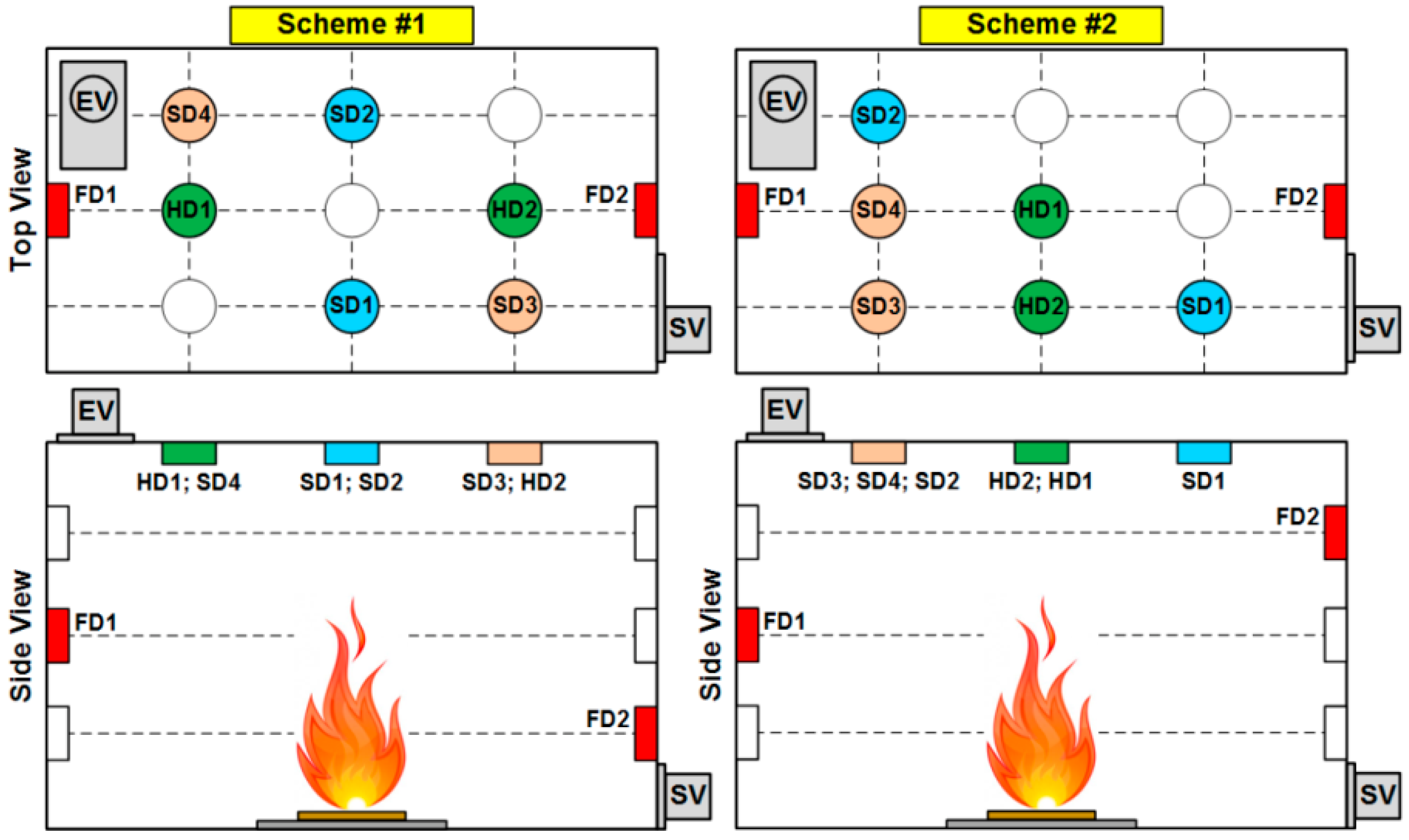
3.1. Fire Detectors
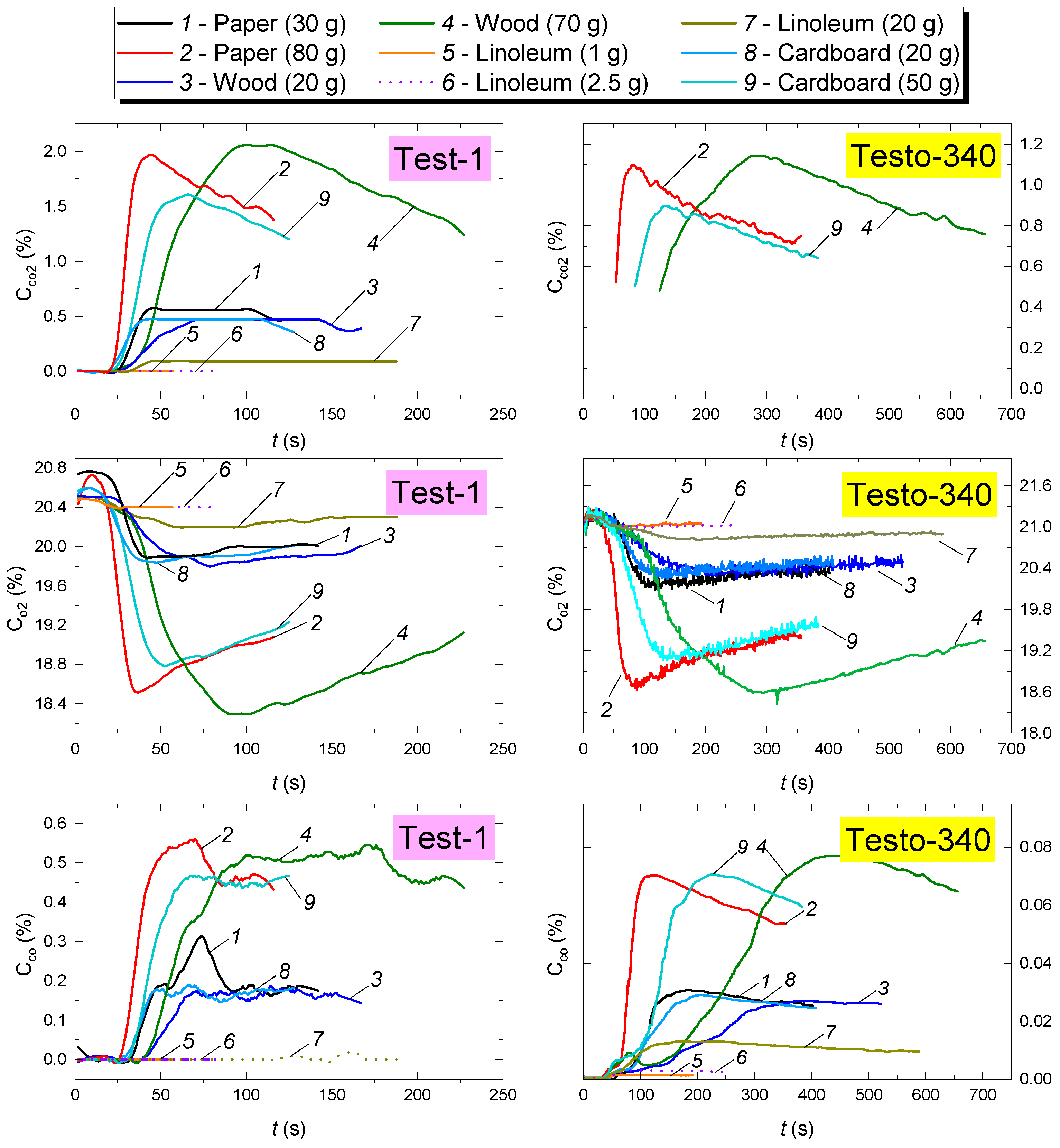
3.2. Gas Analysis
3.3. The Start Fire
- A model fire with the necessary type and mass of materials was placed into the SC;
- UProg (FACD), Owen Process Manager (DAIM), and Test and EasyEmisson (GDS) software packages were run on the PC. The fire detector (FD, HD, SD) parameters were set, along with the characteristics of analog and discrete channels of DAIM; the gas analyzer settings (GDS) were chosen;
- The model fire combustion was initiated. The PC started recording the readings of thermocouples (TC), fire detectors (FD, HD, SD) and GDS sensors. The model fire visualization was also started using the thermal imager;
- The TC, FD, HD, SD and GDS readings were recorded until the model fire stopped smoldering (which was determined by the thermal imager readings);
- The experimental results were saved on the PC, where their primary processing was performed. During processing, the following major parameters were determined: model fire surface temperature (Tf); temperature (T) at different points of the SC; complete burnout time of the model fire (tf), fire detector activation time (tD); concentrations of CO, CO2 and O2 in the SC.
3.4. Measurement Errors
4. Results and Discussion
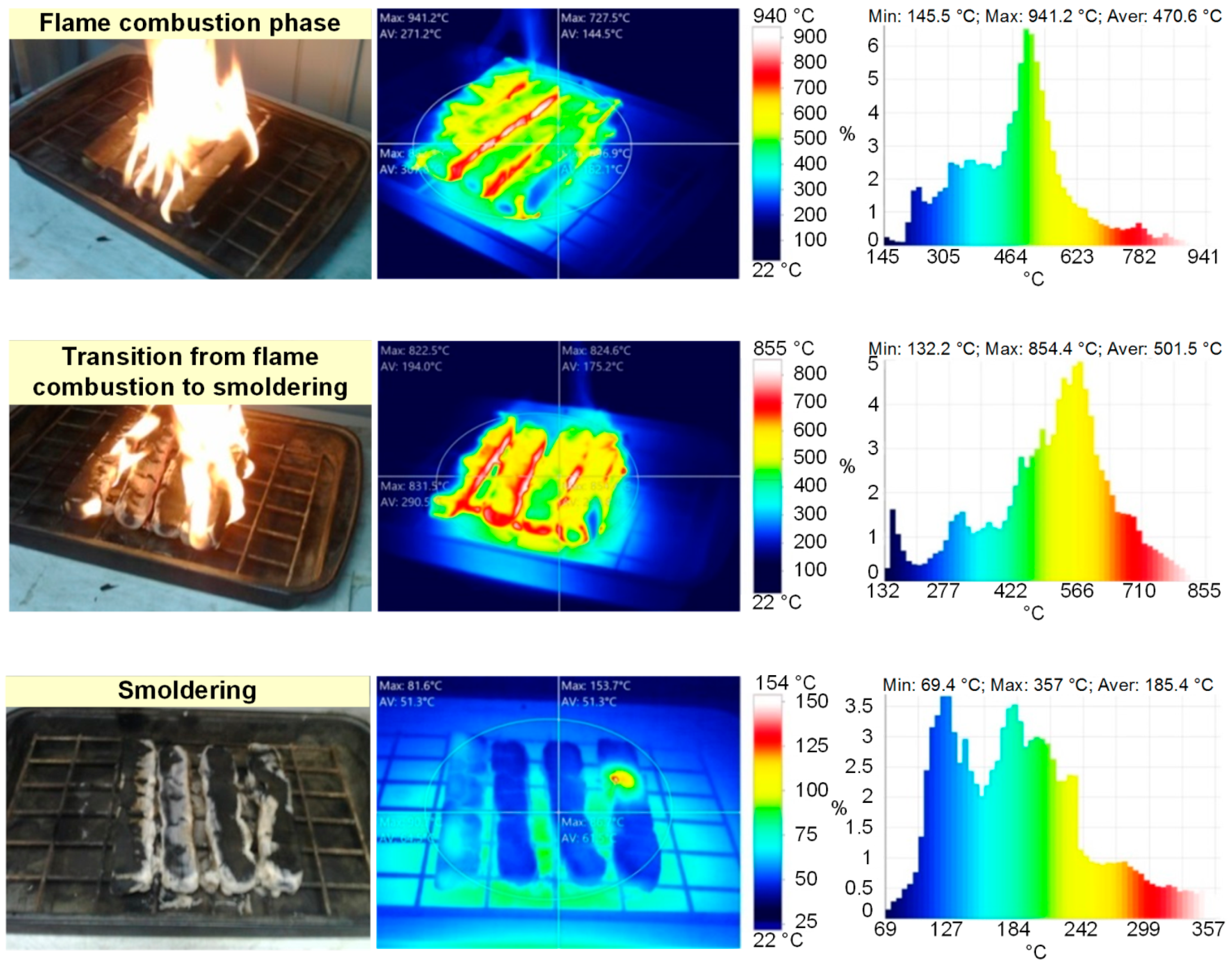
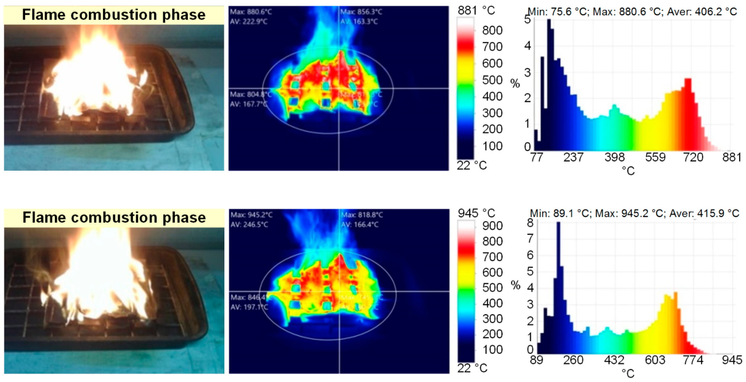
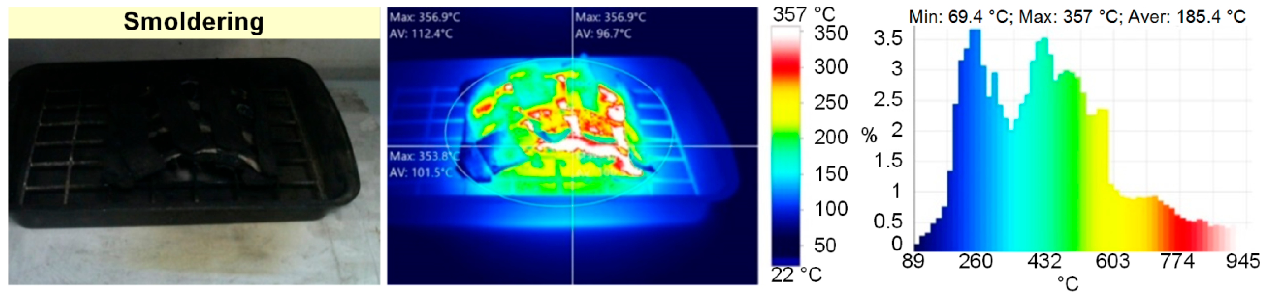
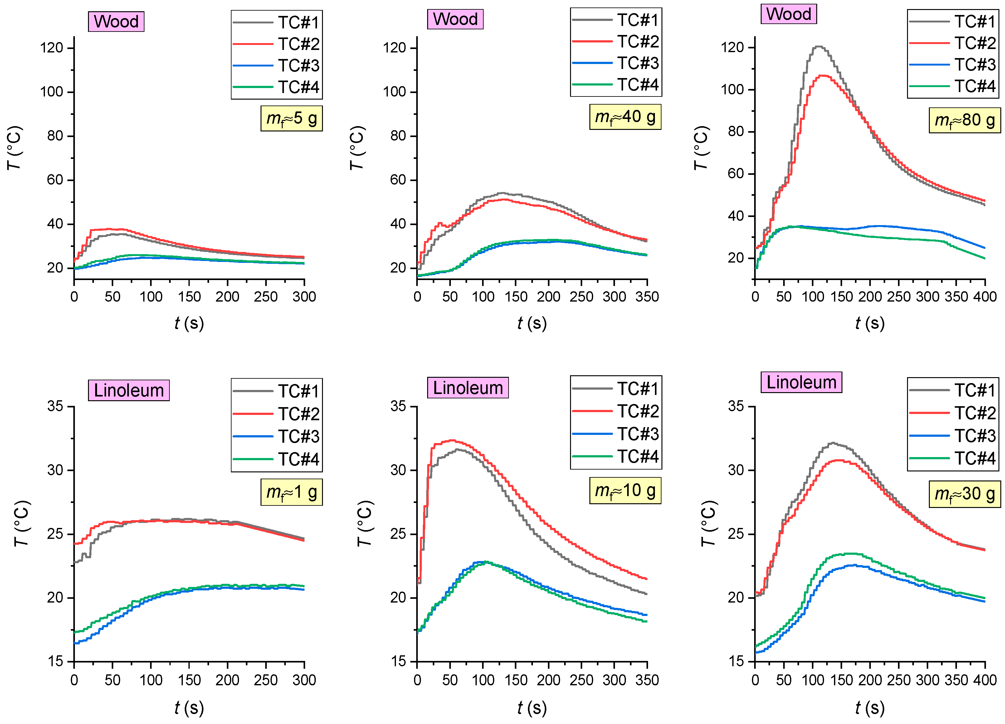
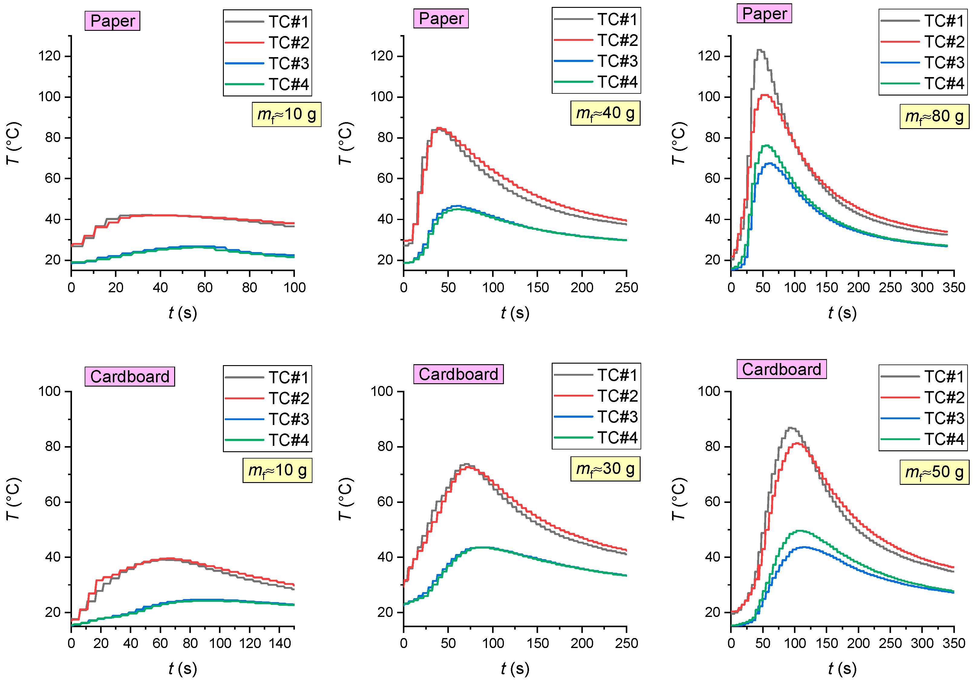
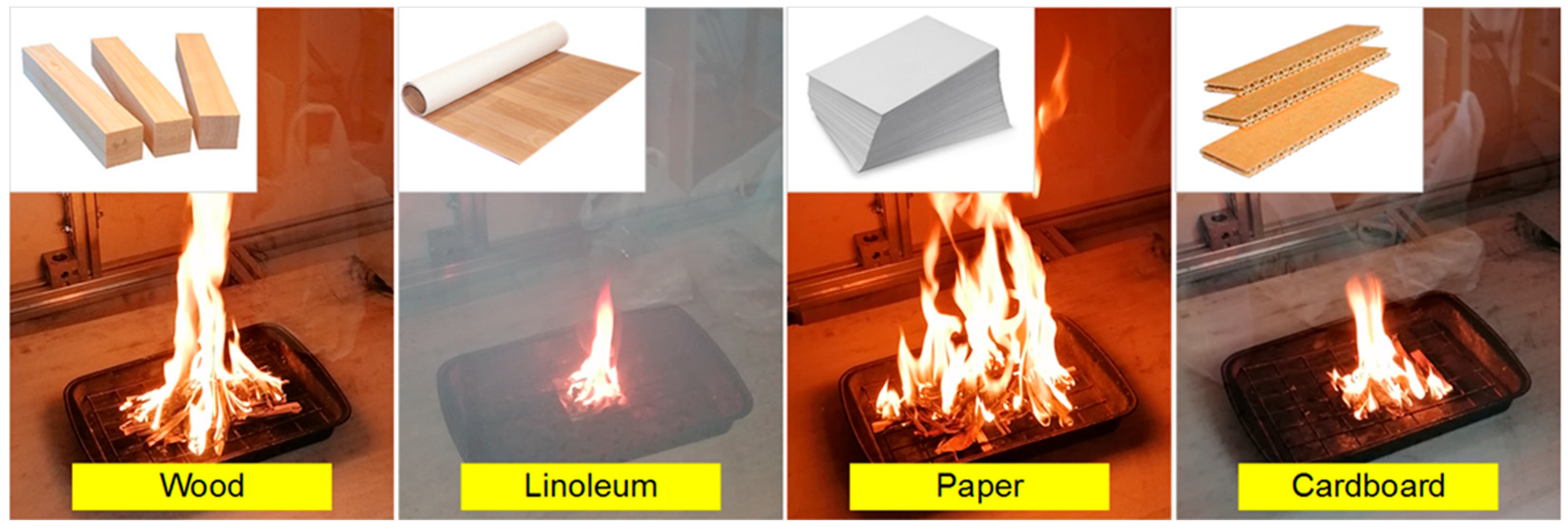
4.1. Model Fire Behavior
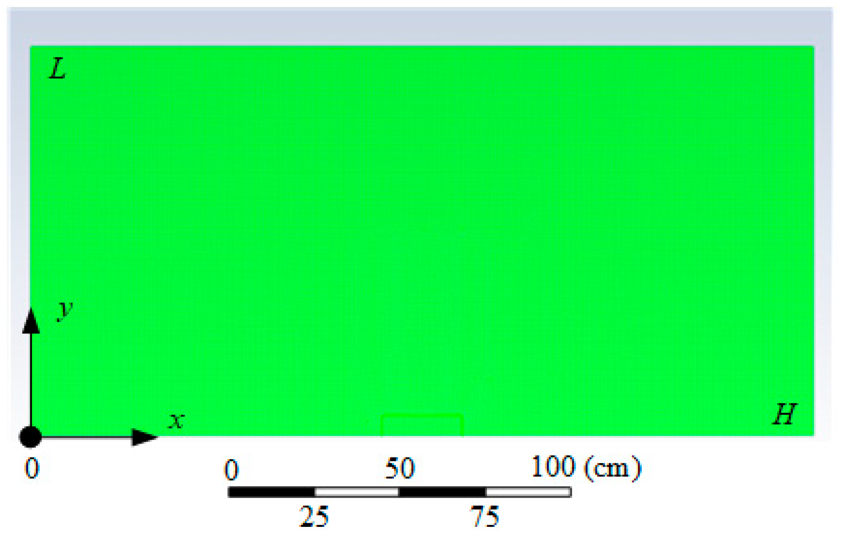
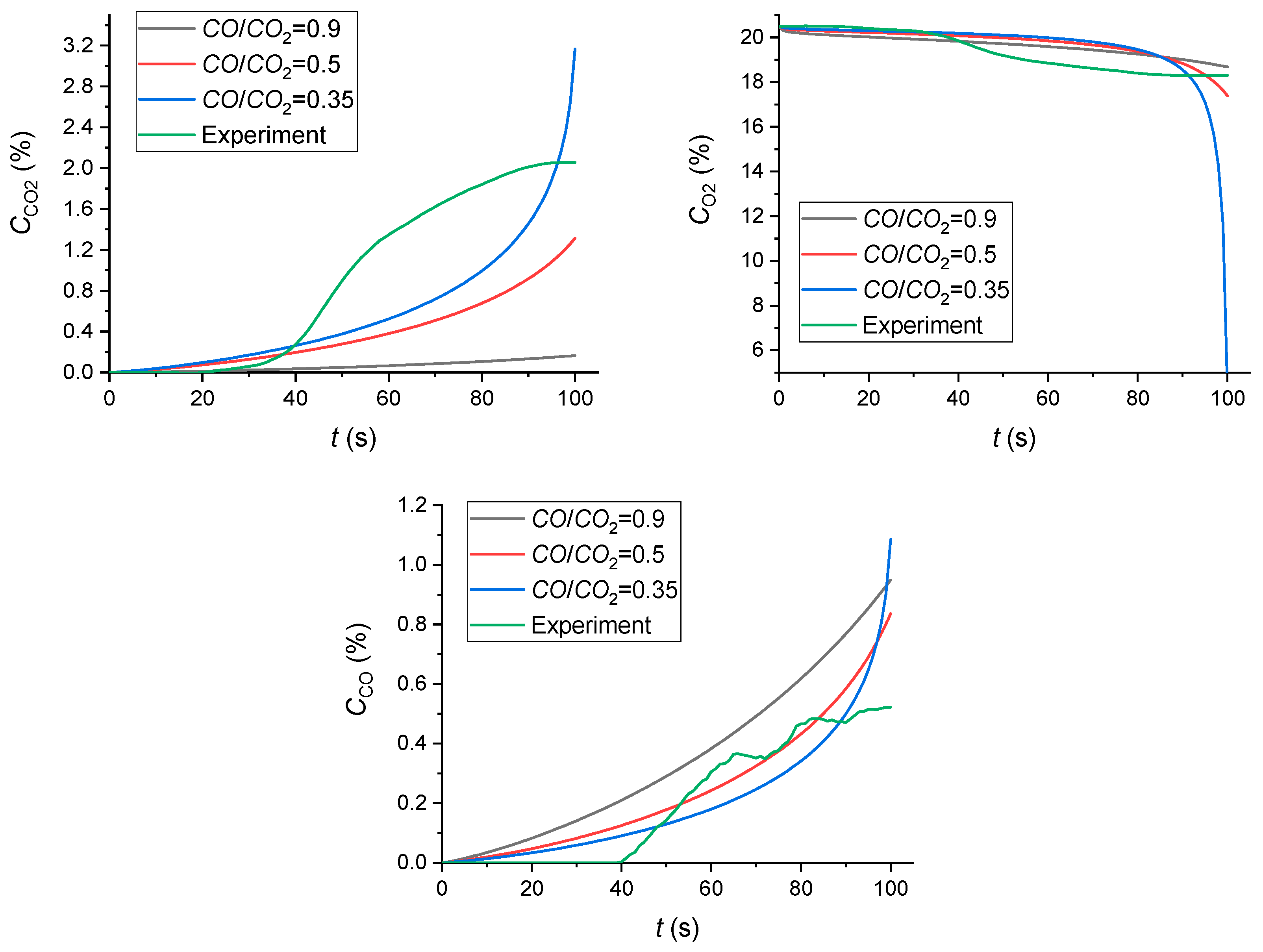
4.2. Numerical Simulation Results
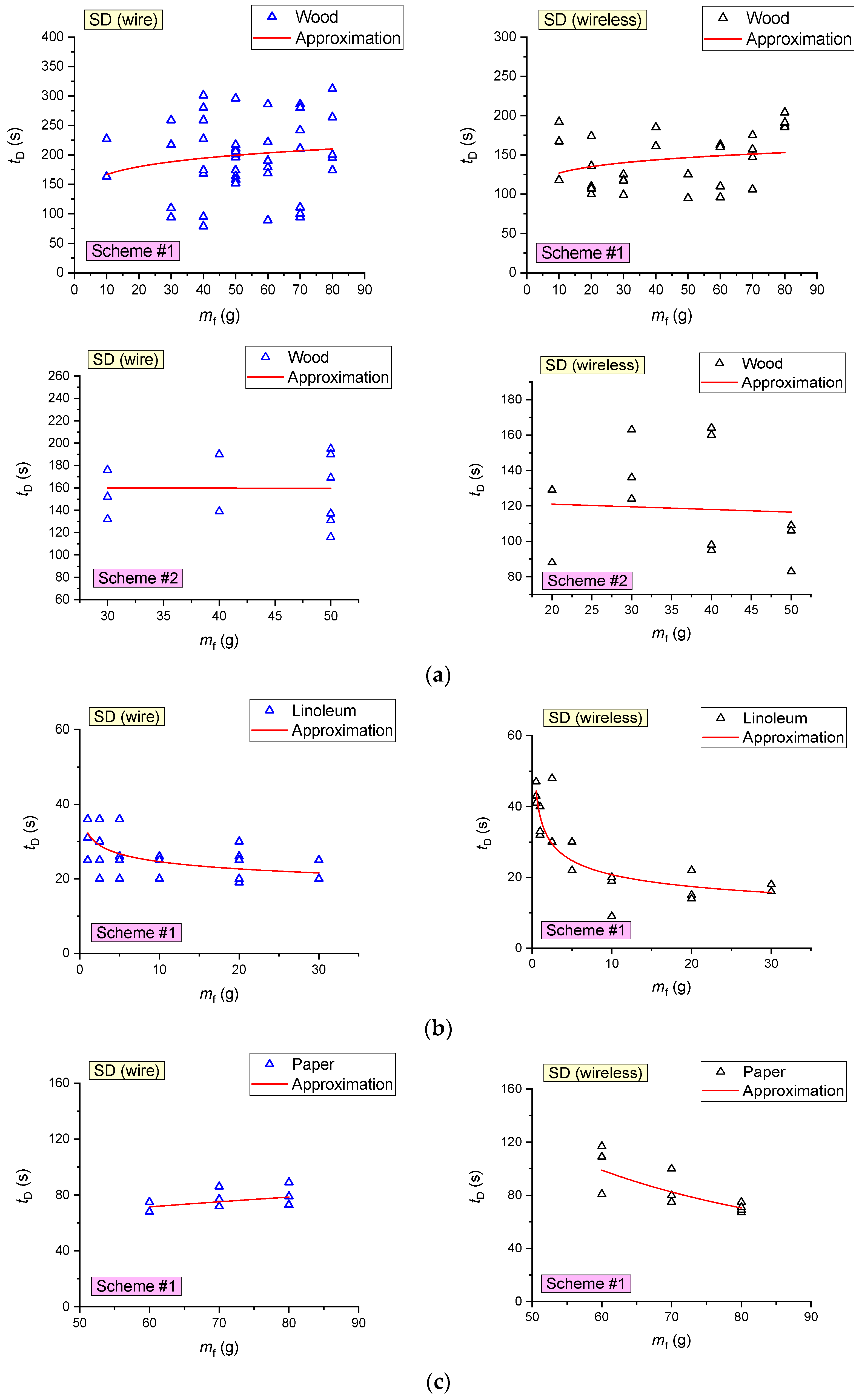
4.3. Characteristics of Fire Detector Activation
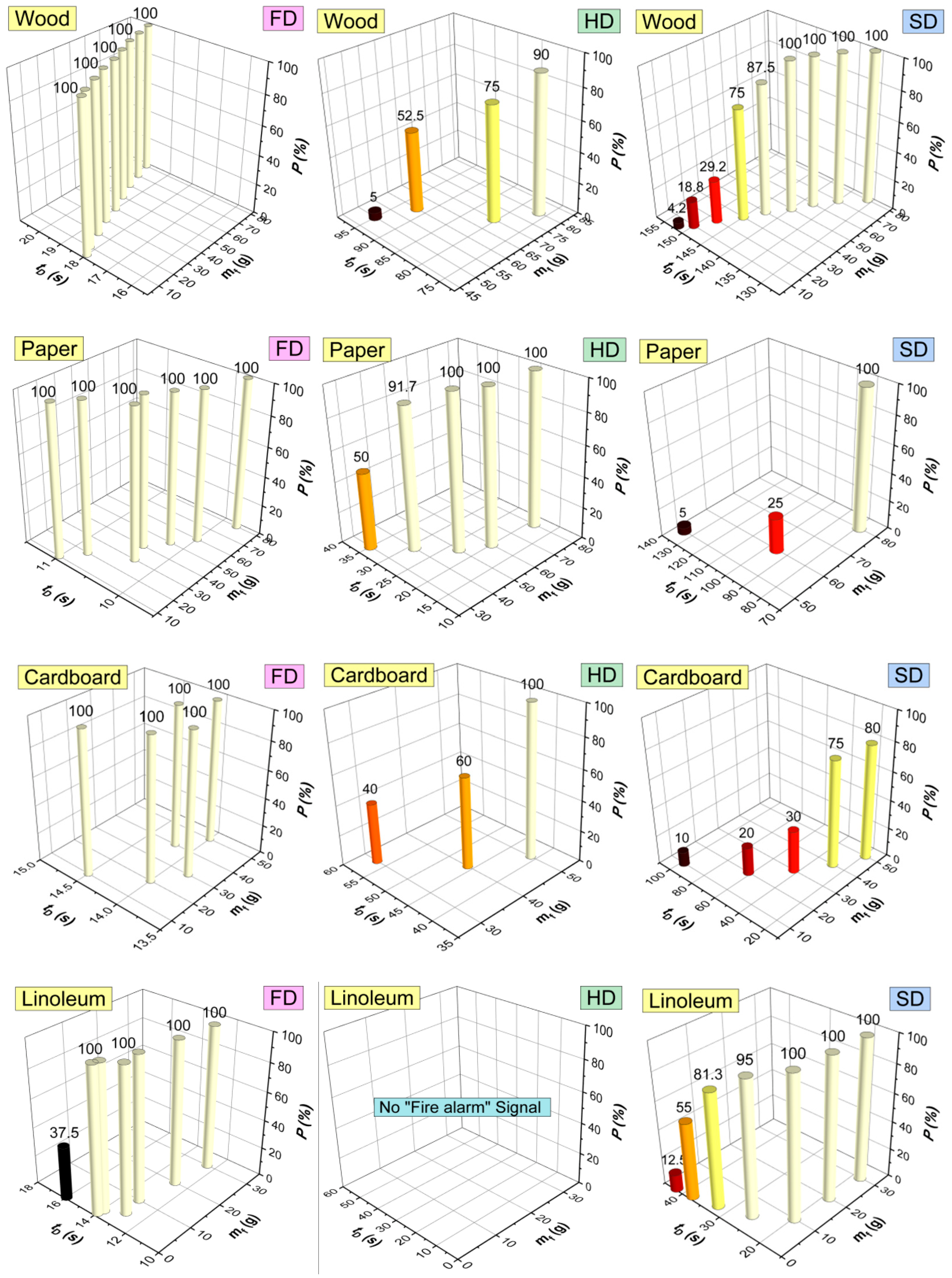
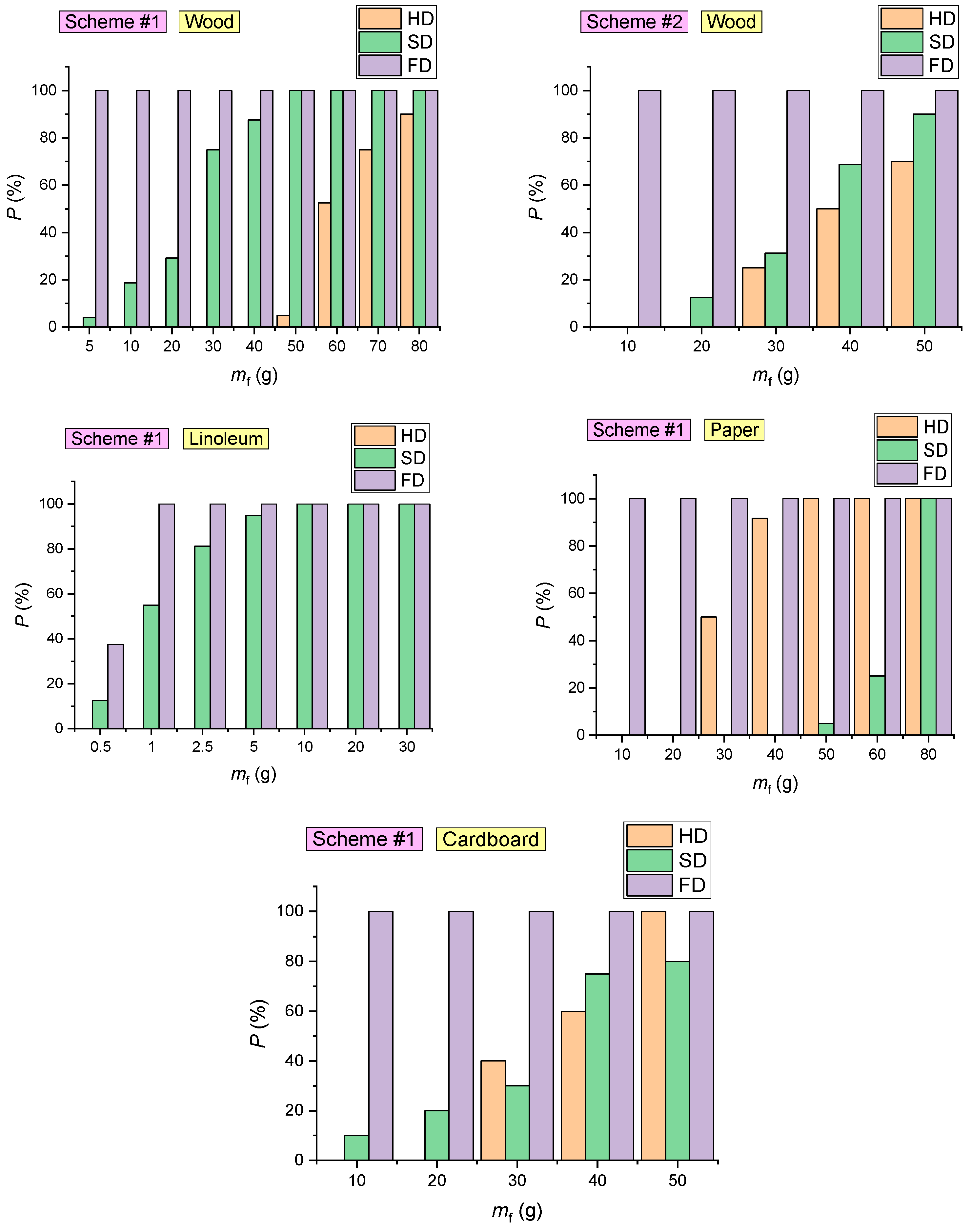
- During paper combustion, the rapid growth followed by the subsequent reduction in the temperature led to HD activation failure in 42% of cases (Figure 16), even at high rates of temperature rise (more than 1 °C/s);
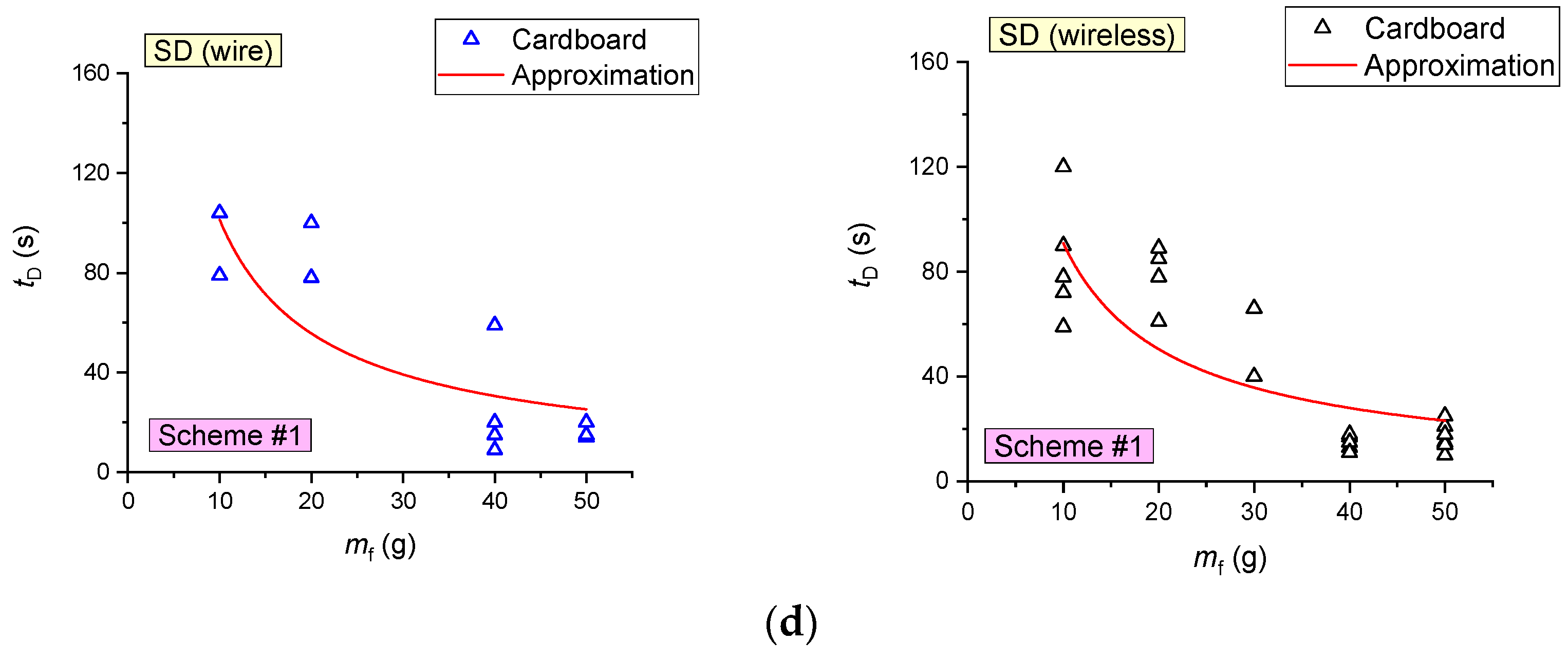
- The probability of SD activation during the combustion of cardboard (with a mass below 30 g) is less than 20%. In the combustion of cardboard with a mass exceeding 40 g, the probability of SD activation was 70–80% (Figure 19);
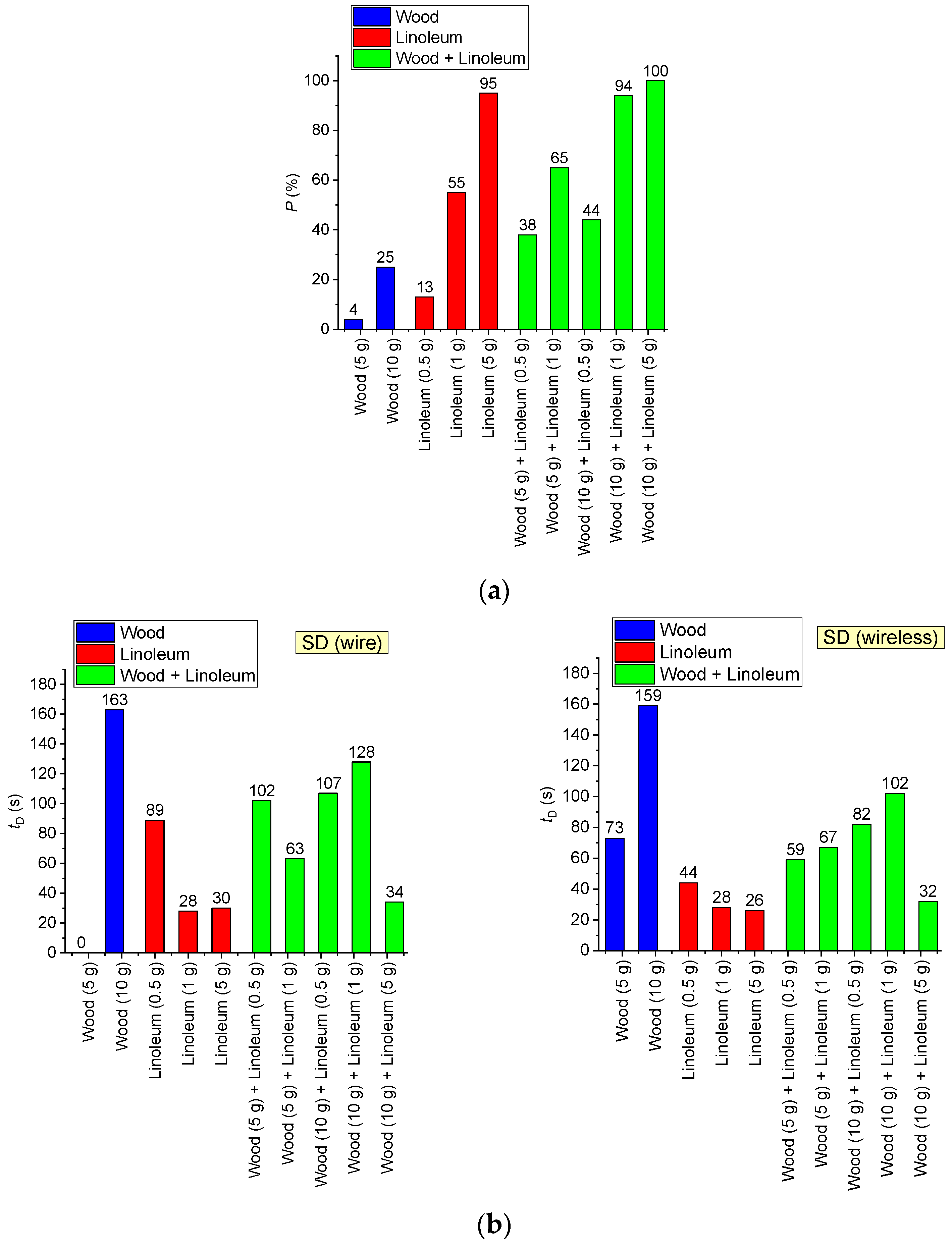
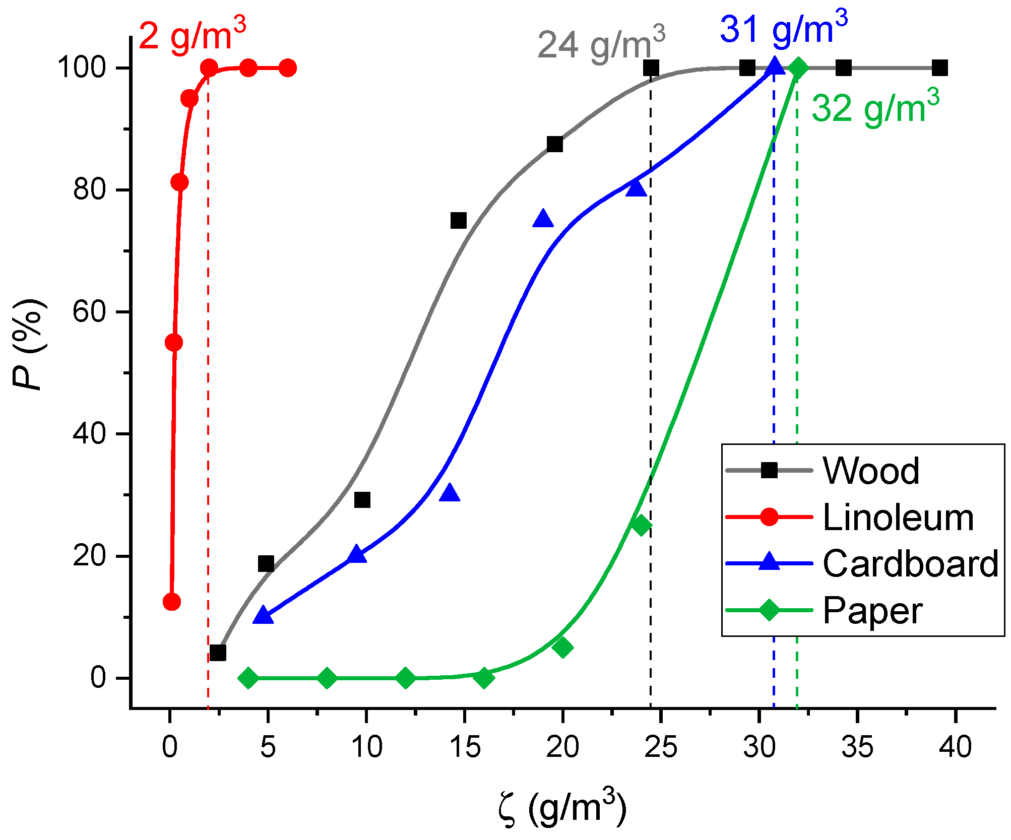
- The probability of SD activation during the combustion of 1 g fabric-backed linoleum was approximately 50%. During the combustion of linoleum with a mass of 5 g and above, the probability of SD activation reached 100% (Figure 19). This result can be explained by the intense smoke emissions of the material. At the same time, smoke particles emitted by linoleum absorb and scatter light in a wide range of wavelengths [57]. For this reason, the detectors respond quickly;
- The probability of SD activation is mainly conditioned by the type of combustible material (Figure 19);
- SDs are most effective when detecting fires involving linoleum (average detection time 28–31 s), cardboard (61 s) and wood (153–208 s);
- In the experiments conducted with the fire source located in the SC, FDs were activated in 100% cases for all the combustible materials under study (Figure 19);
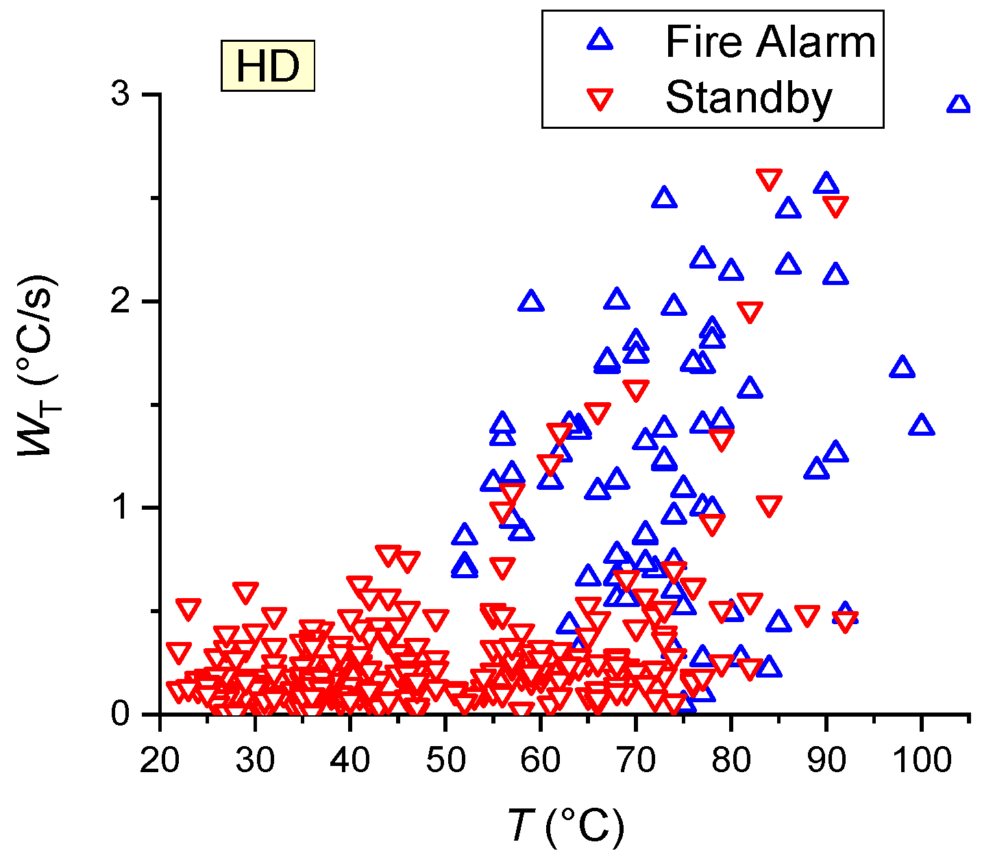
- The event of HD activation is primarily conditioned by the temperature of the gas and its growth rate (Figure 17), though the analysis in Figure 19 reveals that these parameters are indirectly affected by the mass of the sample involved in the model fire. An increase in mf contributes to faster HD activation (Figure 19).
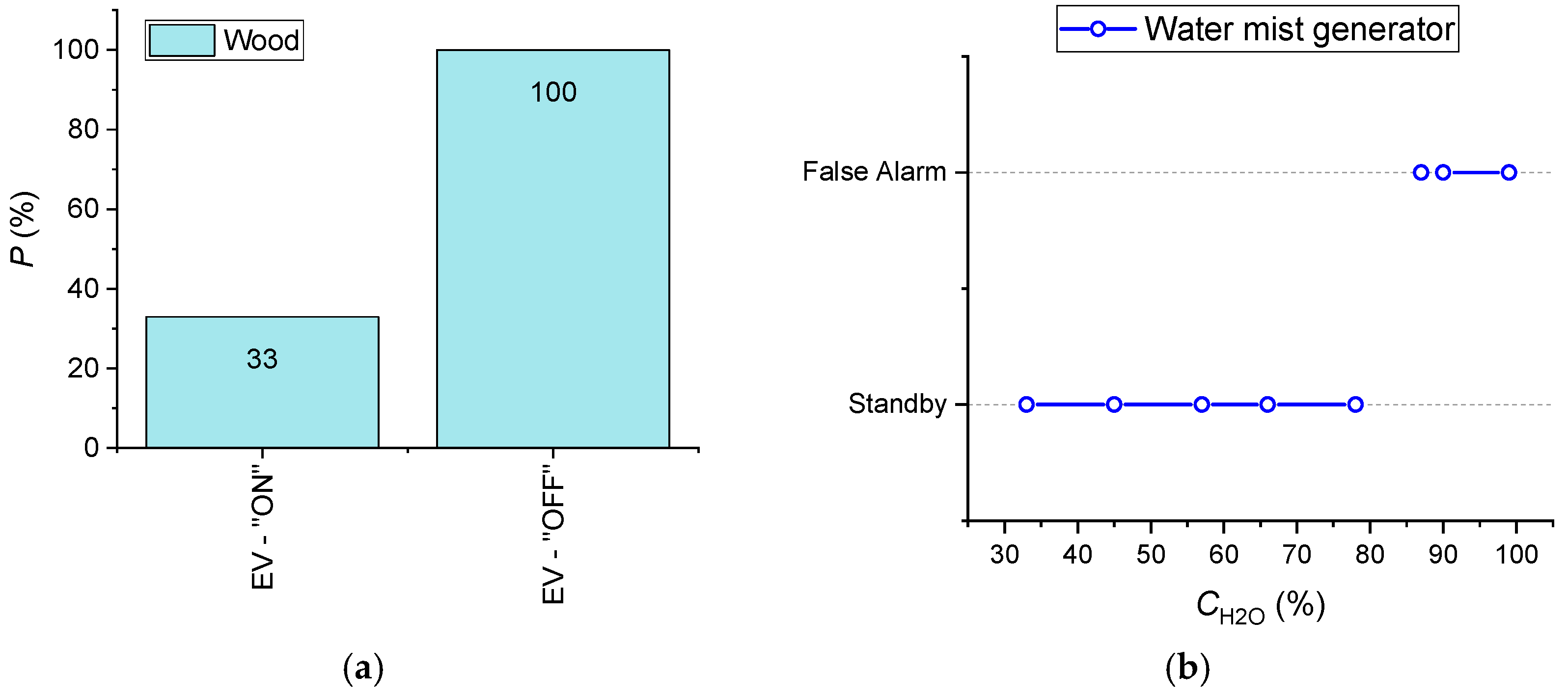
- With EV switched on and under otherwise identical conditions, the probability of SD activation decreases threefold (from 100% to 33% at the initial 100% activation) (Figure 21);
- Air humidity over 85–90% leads to false alarms of all the SD types under study (which was established in the experiments utilizing an ultrasonic water mist maker) (Figure 21). When the air humidity reaches 85–90%, the detectors are activated in 4–7 s on average;
- When a steam generator (producing hot water steam) is placed under SD (at a distance of 0.5–1 m), the detector is activated only when there is condensation (short circuit) on it in 11–12 min after the generator starts working;
- When HD is exposed to hot water steam, the detector is activated when the temperature in its vicinity reaches 63–75 °C.
5. Conclusions
- Decisive parameters for effective heat detector activation were the rate of air temperature rise, air temperature, and time that the air temperature remained sufficient for the detector to respond;
- The minimum temperature threshold for heat detector activation was 50–55 °C (at a rate of temperature rise 0.7–0.8 °C/s);
- During paper combustion, fast growth of temperature followed by its reduction led to HD activation failure in approximately 42% of cases even at high rates of temperature rise (more than 1 °C/s) and high air temperatures (over 55–60 °C);
- The most practical location of a heat detector (providing the fastest fire detection) was right above the fire;
- When a fire is located within the visual range of a flame detector, it responds to flame in 100% cases for all the combustible materials under study;
- During steady combustion of a fire (after the appearance of the flame), flame detector response time did not depend on the fuel sample mass;
- When the flame detector is moved to a distance of 1–6 m from the fire, the flame height necessary for the detector activation increased nonlinearly to 2–25 cm;
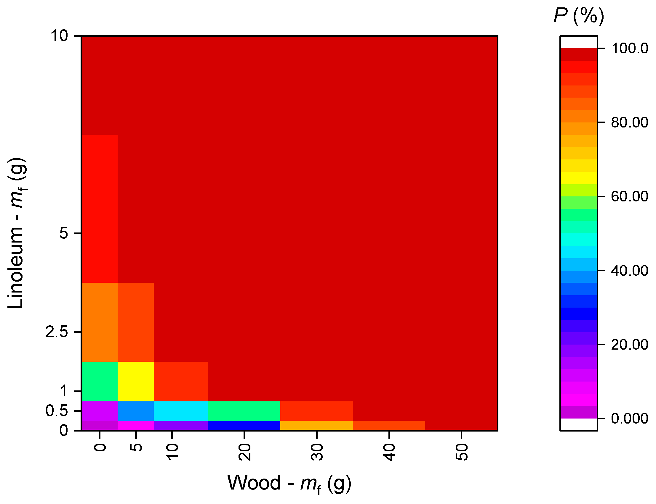
- The probability of smoke detector activation for all the combustible materials under study increased with an increase in fuel sample mass. Smoke detector activation times decreased with an increase in the mass of the combustible material;
- Smoke detectors were most effective for linoleum combustion detection;
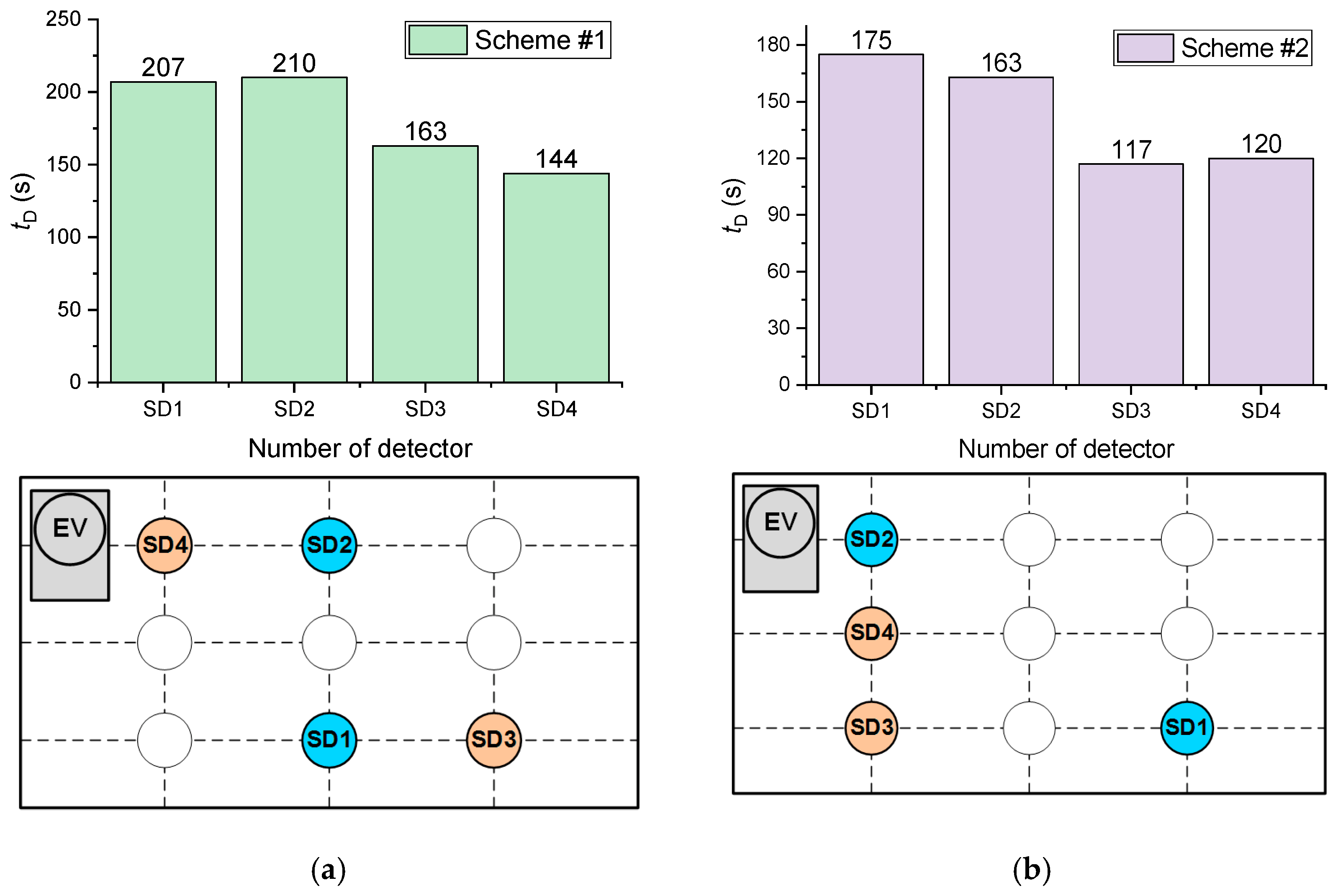
- Smoke detectors were most effective when mounted at the corner points of the ceiling. As illustrated by wired detectors connected though the circuit, the time of fire detection in this case is 20% lower than when detectors are fitted along the wall;
- With the smoke ventilation system turned on and under otherwise identical conditions, the probability of smoke detector activation decreases threefold.
Author Contributions
Funding
Conflicts of Interest
Nomenclature
| a | Temperature conductivity, m2/s |
| Ar | Pre-exponential factor of chemical reaction, s−1 |
| Cg | Heat capacity of gas, kg/m3 |
| CCO | Mass concentration (proportion) of carbon monoxide in the gas-vapor mixture, % |
| CCO2 | Mass concentration (proportion) of carbon dioxide in the gas-vapor mixture, % |
| Cf | Total mass concentration (proportion) of combustion products, % |
| CH2O | Mass concentration (proportion) of water vapors in the gas-vapor mixture, % |
| CN2 | Mass concentration (proportion) of nitrogen in the gas-vapor mixture, % |
| CO2 | Mass concentration (proportion) of oxygen in the gas-vapor mixture, % |
| D | Diffusion coefficient, m2/s |
| Df | Tentative diameter of model fire, m |
| Er | Activation energy of chemical reaction, J/mol |
| hD | Optical flame detector mounting height relative to the model fire base, m |
| hf | Height of model fire flame, m |
| H, L | Sizes of the solution domain projected to x and y axes, m |
| j | Number of experiments in a set |
| lD | Distance from the optical flame detector to the model fire, m |
| mf | Mass of materials to be burned (g) |
| na | Number of detectors of a particular type, activated in the experiment |
| nD | Total number of detectors of a particular type in the experiment |
| Nu | Nusselt number |
| P | Overall probability of activation of each type of detectors, % |
| P1, P2, …, Pj | Probability of detector activation in each experiment, % |
| Pr | Prandtl number |
| qcond | Conductive heat flux, kW/m2 |
| qconv | Convective heat flux, kW/m2 |
| qrad | Radiant heat flux, kW/m2 |
| qsum | Total heat flux, kW/m2 |
| q’ | Total heat release, kJ |
| Q | Thermal effect of chemical reaction, J/kg |
| Rt | Universal gas constant, J/(mol·K) |
| Re | Reynolds number |
| Sf | Surface areas of model fire (cm2) |
| t | Time, s |
| tD | Fire detector activation time, s |
| tf | Time of complete burnout of model fire, s |
| T | Temperature, °C |
| Tf | Temperature of model fire surface, °C |
| Tg | Gas temperature, K |
| u, v | Combustible vapor velocity components projected to x, y axes, m/s |
| Ug | Velocity (of free convection) of gas, m/s |
| W | Mass rate of chemical reaction, kg/(m3·s) |
| WT | Rate of gas temperature rise, °C/s |
| x, y | Coordinates of Cartesian system, m |
| Subscripts | |
| 1 | Gas-vapor mixture |
| i | Number of chemical reaction |
| Greek | |
| α | Convective heat transfer coefficient, W/(m2∙K) |
| βr | Exponent |
| γ | Kinematic viscosity, m/s2 |
| Δmf | Loss of mass of burning material during experiment (material pyrolysis), g |
| λg | Thermal conductivity coefficient of gas, W/(m∙K) |
| ρ | Density, kg/m3 |
| ρg | Gas density, kg/m3 |
| ψ | Stream function, m2/s |
| ω | Vorticity vector, s−1 |
| ζ | Concentration of smoke aerosol and pyrolysis products, g/m3 |
| Abbreviations | |
| DAIM | Digital and analog input module |
| EV | Exhaust ventilation |
| FACD | Fire alarm control device |
| FD | Flame detector |
| GDS | Gas detection system |
| HD | Heat detector |
| SC | Setup chamber |
| SD | Smoke detector |
| SV | Supply ventilation |
| TC | Thermocouple |
| FAC | Fire alarm circuit |
References
- Araujo Lima, G.P.; Viana Barbosa, J.D.; Beal, V.E.; Marcelo, M.A.; Souza Machado, B.A.; Gerber, J.Z.; Lazarus, B.S. Exploratory Analysis of Fire Statistical Data and Prospective Study Applied to Security and Protection Systems. Int. J. Disaster Risk Reduct. 2021, 61, 102308. [Google Scholar] [CrossRef]
- Brushlinsky, N.N.; Ahrens, M.; Sokolov, S.V. World Fire Statistics. 2020. Available online: https://www.ctif.org/sites/default/files/2020-06/CTIF_Report25.pdf (accessed on 1 May 2022).
- Shams Abadi, S.T.; Moniri Tokmehdash, N.; Hosny, A.; Nik-Bakht, M. BIM-Based Co-Simulation of Fire and Occupants’ Behavior for Safe Construction Rehabilitation Planning. Fire 2021, 4, 67. [Google Scholar] [CrossRef]
- Nazir, A.; Mosleh, H.; Takruri, M.; Jallad, A.H.; Alhebsi, H. Early Fire Detection: A New Indoor Laboratory Dataset and Data Distribution Analysis. Fire 2022, 5, 11. [Google Scholar] [CrossRef]
- Ding, Z.; Zhao, Y.; Li, A.; Zheng, Z. Spatial–Temporal Attention Two-Stream Convolution Neural Network for Smoke Region Detection. Fire 2021, 4, 66. [Google Scholar] [CrossRef]
- GOST 12.1.044–89*; Occupational Safety Standards System. Fire and Explosion Hazard of Substances and Materials. Nomenclature of Indices and Methods of Their Determination. Standardinform: Moscow, Russia, 1991.
- Bu, F.; Gharajeh, M.S. Intelligent and Vision-Based Fire Detection Systems: A Survey. Image Vis. Comput. 2019, 91, 103803. [Google Scholar] [CrossRef]
- Wu, H.; Wu, D.; Zhao, J. An Intelligent Fire Detection Approach through Cameras Based on Computer Vision Methods. Process Saf. Environ. Prot. 2019, 127, 245–256. [Google Scholar] [CrossRef]
- Hashemzadeh, M.; Zademehdi, A. Fire Detection for Video Surveillance Applications Using ICA K-Medoids-Based Color Model and Efficient Spatio-Temporal Visual Features. Expert Syst. Appl. 2019, 130, 60–78. [Google Scholar] [CrossRef]
- Khatami, A.; Mirghasemi, S.; Khosravi, A.; Lim, C.P.; Nahavandi, S. A New PSO-Based Approach to Fire Flame Detection Using K-Medoids Clustering. Expert Syst. Appl. 2017, 68, 69–80. [Google Scholar] [CrossRef]
- Hagen, B.C.; Meyer, A.K. From Smoldering to Flaming Fire: Different Modes of Transition. Fire Saf. J. 2021, 121, 103292. [Google Scholar] [CrossRef]
- Zhou, Y.; Bu, R.; Gong, J.; Zhang, X.; Fan, C.; Wang, X. Assessment of a Clean and Efficient Fire-Extinguishing Technique: Continuous and Cycling Discharge Water Mist System. J. Clean. Prod. 2018, 182, 682–693. [Google Scholar] [CrossRef]
- Zhang, X.; Zhang, Z.; Su, G.; Tang, F.; Liu, A.; Tao, H. Experimental Study on Thermal Hazard and Facade Flame Characterization Induced by Incontrollable Combustion of Indoor Energy Usage. Energy 2020, 207, 118173. [Google Scholar] [CrossRef]
- Qin, R.; Zhou, A.; Chow, C.L.; Lau, D. Structural Performance and Charring of Loaded Wood under Fire. Eng. Struct. 2021, 228, 111491. [Google Scholar] [CrossRef]
- Schmid, J.; Brandon, D.; Werther, N.; Klippel, M. Technical Note—Thermal Exposure of Wood in Standard Fire Resistance Tests. Fire Saf. J. 2019, 107, 179–185. [Google Scholar] [CrossRef]
- Zhou, Z.; Wei, Y.; Li, H.; Yuen, R.; Jian, W. Experimental Analysis of Low Air Pressure Influences on Fire Plumes. Int. J. Heat Mass Transf. 2014, 70, 578–585. [Google Scholar] [CrossRef] [Green Version]
- Mitrenga, P.; Osvaldová, L.M.; Marková, I. Observation of Fire Characteristics of Selected Covering Materials Used in Upholstered Seats. Transp. Res. Procedia 2021, 55, 1775–1782. [Google Scholar] [CrossRef]
- Zhang, Y.; Yang, X.; Luo, Y.; Gao, Y.; Liu, H.; Li, T. Experimental Study of Compartment Fire Development and Ejected Flame Thermal Behavior for a Large-Scale Light Timber Frame Construction. Case Stud. Therm. Eng. 2021, 27, 101133. [Google Scholar] [CrossRef]
- Hao, H.; Chow, C.L.; Lau, D. Effect of Heat Flux on Combustion of Different Wood Species. Fuel 2020, 278, 118325. [Google Scholar] [CrossRef]
- Diab, M.T.; Haelssig, J.B.; Pegg, M.J. The Behaviour of Wood Crib Fires under Free Burning and Fire Whirl Conditions. Fire Saf. J. 2020, 112, 102941. [Google Scholar] [CrossRef]
- Tao, L.; Zeng, Y. Effect of Different Smoke Vent Layouts on Smoke and Temperature Distribution in Single-Side Multi-Point Exhaust Tunnel Fires: A Case Study. Fire 2022, 5, 28. [Google Scholar] [CrossRef]
- Qiu, X.; Wei, Y.; Li, N.; Guo, A.; Zhang, E.; Li, C.; Peng, Y.; Wei, J.; Zang, Z. Development of an Early Warning Fire Detection System Based on a Laser Spectroscopic Carbon Monoxide Sensor Using a 32-Bit System-on-Chip. Infrared Phys. Technol. 2019, 96, 44–51. [Google Scholar] [CrossRef]
- Li, Y.Z.; Ingason, H. Influence of Fire Suppression on Combustion Products in Tunnel Fires. Fire Saf. J. 2018, 97, 96–110. [Google Scholar] [CrossRef] [Green Version]
- Pan, W.; Zhang, M.; Gao, X.; Mo, S. Establishment of Aqueous Film Forming Foam Extinguishing Agent Minimum Supply Intensity Model Based on Experimental Method. J. Loss Prev. Process Ind. 2020, 63, 103997. [Google Scholar] [CrossRef]
- Bustamante Valencia, L.; Rogaume, T.; Guillaume, E.; Rein, G.; Torero, J.L. Analysis of Principal Gas Products during Combustion of Polyether Polyurethane Foam at Different Irradiance Levels. Fire Saf. J. 2009, 44, 933–940. [Google Scholar] [CrossRef] [Green Version]
- Bluvshtein, N.; Villacorta, E.; Li, C.; Hagen, B.C.; Frette, V.; Rudich, Y. Early Detection of Smoldering in Silos: Organic Material Emissions as Precursors. Fire Saf. J. 2020, 114, 103009. [Google Scholar] [CrossRef]
- Noaki, M.; Delichatsios, M.A.; Yamaguchi, J.; Ohmiya, Y. Heat Release Rate of Wooden Cribs with Water Application for Fire Suppression. Fire Saf. J. 2018, 95, 170–179. [Google Scholar] [CrossRef]
- Gorska, C.; Hidalgo, J.P.; Torero, J.L. Fire Dynamics in Mass Timber Compartments. Fire Saf. J. 2021, 120, 103098. [Google Scholar] [CrossRef]
- Östman, B.; Brandon, D.; Frantzich, H. Fire Safety Engineering in Timber Buildings. Fire Saf. J. 2017, 91, 11–20. [Google Scholar] [CrossRef] [Green Version]
- Onorati, T.; Malizia, A.; Diaz, P.; Aedo, I. Modeling an Ontology on Accessible Evacuation Routes for Emergencies. Expert Syst. Appl. 2014, 41, 7124–7134. [Google Scholar] [CrossRef] [Green Version]
- Wagner, N.; Agrawal, V. An Agent-Based Simulation System for Concert Venue Crowd Evacuation Modeling in the Presence of a Fire Disaster. Expert Syst. Appl. 2014, 41, 2807–2815. [Google Scholar] [CrossRef]
- GOST R 51032–97; Building Materials. Spread Flame Test Method. Standardinform: Moscow, Russia, 1997.
- Lowden, L.A.; Hull, T.R. Flammability Behaviour of Wood and a Review of the Methods for Its Reduction. Fire Sci. Rev. 2013, 2, 4. [Google Scholar] [CrossRef] [Green Version]
- Log, T. Cold Climate Fire Risk; A Case Study of the Lærdalsøyri Fire, January 2014. Fire Technol. 2016, 52, 1825–1843. [Google Scholar] [CrossRef] [Green Version]
- Toscano, G.; Leoni, E.; Gasperini, T.; Picchi, G. Performance of a Portable NIR Spectrometer for the Determination of Moisture Content of Industrial Wood Chips Fuel. Fuel 2022, 320, 123948. [Google Scholar] [CrossRef]
- Park, J.; Kwark, J. Experimental Study on Fire Sources for Full-Scale Fire Testing of Simple Sprinkler Systems Installed in Multiplexes. Fire 2021, 4, 8. [Google Scholar] [CrossRef]
- GOST R 54081-2010 (MEK 60721-2-8:1994); Influence of Environmental Conditions Appearing in Nature on the Technical Products. Overall Performance Fire. Standardinform: Moscow, Russia, 2011.
- Pitarma, R.; Crisóstomo, J. Determination of Wood Emissivity Using Active Infrared Thermography. In Environmental Science and Engineering; Springer: Berlin/Heidelberg, Germany, 2021. [Google Scholar]
- Touloukian, Y.S.; Powell, R.W.; Ho, C.Y.; Klemens, P.G. Thermophysical Properties of Matter—The TPRC Data Series; Thermophysical and Electronic Properties Information Center: Lafayette, IN, USA, 1975. [Google Scholar]
- Yakimovich, K.A. Thermophysical Properties of Materials. Phys. Technol. 1977, 8, 35–36. [Google Scholar] [CrossRef] [Green Version]
- Kuznetsov, G.V.; Piskunov, M.V.; Volkov, R.S.; Strizhak, P.A. Unsteady Temperature Fields of Evaporating Water Droplets Exposed to Conductive, Convective and Radiative Heating. Appl. Therm. Eng. 2018, 131, 340–355. [Google Scholar] [CrossRef]
- Horvat, A.; Sinai, Y.; Pearson, A.; Most, J.M. Contribution to Flashover Modelling: Development of a Validated Numerical Model for Ignition of Non-Contiguous Wood Samples. Fire Saf. J. 2009, 44, 779–788. [Google Scholar] [CrossRef]
- Terrei, L.; Acem, Z.; Marchetti, V.; Lardet, P.; Boulet, P.; Parent, G. In-Depth Wood Temperature Measurement Using Embedded Thin Wire Thermocouples in Cone Calorimeter Tests. Int. J. Therm. Sci. 2021, 162, 106686. [Google Scholar] [CrossRef]
- Gollner, M.J.; Overholt, K.; Williams, F.A.; Rangwala, A.S.; Perricone, J. Warehouse Commodity Classification from Fundamental Principles. Part I: Commodity & Burning Rates. Fire Saf. J. 2011, 46, 305–316. [Google Scholar] [CrossRef]
- He, Q.; Liu, N.; Xie, X.; Zhang, L.; Zhang, Y.; Yan, W. Experimental Study on Fire Spread over Discrete Fuel Bed-Part I: Effects of Packing Ratio. Fire Saf. J. 2021, 126, 103470. [Google Scholar] [CrossRef]
- Vershinina, K.; Shabardin, D.; Strizhak, P. Burnout Rates of Fuel Slurries Containing Petrochemicals, Coals and Coal Processing Waste. Powder Technol. 2019, 343, 204–214. [Google Scholar] [CrossRef]
- Glushkov, D.O.; Lyrshchikov, S.Y.; Shevyrev, S.A.; Strizhak, P.A. Burning Properties of Slurry Based on Coal and Oil Processing Waste. Energy Fuels 2016, 30, 3441–3450. [Google Scholar] [CrossRef]
- Ansys Fluent Theory Guide Ansys Fluent Theory Guide; ANSYS Inc.: Canonsburg, PA, USA, 2021.
- You, J.; Huai, Y.; Nie, X.; Chen, Y. Real-Time 3D Visualization of Forest Fire Spread Based on Tree Morphology and Finite State Machine. Comput. Graph. 2022, 103, 109–120. [Google Scholar] [CrossRef]
- Frangieh, N.; Accary, G.; Rossi, J.L.; Morvan, D.; Meradji, S.; Marcelli, T.; Chatelon, F.J. Fuelbreak Effectiveness against Wind-Driven and Plume-Dominated Fires: A 3D Numerical Study. Fire Saf. J. 2021, 124, 103383. [Google Scholar] [CrossRef]
- Konovalov, I.B.; Golovushkin, N.A.; Beekmann, M.; Andreae, M.O. Insights into the Aging of Biomass Burning Aerosol from Satellite Observations and 3D Atmospheric Modeling: Evolution of the Aerosol Optical Properties in Siberian Wildfire Plumes. Atmos. Chem. Phys. 2021, 21, 357–392. [Google Scholar] [CrossRef]
- Tavakolian, Z.; Abouali, O.; Yaghoubi, M. 3D Simulations of Smoke Exhaust System in Two Types of Subway Station Platforms. Int. J. Vent. 2021, 20, 65–81. [Google Scholar] [CrossRef]
- Bao, T.; Liu, S.; Qin, Y.; Liu, L.Z. 3D Modeling of Coupled Soil Heat and Moisture Transport beneath a Surface Fire. Int. J. Heat Mass Transf. 2020, 149, 119163. [Google Scholar] [CrossRef]
- Baranovskiy, N.V. Algorithms for Parallelizing a Mathematical Model of Forest Fires on Supercomputers and Theoretical Estimates for the Efficiency of Parallel Programs. Cybern. Syst. Anal. 2015, 51, 471–480. [Google Scholar] [CrossRef]
- Li, J.; Li, X.; Chen, C.; Zheng, H.; Liu, N. Three-Dimensional Dynamic Simulation System for Forest Surface Fire Spreading Prediction. Int. J. Pattern Recognit. Artif. Intell. 2018, 32, 1850026. [Google Scholar] [CrossRef]
- Hurley, M.J.; Gottuk, D.; Hall, J.R.; Harada, K.; Kuligowski, E.; Puchovsky, M.; Torero, J.; Watts, J.M.; Wieczorek, C. Handbook of Fire Protection Engineering, 5th ed.; SFPE: Quincy, MA, USA, 2016; ISBN 9781493925650. [Google Scholar]
- Zhdanova, A.O.; Volkov, R.S.; Kuznetsov, G.V.; Kopylov, N.P.; Kopylov, S.N.; Syshkina, E.Y.; Strizhak, P.A. Solid particle deposition of indoor material combustion products. Process Saf. Environ. Prot. 2022, 162, 494–512. [Google Scholar] [CrossRef]


| No. | Indicator | State of Matter of Substances and Materials | |||
|---|---|---|---|---|---|
| Gases (10) | Liquids (14) | Solids (9) | Dust (11) | ||
| 1 | Autoignition temperature | + | |||
| 2 | Explosiveness and combustibility when interacting with water, oxygen and other substances | + | |||
| 3 | Ignition temperature | + | |||
| 4 | Flammability limits | + | + | ||
| 5 | Minimum ignition energy | + | + | ||
| 6 | Minimum explosion-hazardous content of oxygen | + | + | ||
| 7 | Minimum concentration of phlegmatized explosive | + | + | ||
| 8 | Maximum explosion pressure | + | + | ||
| 9 | Rate of explosion pressure rise | + | + | ||
| 10 | Diffusion flame limits of gas mixtures in the air | + | |||
| 11 | Normal burning rate | + | |||
| 12 | Smoldering temperature | + | |||
| 13 | Thermal autoignition conditions | + | |||
| 14 | Flash temperature | + | |||
| 15 | Temperature limits of flame spread (ignition) | + | |||
| 16 | Burnout rate | + | |||
| 17 | Oxygen index | + | |||
| 18 | Smoke generation coefficient | + | |||
| 19 | Flame spread index | + | |||
| 20 | Decomposition product toxicity indicator | + | |||
| Material | Characteristics | Limit Mass of Materials to Be Burned, g |
|---|---|---|
| Pine wood | Pine density is 520 kg/m3 at a humidity of 12–15%. Total heat of combustion of pine wood is 4.4 kW·h/kg. The combustion of pine wood produces water vapor, heat, carbon dioxide and carbon monoxide, aldehydes, acids and different gases. | 90 |
| Fabric backed linoleum | Linoleum backed with fabric is made of polyvinyl chloride with plasticizers, fillers and dyes. A quality material does not support active combustion. The main combustion product of polyvinyl chloride is hydrogen chloride. | 30 |
| Class A paper | The density of class A paper is 80 g/m2 (800 kg/m3). Its combustion proceeds with heat release and produces carbon dioxide, carbon monoxide and water vapor. | 50 |
| Corrugated cardboard | It is mainly made up of recycled materials (semicellulose, straw, waste paper, etc.) The rest are primary cellulose fibers. | 50 |
| Gas-Air Mixture Component | Type of Sensors | Measurement Range | Accuracy | Response Time |
|---|---|---|---|---|
| Test 1 gas analyzer | ||||
| O2 | electrochemical | 0–25% | ±0.2 vol% (absolute) | ≤15 s |
| H2 | polarographic | 0–5% | ±0.2 vol% (absolute) | ≤35 s |
| CO2 | optical | 0–30% | ±2% (basic percentage error) | ≤25 s |
| CH4 | optical | 0–30% | ±5% (relative) | ≤25 s |
| CO | electrochemical | 0–40,000 ppm | ±5% (relative) | ≤35 s |
| CO | electrochemical | 0–4000 ppm | ±5% (relative) | ≤35 s |
| NO | electrochemical | 0–1000 ppm | ±5% (relative) | ≤35 s |
| NO2 | electrochemical | 0–500 ppm | ±7% (relative) | ≤45 s |
| H2S | electrochemical | 0–500 ppm | ±7% (relative) | ≤45 s |
| SO2 | electrochemical | 0–1000 ppm | ±5% (relative) | ≤45 s |
| Test-340 gas analyzer | ||||
| O2 | electrochemical | 0–25 vol% | ±0.2 vol% | <20 s |
| CO | electrochemical | 0–10,000 ppm | ±10% of measured value | <40 s |
| NOx | electrochemical | 0–4000 ppm | ±5 ppm (0–99 ppm) ±5% of measured value (100–1999 ppm) | <30 s |
| SO2 | electrochemical | 0–5000 ppm | ±10 ppm (0–99 ppm) | <40 s |
| CO2 | – | 0–CO2max | ±0.2 vol% | <40 s |
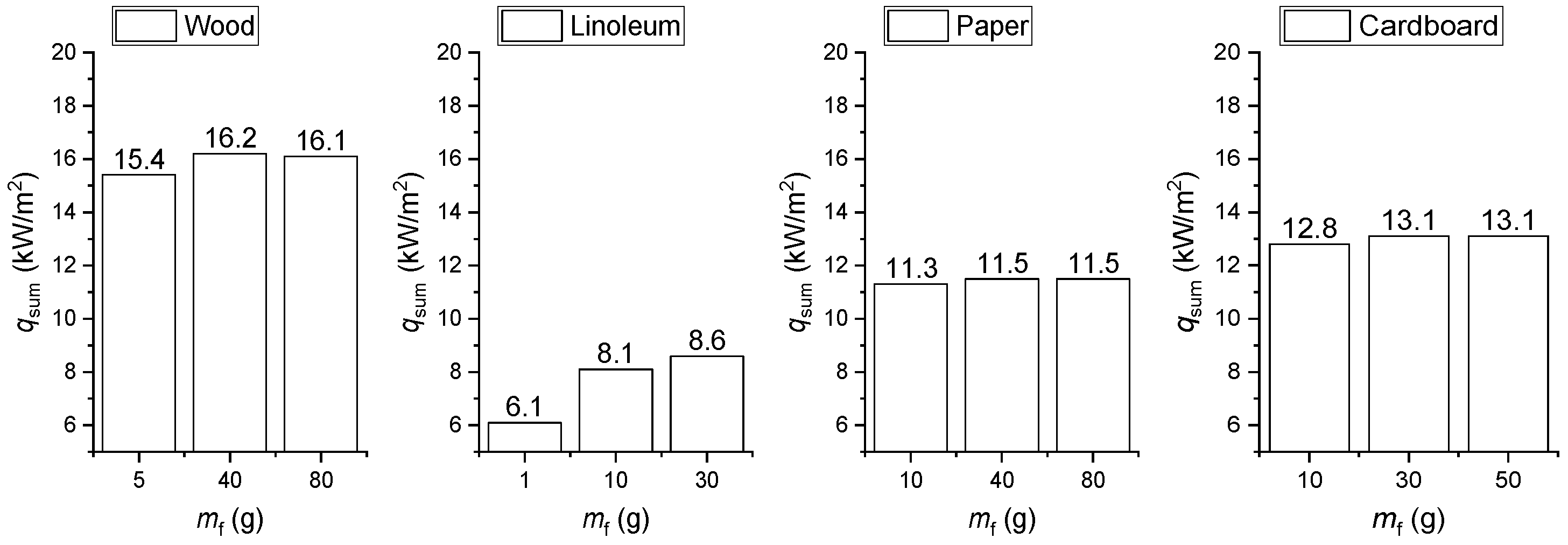
| Material Involved in the Fire | qconv (kW/m2) | qcond (kW/m2) | qrad (kW/m2) | qsum (kW/m2) |
|---|---|---|---|---|
| Wood | 2.92–1.31 | 0.08–0.24 | 17.34–18.07 | 15.38–16.58 |
| Linoleum | 4.79–1.70 | 0.12–0.63 | 10.14–10.20 | 6.09–8.58 |
| Paper | 1.68–0.73 | 0.04–0.10 | 12.15–12.92 | 11.29–12.03 |
| Cardboard | 1.76–0.91 | 0.04–0.11 | 13.99–14.50 | 12.80–13.48 |
| Material Involved in the Fire | Specific Heat Flux qsum, kW/m2 | |||
|---|---|---|---|---|
| Findings of This Research | [42] | [44] | [45] | |
| Wood | 15.38–16.58 | 18–21 | – | – |
| Cardboard | 12.80–13.48 | – | 5.30 | 11 |
| No. | Reaction | CO/CO2 | Q, MJ/kg | Ari, s−1 | βr | Er, J/mol |
|---|---|---|---|---|---|---|
| 1 | 0.9 | 24 | 1.349 × 10¹⁰ | 0 | 2.997 × 10⁸ | |
| 2 | 0.5 | |||||
| 3 | 0.35 | |||||
| 2 | 2.239 × 10¹⁰ | 0 | 8.7 × 10⁸ |
| Parameter or Factor | Activation/Time of Activation | ||
|---|---|---|---|
| FD | HD | SD | |
| Material (or a combination of materials) involved in the fire | − | − | + |
| Mass of burning materials | − | ± | + |
| Fire area | − | ± | − |
| Flame height | + | ± | − |
| Duration of flame combustion | − | ± | ± |
| Gas temperature | − | + | − |
| Rate of gas temperature rise | − | + | − |
| Gas humidity | − | − | + |
| Detector location | + | + | + |
| Availability of supply and exhaust ventilation | − | − | + |
Publisher’s Note: MDPI stays neutral with regard to jurisdictional claims in published maps and institutional affiliations. |
© 2022 by the authors. Licensee MDPI, Basel, Switzerland. This article is an open access article distributed under the terms and conditions of the Creative Commons Attribution (CC BY) license (https://creativecommons.org/licenses/by/4.0/).
Share and Cite
Zhdanova, A.; Volkov, R.; Sviridenko, A.; Kuznetsov, G.; Strizhak, P. Influence of Compartment Fire Behavior at Ignition and Combustion Development Stages on the Operation of Fire Detectors. Fire 2022, 5, 84. https://doi.org/10.3390/fire5030084
Zhdanova A, Volkov R, Sviridenko A, Kuznetsov G, Strizhak P. Influence of Compartment Fire Behavior at Ignition and Combustion Development Stages on the Operation of Fire Detectors. Fire. 2022; 5(3):84. https://doi.org/10.3390/fire5030084
Chicago/Turabian StyleZhdanova, Alena, Roman Volkov, Aleksandr Sviridenko, Geniy Kuznetsov, and Pavel Strizhak. 2022. "Influence of Compartment Fire Behavior at Ignition and Combustion Development Stages on the Operation of Fire Detectors" Fire 5, no. 3: 84. https://doi.org/10.3390/fire5030084
APA StyleZhdanova, A., Volkov, R., Sviridenko, A., Kuznetsov, G., & Strizhak, P. (2022). Influence of Compartment Fire Behavior at Ignition and Combustion Development Stages on the Operation of Fire Detectors. Fire, 5(3), 84. https://doi.org/10.3390/fire5030084