Article

Mapping Wetland Burned Area from Sentinel-2 across the Southeastern United States and Its Contributions Relative to Landsat-8 (2016–2019)

1
U.S. Geological Survey, Geosciences and Environmental Change Science Center, Denver Federal Center, MS980, Denver, CO 80225, USA
2
US Fish and Wildlife Service, Fire Management Branch, 3833 S Development Ave., Boise, ID 83705, USA
3
Tall Timbers Research Station, 13093 Henry Beadel Dr, Tallahassee, FL 32312, USA
4
ASRC Federal Data Solutions Contractor to USGS Earth Resource Observation and Science (EROS) Center, Sioux Falls, SD 57198, USA
*
Author to whom correspondence should be addressed.
Submission received: 20 July 2021 / Revised: 16 August 2021 / Accepted: 21 August 2021 / Published: 25 August 2021

Abstract

:
Prescribed fires and wildfires are common in wetland ecosystems across the Southeastern United States. However, the wetland burned area has been chronically underestimated across the region due to (1) spectral confusion between open water and burned area, (2) rapid post-fire vegetation regrowth, and (3) high annual precipitation limiting clear-sky satellite observations. We developed a machine learning algorithm specifically for burned area in wetlands, and applied the algorithm to the Sentinel-2 archive (2016–2019) across the Southeastern US (>290,000 km2). Combining Landsat-8 imagery with Sentinel-2 increased the annual clear-sky observation count from 17 to 46 in 2016 and from 16 to 78 in 2019. When validated with WorldView imagery, the Sentinel-2 burned area had a 29% and 30% omission and commission rates of error for burned area, respectively, compared to the US Geological Survey Landsat-8 Burned Area Product (L8 BA), which had a 47% and 8% omission and commission rate of error, respectively. The Sentinel-2 algorithm and the L8 BA mapped burned area within 78% and 60% of wetland fire perimeters (n = 555) compiled from state and federal agencies, respectively. This analysis demonstrated the potential of Sentinel-2 to support efforts to track the burned area, especially across challenging ecosystem types, such as wetlands.

1. Introduction

Wetland ecosystems, characterized by permanent or seasonal saturation with water, hydromorphic soils, and aquatic plants [1], play critical global functions in providing clean water, supporting biodiversity, and regulating climate [2]. Wetlands are essential carbon sinks where saturated soils create anoxic conditions that limit decomposition rates and increase subsurface carbon storage [3,4,5,6]. Thus, although wetlands cover only 6% of the Earth’s land cover [7], they store between 20 and 30% of the global soil carbon [8]. Wetlands in the conterminous US, for example, store a total of 11.52 PgC, with palustrine wetlands storing nearly ten-fold more carbon than tidal wetlands [9]. Despite typically high fuel moisture, prescribed fire in wetlands is frequently used to control plant biomass and non-native species, as well as to improve habitat. Wildfires in wetlands are also common, especially during dry periods across the Everglades, Brazilian Pantanal, peat bogs in Indonesia, boreal forests, and other global wetlands [10,11,12]. Fires drive key ecosystem processes (e.g., nutrient cycling, seed scarification, and plant growth) [13], but also consume biomass, emit particulate matter that impacts air quality, and release carbon dioxide to the atmosphere [14,15,16]. In wetland ecosystems, important carbon storage is vulnerable to loss via fire events, especially during droughts when deep organic fires can burn for weeks to months [12,17,18].
Satellite imagery has been used extensively to map and track active fires and burned areas [16,19,20,21]. Existing burned area products, however, underestimate the frequency and total area of fires across the Southeastern US, which burns more area than the rest of the conterminous US combined [22,23,24]. For example, high annual precipitation across the region causes regular cloud cover that reduces the frequency of clear images [25]. This precipitation also supports the rapid regrowth of fire-adapted plant species, limiting the time over which a burned area is visible [25,26]. Prescribed fires are also common across the region, ignited purposely in support of agriculture, silviculture, and wildlife management to decrease wildfire ignitions, spread, burn severity, and control fuel loads [26,27]. However, prescribed fires are typically surface fires that are lower in burn severity and can be challenging to remotely detect [21,28,29].
In wetlands, specifically, it can be challenging to spectrally distinguish open water from burned area, so open water is often masked when producing burned area products [21,30,31], potentially masking wetland fires [32,33]. The US Geological Survey (USGS) Landsat Burned Area Product (BA), for example, documented lower accuracy in emergent and woody wetlands (78% and 51% omission errors, respectively), relative to other land-cover types [34]. Efforts to remotely track wetland fires have predominantly mapped and tracked post-fire spectral recovery within known wetland burn perimeters [12,35,36,37]. Meanwhile, efforts to find and map wetland fires with satellite imagery, alone, have been very limited and have primarily relied on unsupervised classification approaches [11,
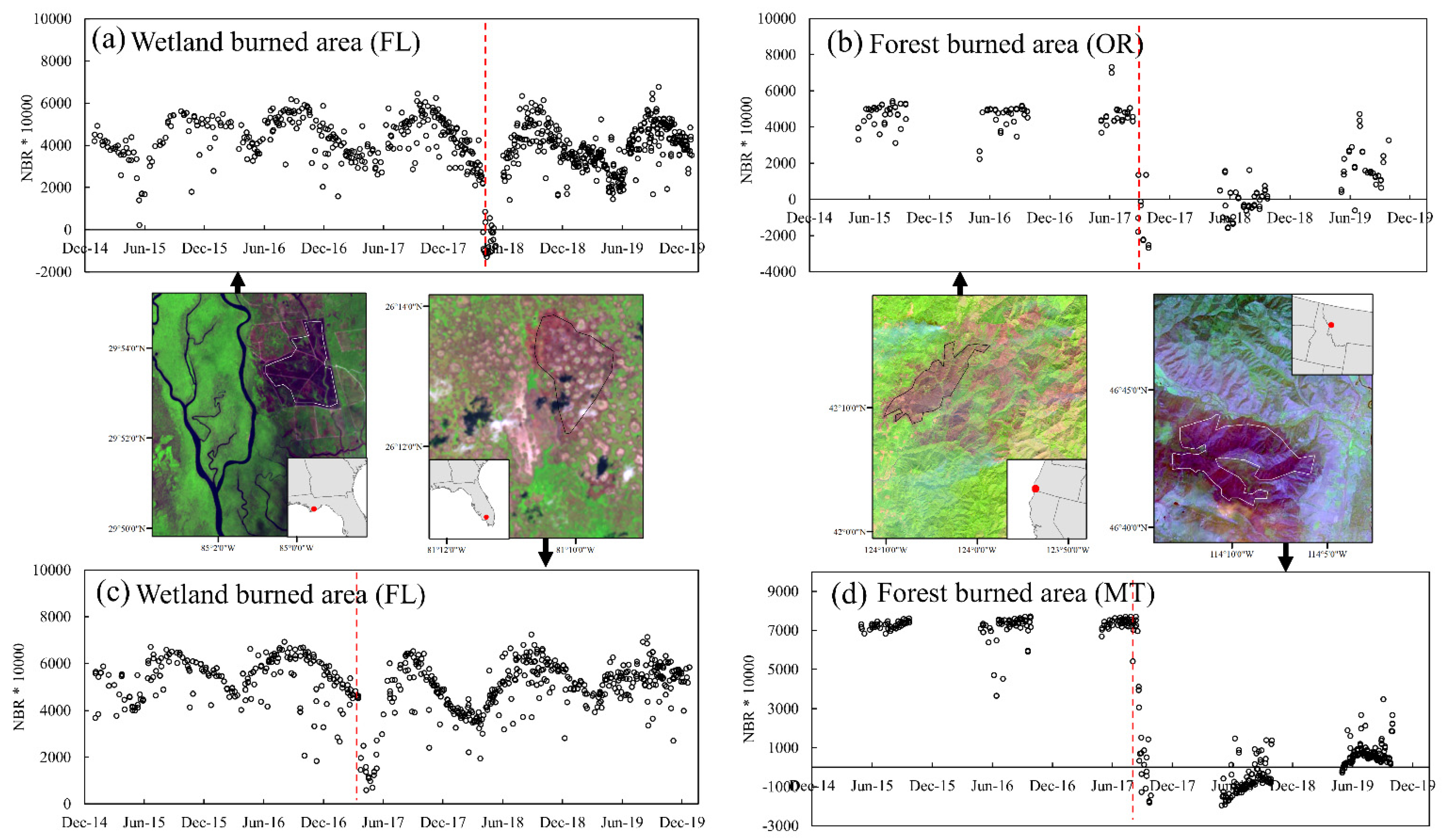
38]. The probability of mapping wetland fires will depend in part on the persistence of the burn signal, which can be much shorter for wetlands relative to upland forests, and shorter for wet and warm southeastern ecosystems, relative to drier western ecosystems (Figure 1). In wetlands, the persistence of the burn signal is influenced by the season in which the fire occurs [25,39], as well as the burn severity and site wetness [12], but is often negligible one-to-three months post-fire [11,32,39]. These challenges demonstrate the need for new approaches to improve our understanding of burned-area extent in wetland ecosystems.
Sentinel-2 satellites (2A launched 23 June 2015 and 2B launched 7 March 2017) can provide clear-sky imagery, in complement with imagery collected by Landsat-8, to meet these wetland-specific challenges across the Southeast. In addition, Sentinel-2 imagery maintains a moderate spatial resolution (10–20 m), relative to existing global burned area products (≥250 m) [40]. While global products, such as MCD45, are derived from near-daily imagery, the coarse spatial resolution (500 m) produces a high omission error in temperate ecoregions, with documented omission errors of 87% in temperate grassland and savanna and 99% in temperate forest [41]. Global burned area products have not been explicitly validated in wetland ecosystem types [41]. In recent years, approaches to track burned area have emerged by using Sentinel-2 alone [42,43,44] or using both Landsat-8 and Sentinel-2 [45,46,47]. However, the Sentinel-2 efforts to date have focused on a subset of land-cover types, using Sentinel-2 to track burned area across African savannah ecosystems [42,45,48] and forests [44,46].
The timing of wetland fire ignitions across the Southeastern US is driven by the climate conditions and the cause of the fire. Climate has a strong influence on wildfires by controlling the fuel quantity and moisture, fuel connectivity, and lightning ignition potential [49]. Drier and warmer conditions increase the total wetland area burned [36,50]. However, humans also play a strong role in the timing and cause of fires [51]. For example, unlike wildfires, prescribed fires tend to be set during wetter conditions [11], so that prescribed fires extend the fire season beyond what would otherwise occur. Most wildfires across southeastern wetlands occur during the early growing season (April/May) near the end of the dry season when fuels are dry, ground water levels are low and lightning frequency is relatively high, while prescribed fires are typically closer to the beginning of the dry season (January/February) [10,52,53].
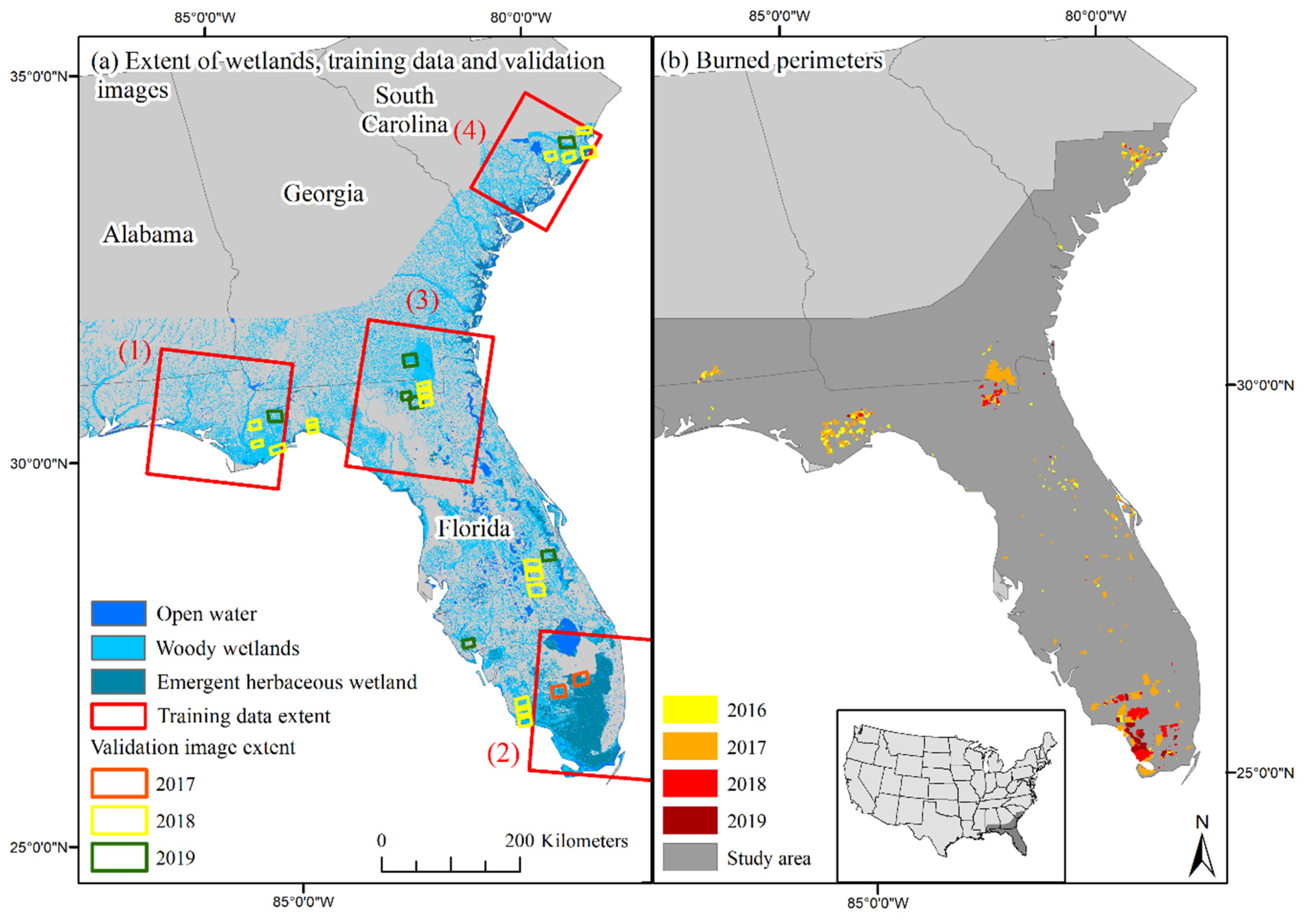
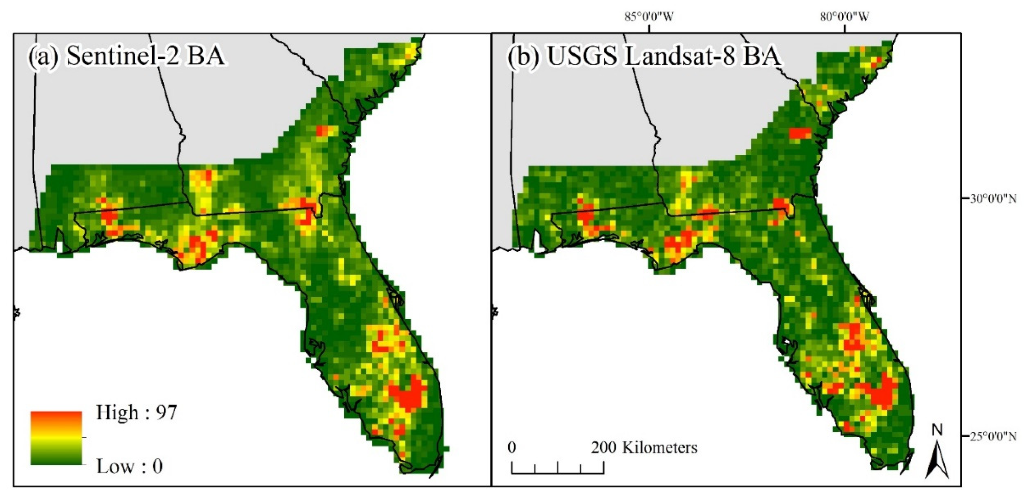
In this study, we developed an algorithm to map the burned area extent in wetland ecosystems by using the Sentinel-2 image archive across Florida and the coastal portions of Alabama, Georgia, and South Carolina. The USGS Landsat BA [
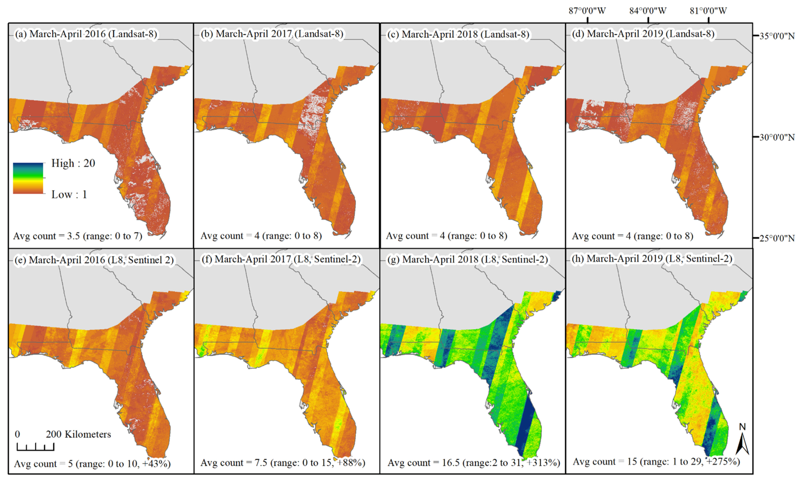
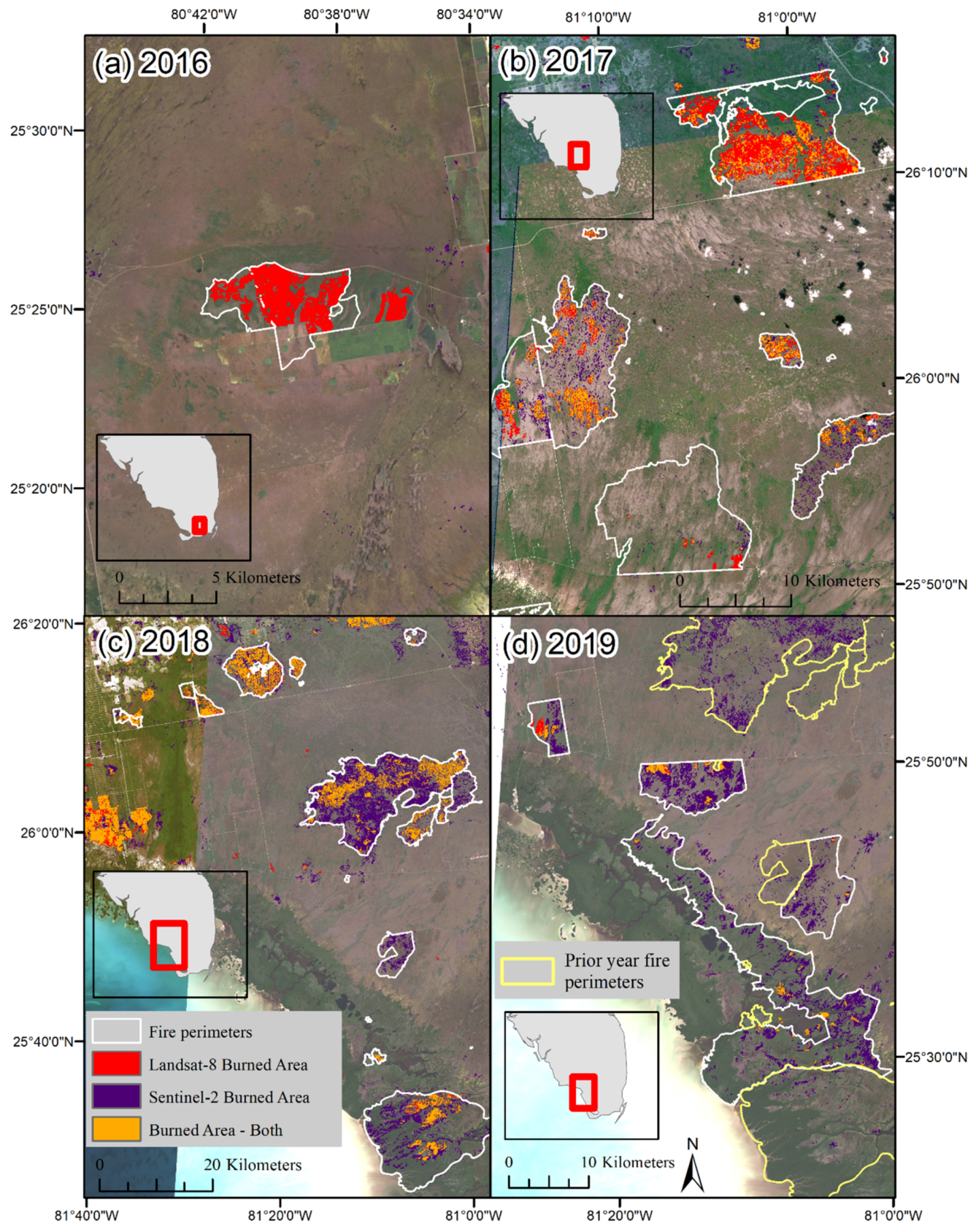
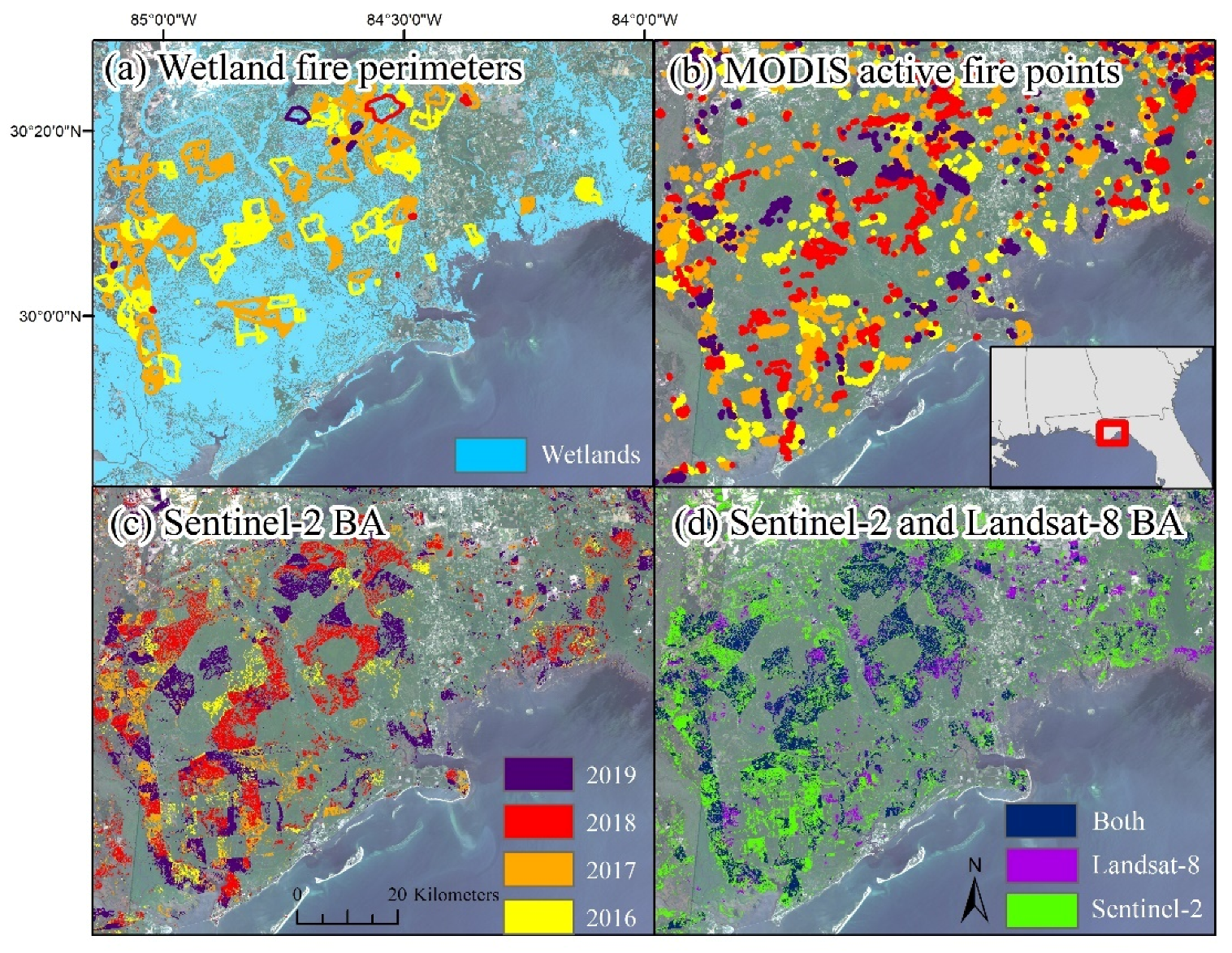
34] is currently the finest resolution burned area product operationally produced across the US. However, Landsat-7 is 22 years into its mission and is likely to be de-commissioned soon. It is critical, therefore, to explore the extent to which Sentinel-2 may supplement the Landsat-8 (L8) BA, particularly in regions with rapid regrowth such as the Southeastern US. To do so, we addressed the following research questions: (1) What is the contribution of clear-sky observations from Sentinel-2, relative to Landsat-8? (2) Can Sentinel-2 effectively map burned areas in wetland ecosystems? (3) What are the individual and combined contributions of Sentinel-2 and Landsat-8 to burned area extent in wetlands, and how do they compare to verified wetland fire perimeters?

2. Materials and Methods

2.1. Study Area

The study was focused on a subset of the Southeastern US, defined here as Florida, and the coastal portions of Georgia, South Carolina, and Alabama (up to 200 km from the coast, total area = 293,821 km2) (Figure 2). The region has a humid, subtropical climate. Annual precipitation averages 1315 mm, and annual temperature maximum and minimum average 26 and 14 °C, respectively [54]. Across the region, emergent and forested wetlands are the dominant land-cover type (32%, Figure 2a), followed by evergreen forests (22%) and agriculture (19%, cultivated crops, hay/pasture) [55]. Wetland extent within this study was defined by using the National Wetland Inventory (NWI, version 2.0) dataset. Wetland extent averaged 29 ha km−2 across the region with wetland area dominated by freshwater forested/shrub wetlands (50%), estuarine and marine wetlands (21%), and freshwater emergent wetlands (11%) [56].

2.2. Clear-Sky Contributions of Sentinel-2

Clear-sky observation counts were calculated in Google Earth Engine [57]. All Landsat-7 (non-gap filled) and 8 surface reflectance, and Sentinel-2 top-of-atmosphere images collected in 2016–2019 across the study area were used. Values identified as cloud or cloud shadow in Landsat-7 and Landsat-8 images were masked using cFMask [58]. Cloud and cloud shadow masks were applied to the Sentinel-2 image collection, as described in Section 2.3.1. The Normalized Difference Vegetation Index (NDVI) was calculated for all unmasked pixels across the three image collections. The per-pixel observation count of NDVI was summed annually and for March/April of each year (2016–2019). This two-month period represents the seasonal peak in fire activity [24]. For multisensor comparisons, the per-pixel observation count was summed across sensors. Because Landsat-7 is still active, contributing clear-sky observations from this sensor were also calculated for comparison purposes.

2.3. Burned Area Algorithm Development

For burned area, we trained and validated the algorithm entirely on burned pixels within wetlands identified by using the National Wetland Inventory dataset and limited to estuarine and marine wetlands, as well as freshwater emergent, shrub, and forested wetlands [56]. For unburned areas, we trained and validated the algorithm across both wetland and non-wetland land-cover types. Because wetlands often occur in a mosaic with other land cover types, fire events frequently extend beyond a wetland boundary. To avoid mapping only parts of fire events, the burned area algorithm was applied across the entire study area.

2.3.1. Image Collection Preprocessing

All Sentinel-2 top-of-atmosphere (TOA) image collection (Level 1C) images acquired within the study area between 1 January 1 2016, and 31 December 31 2019, were processed. To mask clouds, we used the Sentinel-2 cloud probability layer [59], where pixels with a probability of >50% were classified as clouds and were masked out. Because the Level 1C image collection lacks a cloud shadow mask, cloud shadows were identified and masked by modifying code provided through the Google Earth Engine Community, “Sentinel-2 Cloud Masking with s2cloudless”. Cloud shadows were defined as the intersection of the predicted cloud shadow area, derived from the cloud probability layer and the mean solar azimuth angle, and dark areas, identified as low-reflectance, near-infrared (NIR) pixels. To compensate for potential atmospheric contamination, we avoided using single spectral bands as variables and instead relied on normalized spectral indices. Google Earth Engine sets image count limits to control memory use. As Sentinel-2 is delivered as tiles, image stacks can rapidly exceed memory limits. Consequently, all images collected on the same date were mosaicked into a single image to reduce image counts.

2.3.2. Training Data

Training pixels were sampled from Sentinel-2 training images selected to represent four subregions across the Southeast that experience high amounts of wetland fire: (1) the Florida panhandle, (2) the Florida Everglades, (3) the coastal plains of South Carolina, and (4) the Eastern Florida–Georgia border (Figure 2). In each training image, burned points were randomly sampled within burn perimeters mapped by or created from (1) the Geospatial Multi-Agency Coordination (GeoMAC) [60], now National Incident Fire Services (NIFS), (2) the Wildland Fire Decision Support System (USGS WFDSS, https://wfdss.usgs.gov/wfdss/WFDSS_Data.shtml (accessed on 12 May 2021), or (3) clusters of points identified by the MODIS Active Fire Product (MCD14) [20]. All burned points were restricted to palustrine emergent, palustrine forested/scrub–shrub, or estuarine and marine wetlands, as defined by the NWI dataset, and were checked to ensure that the burned signal was visually observable in the training image. Unburned points were randomly selected outside the burn perimeters to represent all unburned conditions (e.g., unburned wetland, forest, urban, grassland, and agriculture). In each of the four regions, we selected 400 burned training points and 400 unburned training points spread across six images representing seasonal variability (two December–February images, two March–May images, one June–August image, and one September–November image). The one exception was South Carolina, where an extra spring image was added to increase the number of images with burned points present. A total of 3200 training points across 25 images were generated. All training images, as well as the number of burned points per image, are shown in Appendix A Table A1. The variable values for the pixel corresponding to each training point were extracted and used to train the burned area algorithm.

2.3.3. Variables Considered

Spectral indices that have been shown to be helpful in identifying burned area were considered as potential variables and are listed in Table 1 [34]. Because Sentinel-2 lacks thermal bands, indices that included thermal bands were excluded from consideration. Single spectral bands (i.e., blue, red, and NIR) were also excluded from consideration, because we found that random forest models fit to the training data with single bands tended to show higher rates of error when applied to the imagery time series. For each of the 14 spectral indices, we considered the (1) single scene variable, (2) z-score value of the variable, and (3) monthly change value of the variable (14 spectral indices × 3 versions = 42 variables). The z-score values were calculated by subtracting the per-pixel mean and dividing by the per-pixel standard deviation over the time series. Monthly mean values for each predictor were calculated, and change from the monthly mean was calculated by subtracting the specific monthly mean over the time series from the pixel value. To account for potential spectral confusion between increases in wetland water level and burned areas, we also included two Standardized Precipitation Index (SPI) [61] variables, where precipitation was aggregated for the last 30 days (spi30d) and 90 days (spi90d), respectively, relative to the date of the image acquisition. The data were derived from 4 km daily Gridded Surface Meteorological (GRIDMET) data [62]. The precipitation data were standardized relative to 1981–2016, assuming an inverse-normal distribution. The 42 spectral variables combined with the two precipitation variables produced a total of 44 variables that were considered for inclusion in the model. The values of each of the variables for all training points were extracted and exported from Google Earth Engine.

2.3.4. Model Variable Selection and Application

We used the Python package, geemap to access, analyze, and visualize the Sentinel-2 image collection, as well as the GRIDMET data, in the Jupyter environment [77]. Random forest classifiers were fit using the Scikit-learn Python module [78]. We sequentially tested the suite of potential predictors and, in each step, selected the predictor that increased the Random Forest’s Area Under the Curve (AUC) the most. In each step, predictors were removed if they had high correlation (≥0.95) with any of the selected predictors. Predictors were selected until the increase in AUC of additional variables was <0.0001. We also evaluated how model accuracy changed with the number of training points to ensure our sample size was sufficient (100 iterations, 20% randomly selected each time as validation set). The selected predictor variables were then used to train a final Random Forest model, using Scikit-learn in a Jupyter Notebook environment (https://jupyter.org/, accessed on 12 May 2021), accessed through Miniconda 3 (https://docs.conda.io/en/latest/miniconda.html, accessed on 12 May 2021). We ran 300 trees with bootstrapping. The trees were translated into text and compiled into a list of trees readable to Google Earth Engine, using the ee.Classifier.decisionTreeEnsemble method, and applied to all Sentinel-2 images. Variable importance was calculated with Python Scikit-learn as the permutation importance, which reports the mean decrease in accuracy.
Temporary turbidity in open water was a source of commission error and was masked out by identifying permanent open water. Long-term (2016–2019) open water was defined as having a median Normalized Difference Wetness Index (NDWI, normalized difference of green and NIR bands) value of >0.14, where water values tended to be positive and land values tended to be negative. This threshold was selected by iteratively testing threshold performance across the study area to mask out open water bodies but avoid masking out wetlands. During the study period, this region experienced two category 5 hurricanes: Hurricane Irma made landfall on 10 September 2017 and traveled up the western coast of Florida, and Hurricane Michael made landfall on the Florida panhandle on 10 October 2018. Hurricanes of this magnitude cause substantial flooding and damage; therefore, Sentinel-2 images for the Florida panhandle were excluded between October and December 2018, and Sentinel-2 images within the Everglades and the western coast of Florida were excluded between October and December 2017 to reduce post-hurricane commission error. Both hurricanes showed extended impacts, however, into the following spring, primarily along riparian corridors in the path of the hurricane. To reduce riparian commission error along the path of the hurricane, a pixel was masked out if the normalized difference of the NIR and coastal bands averaged between −0.05 and 0.25 across December, January, and February in the winter following each hurricane. This value range and months maximized distinguishing documented burned area from hurricane-related impacts. In addition, very limited manual editing was performed, but only after the validation analysis was complete. In this step, the direct paths of Hurricane Irma and Hurricane Michael were reviewed for false positives in the spring following each hurricane.
For each year, the classified Sentinel-2 images were consolidated into the burn count for January–May and the burn count for June–December. Because both wildfires and prescribed fires were most common in the January–April period, burn counts of 2 or more were reclassified as burned for this 6-month period. In contrast, burn counts of 3 or more were reclassified as burned for the June–December burn count raster in each year. This enabled us to limit the inclusion of TOA images with a lower than average signal to noise ratio. To reduce commission error, only burned polygons >1 ha were retained. Finally, the spring and fall burned areas were combined to produce an annual raster that was filtered by using a 5 × 5 bit error adaptive filter to reduce noise while preserving edges [79].

2.4. Validation

We evaluated the Sentinel-2 burned area classification by using validation points (burned and unburned) derived from WorldView-2 and WorldView-3 images (Figure 2a). Worldview-2 (2 m resolution) and Worldview-3 (1.4 m resolution) images (n = 27) were selected by using disproportionate sampling [80,81] to ensure that enough wetland burned area was considered in the validation (Appendix A Table A2). The image acquisition dates ranged from 26 February 2017 to 6 December 2019. The images were acquired via the NextView License as Level 2A 8-band images. Within each high-resolution image, burned area that occurred within or overlapped wetlands, as defined by the NWI dataset, was manually delineated as (1) visually distinguishable from the high-resolution imagery and (2) verified as a burned area by a secondary source, specifically MODIS active fire points [20] or historical high-resolution imagery available in Google Earth Pro, for burns missed by the MODIS active fire dataset. A total of 319.8 km2 of burned area across 54 fires, within or overlapping wetlands was delineated, which represented 5.3% of the non-overlapping high-resolution image extent. We then randomly generated validation points with the class proportionate to the amount of burned area cover (5%), so that 1000 points were randomly selected within the burned perimeters and 20,000 points were randomly selected outside the burned perimeters. Each point was visually checked to ensure the accuracy of the assigned class and points were reassigned as needed. The creation of the validation dataset was completed independent of the Landsat BA and the Sentinel-2 burned area produced in this analysis. Points used to train the algorithm did not overlap with points used to validate outputs. For the validation points associated with each high-resolution image, the nearest date, relatively cloud-free Sentinel-2 image was processed to burned/unburned and used to evaluate the Sentinel-2 burned area (Appendix A Table A2). For comparison, we also validated the L8 BA, using the same set of validation points (Appendix A Table A2). Because of variable timing in the fire activity relative to the image collection, the Sentinel-2 and L8 BA images selected for validation were not necessarily the closest date match, but instead, the single image that best mapped the burned area. This decision was made because the nearest date image sometimes had substantial cloud cover. In addition, this approach helped avoid cases in which a burned area was visible in a high-resolution image, but the fire event had not yet occurred in a Sentinel-2 or L8 image collected several days prior. NA values within the selected images were excluded from inclusion in the accuracy statistics.
Omission (OE) and commission (CE) errors were calculated for the “burned” category [82]. The Dice coefficient was calculated as the conditional probability, presented as a percentage, that if one classifier (product or reference data) identifies a pixel as burned, the other one will as well, integrating omission and commission errors [83,84]. The relative bias was also calculated, providing the proportion, presented as a percentage, that burned area is under or overestimated relative to the total burned area of the reference product [41]. To account for the influence of validation points being clustered within each high-resolution image, standard errors were calculated by using the stratified combined ratio estimator [85,86]. Using the numerator and denominator of the accuracy metric for the set of validation points associated with each high-resolution image individually, this approach calculated the variance and standard error of each regional accuracy metric (survey R package) [87].

2.5. Analysis

The potential contribution of the Sentinel-2 burned area was evaluated by comparing the annual Sentinel-2 burn area raster to wetland burn perimeters compiled from multiple fire databases (Figure 2b). All burn perimeters were compiled from datasets where they were verified manually. Sources of burn perimeters included (1) the Monitoring Trends in Burn Severity (MTBS) [88], (2) GeoMAC, (3) WFDSS, and (4) perimeter datasets including prescribed fires compiled from the US Forest Service, National Park Service, the Florida Forest Service, and the Nature Conservancy. The burned perimeters were required to overlap an NWI polygon, and burn perimeters < 1 ha were excluded to match the minimum unit size of the Sentinel-2 burned area. A total of 555 wetland fire perimeters were included across the study area, totaling almost 537,000 ha over the four-year period. The Sentinel-2 burned area, the L8 BA, and the combined burned area, all compiled as annual composites, were compared to the wetland burned polygons and evaluated for detection count, defined as the number of burn perimeters that showed an overlap between the burn perimeter and burned area, as well as the total area of the burn perimeters classified as burned. Detection by wetland type and by burned area perimeter size were also evaluated. Wetland type was defined by the majority NWI wetland type within the burned perimeter [56]. For this analysis, wetland types were restricted to (1) freshwater (palustrine) forested and shrub wetland, freshwater (palustrine) emergent wetland, and estuarine and marine wetlands, while riverine, lake, and pond NWI wetland types were excluded.

3. Results

3.1. Sentinel-2 Clear-Sky Observation Contribution

Sentinel-2 can contribute to monitoring burned area by increasing the frequency of clear-sky observations across the Southeast. Adding Sentinel-2 observations to Landsat-8 observations in the peak fire period, March/April, increased the observation count between 43% in 2016 and 313% in 2018 across the study area (Figure 3). On an annual time-step, adding Sentinel-2 to Landsat-8 in 2016 increased observation count from 17 to 46. With the launch of Sentinel-2B in 2017, the observation count increased from 16 with Landsat-8 alone to 78 by 2019 (Table 2). The increase in Sentinel-2 observation count in 2018 and 2019 relative to 2016 and 2017 was evident not only in observation count (Table 2) but also the net contribution of burned area extent, relative to the L8 burned area extent. In Figure 4, for example, we observed a greater “new burned area” identified by Sentinel-2 in 2018 and 2019 across the Everglades, relative to 2016 and 2017.

3.2. Model Performance and Burned Area Validation

When the model score was related to the number of training points, by 1400 training points, we saw limited further improvements in model score, suggesting that the number of training points used in the development of the burned area random forest model was sufficient (Figure 5a). Out of the 44 potential independent variables tested, nine variables were selected for inclusion in the Sentinel-2 Random Forest model (Figure 5b). The z-score of the NIR-red ratio vegetation index (VI43) and the change from monthly mean of the shortwave infrared and NIR ratio (VI45) showed both high variable importance and the biggest contributions to the AUC. The change from monthly mean of the Enhanced Vegetation Index (EVI) also showed high variable importance but lower contribution to the AUC (Figure 5b). In total, one z-score variable, three change from monthly mean variables, three single scene variables, and both the 30- and 90-day SPI variables were all selected for inclusion in the Random Forest model (Figure 5). We tested the Spearman correlation values between the selected variables and found a maximum correlation of −0.85 between the change from monthly mean EVI and change from monthly mean NDWI. The average absolute correlation value between all of the selected variables was 0.37. The model’s AUC was 0.998, while the model’s cross-validation score was 0.92 (Figure 5).
Strong model fit metrics, however, do not necessarily indicate how well the model will perform when applied to a time series of imagery; additional validation is necessary. The absolute average date gap between Sentinel-2 and the high-resolution validation images was 7.0 days, while the absolute average date gap between the Landsat-8 images and the selected high-resolution images was 11.6 days (Appendix A Table A2). The L8 BA showed a 47 ± 5% and 8 ± 3% error of omission and commission for burned area, respectively (Table 3). Sentinel-2 burned area, in comparison, showed a lower error of omission (29 ± 7%) but a higher error of commission (30 ± 4%). However, the Dice coefficient (70 ± 5% relative to 67 ± 5%) and relative bias (2 ± 8% relative to −42 ± 4%) were both stronger in the Sentinel-2 burned area validation relative to the L8 BA validation (Table 3).

3.3. Burned Area Extent and Analysis of Burn Perimeter Detection

Burned area impacts a small proportion of land area annually; therefore, burned area products are often difficult to view at a regional scale. To improve visibility, the proportion of a moving window mapped as burned was generated to indicate the burned area patterns (Figure 6). Across the study area, the Sentinel-2 burned area showed a similar geographical burn pattern between 2016 and 2019 as the L8 BA Product (Figure 6). However, some differences were visible, for instance, the Sentinel-2 BA showed a higher proportion of burned area in Southwestern and Southeastern Georgia, while the Landsat-8 BA showed a higher proportion of burned area at the Southern Georgia border and Eastern Florida. Across the study area, averages of 2.1% and 1.1% of the NWI wetlands, defined as estuarine and marine wetlands, as well as freshwater emergent, shrub, and forested wetlands, were mapped as burned each year by Sentinel-2 and the L8 BA, respectively. In comparison, The Landsat Burned Area product mapped 0.4% of the conterminous US as burned each year, with 0.6% of CONUS mapped as burned in 2012, the highest fire year [34].
We compared the Sentinel-2 and L8 burned area to the wetland burn perimeter dataset (n = 555) to quantify the relative contribution of Sentinel-2 burned area. Sentinel-2 exceeded Landsat-8 in all four years in the percent of the wetland burn perimeters detected and in all years except 2016 for the percent of the wetland burn perimeters mapped as burned (Table 4). An example of this finding is shown in Figure 7, where Sentinel-2 identified additional burned area relative to the L8 BA, but showed a similar burn pattern as MODIS active fire points and the L8 BA across the Apalachicola National Forest in the Florida panhandle. Across the four-year period, by count the L8 BA detected 60% of the perimeters, while Sentinel-2 detected 79% of the perimeters and together 79% of the perimeters were detected (Table 4). Although burn perimeters are typically an overestimate of burned area and include unburned areas within the burn perimeter, mapping more area as burned suggests the detection of burned area across a larger range of burn severities. By area, the L8 BA detected 32% of the perimeter area compared to 39% detected by Sentinel-2, and together the two sensors mapped 50% of the perimeter area as burned (Table 4).
The detection of wetland burn perimeters by Sentinel-2 varied by wetland type and burn perimeter size. Burn perimeters overlapping palustrine forested or scrub–shrub wetlands represented 52% of the perimeters, while the remaining were split between palustrine emergent wetlands (26%) and estuarine and marine wetlands (22%). The Sentinel-2 burned area detected 97% of the palustrine forested or scrub–shrub wetland burn perimeters, compared to 74% of the palustrine emergent wetland burn perimeters, and only 37% of the estuarine and marine wetland burn perimeters (Table 5). An example of burned-area detection in South Carolina across an area dominated by forest/scrub–shrub wetlands shows that Sentinel-2 contributes burned area relative to not only L8 BA but also Landsat-7 BA (Figure 8). In addition to patterns by wetland type, we also observed a pattern by burn perimeter size. While only 40% of the perimeters between 1 and 10 ha were detected, 68% of the burn perimeters 11 to 20 ha were detected, and >97% of the burn perimeters 200–500 ha in size were detected (Table 5). Sentinel-2 burn polygons <1 ha in size were filtered out in postprocessing to reduce speckling, which reduced noise but likely increased omission of smaller (1–10 ha) burn perimeters.
Although the algorithm was trained using data points from four distinct wetland regions, the burned area algorithm was applied across the entire study area. Figure 9 shows examples of how the Sentinel-2 burned area algorithm performed, relative to the Landsat-8 burned area and the MODIS active fire points, outside of the areas in which it was trained, including mapping burned area in wetlands along Florida’s eastern coast (Figure 9a–c), and mapping burned area in forest and scrub/shrub land-cover types (Figure 9d–i).

4. Discussion

Fires in wetland ecosystems are common across the Southeastern US, as well as globally [11,12,52]; however, existing burned-area products underestimate wetland burned area [24,34], which contributes to error in accurately tracking changes in terrestrial carbon storage and carbon emissions [8,18]. In this effort, we used a machine learning algorithm, trained on wetland fires, to map burned area extent (2016–2019), using the Sentinel-2 archive across Florida, as well as parts of Alabama, Georgia, and South Carolina. Burned area in wetlands can go undetected when a burned area is visible but omitted by a burned area algorithm due to low burn severity, burnable wetlands being masked out, or an atypical burn signal [11,38]. Burned area in wetlands can also go undetected when the burned area was never visible during image collection dates because of rapid vegetation recovery and cloud cover [25,26]. The finer spatial resolution and greater frequency of the Sentinel-2 imagery collection can help improve estimates of carbon emissions [89] from wetland fires. With the imminent decommissioning of Landsat-7, and Landsat-9 not yet launched or operational, Sentinel-2 or the harmonized Landsat and Sentinel-2 dataset [90] can potentially be used at a national scale to enhance the USGS BA Product. By training the algorithm using burned area in wetlands only and designing the open water mask to avoid masking burnable wetlands to the extent possible, we demonstrated that Sentinel-2 can be effectively used to support regional-scale efforts to find and track wetland burned area. Additionally, modifying the algorithm to include wetland burned area in other burnable wetland types, such as peat bogs, could improve the model transferability to other regions where wetland fires are common.
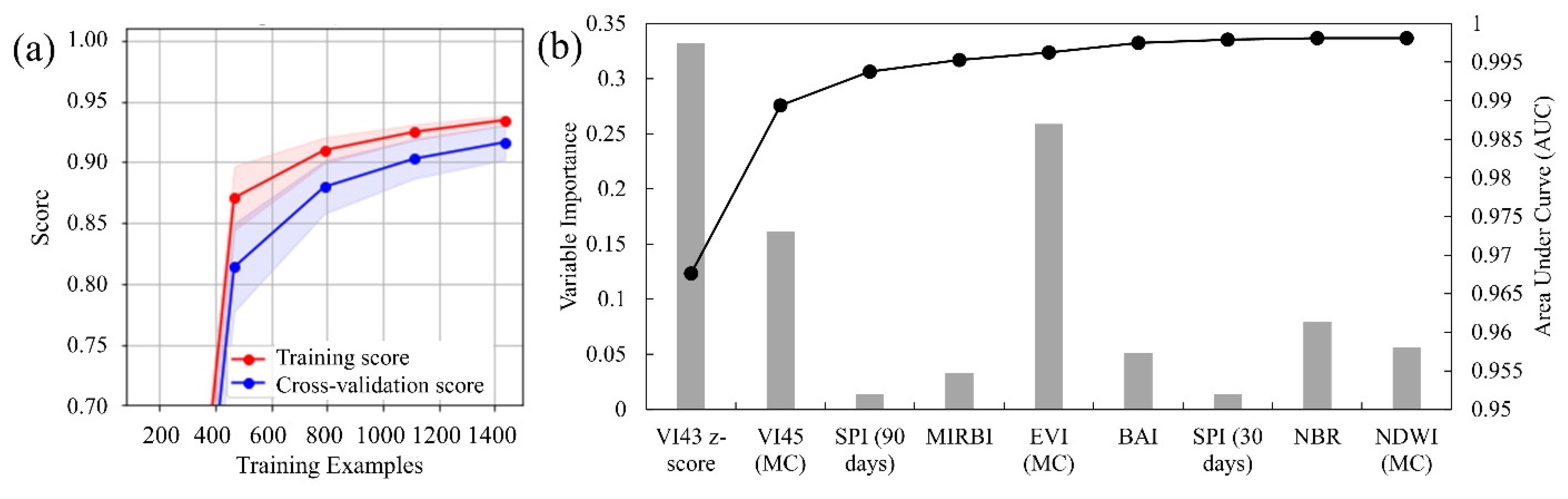
Assessment of algorithm accuracy is a critical component of burned area algorithms. The accuracy of our Sentinel-2 burned area (29% OE, 30% CE) was similar to other efforts that used Sentinel-2 to track burned area, for instance, a 33% OE and 31% CE from mapping fires with Sentinel-2 across Tropical and Subtropical African savannah sites [48], and a 27% OE and 19% CE mapping fires from Sentinel-2 across Sub-Saharan Africa [42]. However, in converting from single-image classification, on which our validation was performed, to annual composites of burned area, we observed that a small percentage of images in the time series introduced a disproportionate amount of error. To remove potentially problematic images, we used a seasonally specific burn count threshold. This step, while reducing commission error in the annual mosaic, also contradicted our original argument that observation count is key to wetland fire detection [11,12,25]. An alternative approach is to threshold and segment burn area from predicted burn probability surfaces instead of using burn count [27,34]. Using burn probability instead of burn count potentially retains burned areas that are only visible in a single image. However, when testing this approach in the algorithm development stage, we found that this approach also missed documented burns. This source of error highlights the challenge of minimizing commission error in algorithms applied to dense stacks of imagery, while also minimizing omission error when the burn signal is often subtle in wetland ecosystems. While additional preprocessing, such as conversion to surface reflectance, could potentially reduce noise, other efforts have shown that surface reflectance does not necessarily outperform TOA imagery in wetland and water environments [91,92]. Alternative approaches to identify and remove images with a lower-than-average signal-to-noise ratio may therefore be necessary [93].
Relative to other land-cover types, wetlands show both a high diversity in vegetation type and structure, and a high amount of temporal variability, attributes that make it especially challenging to distinguish burned area extent. This challenge is made more difficult because water and burned area show substantial overlap in their spectral reflectance [21,30,31]. Forested wetlands are abundant across the study area but can be difficult to discern, as they occur under the forest canopy. Water levels in this wetland type respond not only to variability in precipitation, but also typically show an inverse relationship with leaf-cover and leaf-out attributable to tree evapotranspiration [94]. Tidal, emergent wetlands are typically vegetated with salt-tolerant species that change with height above sea level, and experience constant tidally induced changes in water level [1]. Freshwater emergent wetlands, in contrast, primarily respond to variability in precipitation, but wetland vegetation types, such as cattails, bulrushes, saw grass, and maidencane, differ in height and structure from other types of wetland vegetation, such as bladderworts and water lilies, which can float on the water’s surface [
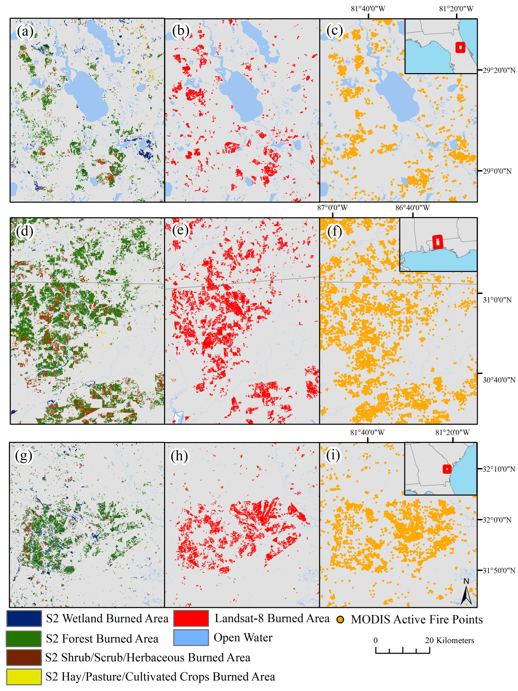
1]. These differences, which are attributable to wetland type, may be why we found that the Sentinel-2 burned area performed unevenly across different wetland types. For example, while most palustrine forested or scrub–shrub wetland burn perimeters were detected, less than 40% of the estuarine or marine wetland burn perimeters were detected (Table 5). This finding suggests that algorithms focused on wetland areas need to be sensitive to post-burn changes in spectral reflectance that are not typical for other vegetation types (e.g., forests). For example, wetland vegetation can burn off during a fire event, leaving open water, and a fire event can also initiate a rapid burst of vegetation growth leaving the area temporarily greener than nearby unburned areas [32,35]. In the algorithm development stage, we found that these types of post-fire transitions did not represent most wetland fires. However, consideration of non-traditional changes (e.g., to open water or greener) may need to be considered in future efforts to map a more complete record of wetland burned areas. Doing so requires spatially coincident information about land-cover and vegetation types, as well as expected timing in water level and phenology.
Algorithms also need to be sensitive to lower burn severity, which is often associated with prescribed burns [21,28,29]. Explicitly training algorithms on both prescribed fires and wildfires can help improve an algorithm’s performance, which we saw, by the Sentinel-2 burned area identifying more area of the perimeter dataset as burned, relative to the Landsat-8 BA. However, mapping prescribed fires as distinct from wildfires will require relating remotely sensed BA products to prescribed fire records and datasets [51], which remains challenging [27].
Wetlands are dynamic systems that experience structural changes from seasonal shifts in water level, episodic fire events, and, in the Southeastern US, tropical storms and hurricanes. In this effort hurricane related flooding and vegetation damage was a substantial source of error. For instance, we observed an increase in commission error in wetlands along the southern and western edge of the Everglades starting in September 2017 with the timing of the error coinciding with the landfall of Hurricane Irma on September 10, 2017 that caused substantial flooding and sediment movement as it traveled up the western coast of the Everglades [95]. When we tracked wetlands misclassified as burned, we found a shift in the spectral signature that persisted from September 2017 until February 2018. In contrast, because the area where Hurricane Michael made landfall was dominated by forest, the region experienced substantial blow-down [96], meaning that the damage persisted for a longer period post-hurricane relative to Hurricane Irma. In both cases, we observed an increase in commission error that was most prominent along riparian corridors. The hurricanes complicated efforts to accurately map burned areas near where the hurricane made land fall; however, we saw a rapid reduction in commission error as the hurricanes moved farther inland. In response to this source of error, we removed imagery at the site where each hurricane made landfall for the October–December post-hurricane period and implemented a temporary riparian mask for December–February to further reduce hurricane-related error. However, sustained impacts from the hurricane remained a source of error for the burned area mapping effort. Specifically training the algorithm on storm damage and impacts may help reduce this type of error.
Increasingly, cubesats and other commercial satellites are collecting multispectral imagery that may have potential applications for mapping burned area [97,98]. However, often these satellites are restricted to visible and NIR bands, which enable algorithms to detect changes in greenness [63,70], but prevent the calculation of some of the most common burn related indices, such as the Normalized Burn Ratio (NBR), which requires shortwave infrared bands [66,67]. In wetlands, using satellites that provide shortwave infrared bands may be especially important. As water levels rise in vegetated wetlands, the spectral reflectance in the NIR declines [38], meaning that saturated wetlands can look very similar to burned areas. Even NBR, however, tends to perform less consistently in unforested areas [73], where the index may respond more to soil wetness than plant coverage [12]. Using Landsat satellites, indices that incorporated the thermal band were found to reduce confusion [34,38]. For sensors that lack the thermal band, such as Sentinel-2, we demonstrated that ancillary sources of data, such as GRIDMET standardized precipitation index can potentially help the algorithm identify when darker-than-normal ground conditions may be attributed to an increase in wetness instead of a burn event. Using precipitation data can also potentially support efforts to identify burned areas where vegetation burned off, revealing open water underneath. However, precipitation datasets, such as GRIDMET, are typically coarse in resolution (4 km), while one of the advantages to using Sentinel-2 is its moderate spatial resolution (20 m) relative to existing global burned area products (≥500 m). Alternatively, it is possible that using a synthetic aperture radar (SAR) satellite, such as Sentinel-1, to estimate changes to water level, or a Sentinel-2 or Landsat-based estimate of inundation extent, could serve a similar role in helping distinguish an increase in wetness from a burn event or when a change from vegetated to non-vegetated water may be attributable to a burn event instead of a rise in water level. As Sentinel-1 now provides regularly collected imagery, opportunities exist to develop burned area algorithms from SAR sensors [48,99]. Although the algorithms, to date, have tended to underperform relative to Sentinel-2 [48], SAR sensors, such as Sentinel-1, have the added benefit of not being sensitive to cloud cover or smoke and therefore would provide many more viable images for burned area mapping across the frequently cloudy Southeast, and can potentially help support efforts to monitor burned area and track disturbance-related changes in wetland biomass [100].

5. Conclusions

This analysis represented the largest-scale effort to date, of which we are aware, to specifically find and map wetland burned area. We demonstrated that Sentinel-2 can be effectively used to map the wetland burned area, particularly from 2018 onward, as the high count of clear-sky Sentinel-2 observations provide an improved chance of detecting burned areas prior to wetland vegetation recovery. The algorithm performed particularly well in forested and scrub/shrub wetlands. However, greater attention to nontraditional burn trajectories (e.g., conversion to open water and enhanced greenness relative to unburned areas) will be essential to further improve the detection of wetland burned area, particularly in tidally influenced estuarine and marine wetlands, where the water level changes hourly, not just seasonally. While using ancillary datasets, such as precipitation, helped distinguish wet conditions from burn conditions, the challenge of distinguishing these two spectrally similar conditions remains, particularly in tidal wetlands. Wetlands, globally, store a disproportionate amount of soil carbon. This carbon storage is vulnerable to loss during wetland fire events, yet fires in wetlands remain understudied and under-mapped. Algorithms, similar to the one developed here, can be adapted for diverse wetland types across the globe and employed to provide more complete burned-area datasets within wetland ecosystems. An improved understanding of wetland fire occurrence, frequency, and extent is critical for the effective management of wetland fuel loads, carbon storage, and wildlife habitat.

Author Contributions

Conceptualization, M.K.V., T.J.H., C.T., J.N. and J.P.; methodology, M.K.V. and T.J.H.; software, M.K.V.; validation, M.K.V., A.K. and C.T.; formal analysis, M.K.V.; data curation, M.K.V., C.T. and A.K.; writing—original draft preparation, M.K.V.; writing—review and editing, M.K.V., T.J.H., C.T., J.N., J.P. and A.K.; visualization, M.K.V.; funding acquisition, M.K.V. All authors have read and agreed to the published version of the manuscript.

Funding

Funding to support this research was provided by the US Geological Survey’s Land Change Science Program and Center for Data Integration within the Core Science Systems Mission Area.

Acknowledgments

Thank you to Yen Ju Beal for her technical support of the project and Michelle Field for early explorations of this area of research through the National Association of Geoscience Teachers (NAGT) Program. Thank you also to Lara Douglas, Harland Goldstein, and the anonymous reviewers for their comments on earlier versions of the manuscript. Digital Globe imagery was made available via the Next View License. Data associated with this publication are provided through USGS’s Science Base upon publication (https://www.sciencebase.gov/catalog/item/603d2d6ed34eb1203117ef8f, https://doi.org/10.5066/P9S8SLEM, all accessed on 12 May 2021).

Disclaimer

Any use of trade, product, or firm names is for descriptive purposes only and does not imply endorsement by the US Government.

Conflicts of Interest

The authors declare no conflict of interest. The funders had no role in the design of the study; in the collection, analyses, or interpretation of data; in the writing of the manuscript; or in the decision to publish the results.

Appendix A

Table A1. Sentinel-2 images selected for training and the number of burned points randomly selected across each image. In each image 67 points were selected to represent unburned, except for the South Carolina training images, where 57 unburned points were selected per image to account for the inclusion of an extra training image. FL = Florida, GA = Georgia, N. = north, S. = south.
RegionSentinel-2 TileSentinel-2 DateBurned (Count)Total (Count)
Everglades17RNJ25 February 2017067
Everglades17RMJ17 March 2017182249
Everglades17RMJ25 November 2017067
Everglades17RMJ19 April 2018158225
Everglades17RNJ9 August 20181582
Everglades17RNJ17 December 201845112
FL Panhandle16RGU2 May 2017154221
FL Panhandle16RFU16 November 2017067
FL Panhandle16RFU30 January 201852119
FL Panhandle16RGV3 March 201887154
FL Panhandle16RFU23 August 2018067
FL Panhandle16RGU18 December 2019108175
N. FL/S. GA17RLP2 May 2017169236
N. FL/S. GA17RLQ3 November 2017067
N. FL/S. GA17RMP19 January 2018067
N. FL/S. GA17RLP17 April 2018169236
N. FL/S. GA17RLP8 July 201962129
N. FL/S. GA17RLQ18 December 2019067
South Carolina17SPS29 January 2017057
South Carolina17SPS9 May 2017158215
South Carolina17SPS29 April 2018145202
South Carolina17SNS28 July 2018057
South Carolina17SPS4 April 201997154
South Carolina17SPS11 October 2019057
South Carolina17SNS5 December 2019057
Table A2. Worldview-2 (WV2) and Worldview-3 (WV3) images used for validation. ARD = Analysis Ready Data, h = horizontal, v = vertical, FL = Florida, SC = South Carolina, GA = Georgia, L8 = Landsat-8.
SensorAcquisition DateImage NumberState (Region)L8 ARD TileL8 Image DateL8 Date GapSentinel-2 TileSentinel-2 Image DateSentinel-2 Date Gap
WV226 February 20173FL (south)h27v1811 February 2017−15T17RMK25 February 2017−1
WV226 February 20174FL (south)h27v1827 February 20171T17RNK25 February 2017−1
WV315 February 201812FL (north)h25v1628 February 201813T17RLP18 February 2018, 21 February 20183, 6
WV315 February 201810FL (north)h25v1628 February 201813T17RLP18 February 2018, 21 February 20183, 6
WV315 February 20189FL (north)h25v1628 February 201813T17RLP21 February 20186
WV213 March 20181SCh27v139 March 2018−4T17SPS22 March 20189
WV213 March 20184SCh27v139 March 2018, 3 April 2018−4, 21T17SPT22 March 20189
WV231 March 20182FL (panhandle)h24v1623 March 2018−8T16RGU17 April 201817
WV31 April 201822FL (panhandle)h24v167 March 2018−25T16RGU17 April 201816
WV31 April 201821FL (panhandle)h24v167 March 2018−25T16RGU17 April 201816
WV36 April 20182SCh27v139 March 2018−28T17SNS14 April 20188
WV36 April 20183SCh27v139 March 2018−28T17SPS15 March 2018−22
WV228 April 201810FL (south)h26v1910 April 2018, 26 April 2018−2, −18T17RMJ19 April 2018−9
WV228 April 20189FL (south)h26v1910 April 2018, 26 April 2018−2, −18T17RMK19 April 2018−9
WV228 April 20188FL (south)h26v1910 April 2018, 26 April 2018−2, −18T17RMK19 April 2018−9
WV33 May 201816FL (panhandle)h24v1624 April 2018−9T16RFU7 May 20184
WV33 May 201812FL (panhandle)h24v1624 April 2018−9T16RFU7 May 20184
WV219 June 20184FL centralh26v1729 June 201810T17RML28 June 20189
WV219 June 20182FL centralh26v1729 June 201810T17RML28 June 20189
WV219 June 20181FL centralh26v1729 June 201810T17RML28 June 20189
WV29 January 20197SCh27v137 January 2019−2T17SPS9 January 20190
WV312 March 201910FL (north)h25v1628 March 2019, 4 April 201916, 23T17RLP8 March 2019−4
WV226 March 201912FL centralh27v1728 March 20192T17RNM25 March 2019−1
WV222 April 20192GAh25v1520 April 2019−2T17RLQ22 April 20190
WV222 April 20197FL (north)h25v164 April 2019−18T17RLP22 April 20190
WV210 October 20191FL (panhandle)h24v164 October 2019−6T16RGU9 October 2019−1
WV36 December 201914FL (south)h26v189 December 20193T17RLL30 November 2019−6

References

  1. Federal Geographic Data Committee. Classification of Wetlands and Deepwater Habitats of the United States, FGDC-STD-004–2013, 2nd ed.; Wetlands Subcommittee, Federal Geographic Data Committee; U.S. Fish and Wildlife Service: Washington, DC, USA, 2013.
  2. Janse, J.H.; van Dam, A.A.; Hes, E.M.A.; de Klein, J.J.M.; Finlayson, C.M.; Janssen, A.B.G.; van Wijk, D.; Mooij, W.M.; Verhoeven, J.T.A. Towards a global model for wetlands ecosystem services. Curr. Opin. Environ. Sustain. 2019, 36, 11–19. [Google Scholar] [CrossRef]
  3. Mitra, S.; Wassmann, R.; Vlek, P.L. An appraisal of global wetland area and its organic carbon stock. Curr. Sci. 2005, 88, 25–35. [Google Scholar]
  4. Ma, A.-N.; Lu, J.-J. The progress of research on carbon flux in wetland ecosystems. Wetl. Sci. 2008, 6, 116–123. [Google Scholar]
  5. Ceballos, D.; Frangi, J.; Jobbágy, E. Soil volume and carbon storage shifts in drained and afforested wetlands of the Paraná River Delta. Biogeochemistry 2013, 112, 359–372. [Google Scholar] [CrossRef]
  6. Mitsch, W.J.; Bernal, B.; Nahlik, A.M.; Mander, U.; Zhang, L.; Anderson, C.J.; Jorgensen, S.E.; Brix, H. Wetlands, carbon, and climate change. Landsc. Ecol. 2013, 28, 583–597. [Google Scholar] [CrossRef]
  7. Lehner, B.; Doll, P. Development and validation of a global database of lakes, reservoirs and wetlands. J. Hydrol. 2004, 296, 1–22. [Google Scholar] [CrossRef]
  8. Mitsch, W.J.; Gosselink, J.G. Wetlands, 4th ed.; John Wiley & Sons, Inc.: Hoboken, NJ, USA, 2007. [Google Scholar]
  9. Nahlik, A.M.; Fennessy, M.S. Carbon storage in US wetlands. Nature Comm. 2016, 7, 13835. [Google Scholar] [CrossRef] [PubMed] [Green Version]
  10. Slocum, M.G.; Platt, W.J.; Cooley, H.C. Effects of differences in prescribed fire regimes on patchiness and intensity of fires in subtropical savannas of Everglades National Park, Florida. Restor. Ecol. 2003, 11, 91–102. [Google Scholar] [CrossRef] [Green Version]
  11. Duncan, B.W.; Shao, G.; Adrian, F.W. Delineating a managed fire regime and exploring its relationship to the natural fire regime in east central Florida, USA: A remote sensing and GIS approach. For. Ecol. Manag. 2009, 258, 132–145. [Google Scholar] [CrossRef]
  12. Salvia, M.; Ceballos, D.C.; Grings, F.; Karszenbaum, H.; Kandus, P. Post-fire effects in wetland environments: Landscape assessment of plant coverage and soil recovery in the Paraná River Delta marshes, Argentina. Fire Ecol. 2012, 8, 17–37. [Google Scholar] [CrossRef]
  13. Knapp, E.E.; Estes, B.L.; Skinner, C.N. Ecological Effects of Prescribed Fire Season: A Literature Review and Synthesis for Managers. General Technical Report USDA Forest Service; Pacific Southwest Research Station: Redding, CA, USA, 2009; p. 80, No. PSW-GTR-224.
  14. Sommers, W.T.; Loehman, R.A.; Hardy, C.C. Wildland fire emissions, carbon, and climate: Science overview and knowledge needs. For. Ecol. Manag. 2014, 317, 1–8. [Google Scholar] [CrossRef]
  15. Kaulfus, A.S.; Nair, U.; Jaffe, D.A.; Christopher, S.A.; Goodrick, S. Biomass burning smoke climatology of the United States: Implications for particulate matter air quality. Environ. Sci. Technol. 2017, 51, 11731–11741. [Google Scholar] [CrossRef]
  16. van der Werf, G.R.; Randerson, J.T.; Giglio, L.; van Leeuwen, T.T.; Chen, Y.; Rogers, B.M.; Mu, M.; van Marle, M.J.E.; Morton, D.C.; Collatz, G.J.; et al. Global fire emissions estimates during 1997–2016. Earth Syst. Sci. Data 2017, 9, 697–720. [Google Scholar] [CrossRef] [Green Version]
  17. Zhao, H.; Tong, D.Q.; Lin, Q.; Lu, X.; Wang, G. Effect of fires on soil organic carbon pool and mineralization in a Northeastern China wetland. Geoderma 2012, 189–190, 532–539. [Google Scholar] [CrossRef] [Green Version]
  18. Reddy, A.D.; Hawbaker, T.J.; Wurster, F.; Zhu, Z.; Ward, S.; Newcomb, D.; Murray, R. Quantifying soil carbon loss and uncertainty from a peatland wildfire using multi-temporal LiDAR. Remote Sens. Environ. 2015, 170, 306–316. [Google Scholar] [CrossRef] [Green Version]
  19. Chuvieco, E.; Mouillot, F.; van der Werf, G.R.; San Miguel, J.; Tanasse, M.; Koutsias, N.; García, M.; Yebra, M.; Padilla, M.; Gitas, I.; et al. Historical background and current developments for mapping burned area from satellite Earth observation. Remote Sens. Environ. 2019, 225, 45–64. [Google Scholar] [CrossRef]
  20. Giglio, L.; Schroeder, W.; Justice, C.O. The Collection 6 MODIS active fire detection algorithm and fire products. Remote Sens. Environ. 2016, 178, 31–41. [Google Scholar] [CrossRef] [PubMed] [Green Version]
  21. Hawbaker, T.J.; Vanderhoof, M.K.; Beal, Y.; Takacs, J.D.; Schmidt, G.L.; Falgout, J.T.; Williams, B.; Brunner, N.M.; Caldwell, M.K.; Picotte, J.J.; et al. Mapping burned areas using dense time-series of Landsat data. Remote Sens. Environ. 2017, 198, 504–522. [Google Scholar] [CrossRef]
  22. Melvin, M.A. National Prescribed Fire Use Survey Report. National Association of State Foresters. 2015. Available online: http://www.stateforesters.org/2015-national-prescribed-fire-use-survey-report (accessed on 22 February 2021).
  23. Randerson, J.T.; van der Werf, G.R.; Giglio, L.; Collatz, G.J.; Kasibhatla, P.S. Global Fire Emissions Database; Version 4.1 (GFEDv4); ORNL DAAC: Oak Ridge, TN, USA, 2017. [Google Scholar] [CrossRef]
  24. Nowell, H.K.; Holmes, C.D.; Robertson, K.; Teske, C.; Hiers, J.K. A new picture of fire extent, variability, and drought interaction in prescribed fire landscapes: Insights from Florida Government records. Geophys. Res. Lett. 2018, 45, 7874–7884. [Google Scholar] [CrossRef] [Green Version]
  25. Picotte, J.J.; Robertson, K. Timing constraints on remote sensing of wildland fire burned area in the southeastern US. Remote Sens. 2011, 3, 1680–1690. [Google Scholar] [CrossRef] [Green Version]
  26. Kobziar, L.N.; Godwin, D.; Taylor, L.; Watts, A.C. Perspectives on trends, effectiveness, and impediments to prescribed burning in the southern U.S. Forests 2015, 6, 561–580. [Google Scholar] [CrossRef] [Green Version]
  27. Teske, C.; Vanderhoof, M.K.; Hawbaker, T.J.; Noble, J.; Hiers, J.K. Using the Landsat burned area products to derive fire history relevant for fire management and conservation in the state of Florida, southeastern USA. Fire 2021, 4, 26. [Google Scholar] [CrossRef]
  28. Randerson, J.T.; Chen, Y.; van der Werf, G.R.; Rogers, B.M.; Morton, D.C. Global burned area and biomass burning emissions from small fires. J. Geophys. Res. 2012, 117, G04012. [Google Scholar] [CrossRef]
  29. Addington, R.N.; Hudson, S.J.; Hiers, J.K.; Hurteau, M.D.; Hutcherson, T.F.; Matusick, G.; Parker, J.M. Relationships among wildfire, prescribed fire, and drought in a fire-prone landscape in the south-eastern United States. Int. J. Wildland Fire 2015, 24, 778–783. [Google Scholar] [CrossRef] [Green Version]
  30. Roy, D.P.; Boschetti, L.; Justice, C.O.; Ju, J. The collection 5 MODIS burned area product–Global evaluation by comparison with the MODIS active fire product. Remote Sens. Environ. 2008, 112, 3690–3707. [Google Scholar] [CrossRef]
  31. Long, T.; Zhang, Z.; He, G.; Jiao, W.; Tang, C.; Wu, B.; Zhang, X.; Wang, G.; Yin, R. 30 m resolution global annual burned area mapping based on Landsat images and Google Earth Engine. Remote Sens. 2019, 11, 489. [Google Scholar] [CrossRef] [Green Version]
  32. Jones, J.W.; Hall, A.E.; Foster, A.M.; Smith, T.J., III. Wetland fire scar monitoring and analysis using archival Landsat data for the Everglades. Fire Ecol. 2013, 9, 133–150. [Google Scholar] [CrossRef]
  33. Vanderhoof, M.K.; Fairaux, N.M.; Beal, Y.J.G.; Hawbaker, T.J. Evaluation of the Landsat Burned Area Essential Climate Variable across the conterminous U.S. using commercial high-resolution imagery. Remote Sens. 2017, 9, 743. [Google Scholar] [CrossRef] [Green Version]
  34. Hawbaker, T.J.; Vanderhoof, M.K.; Schmidt, G.L.; Beal, Y.J.; Picotte, J.J.; Takacs, J.D.; Falgout, J.T.; Dwyer, J.L. The Landsat burned area algorithm and products for the conterminous United States. Remote Sens. Environ. 2020, 244, 111801. [Google Scholar] [CrossRef]
  35. Ramsey, E.J., III; Sapkota, S.K.; Barnes, F.G.; Nelson, G.A. Monitoring the recovery of Juncus roemerianus marsh burns with the normalized difference vegetation index and Landsat Thematic Mapper data. Wetl. Ecol. Manag. 2002, 10, 85–96. [Google Scholar] [CrossRef]
  36. Turetsky, M.R.; Amiro, B.D.; Bosch, E.; Bhatti, J.S. Historical burn area in western Canadian peatlands and its relationship to fire weather indices. Glob. Biogeochem. Cycles 2004, 18, GB4014. [Google Scholar] [CrossRef]
  37. Picotte, J.J.; Robertson, K.M. Validation of remote sensing of burn severity in south-eastern US ecosystems. Int. J. Wildland Fire 2011, 20, 453–464. [Google Scholar] [CrossRef]
  38. Cassidy, L. Mapping the annual area burned in the wetlands of the Okavango panhandle using a hierarchical classification approach. Wetl. Ecol. Manag. 2007, 15, 253–268. [Google Scholar] [CrossRef]
  39. Zhou, Q.; Rover, J.; Brown, J.; Worstell, B.; Howard, D.; Wu, Z.; Gallant, A.L.; Rundquist, B.; Burke, M. Monitoring landscapes dynamics in central U.S. grasslands with harmonized Landsat-8 and Sentinel-2 time series data. Remote Sens. 2019, 11, 328. [Google Scholar] [CrossRef] [Green Version]
  40. Lizundia-Loiola, J.; Otón, G.; Ramo, R.; Chuvieco, E. A spatio-temporal active-fire clustering approach for global burned area mapping at 250 m from MODIS data. Remote Sens. Environ. 2020, 236, 111493. [Google Scholar] [CrossRef]
  41. Padilla, M.; Stehman, S.V.; Chuvieco, E. Validation of the 2008 MODIS-MCD45 global burned area product using stratified random sampling. Remote Sens. Environ. 2014, 144, 187–196. [Google Scholar] [CrossRef]
  42. Roteta, E.; Bastarrika, A.; Padilla, M.; Storm, T.; Chuvieco, E. Development of a Sentinel-2 burned area algorithm: Generation of a small fire database for sub-Saharan Africa. Remote Sens. Environ. 2019, 222, 1–17. [Google Scholar] [CrossRef]
  43. Knopp, L.; Wieland, M.; Rättich, M.; Martinis, S. A deep learning approach for burned area segmentation with Sentinel-2 data. Remote Sens. 2020, 12, 2422. [Google Scholar] [CrossRef]
  44. Pulvirenti, L.; Squicciarino, G.; Fiori, E.; Fiorucci, P.; Ferraris, L.; Negro, D.; Gollini, A.; Severino, M.; Puca, S. An automatic processing chain for near real-time mapping of burned forest areas using Sentinel-2 data. Remote Sens. 2020, 12, 674. [Google Scholar] [CrossRef] [Green Version]
  45. Roy, D.P.; Huang, H.; Boschetti, L.; Giglio, L.; Yan, L.; Zhang, H.H.; Li, Z. Landsat-8 and Sentinel-2 burned area mapping–A combined sensor multi-temporal change detection approach. Remote Sens. Environ. 2019, 231, 111254. [Google Scholar] [CrossRef]
  46. Bar, S.; Parida, R.; Pandey, A.C. Landsat-8 and Sentinel-2 based forest fire burn area mapping using machine learning algorithms on GEE cloud platform over Uttarakhand, Western Himalaya. Remote Sens. Appl. Soc. Environ. 2020, 18, 100324. [Google Scholar] [CrossRef]
  47. Ngadze, F.; Mpakairi, K.S.; Kavhu, B.; Ndaimani, H.; Maremba, M.S. Exploring the utility of Sentinel-2 MSI and Landsat 8 OLI in burned area mapping for a heterogenous savannah landscape. PLoS ONE 2020, 15, e0232962. [Google Scholar] [CrossRef]
  48. Tanase, M.A.; Belenguer-Plomer, M.A.; Roteta, E.; Bastarrika, A.; Wheeler, J.; Fernández-Carrillo, Á.; Tansey, K.; Wiedemann, W.; Navratil, P.; Lohberger, S.; et al. Burned area detection and mapping: Intercomparison of Sentinel-1 and Sentinel-2 based algorithms over tropical Africa. Remote Sens. 2020, 12, 334. [Google Scholar] [CrossRef] [Green Version]
  49. Beckage, B.; Platt, W.J.; Slocum, M.G.; Panko, B. Influence of the El Niño Southern Oscillation on the fire regimes in the Florida Everglades. Ecology 2003, 84, 3124–3130. [Google Scholar] [CrossRef]
  50. Mitchell, R.J.; Liu, Y.; O′Brien, J.J.; Elliott, K.J.; Starr, G.; Miniat, C.F.; Hiers, J.K. Future climate and fire interactions in the southeastern region of the United States. For. Ecol. Manag. 2014, 327, 316–326. [Google Scholar] [CrossRef]
  51. Balch, J.K.; Bradley, B.A.; Abatzoglou, J.T.; Nagy, R.C.; Fusco, E.J.; Mahood, A.L. Human-started wildfires expand the fire niche across the United States. Proc. Natl. Acad. Sci. USA 2017, 114, 2946–2951. [Google Scholar] [CrossRef] [PubMed] [Green Version]
  52. Slocum, M.G.; Platt, W.J.; Beckage, B.; Panko, B.; Lushine, J.B. Decoupling natural and anthropogenic fire regimes: A case study in Everglades National Park, Florida. Nat. Areas J. 2007, 27, 41–55. [Google Scholar] [CrossRef]
  53. Platt, W.J.; Huffman, J.M.; Slocum, M.G.; Beckage, B. Fire regimes and trees in Florida dry prairie landscapes. In Land of Fire and Water: The Florida Dry Prairie Ecosystem, Proceedings of the Florida Dry Prairie Conference; Noss, R., Ed.; Painter: DeLeon Springs, FL, USA, 2006; pp. 3–13. [Google Scholar]
  54. Daly, C.; Halbleib, M.; Smith, J.I.; Gibson, W.P.; Doggett, M.K.; Taylor, G.H.; Curtis, J.; Pasteris, P.A. Physiographically-sensitive mapping of temperature and precipitation across the conterminous United States. Int. J. Clim. 2008, 28, 2031–2064. [Google Scholar] [CrossRef]
  55. Jin, S.; Homer, C.; Yang, L.; Danielson, P.; Dewitz, J.; Li, C.; Zhu, Z.; Xian, G.; Howard, D. Overall methodology design for the United States National Land Cover Database 2016 Products. Remote Sens. 2019, 11, 2971. [Google Scholar] [CrossRef] [Green Version]
  56. U.S. Fish and Wildlife Service (USFWS). National Wetlands Inventory–Version 2–Surface Waters and Wetlands Inventory; U.S. Department of the Interior, Fish and Wildlife Service: Washington, DC, USA, 2019. Available online: http://www.fws.gov/wetlands/ (accessed on 22 February 2021).
  57. Gorelick, N.; Hancher, M.; Dixon, M.; Ilyushchenko, S.; Thau, D.; Moore, R. Google Earth Engine: Planetary-scale geospatial analysis for everyone. Remote Sens. Environ. 2017, 202, 18–27. [Google Scholar] [CrossRef]
  58. Foga, S.; Scaramuzza, P.L.; Guo, S.; Zhu, Z.; Dilley, R.D.; Beckmann, T.; Schmidt, G.L.; Dwyer, J.L.; Hughes, M.J.; Laue, B. Cloud detection algorithm comparison and validation for operational Landsat data products. Remote Sens. Environ. 2017, 194, 379–390. [Google Scholar] [CrossRef] [Green Version]
  59. Guolin, K.; Meng, Q.; Finley, T.; Wang, T.; Chen, W.; Ma, W.; Ye, Q.; Liu, T.Y. LightGBM: A highly efficient gradient boosting decision tree. Adv. Neural Inf. Process. Syst. 2017, 30, 3149–3157. [Google Scholar]
  60. U.S. Geological Survey. GeoMAC Wildfire Application. 2020. Available online: https://www.geomac.gov/ (accessed on 22 February 2021).
  61. McKee, T.B.; Doesken, N.J.; Kliest, J. The relationship of drought frequency and duration to time scales. In Proceedings of the 8th Conference of Applied Climatology, Anaheim, CA, USA, 17–22 January 1993; American Meteorological Society: Boston, MA, USA, 1993; pp. 179–184. [Google Scholar]
  62. Abatzoglou, J.T. Development of gridded surface meteorological data for ecological applications and modelling. Int. J. Climatol. 2013, 33, 121–131. [Google Scholar] [CrossRef]
  63. Chuvieco, E.; Martín, M.; Palacios, A. Assessment of different spectral indices the red-near-infrared spectral domain for burned land discrimination. Int. J. Remote Sens. 2002, 23, 5103–5110. [Google Scholar] [CrossRef]
  64. Smith, A.; Drake, N.; Wooster, M.; Hudak, A.; Holden, Z.; Gibbons, C. Production of Landsat ETM+ reference imagery of burned areas within Southern African savannahs: Comparison of methods and application to MODIS. Int. J. Remote Sens. 2007, 28, 2753–2775. [Google Scholar] [CrossRef]
  65. Huete, A.; Didan, K.; Miura, T.; Rodriguez, E.; Gao, X.; Ferreira, L. Overview of the radiometric and biophysical performance of the MODIS vegetation indices. Remote Sens. Environ. 2002, 83, 195–213. [Google Scholar] [CrossRef]
  66. Pinty, B.; Verstraete, M. GEMI: A non-linear index to monitor global vegetation from satellites. Vegetatio 1992, 101, 15–20. [Google Scholar] [CrossRef]
  67. Trigg, S.; Flasse, S. An evaluation of different bi-spectral spaces for discriminating burned shrub-savannah. Int. J. Remote Sens. 2001, 22, 2641–2647. [Google Scholar] [CrossRef]
  68. García, M.J.; Caselles, V. Mapping burns and natural reforestation using thematic Mapper data. Geocarto Int. 1991, 6, 31–37. [Google Scholar] [CrossRef]
  69. Key, C.H.; Benson, N.C. Landscape assessment: Remote sensing of severity, the Normalized Burn Ratio. In FIREMON: Fire Effects Monitoring and Inventory System; Lutes, D.C., Ed.; USDA Forest Service, Rocky Mountain Research Station: Ogden, UT, USA, 2006; General Technical Report, RMRS-GTR-164-CD:LA1-LA51. [Google Scholar]
  70. Gao, B. NDWI—A normalized difference water index for remote sensing of vegetation liquid water from space. Remote Sens. Environ. 1996, 58, 257–266. [Google Scholar] [CrossRef]
  71. Wilson, E.; Sader, S.A. Detection of forest harvest type using multiple dates of Landsat TM imagery. Remote Sens. Environ. 2002, 80, 385–396. [Google Scholar] [CrossRef]
  72. Tucker, C.J. Red and photographic infrared linear combinations for monitoring vegetation. Remote Sens. Environ. 1979, 8, 127–150. [Google Scholar] [CrossRef] [Green Version]
  73. McFeeters, S.K. The use of the Normalized Difference Water Index (NDWI) in the delineation of open water features. Int. J. Remote Sens. 1996, 17, 1425–1432. [Google Scholar] [CrossRef]
  74. Huete, A. A soil-adjusted vegetation index (SAVI). Remote Sens. Environ. 1988, 25, 295–309. [Google Scholar] [CrossRef]
  75. Epting, J.; Verbyla, D.; Sorbel, B. Evaluation of remotely sensed indices for assessing burn severity in interior Alaska using Landsat TM and ETM+. Remote Sens. Environ. 2005, 96, 328–339. [Google Scholar] [CrossRef]
  76. Kushla, J.; Ripple, W. Assessing wildfire effects with Landsat thematic mapper data. Int. J. Remote Sens. 1998, 19, 2493–2507. [Google Scholar] [CrossRef]
  77. Wu, Q. Geemap: A Python package for interactive mapping with Google Earth Engine. J. Open Source Softw. 2020, 5, 2305. [Google Scholar] [CrossRef]
  78. Pedregosa, F.; Varoquaux, G.; Gramfort, A.; Michel, V.; Thirion, B.; Grisel, O.; Blondel, M.; Prettenhofer, P.; Weiss, R.; Dubourg, V. Scikit-learn: Machine learning in Python. J. Mach. Learn. Res. 2011, 12, 2825–2830. [Google Scholar]
  79. Eliason, E.M.; McEwen, A.S. Adaptive box filters for removal of random noise from digital images. Photogramm. Eng. Remote Sens. 1990, 56, 453. [Google Scholar]
  80. Khorram, S. Accuracy Assessment of Remote Sensing-Derived Land Cover Change Detection; American Society for Photogrammetry and Remote Sensing: Bethesda, MD, USA, 1999; 64p. [Google Scholar]
  81. Strahler, A.H.; Boschetti, L.; Foody, G.M.; Friedl, M.A.; Hansen, M.C.; Herold, M.; Mayaux, P.; Morisette, J.T.; Stehman, S.V.; Woodcock, C.E. Global Land Cover Validation: Recommendations for Evaluation and Accuracy Assessment of Global Land Cover Maps; European Commission Joint Research Centre EUR: Ispra, Italy, 2006; p. 22156. [Google Scholar]
  82. Roy, D.P.; Boschetti, L. Southern Africa validation of the MODIS, L3JRC, and GlobCarbon burned-area products. IEEE Trans. Geosci. Remote Sens. 2009, 47, 1032–1044. [Google Scholar] [CrossRef]
  83. Fleiss, J.L. Statistical Methods for Rates and Proportions, 2nd ed.; John Wiley & Sons: New York, NY, USA, 1981. [Google Scholar]
  84. Forbes, A.D. Classification-algorithm evaluation: Five performance measures based on confusion matrices. J. Clin. Monit. 1995, 11, 189–206. [Google Scholar] [CrossRef]
  85. Cochran, W.G. Sampling Techniques, 3rd ed.; John Wiley & Sons: New York, NY, USA, 1977. [Google Scholar]
  86. Stehman, S.V. Estimating standard errors of accuracy assessment statistics under cluster sampling. Remote Sens. Environ. 1997, 60, 258–269. [Google Scholar] [CrossRef]
  87. Lumley, T. Survey: Analysis of complex survey samples. R package version 4.0. J. Stat. Softw. 2020, 9. [Google Scholar] [CrossRef] [Green Version]
  88. Eidenshink, J.; Schwind, B.; Brewer, K.; Zhu, Z.-L.; Quayle, B.; Howard, S. A project for monitoring trends in burn severity. Fire Ecol. 2007, 3, 3–21. [Google Scholar] [CrossRef]
  89. Ramo, R.; Roteta, E.; Bistinas, I.; van Wees, D.; Bastarrika, A.; Chuvieco, E.; van der Werf, G.R. African burned area and fire carbon emissions are strongly impacted by small fires undetected by coarse resolution satellite data. Proc. Natl. Acad. Sci. USA 2021, 118, e2011160118. [Google Scholar] [CrossRef]
  90. Claverie, M.; Ju, J.; Masek, J.G.; Dungan, J.L.; Vermote, E.F.; Roger, J.C.; Skakun, S.V.; Justice, C. The harmonized Landsat and Sentinel-2 surface reflectance data set. Remote Sens. Environ. 2018, 219, 145–161. [Google Scholar] [CrossRef]
  91. Pahlevan, N.; Chittimalli, S.K.; Balasubramanian, S.V.; Vellucci, V. Sentinel-2/Landsat-8 product consistency and implications for monitoring aquatic systems. Remote Sens. Environ. 2019, 220, 19–29. [Google Scholar] [CrossRef]
  92. Yao, F.; Wang, J.; Wang, C.; Crétaux, J.F. Constructing long-term high-frequency time series of global lake and reservoir areas using Landsat imagery. Remote Sens. Environ. 2019, 232, 111210. [Google Scholar] [CrossRef]
  93. Feng, M.; Huang, C.; Channon, S.; Vermote, E.F.; Masek, J.G.; Townshend, J.R. Quality assessment of Landsat surface reflectance products using MODIS data. Comp. Geosci. 2012, 38, 9–22. [Google Scholar] [CrossRef] [Green Version]
  94. Aguilos, M.; Sun, G.; Noormets, A.; Domec, J.C.; McNulty, S.; Gavazzi, M.; Minick, K.; Mitra, B.; Prajapati, P.; Yang, Y.; et al. Effects of land-use change and drought on decadal evapotranspiration and water balance of natural and managed forested wetlands along the southeastern US lower coastal plain. Agric. For. Meteorol. 2021, 303, 108381. [Google Scholar] [CrossRef]
  95. Radabaugh, K.R.; Moyer, R.P.; Chappel, A.R.; Dontis, E.E.; Russo, C.E.; Joyse, K.M.; Bownik, M.W.; Goeckner, A.H.; Khan, N.S. Mangrove damage, delayed mortality, and early recovery following Hurricane Irma at two landfall sites in southwest Florida, USA. Estuaries Coasts 2020, 43, 1104–1118. [Google Scholar] [CrossRef]
  96. Zampieri, N.E.; Pau, S.; Okamoto, D.K. The impact of Hurricane Michael on longleaf pine habitats in Florida. Sci. Rep. 2020, 10, 8483. [Google Scholar] [CrossRef]
  97. Selva, D.; Krejci, D. A survey and assessment of the capabilities of Cubesats for Earth observation. Acta Astronaut. 2012, 74, 50–68. [Google Scholar] [CrossRef]
  98. Vanderhoof, M.K.; Burt, C.; Hawbaker, T.J. Time series of high-resolution images enhances efforts to monitor post-fire condition and recovery, Waldo Canyon fire, Colorado, USA. Int. J. Wildland Fire 2018, 27, 699–713. [Google Scholar] [CrossRef]
  99. Ban, Y.; Zhang, P.; Nascetti, A.; Bevington, A.R.; Wulder, M.A. Near real-time wildfire progression monitoring with Sentinel-1 SAR time series and deep learning. Sci. Rep. 2020, 10, 1322. [Google Scholar] [CrossRef] [Green Version]
  100. Huang, X.; Ziniti, B.; Torbick, N.; Ducey, M.J. Assessment of forest above ground biomass estimation using multi-temporal C-band Sentinel-1 and polarimetric L-band PALSAR-2 data. Remote Sens. 2018, 10, 1424. [Google Scholar] [CrossRef] [Green Version]
Figure 1. A visual comparison of the Normalized Burn Ratio (NBR) values from Landsat-7, Landsat-8, and Sentinel-2 for burned area polygons before and following fire events (indicated by the red dashed line) in wetland systems (a,c) as compared to fire events in forest systems (b,d). Landsat-8 images used included 27 March 2017 p19r39 (a), 31 August 2017 p46r31 (b), 26 April 2018 p16r42 (c), and 28 August 2017 p41r28 (d). In the forest examples the NBR observations were restricted to 1 May 1 to 30 September 2017. The graphed NBR observations were averaged across the burned area polygons. FL = Florida, OR = Oregon, MT = Montana.
Fire 04 00052 g001
Figure 2. Distribution of (a) National Land Cover Database (2016) wetland and water classes, extent of training data, and distribution of validation images, and (b) burn perimeters by fire year. Training data extent are shown in red boxes and labeled as the (1) Florida panhandle, (2) Florida Everglades, (3) Eastern Florida–Georgia border, and (4) coastal plains of South Carolina.
Fire 04 00052 g002
Figure 3. The number of cloud-free observations (2016–2019) using just Landsat-8 (L8) or Landsat-8 and Sentinel-2 satellites. Percentiles represent increase in the cloud-free observations when including Sentinel-2, relative to using Landsat-8, alone. Observation count for March and April was selected to represent the regional peak in wetland fire frequency. Avg = average.
Fire 04 00052 g003
Figure 4. Examples from the Florida Everglades showing the contribution of burned area extent from Sentinel-2 in (a) 2016 and (b) 2017 with Sentinel-2A only, relative to (c) 2018 and (d) 2019 with both Sentinel-2A and Sentinel-2B. Background images include Landsat-8 images from 24 January 2016 and 22 March 2017, and Sentinel-2 image from 17 March 2017.
Fire 04 00052 g004
Figure 5. (a) Impact of training point count on model score (i.e., overall accuracy) using cross-validation (100 iterations, 20% randomly selected each time as validation set); shaded area shows ± 1 standard deviation. (b) Variable importance values using permutation importance and the contribution of each variable to the AUC for the Random Forest model. VI43 = vegetation index (VI) near infrared (NIR)–red ratio, VI45 = NIR–Shortwave infrared (SWIR) 1 ratio, SPI = Standardized Precipitation Index, MIRBI = Mid InfraRed Burn Index, EVI = Enhanced Vegetation Index, MC = change from monthly mean, BAI = Burned Area Index, NBR = Normalized Burn Ratio, NDWI = Normalized Difference Wetness Index.
Fire 04 00052 g005
Figure 6. Percent of window (1200 km × 1200 km) burned during the 2016–2019 period, as mapped from (a) Sentinel-2 (20 m), and (b) Landsat-8 Burned Area Product (30 m). Pixels are generalized for illustrative purposes.
Fire 04 00052 g006
Figure 7. (a) Compiled wetland burn perimeters, (b) MODIS active burn points, (c) burned area mapped using Sentinel-2 by year, and (d) the Landsat-8 Burned Area Product and the Sentinel-2 burned area. Legend colors in (c) apply to (a,b) as well. Wetlands in (a) represent National Wetland Inventory data, including estuarine and marine wetland, as well as freshwater emergent, shrub, and forested wetlands. Base imagery was from Landsat-8 collected on 27 April 2019 and 14 March 2018.
Fire 04 00052 g007
Figure 8. Burned area mapped across South Carolina wetlands, including (a) a background image from Landsat-8 collected on 28 March 2019; (b) active fire Moderate Resolution Imaging Spectroradiometer (MODIS) points; (c) Sentinel-2 burned area; and (d) layered from top to bottom, burned area product from Landsat-8, Landsat-7, and Sentinel-2.
Fire 04 00052 g008
Figure 9. Examples of applying the Sentinel-2 (S2) burned area algorithm (a,d,g) to areas beyond the training point extent and in areas where the burned area occurred predominantly in non-wetland vegetation types (2016–2019) compared to the Landsat-8 Burned Area Product (b,e,h), and the Moderate Resolution Imaging Spectroradiometer (MODIS) active fire points (c,f,i). Land-cover types assigned to the Sentinel-2 burned area were derived from the 2016 National Land Cover Database [55].
Fire 04 00052 g009
Table 1. Spectral indices included as potential predictors to identify burned area. NIR = near infrared, SWIR = shortwave infrared. Environ. = Environmental, Diff. = Difference.
NameAcronymFormulaSource
Burned Area IndexBAI1/((0.1 − Red)2 + (0.06 − NIR)2)[63]
Char Soil IndexCSINIR/SWIR2[64]
Enhanced Vegetation IndexEVI2.5 × (NIR − Red)/(NIR + (6.0 × Red) − (7.5 × Blue) + 1.0)[65]
Global Environ. Monitoring IndexGEMI(2 × (NIR2 − Red2) + (1.5 × NIR) + (0.5 × Red))/(NIR + Red + 0.5)[66]
Mid InfraRed Burn IndexMIRBI(10.0 × SWIR2) − (9.8 × SWIR1) + 2.0[67]
Normalized Burn RatioNBR(NIR − SWIR2)/(NIR + SWIR2)[68,69]
Normalized Burn Ratio 2NBR2(SWIR1 − SWIR2)/(SWIR1 + SWIR2)[68,69]
Normalized Diff. Moisture IndexNDMI(NIR − SWIR1)/(NIR + SWIR1)[70,71]
Normalized Diff. Vegetation IndexNDVI(NIR − Red)/(NIR + Red)[72]
Normalized Diff. Wetness IndexNDWI(Green − NIR)/(Green + NIR)[73]
Soil-Adjusted Vegetation IndexSAVI1.5 × (NIR − Red)/(NIR + Red + 0.5)[74]
NIR/red ratioVI43NIR/Red[72]
NIR/SWIR1 ratioVI45NIR/SWIR1[75,76]
SWIR1/SWIR2 ratioVI57SWIR1/SWIR2[75,76]
Table 2. Average count of annual clear-sky observations across the study area by sources of imagery. S2 = Sentinel-2, L8 = Landsat-8, L7 = Landsat-7.
ImageryTime2016201720182019
L8Annual17.417.71615.9
S2Annual28.928.860.861.7
L8 + S2Annual46.446.676.977.7
L7 + L8 + S2Annual57.959.888.686.4
Change from L8 to L8 + S2 (%)Annual167%163%381%389%
Table 3. Accuracy of Sentinel-2 (S2) burned area as validated from WorldView-2 and WorldView-3 imagery. The top part of table shows the agreement of validation points by count, while the bottom part of the table presents accuracy statistics. Accuracy statistics for the burned area (BA) product, derived from Landsat-8 (L8) only, also provided for comparison purposes. Standard errors (SE) for accuracy metrics in parentheses. Ref. = Reference.
Ref. BurnedRef. UnburnedTotal
Sentinel-2: Burned615268883
Sentinel-2: Unburned25215,79716,049
Total86716,06516,932
L8 BA Product: Burned44639485
L8 BA Product: Unburned39516,13216,527
Total84116,17117,012
Accuracy Metrics (%)S2 (mean (SE))BA L8 (mean (SE))
Omission error for burned area29.1 (6.7)47.0 (5.4)
Commission error for burned area30.4 (3.9)8.0 (3.4)
Overall accuracy96.9 (1.0)97.4 (0.5)
Dice coefficient70.3 (4.8)67.3 (5.2)
Relative bias1.8 (7.7)−42.3 (4.3)
Table 4. Detection of burned area within wetland fire perimeters (perim.) by year, fire count, and area for the Landsat-8 (L8) Burned Area (BA) Product; the burned area detected by Sentinel-2 (S2); and the combined efforts (L8 + S2 BA).
YearFire Perim. (Count)L8 BA (Count)S2 (Count)L8 BA + S2 (Count)L8 BA (Count %)S2 (Count %)L8 BA + S2 (Count %)Increase with S2 (%)
20161379911712072.385.487.615.3
201723212916616655.671.671.616.0
20181277511011059.186.686.627.5
2019603344445573.373.318.3
Total55633643744060.478.679.118.7
YearFire Perim. Area (km2)L8 BA (km2)S2 (km2)L8 BA + S2 (km2)L8 BA (Area %)S2 (Area %)L8 BA + S2 (Area %)Increase with S2 Area (%)
2016824.3303.7277.4397.536.833.748.211.4
20172922.61153.41196.51436.539.540.949.29.7
20181071.8214.1481.4582.120.044.954.334.3
2019550.741.0145.6258.67.526.447.039.5
Total5369.31712.22101.02674.631.939.149.817.9
Table 5. The distribution of the reference burn perimeters by size class and wetland type, and the number and percent of the reference burn perimeters mapped as burned by the Sentinel-2 (S2) burned area. Pal. = palustrine.
Wetland Size (ha)Burn Perimeter Count (% of All)Mapped by S2 as Burned (Count)Mapped by S2 as Burned (%)
1 to 10126 (23%)5039.7
11 to 2040 (7%)2767.5
21 to 5052 (9%)3975
51 to 20073 (13%)6082.2
201 to 50091 (16%)8896.7
>500173 (31%)173100
Wetland Type
Estuarine and marine121 (22%)4537.2
Pal. Emergent147 (26%)10873.5
Pal. forested/scrub–shrub287 (52%)27896.9
Publisher’s Note: MDPI stays neutral with regard to jurisdictional claims in published maps and institutional affiliations.

